Article

Five-Wave Resonances in Deep Water Gravity Waves: Integrability, Numerical Simulations and Experiments

1
School of Computing and Mathematics, Keele University, Staffordshire ST5 5BG, UK
2
Department of Ocean Engineering, Texas A&M University, 727 Ross Street, College Station, TX 77843, USA
3
Naval Architecture and Ocean Engineering College, Dalian Maritime University, Dalian 116026, China
4
School of Mathematics and Statistics, University College Dublin, Belfield, D04 V1W8 Dublin, Ireland
5
School of Mathematical Sciences, Technological University Dublin—City Campus, Grangegorman Lower, D07 ADY7 Dublin, Ireland
*
Author to whom correspondence should be addressed.
Former Affiliation: Department of Naval Architecture and Marine Engineering, University of Michigan, Ann Arbor, MI 48109, USA.
Former Affiliation: State Key Laboratory of Coastal and Offshore Engineering, Dalian University of Technology, Dalian 116023, China; experiments performed at the University of Michigan.
Fluids 2021, 6(6), 205; https://doi.org/10.3390/fluids6060205
Submission received: 6 April 2021 / Revised: 26 May 2021 / Accepted: 27 May 2021 / Published: 1 June 2021
(This article belongs to the Special Issue Recent Advances in Free Surface Hydrodynamics)

Abstract

:
In this work we consider the problem of finding the simplest arrangement of resonant deep-water gravity waves in one-dimensional propagation, from three perspectives: Theoretical, numerical and experimental. Theoretically this requires using a normal-form Hamiltonian that focuses on 5-wave resonances. The simplest arrangement is based on a triad of wavevectors K 1 + K 2 = K 3 (satisfying specific ratios) along with their negatives, corresponding to a scenario of encountering wavepackets, amenable to experiments and numerical simulations. The normal-form equations for these encountering waves in resonance are shown to be non-integrable, but they admit an integrable reduction in a symmetric configuration. Numerical simulations of the governing equations in natural variables using pseudospectral methods require the inclusion of up to 6-wave interactions, which imposes a strong dealiasing cut-off in order to properly resolve the evolving waves. We study the resonance numerically by looking at a target mode in the base triad and showing that the energy transfer to this mode is more efficient when the system is close to satisfying the resonant conditions. We first look at encountering plane waves with base frequencies in the range 1.32–2.35 Hz and steepnesses below 0.1 , and show that the time evolution of the target mode’s energy is dramatically changed at the resonance. We then look at a scenario that is closer to experiments: Encountering wavepackets in a 400-m long numerical tank, where the interaction time is reduced with respect to the plane-wave case but the resonance is still observed; by mimicking a probe measurement of surface elevation we obtain efficiencies of up to 10 % in frequency space after including near-resonant contributions. Finally, we perform preliminary experiments of encountering wavepackets in a 35-m long tank, which seem to show that the resonance exists physically. The measured efficiencies via probe measurements of surface elevation are relatively small, indicating that a finer search is needed along with longer wave flumes with much larger amplitudes and lower frequency waves. A further analysis of phases generated from probe data via the analytic signal approach (using the Hilbert transform) shows a strong triad phase synchronisation at the resonance, thus providing independent experimental evidence of the resonance.

1. Introduction

Historically, nonlinear resonant interactions in surface water waves have focused mainly on the so-called exact resonances, defined by the equations
k 1 ± ± k N = 0 , ω 1 ± ± ω N = 0 ,
where N denotes the number of interacting waves, k j denote the wave-vectors, and ω j denote the frequencies where ω j = ω ( k j ) is provided by a dispersion relation. Early theoretical developments for these interactions gave rise to resonance interaction theory, originated by Phillips (1960) and developed by several authors (see the reviews by [1,2], and references therein). The key working hypothesis of this theory is the smallness of the wave steepness, namely the product between wave amplitude and magnitude of the wave-vector. A formal perturbation theory based on multiple-scale methods is thus developed which allows one to obtain the exact resonances as necessary conditions to avoid secular behaviour. Solutions to these exact resonance equations can be found in many cases. Case N = 3 , called triad resonances, applies to capillary-gravity waves (and also to a variety of wave systems such as Charney-Hasegawa-Mima, quasi-geostrophic equations, internal waves, inertial waves, etc.); case N = 4 , known as quartet resonances, applies to gravity waves (including deep water). The case N = 5 is relevant in the important context of gravity waves in one-dimensional propagation, which is the topic to be discussed in this paper. In this context, it was shown in [3] that the interaction coefficients for the 4-wave resonances vanish identically. Later on, in [4] it was demonstrated that 5-wave resonances can exist and their interaction coefficients are nonzero. Then, in [5] (see also [6]) the explicit calculation of all 5-wave resonances along with their interaction coefficients was performed.
Once solutions to the exact resonance equations are found, the dynamics of the wave amplitudes (at dominant orders) is dictated by coupled nonlinear PDE systems. In some simple scenarios the equations are integrable and can be solved analytically via the inverse scattering transform, leading to recurrent behaviour, showing periodic exchanges of energy between modes. In some scenarios, however, particularly in cases where multiple resonant interactions are coupled, the ODE and PDE systems obtained are known to display chaotic behaviour [7,8,9,10].
For practical reasons, the multiple resonant interaction dynamics is discussed using stochastic approaches, quite successfully. Pioneered by Hasselmann [11,12,13] and Zakharov [14,15], the now established theory of wave turbulence describes the energy exchanges across scales due to resonant quartet interactions in the case of deep water surface gravity waves. A key assumption of this theory, in addition to the smallness of steepness and the limit of large box size, is an asymptotic closure of the hierarchy of cumulants [16], which leads to a set of evolution equations for the so-called spectrum variables, namely the individual quadratic energies of the spatial Fourier transforms of the original field variables. This approach assumes that the phases of the Fourier transforms do not play an important role in the dynamics of energy transfers. Interesting modern departures from these theories for water waves and other wave systems consider quasi-resonant scenarios [17,18] and finite-amplitude regimes in discrete wave turbulence for other systems (such as the barotropic vorticity equation and more recently in wave-mean flow models of solar cycle modulations), where the phases interact with the spectrum variables producing interesting effects, such as precession resonance [19,20,21].
Up to and including the papers by [22,23,24], and the review by [1], only two experiments studied resonant interactions between wavetrains with comparable initial amplitudes and only one experiment studied the relative roles of nonlinearity and randomness for a broad spectrum of waves. Since then, experiments on triad resonances in gravity-capillary waves were performed by [25,26]. In the case of gravity waves, experiments on quartet resonances based on earlier work on modulational instability [27] were conducted by [28,29]. Resonant interactions in the presence of an underwater current were investigated by [30]. Experiments on persistent wave patterns and steady-state resonant waves were performed by [31,32]. Finally, experiments on degenerate quartets of oblique waves not influenced by modulational instability were conducted by [33]. All these experiments have confirmed the resonant interaction theory in the case of small steepness ( k a < 0.1 roughly). The latter experiments also confirmed the expected nonlinear corrections due to marginally off-resonance terms.
In this paper we consider the simplest experimental/numerical/theoretical setup to search for a resonance in deep water gravity waves in one-dimensional propagation. Namely, we look for a 5-wave resonance using the minimum possible number of wavevectors (along with their negatives, representing an experiment of encountering wavepackets). Such a minimal arrangement is obtained in terms of a triad of positive wavevectors: K 1 + K 2 = K 3 , K j > 0 , where the wavevectors satisfy quite specific ratios. Of course, triads are not resonant in water gravity waves because the dispersion relation is subadditive. The quintet resonances obtained represent 3 2 processes (transforming three waves into two waves), and the interacting wavenumbers must contain positive and negative elements from the set { ± K 1 , ± K 2 , ± K 3 } . Notably, the fact that minimal 5-wave resonances can be based on non-resonant triads was demonstrated by one of us in another one-dimensional resonant system (also with subadditive dispersion relation) of historical importance: The Fermi-Pasta-Ulam-Tsingou system [34,35].
In Section 2 we review the Hamiltonian theory in natural variables up to and including 6-wave interactions, which will be useful for numerical simulations. We then review the approach in normal-form variables, and briefly describe all possible resonant quintets obtained in the simplified scenario of encountering wavevectors based on non-resonant triads. We then consider the dynamical system for such a resonant configuration and demonstrate that it is not integrable in general, although it has several integrals of motion and in particular the amplitudes are bounded; by reducing to a symmetric scenario of encountering wavevectors with the same amplitudes one obtains an integrable system based on a homoclinic orbit.
In Section 3 we provide detailed results of our water-wave pseudospectral numerical simulations, in two main scenarios: Encountering plane waves and encountering wave packets. For each scenario only the Fourier modes with wavevectors ± K 2 and ± K 3 have initial energy in them. The energy transfer to the ‘target’ Fourier modes with wavevectors ± K 1 is therefore measured after a time period of nonlinear interaction, by defining an ‘energy efficiency’ as the proportion of the total energy that goes to these target wavevectors. Several numerical experiments are conducted, off resonant and at resonance, in order to quantify the peak of efficiency at the resonant case. As an alternative way to measure efficiency, closer to the experimental way, we consider a ‘numerical probe measurement’ corresponding to what the surface elevation at a given point along the numerical tank would look like. The resulting time series is analysed in terms of frequency and time using a wavelet transform. The resulting scaleograms are shown and an alternative efficiency is defined, this time in terms of the wavelet frequency spectrum. This provides an independent quantification of the resonance. We also show that the resonance can be diagnosed by looking at the coherence of the quintet phases over their time evolution.
In Section 4 we provide a detailed description of the linear tank experimental setup and calibration of the two wavemakers and the two measuring probes that measure surface elevation at two symmetrically situated points. We perform 9 experiments: In each experiment the wavemakers are oscillated with two frequencies each: f 2 and f 3 , corresponding to wavevectors ± K 2 and ± K 3 , respectively. We analyse the probes’ time series (surface elevation) and produce frequency-time scaleograms as in the previous section, obtaining preliminary evidence that the resonance can be captured in this type of experiment.
Finally, in Section 5 we summarise the results and discuss the challenges posed, as well as possible improvements to experiments and extensions to other scenarios. In addition, we present independent evidence of the resonance by showing that phase synchronisation is strong at the resonance, in all scenarios studied: Numerical plane waves, numerical wave packets and experimental waves.

2. Deep-Water Surface Waves in One-Dimensional Propagation

2.1. Fifth-Order Hamiltonian Theory in Natural Variables

We consider the evolution of the free surface of a water column (in one dimension) via the boundary conditions for the surface elevation ζ ( x , t ) and the velocity potential Φ ( x , t ) . A widely used form of these conditions in the study of nonlinear phenomena on water waves is derived by expanding the vertical velocity at the free surface to fifth order [15,36,37,38,39,40], leading to the system
t ζ = n = 1 5 Q n ( ζ , Φ ) , t Φ = n = 1 5 R n ( ζ , Φ ) ,
where Q n and R n are given by
Q 1 = L Φ ,
Q 2 = x [ ζ x Φ ] L [ ζ L Φ ] ,
Q 3 = L ( ζ L [ ζ L Φ ] + 1 2 ζ 2 x 2 Φ ) x 2 ( 1 2 ζ 2 L Φ ) ,
Q 4 = L { ζ L ( ζ L [ ζ L Φ ] + 1 2 ζ 2 x 2 Φ ) + 1 2 ζ 2 x 2 [ ζ L Φ ] 1 6 ζ 3 x 2 L Φ } x 2 { 1 2 ζ 2 L [ ζ L Φ ] + 1 3 ζ 3 x 2 Φ } ,
Q 5 = L ζ L { ζ L ( ζ L [ ζ L Φ ] + 1 2 ζ 2 x 2 Φ ) + 1 2 ζ 2 x 2 [ ζ L Φ ] 1 6 ζ 3 x 2 L Φ } L 1 2 ζ 2 x 2 ( ζ L [ ζ L Φ ] + 1 2 ζ 2 x 2 Φ ) 1 6 ζ 3 x 2 L [ ζ L Φ ] 1 24 ζ 4 x 4 Φ x 2 1 2 ζ 2 L ( ζ L [ ζ L Φ ] + 1 2 ζ 2 x 2 Φ ) + 1 3 ζ 3 x 2 [ ζ L Φ ] 1 8 ζ 4 x 2 L Φ ,
R 1 = g ζ ,
R 2 = 1 2 { x Φ } 2 + 1 2 { L Φ } 2 ,
R 3 = { L Φ } [ L [ ζ L Φ ] + ζ x 2 Φ ] ,
R 4 = { L Φ } L ( ζ L [ ζ L Φ ] + 1 2 ζ 2 x 2 Φ ) + x 2 { 1 4 ζ 2 { L Φ } 2 } + 1 2 [ L [ ζ L Φ ] + ζ x 2 Φ ] 2 + 1 2 ζ { x 2 ζ } { L Φ } 2 1 2 ζ 2 { x L Φ } 2 ,
R 5 = { L Φ } L { ζ L ( ζ L [ ζ L Φ ] + 1 2 ζ 2 x 2 Φ ) + 1 2 ζ 2 x 2 [ ζ L Φ ] 1 6 ζ 3 x 2 L Φ } + x 2 1 2 ζ 2 { L Φ } L [ ζ L Φ ] + 1 3 ζ 3 { L Φ } x 2 Φ ζ 2 { x L Φ } [ x L [ ζ L Φ ] + 2 3 ζ x 3 Φ ] + 1 6 ζ 3 { x 2 L Φ } { x 2 Φ } + [ L [ ζ L Φ ] + ζ x 2 Φ ] ( L ( ζ L [ ζ L Φ ] + 1 2 ζ 2 x 2 Φ ) + 1 2 ζ { x 2 ζ } { L Φ } 2 ) ,
where g is the acceleration of gravity and the Fourier transform of the linear operator L is defined by:
L Φ ^ k ( t ) = k tanh ( k h ) Φ ^ k ( t ) , Φ ^ k ( t ) = 1 L L / 2 L / 2 Φ ( x , t ) e i k x d x ,
and h(>0) is the water depth. Notice that in the above definitions for Q n and R n we introduced a useful convention on the use of parenthesis: Terms of order 1 , 2 , 3 , 4 , 5 in the field amplitudes are enclosed, respectively, by curly { } , square [ ] , round ( ) brackets, and so on, repeating the cycle. From here we restrict our analysis to the deep-water limit, h , leaving the finite-depth case for a subsequent work. In the deep-water limit the L -operator’s action reduces to
L Φ ^ k ( t ) = | k | Φ ^ k ( t ) .
Computationally we will assume periodic boundary conditions in the longitudinal direction with computational box size L, so that
Φ ( x + L , t ) = Φ ( x , t ) , ζ ( x + L , t ) = ζ ( x , t ) , for all x , t R .
The Hamiltonian up to and including 6-wave interactions is given by
H = 1 2 L / 2 L / 2 g ζ 2 + Φ n = 1 5 Q n d x .
Explicit expressions for this, order by order, can be found in [40]. The evolution Equations (1) are canonical Hamiltonian equations:
t ζ = δ H δ Φ , t Φ = δ H δ ζ .
We note in passing that there is a relation between the above formulation and the Hamiltonian formulation using Dirichlet-Neumann operators by [41].
Defining the Fourier components of surface elevation and velocity potential as
ζ ( x , t ) = k ( 2 π L ) Z e i k x ζ ^ k ( t ) , Φ ( x , t ) = k ( 2 π L ) Z e i k x Φ ^ k ( t ) ,
we consider now the canonical transformation from natural variables ( ζ ^ k , Φ ^ k ) to the so-called normal variables a k . For this the quadratic part of the Hamiltonian must be diagonal in the normal variables and the Poisson bracket be preserved. The resulting transformation is
ζ ^ k = | k | 4 g 1 / 4 ( a k + a k * ) ,
Φ ^ k = i g 4 | k | 1 / 4 ( a k a k * ) .
Notice that while ζ ^ k and Φ ^ k satisfy reality conditions ( ζ ^ k = ζ ^ k * etc.) the normal variables a k do not. In fact, we may interpret a k and a k as independent waves propagating in direction k and k , respectively. Thus, the number of degrees of freedom is preserved under this linear transformation. The variables a k have dimensions L 3 / 2 T 1 / 2 .

2.2. The Simplest Arrangement of Five-Wave Resonances

Expressions for the Hamiltonian in normal variables a k are usually cumbersome. The usual approach is to further transform the system to the so-called normal form via near-identity canonical transformations relating a k to normal-form variables b k :
a k = b k + k 1 A k , k 1 , k k 1 ( 1 ) b k 1 b k k 1 + k 1 A k , k 1 , k + k 1 ( 2 ) b k 1 * b k k 1 + k 1 A k , k 1 , k k 1 ( 3 ) b k 1 * b k k 1 * + k 1 , k 2 B k , k 1 , k 2 , k k 1 k 2 ( 1 ) b k 1 b k 2 b k k 1 k 2 + k 1 , k 2 B k , k 1 , k 2 , k + k 1 k 2 ( 2 ) b k 1 * b k 2 b k + k 1 k 2 + k 1 , k 2 B k , k 1 , k 2 , k + k 1 + k 2 ( 3 ) b k 1 * b k 2 * b k + k 1 + k 2 + k 1 , k 2 B k , k 1 , k 2 , k k 1 k 2 ( 4 ) b k 1 * b k 2 * b k k 1 k 2 * + k 1 , k 2 , k 3 C k , k 1 , k 2 , k 3 , k k 1 k 2 k 3 ( 1 ) b k 1 b k 2 b k 3 b k k 1 k 2 k 3 + k 1 , k 2 , k 3 C k , k 1 , k 2 , k 3 , k + k 1 k 2 k 3 ( 2 ) b k 1 * b k 2 b k 3 b k + k 1 k 2 k 3 + k 1 , k 2 , k 3 C k , k 1 , k 2 , k 3 , k + k 1 + k 2 k 3 ( 3 ) b k 1 * b k 2 * b k 3 b k + k 1 + k 2 k 3 + k 1 , k 2 , k 3 C k , k 1 , k 2 , k 3 , k + k 1 + k 2 + k 3 ( 4 ) b k 1 * b k 2 * b k 3 * b k + k 1 + k 2 + k 3 + k 1 , k 2 , k 3 C k , k 1 , k 2 , k 3 , k k 1 k 2 k 3 ( 5 ) b k 1 * b k 2 * b k 3 * b k k 1 k 2 k 3 * ,
where the constant coefficients A k , k 1 , k 2 ( j ) , B k , k 1 , k 2 , k 3 ( j ) , C k , k 1 , k 2 , k 3 , k 4 ( j ) are provided explicitly in [6]. In these new variables, only resonant interactions are present by definition. For deep-water surface waves in one-dimensional propagation, it is known that the lowest-order resonances appearing in the normal-form Hamiltonian are five-wave resonances [4,42]. More specifically: Three-wave resonances are absent; four-wave resonances are present but the corresponding interaction coefficients vanish at the resonant manifold, with only Birkhoff four-wave resonances surviving; and five-wave resonances are present and most of them have nonzero interaction coefficients, with the essential requirement that the interacting wavenumbers have opposite signs [5].
The calculation of the normal form up to and including resonant five-wave interactions was performed by [4,5,6], with two important results:
  • Explicit formulae for the five-wave resonant manifold, leading to five different types of resonance, numbered from (i) to (v).
  • Closed-form expressions for the five-wave interaction coefficients evaluated at the resonant manifold. In particular, it was shown that these interaction coefficients are equal to zero in resonance types (iii) and (iv), and nonzero in the resonance types (i), (ii) and (v).
In recent results by one of us regarding the Fermi-Pasta-Ulam-Tsingou (FPUT) system with periodic boundary conditions [34,35], it has been demonstrated that five-wave resonances are effectively constructed out of three-wave “frequency-only” resonances, namely where the momentum condition for the three interacting waves is not satisfied. It is to be noted that in the FPUT system the dispersion relation is strictly subadditive, just like in deep water waves, so there are no exact three-wave resonances in either system. Therefore it comes as a surprise that a five-wave resonance can be based on a three-wave “mismatched” resonance, and especially with the momentum conditions involving only three different wavenumbers along with their negatives.
This motivated the question of this paper: Can a five-wave resonance be found in terms of three positive wavenumbers satisfying the momentum condition, K + K = K , along with their negatives? This question has an experimental appeal too, as its answer would provide a minimal scenario involving two opposing wave trains, each consisting of just three central wavenumbers.
For this question we studied exhaustively the resonant cases and found only two different resonant solutions, both coming from case (v) in [5]:
  • First resonant quintet:
    K 2 + K 2 + ( K 2 ) = K 3 + ( K 1 ) , K 1 : K 2 : K 3 = 16 : 9 : 25 , ( K 1 + K 2 = K 3 )
    along with its negative version ( K 2 ) + ( K 2 ) + K 2 = ( K 3 ) + K 1 . In terms of linear frequencies via the dispersion relation f ( k ) = g | k | / 2 π , this resonance reads f 1 : f 2 : f 3 = 4 : 3 : 5 , where f j : = f ( K j ) , j = 1 , 2 , 3 .
  • Second resonant quintet:
    K 2 + K 2 + ( K 3 ) = K 3 + ( K 4 ) , K 2 : K 3 : K 4 = 1 : 3 : 4 , ( K 2 + K 3 = K 4 )
    along with its negative version ( K 2 ) + ( K 2 ) + K 3 = ( K 3 ) + K 4 . In terms of linear frequencies via the dispersion relation f ( k ) = g | k | / 2 π , this resonance reads f 2 : f 3 : f 4 = 1 : 3 : 2 , where f j : = f ( K j ) , j = 2 , 3 , 4 .
There is a third resonant quintet but it is of type (iv) in the notation of [5], where the interaction coefficient is equal to zero. This quintet could appear in numerical simulations using the third-order equations such as [36], so we list it anyway:
  • Third resonant quintet (vanishing interaction coefficient):
    K 2 + K 2 + K 2 = K 4 + ( K 2 ) , K 2 : K 3 : K 4 = 1 : 3 : 4 , ( K 2 + K 3 = K 4 )
    along with its negative version ( K 2 ) + ( K 2 ) + ( K 2 ) = ( K 4 ) + K 2 . Notice that one of the wavenumbers ( K 3 ), along with its negative, do not appear explicitly in this resonant quintet.
The proof that the five-wave resonances listed above are the only possible ones based on three wavenumbers and their negatives is elementary but long: See Appendix A for details. It is based on a direct implementation of the inequalities in the classification given in [5], except that we allow some of the inequalities to saturate by virtue of the degeneracy of the solutions (as clearly some frequencies must coincide since we use three basic frequencies only).

2.3. Non-Integrability of the Five-Wave Resonance in the Case of Encountering Waves

In this subsection we consider the normal form Hamiltonian up to five-wave resonances.
If we consider just one of the quintets from the first and second resonant quintets of the previous subsection, and assume all other modes in the system are initially zero, it is then possible to show that the normal form Hamiltonian up to five-wave interactions is integrable, as it will consist of Birkhoff-only four-wave terms plus one five-wave term only. The system has four degrees of freedom, and four constants of motion in involution: The Hamiltonian and three quadratic invariants.
In contrast, as soon as we allow for the corresponding “negative” quintet (and assume all other modes in the system are initially zero), we obtain two interacting quintets whose Hamiltonian is not integrable. The system has six degrees of freedom, but only four constants of motion: The Hamiltonian and three quadratic invariants. To see this, consider for example the first resonant quintet in the previous subsection along with its negative version. That is, we have the quintets K 2 + K 2 + ( K 2 ) = K 3 + ( K 1 ) and ( K 2 ) + ( K 2 ) + K 2 = ( K 3 ) + K 1 , with K 1 / K 2 = 16 / 9 and K 3 / K 2 = 25 / 9 .
It is useful to define the set of relevant wavevectors as C = { K 1 , K 2 , K 3 , K 1 , K 2 , K 3 } , so that the normal form amplitudes satisfy b k : = 0 k C . Then, the Hamiltonian in the normal form variables can be obtained by gathering the analyses of the interaction coefficients done in [4,5]. We get
H = k 1 C ω k 1 b k 1 * b k 1 + 1 4 k 1 , k 2 C T k 1 k 2 b k 1 * b k 1 b k 2 * b k 2 + 1 12 k 1 , k 2 , k 3 , k 4 k 5 C T k 4 k 5 k 1 k 2 k 3 b k 1 * b k 2 * b k 3 * b k 4 b k 5 + c . c . δ k 4 + k 5 k 1 + k 2 + k 3 ,
where ω k = g | k | is the dispersion relation, T k 1 k 2 = 1 4 π 2 k 1 k 2 min ( | k 1 | , | k 2 | ) , and the coefficient T k 4 k 5 k 1 k 2 k 3 (symmetric on the upper indices and the lower indices separately) is known explicitly on the resonant manifold. For our resonant quintet and its negative version we get (case (v)(a) in [5])
T K 3 K 1 K 2 K 2 K 2 = T K 3 K 1 K 2 K 2 K 2 = K 2 13 / 4 K 3 3 / 4 K 1 1 / 4 g 1 / 4 π 3 / 2 .
Introducing the notation b n = b K n , b n = b K n , for n = 1 , 2 , 3 , we get the following explicit expression for the Hamiltonian in normal form:
H = g 1 / 2 K 2 1 / 2 ( | b 2 | 2 + | b 2 | 2 ) + K 1 1 / 2 ( | b 1 | 2 + | b 1 | 2 ) + K 3 1 / 2 ( | b 3 | 2 + | b 3 | 2 ) + 1 16 π 2 K 2 3 ( | b 2 | 2 | b 2 | 2 ) 2 + K 1 3 ( | b 1 | 2 | b 1 | 2 ) 2 + K 3 3 ( | b 3 | 2 | b 3 | 2 ) 2 + K 2 2 8 π 2 ( | b 2 | 2 | b 2 | 2 ) K 1 ( | b 1 | 2 | b 1 | 2 ) + K 3 ( | b 3 | 2 | b 3 | 2 ) + K 1 2 K 3 8 π 2 ( | b 1 | 2 | b 1 | 2 ) ( | b 3 | 2 | b 3 | 2 ) K 2 13 / 4 K 3 3 / 4 K 1 1 / 4 2 g 1 / 4 π 3 / 2 ( b 2 * ) 2 b 2 * b 3 b 1 + ( b 2 * ) 2 b 2 * b 3 b 1 + ( b 2 ) 2 b 2 b 3 * b 1 * + ( b 2 ) 2 b 2 b 3 * b 1 * .
The equations of motion will not be shown explicitly; they are obtained simply by following the canonical formalism:
d b n d t = i H b n * , n = ± 1 , ± 2 , ± 3 .
Is this dynamical system integrable? Notice that the quadratic and quartic terms in the Hamiltonian depend on the moduli squared | b n | 2 of the normal form variables only, so these terms commute with any of the moduli squared (i.e., these terms do not change the energy of the evolving modes). In contrast, the quintic term depends on the quintet phases ϕ + = 2 ϕ 2 + ϕ 2 ϕ 3 ϕ 1 and ϕ = 2 ϕ 2 + ϕ 2 ϕ 3 ϕ 1 as well as the moduli, and is thus responsible for the energy exchanges across modes. We can therefore state that the system has a reduced number of degrees of freedom: 6 moduli + 2 quintic phases = 8 degrees of freedom, the 4 remaining phases being obtainable by quadrature. This result and the structure of the normal form imply that there are 4 Manley-Rowe-type quadratic invariants:
I + = | b 2 | 2 + 2 | b 3 | 2 + | b 3 | 2 , I = | b 2 | 2 + 2 | b 3 | 2 + | b 3 | 2 ,
J + = | b 2 | 2 + 2 | b 1 | 2 + | b 1 | 2 , J = | b 2 | 2 + 2 | b 1 | 2 + | b 1 | 2 .
Thus, along with the Hamiltonian, there are 5 independent invariants, leading to an effective 3-dimensional first-order autonomous dynamical system. If we could find one more independent invariant then we could conclude that the system is integrable. It turns out that one can simplify the search as follows. A rigorous result, motivated by the question of integrability (and clearly unrelated to the actual physical situation of low steepnesses), considers the limit of large amplitudes | b n | 1 , where we can neglect the quadratic and quartic terms in the Hamiltonian (18), leading to a homogeneous system. Then, if the original system has an extra independent invariant then this new homogeneous system has an extra independent invariant (other than the 5 invariants already found). So we focus on the homogeneous system for this question of integrability.
We can apply two ideas to study the homogeneous system. First, we can use an idea that was first applied in [43], whereby the Kovalevskaya exponents of a homogeneous dynamical system are computed, and then a theorem by Yoshida [44] is used in order to obtain the degree (in terms of the amplitudes) that a potentially new invariant of such a system would have [45]. We refer the reader to [43] for details of the method, as it is not relevant in our case because we could not establish in this way whether our system is integrable or not. On applying this method we found a Kovalevskaya exponent of 7 / 9 , which would correspond to an invariant of degree 7 / 3 in the amplitudes. Unfortunately this method neither guarantees nor precludes the existence of an invariant: The result only states that if a new invariant existed, then it should be of degree 7 / 3 in the amplitudes.
The second idea is to take advantage of the fact that the homogeneous system is effectively 3-dimensional, so Poincaré cuts can be produced. If these clearly show the existence of chaotic regions then we can safely conclude that the system is chaotic. We can use the quadratic invariants to reduce the analysis to the plane spanned by the variables | b 1 | 2 and | b 3 | 2 . The remaining degree of freedom can be chosen to be the phase ϕ + = arg ( b 2 2 b 2 b 3 * b 1 * ) . Using a highly accurate numerical scheme that conserves the Hamiltonian up to O ( 10 11 ) we integrate the system for several choices of initial conditions and generate a Poincaré cut on the ( | b 1 | 2 , | b 3 | 2 ) plane at the instances when ϕ + 2 π Z . The resulting cuts are plotted in Figure 1. The evidence for chaos is clear: We can visually identify sets of islands (representing quasi-periodic motion) which are surrounded by the usual chaotic sea.
We conclude that the homogeneous system is chaotic, and therefore the original system is not integrable.

2.4. Analysis of the Scenario of Encountering Waves in the Small-Steepness Case

In preparation for the numerical and experimental studies of the next sections, we consider a situation where the amplitudes are initially small so that wave steepnesses | k | 5 / 4 | b k | / ( 4 g ) 1 / 4 are small (typically of order 0.1 or less). In this situation, the truncated Hamiltonian (18) approximates well the system, as terms in it appear in a hierarchical way, with quadratic terms about 100 times larger than quartic terms, and with quartic terms about 10 times larger than quintic terms, and so on if we had continued to higher orders. Despite the smallness of the quintic terms in the Hamiltonian, the energy-exchange dynamics is still controlled solely by that term so it cannot be neglected. In fact, at resonance, which is the case when this Hamiltonian describes the system, it is possible to show that the quadratic part of the Hamiltonian is conserved separately, as it is a linear combination of the four Manley-Rowe invariants (19) and (20). As a result, the sum of the quartic part and the quintic part of the Hamiltonian is conserved separately, and these two parts differ by a factor of order 10 only. As these terms are not sign-definite it is possible to have significant transfers.
We are interested in a scenario where modes b ± 2 and b ± 3 are non-zero initially, with b ± 1 = 0 initially. We expect that the resonant case will display active energy transfers towards the “target” modes b ± 1 , in sharp contrast with the non-resonant cases, where there is no quintic term in the Hamiltonian and therefore no energy transfer amongst modes at this level of nonlinearity. Energy exchanges can be studied using the Manley-Rowe invariants along with Fjørtoft-like arguments, as follows. The Manley-Rowe invariants I ± from Equation (19) do not provide a lot of insight except that any exchanges between the already energetic modes b ± 2 and b ± 3 must be balanced. On the other hand, the Manley-Rowe invariants J ± from Equation (20) provide a clear scenario of active transfer, whereby energy in modes b ± 2 can be efficiently transferred to modes b ± 1 . While it is not possible to determine from this argument alone how much energy can actually be transferred, a rigorous analysis of the reduced case where initially | b 2 | = | b 2 | , | b 3 | = | b 3 | , | b 1 | = | b 1 | = 0 shows that it is possible to transfer all the energy from | b 2 | ( = | b 2 | ) to | b 1 | ( = | b 1 | ) by virtue of the conservation of J + ( = J ) , leading to a homoclinic orbit with lim t ± | b 1 | = | b 2 | t = 0 / 3 while lim t ± | b 2 | = 0 .

3. Numerical Simulations of the Fifth-Order Governing Equations in Natural Variables

Here we present results of the numerical simulations of the full PDE (1) up to and including six-wave interactions in the natural variables, in the scenario of waves with central wavenumbers K 1 , K 2 , K 3 encountering their negative versions, namely the waves with central wavenumbers K 1 , K 2 , K 3 . We will focus on demonstrating numerically the quintet resonance given by Equation (16).
The evolution Equation (1) are solved using a standard pseudospectral method, dealiasing such that n m a x = N / 6 for resolution N and fourth order Runge-Kutta timestepping. In all the results that follow N = 2 14 and the timestep was chosen as Δ t = 0.0005 . The code was validated against an existing third order code using the equations of [37], experimental data from [38,39] and monitoring conservation of the Hamiltonian.
We consider initial conditions which are as close as possible to the experiments described in Section 4. Numerically the permitted wavenumbers K in the domain are of the form K = n 2 π / L , n Z . At first it might seem sensible to choose L close to that of the real experiments (35 m; see Section 4), but in reality the pertinent and comparable behaviours should be captured using the same ‘physical’ wavenumbers, or frequencies, within a similar interaction time interval in any sufficiently large numerical domain. It is of more importance to account for the discreteness of this wavenumber spectrum and the fact that, at significant amplitudes, nonlinear corrections will adjust the precise location of the resonance in k. For this reason it is advantageous to use a large L which has the consequence of allowing smaller δ k , and therefore a relatively higher fidelity grid in k space, but naturally necessitating higher resolutions to account for a certain spatial scale, and hence temporal frequency. To this end we choose L = 400 m and consider the scaled resonance condition n 1 = 16 p , n 2 = 9 p , with p = 50 which results in resonant wavenumbers
K 1 = 800 2 π L , K 2 = 450 2 π L , K 3 = 1250 2 π L ,
corresponding to linear frequencies via the dispersion relation f ( k ) = g | k | / 2 π :
f 1 1.766   Hz , f 2 1.32   Hz , f 3 2.21   Hz .
To demonstrate excitation of f 1 or a ± K 1 at the point of resonance we conduct a series of numerical experiments which fix a ± K 2 and vary a ± K 3 as indicated in the subsequent plots, keeping the initial amplitudes
ζ ^ K 2 = 0.06 β K 2 , ζ ^ K 3 = 0.12 β K 3 , ζ ^ K 1 = 0 , Φ ^ K 2 = Φ ^ K 3 = Φ ^ K 1 = 0
a K 2 = a K 2 * = 4 g K 2 1 / 4 0.03 β K 2 , a K 3 = a K 3 * = 4 g K 3 1 / 4 0.06 β K 3 , a K 1 = a K 1 * = 0
where β is an overall rescaling of the initial amplitudes and all other a k = 0 initially. Note that Equation (21) indicates that the phases of the waves are set initially to zero. Experiments, not shown, demonstrate that varying the phases has little qualitative effect on the results to follow, only adding some corrections, and maintaining the a K = a K * symmetry leaves the results quantitatively identical.

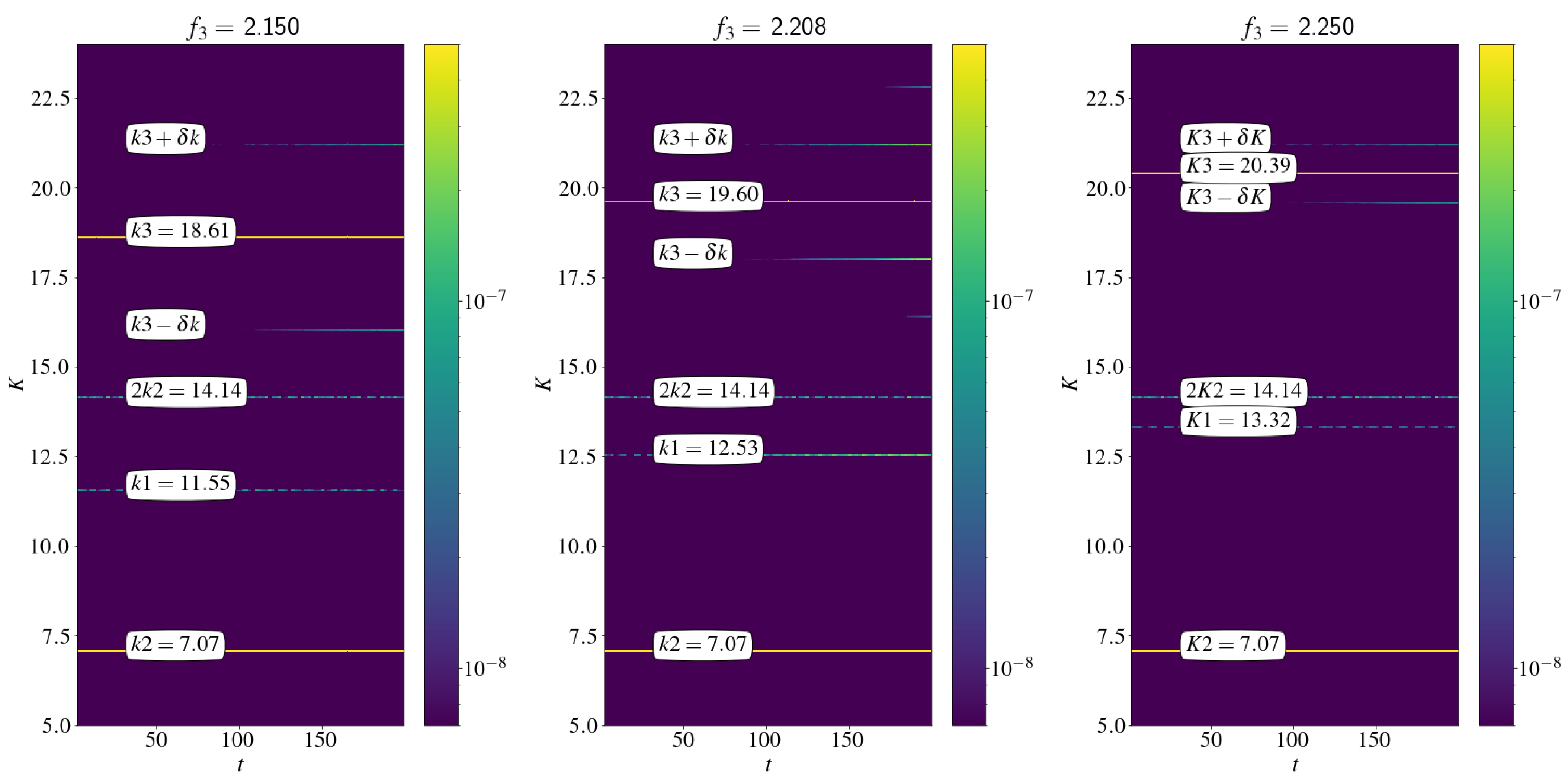
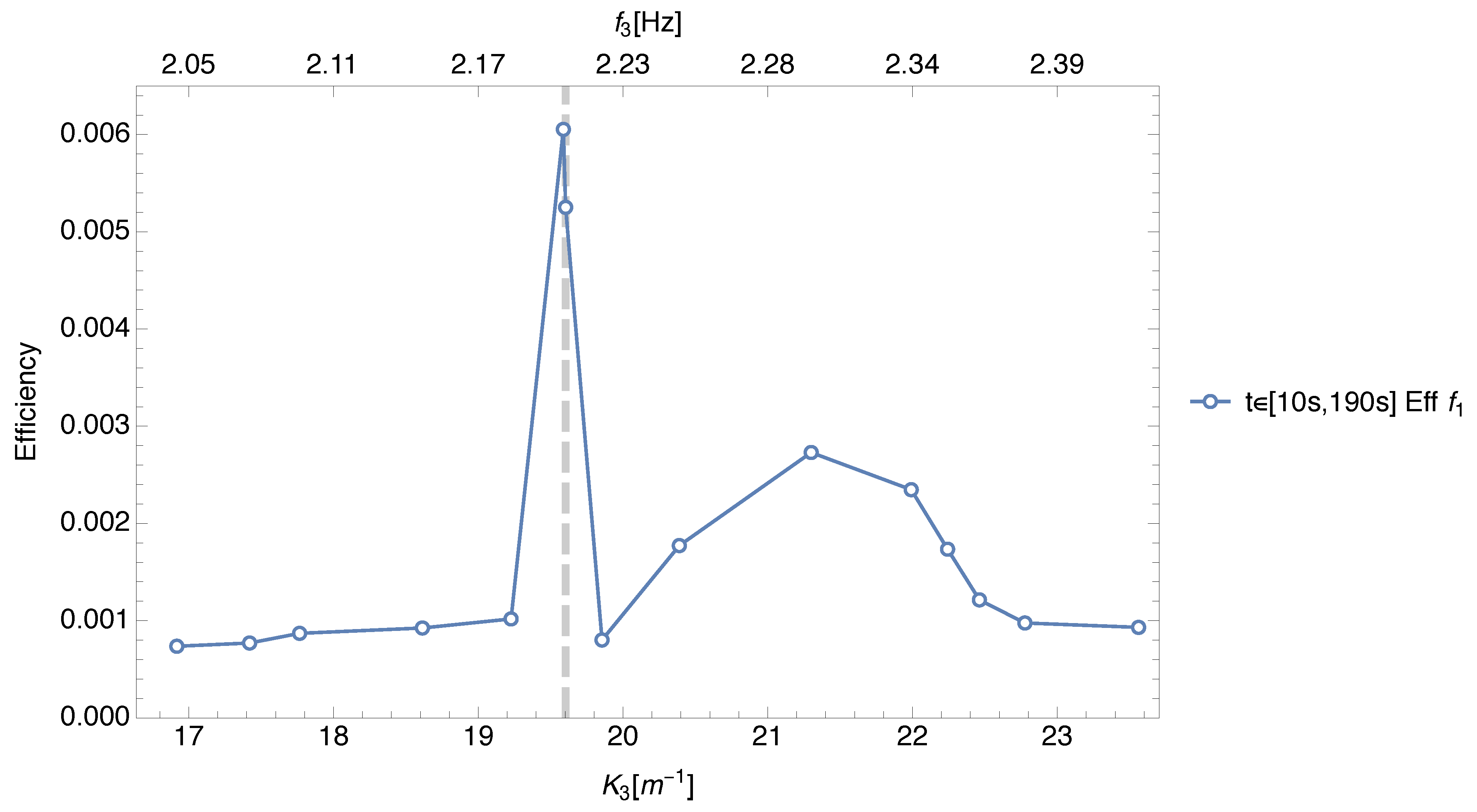
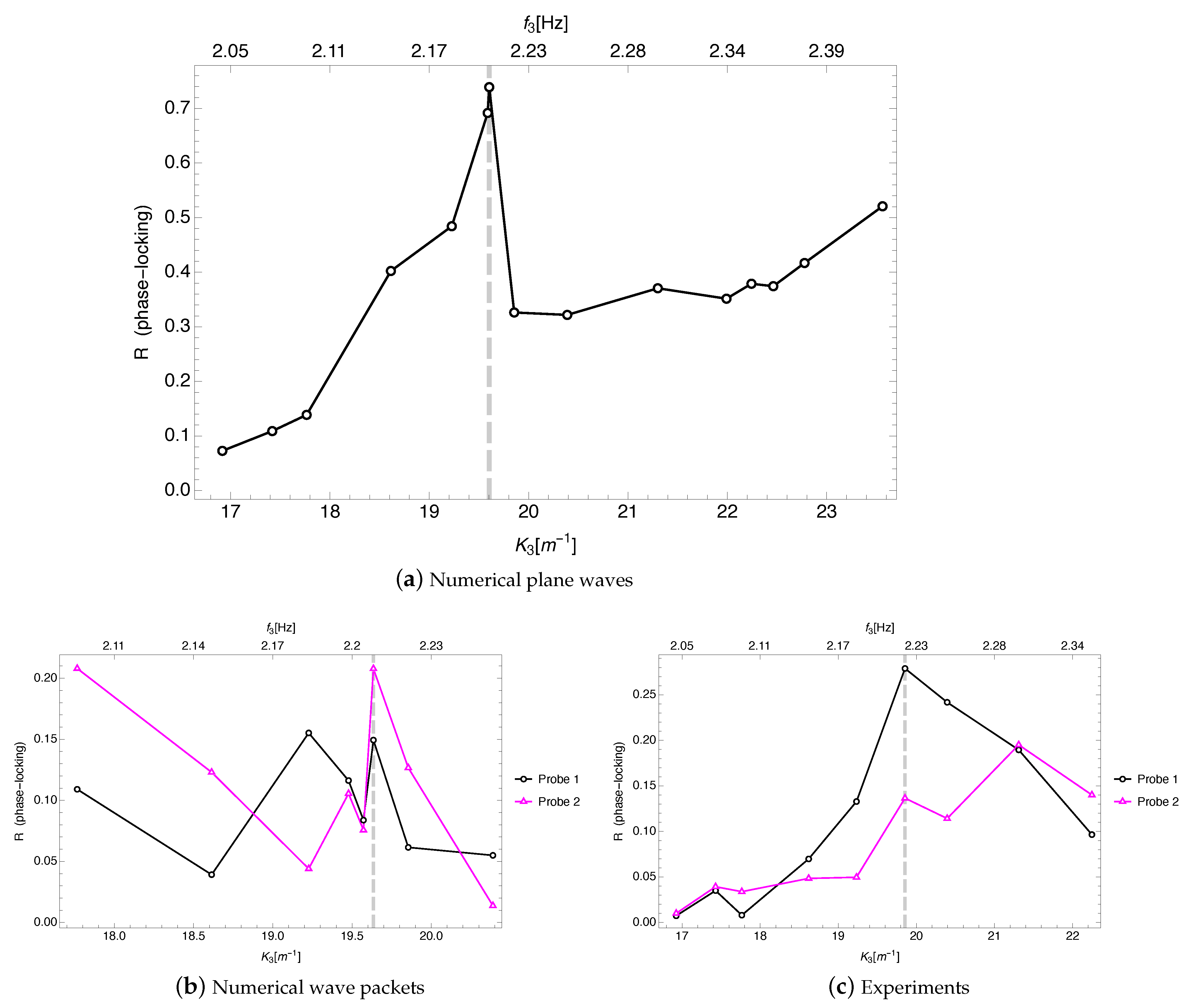
3.1. Encountering Plane Waves

In order to diagnose growth of energy in the target mode we define a measure of efficiency using the normal variables, themselves computed from the natural ones by inverting (14) and (15):
E k ( t ) = ω k a k a k * H ,
where H is the full Hamiltonian, defined in Equation (12). We show max t [ 0 , 500 ] E K 1 ( t ) against K 3 in Figure 2 for β = 1 and β = 0.75 . A distinct, but narrow peak is observed near the predicted resonant K 3 (marked with vertical line). The efficiencies are around 1.5 % at the peak for β = 1 , with the time series of E K ( t ) shown in Figure 3 demonstrating sustained growth in mode a K 1 over approximately 250 s in the resonant case, and no growth off resonance. Of note is the width of the resonant peak in K 3 ; coarser sampling of the initial wavenumber (or frequency) space will likely miss the optimal value for the resonance in the simulations. Due to nonlinear corrections the peak does not appear precisely at K 3 = 1250 2 π L but slightly displaced at K 3 = 1248 2 π L ; namely, a difference in wavelength of δ λ 0.5 mm or in frequency δ f 0.0018 Hz.
Figure 3 also shows the time series for the efficiency (or amplitude) of a K 3 . This shows a decrease of energy at late time which is generic across all of the calculations and only moderated slightly by the resonance. To determine which other nonlinear interactions are important in this system we examine the wavenumber spectrum as a function of time, plotted in Figure 4. Aside from K 1 , K 2 , K 3 we can observe 2 K 2 having energy from early time, and side-bands of K 3 namely K 3 ± δ K with δ K = 2 K 2 K 1 growing at late times due to modulational instability. This is the reason for the decrease observed in a K 3 . Importantly this is a background effect, present in all cases, and does not hinder the five-wave resonance under consideration.
To mimic the diagnostics available in a physical experiment we also seek evidence of resonant transfer in a time series of a numerical ‘probe’ measurement of the surface elevation, namely ζ ( x p , t ) , where x p = L / 2 + 2 m is the fixed location in the domain for the probe. The choice of x p is arbitrary in the plane wave case, however this choice is made to be in keeping with the experiments in Section 4. The resonance should be observed by an increase in the temporal linear frequency f 1 in this measure. In order to diagnose such growth we create a frequency-time figure using a wavelet transform in the form of a ‘scaleogram’. With a duration of t = 200 s, sampling 10,000 points in time and performing a wavelet transform using Gabor wavelets with 48 oscillations, with a scale resolution of 11 frequency scales along with 64 voices per scale, we obtain Figure 5. Three cases are shown (at the same K 3 as the time series of Figure 3) which demonstrates, for f 3 2.206 Hz, the growth in time of the signal with frequency f 1 , marked with a horizontal blue dashed line. A similar efficiency can be defined using this measure defined as the sum of the squares of the scaleogram signals in Figure 5, on a strip of width 0.05 f 1 about f 1 and between t [10,190], divided by the sum of squares over the whole range of frequencies, shown in Figure 6. From these data emerges a qualitatively similar result as for the spatial Fourier efficiency shown in Figure 2, with a distinct peak around K 3 = 1248 2 π L .
To finalise the plane-wave case we provide a piece of analysis that connects with the theoretical derivation of the Hamiltonian system in the resonant case. Recall that for the symmetric initial conditions we took, the resonant case is expected to be integrable. A useful integrability test is to plot variables that would normally behave independently, except when the system is near integrable. To this end we provide joint probability density functions over the simulation time t [0, 200 s] of the quintet phase ϕ + ( t ) = 2 ϕ 2 ( t ) + ϕ 2 ( t ) ϕ 3 ( t ) ϕ 1 ( t ) versus its time derivative d ϕ + d t ( t ) in Figure 7. The resonant case, f 1 = 2.206 Hz, shows a clear reduction of the system’s dimension, evidencing the onset of a coherent, near-integrable regime which we attribute to the resonance.
A careful investigation of the source of this coherence shows that it really arises due to the increase in amplitude felt by a K 1 at resonance. Off resonance the phase rotates with a greater deal of variability, since the complex amplitude is closer to the origin, than in the resonant case where a K 1 has larger absolute value and therefore rotates at a more consistent rate, given by the linear frequency ω K . Notice also that in the symmetrical “encountering waves” setup studied in our numerical simulations, the symmetry ϕ j = ϕ j is valid at all times. This leads to the identity ϕ + = ϕ 1 + ϕ 2 ϕ 3 , indicating that the 5-wave resonance is directly related to a phase locking between the three basic waves.

3.2. Encountering Wave Packets

In order to determine how reproducible the above result using plane waves may be in a physical experiment, we adapt the initial condition of the previous section into two types of spatially localised, propagating initial data. We wish to examine the joint effects of the dispersion of waves from a source (wavemaker), the limited interaction time and the limited spatial interaction region, due to the finiteness of the domain. The first such initial condition we consider is a localised wave packet at the centre of the domain containing the same wave content as in the planar case of the previous section, i.e.,
ζ ( x , 0 ) = ζ ^ K 2 e i K 2 x + ζ ^ K 3 e i K 3 x e 36 x x 0 σ 30 , Φ ( x , 0 ) = 0 ,
with x 0 = L / 2 and σ = L / 4 giving a packet occupying half of the domain, composed of both left propagating waves (i.e., propagating towards x direction) and right propagating waves (i.e., propagating towards + x direction). This situation is close to the plane-wave case: Setting progressively larger σ would interpolate towards plane waves. It is also analogous to starting measurements in an experiment once the waves have encountered and overlapped, but neglects any interactions which occur as they start to encounter. As the waves propagate away from the centre of the domain the region nonlinearly interacting shrinks until eventually the required waves are no longer coincident. This will be referred to as the ‘A’ configuration.
The ‘B’ configuration has similar half-domain localised wave packets, but now two of them, which contain either left or right propagating waves in such a way as to have encountering waves at the centre, i.e.,
ζ r ( x , 0 ) = K 2 4 g 1 / 4 a K 2 e i K 2 x + K 3 4 g 1 / 4 a K 3 e i K 3 x e 36 x L / 4 σ 30 ,
Φ r ( x , 0 ) = i g 4 K 2 1 / 4 a K 2 e i K 2 x + g 4 K 3 1 / 4 a K 3 e i K 3 x e 36 x L / 4 σ 30 ,
ζ l ( x , 0 ) = K 2 4 g 1 / 4 a K 2 * e i K 2 x + K 3 4 g 1 / 4 a K 3 * e i K 3 x e 36 x 3 L / 4 σ 30 ,
Φ l ( x , 0 ) = i g 4 K 2 1 / 4 a K 2 * e i K 2 x + g 4 K 3 1 / 4 a K 3 * e i K 3 x e 36 x 3 L / 4 σ 30 ,
where the subscripts r and l are the right and left propagating packets, respectively, and the centre of each packet is x 0 = L / 4 from the centre. The full initial condition is ζ = ζ r + ζ l and ϕ = ϕ r + ϕ l , see upper panel of Figure 8. This configuration will therefore capture more dispersion and temporal behaviour as the waves propagate across one another, but will have have a smaller overall region at any given time where the necessary waves are coincident. Between these two configurations we have convenient middle ground between the plane wave case and the full physical experiment, to help ascertain where differences are observed and perhaps show how to design better experiments in the future.
We perform the same parameterised sweep of f 3 as in Section 3.1 to intersect the resonance condition and seek increased transfer efficiency. max E K 1 is shown in Figure 2 along side the plane wave case and time series are shown in Figure 9. The efficiency is now much lower but a broader peak persists, case A showing a stronger signal than B. Now the time series demonstrates, in both cases but less pronounced in case A, that growth into K 1 is more transient and less sustained than in the plane case, the peak in | a K 1 | occurring within the first 10–20 s.
The reduction in overall efficiency and reduction in sustained growth is, of course, to be expected since the interaction is now localised in space and is not globally instantaneous across the domain as in the plane wave case. In addition, although the initial local surface elevations are comparable the overall energy content in the modes is reduced by the localising kernel used to create the individual packets. Finally it should be noted that the initial spectrum is broadened by the localisation, this means that first there is a wider range of K 3 experiencing resonant (or quasi-resonant) transfer, but also it is possible for more than just the single target K 1 to experience resonant growth. We may take this into account by allowing more modes to contribute to the efficiency definition about the central K 1 . However a better approach, having established that some resonant interactions do persist is to return to the wavelet, scaleogram, wave probe analysis as described above and see if we can observe transfers using a local measure of the surface height.
Given the moderately stronger signal in the efficiency E K using the A initial condition, we analyse the probe measurements from this case. We now use two probe locations x p = L / 2 ± 2 m first to correspond to the physical experiments in the proceeding section, but also noticing that a symmetry breaking occurs, with a more definite peak in the wavelet based efficiency in the left hand probe at L / 2 2 m as shown in the scaleograms in Figure 10 and the ‘sum of squares’ efficiency in Figure 11.
Figure 10 shows the same 3 cases as in Figure 9a and the initial frequency f 3 is in evidence. Naturally, due to the broadening of the spectrum and the shorter time window in which the waves will be encountering the probe, the scaleogram shows a far more scattered set of frequencies. As described the left hand probe shows a discernible brightness about the target f 1 line for f 3 = 2.204 Hz where the peak in E K 1 is also observed in Figure 2, however this is not easily seen in the right hand probe. This opens up some interesting questions about symmetry breaking and measurement for a physical experiment. The symmetry breaking presumably arises due to numerical error in preparing the localised initial condition and/or due to instability of the localised initial condition, including processes due to nonlinear interactions. There are other frequencies in these plots at which a coherent signal is observed; these are due to other nonlinear interactions, e.g., the side-band instability at K 3 ± δ K described earlier, which we will not elaborate upon here.
From these results we may conclude that quite long interaction times and regions will be required to make definitive observations of a five-wave resonance of this type.

4. Experiments

We performed preliminary experiments in a water wave tank to search for this resonance. The experimental setup, shown in Figure 12, consists of a linear wave tank (length = 35 m) with identical right-angle wedges (wavemakers) on each end that are oscillated vertically. The water mass at rest has a depth of 0.55 m. Two probes are located symmetrically at a distance of 15.5 m from the corresponding nearest end. The distance between the probes is 4 m.
See, in Appendix B, probe calibration curves and consistency tests.

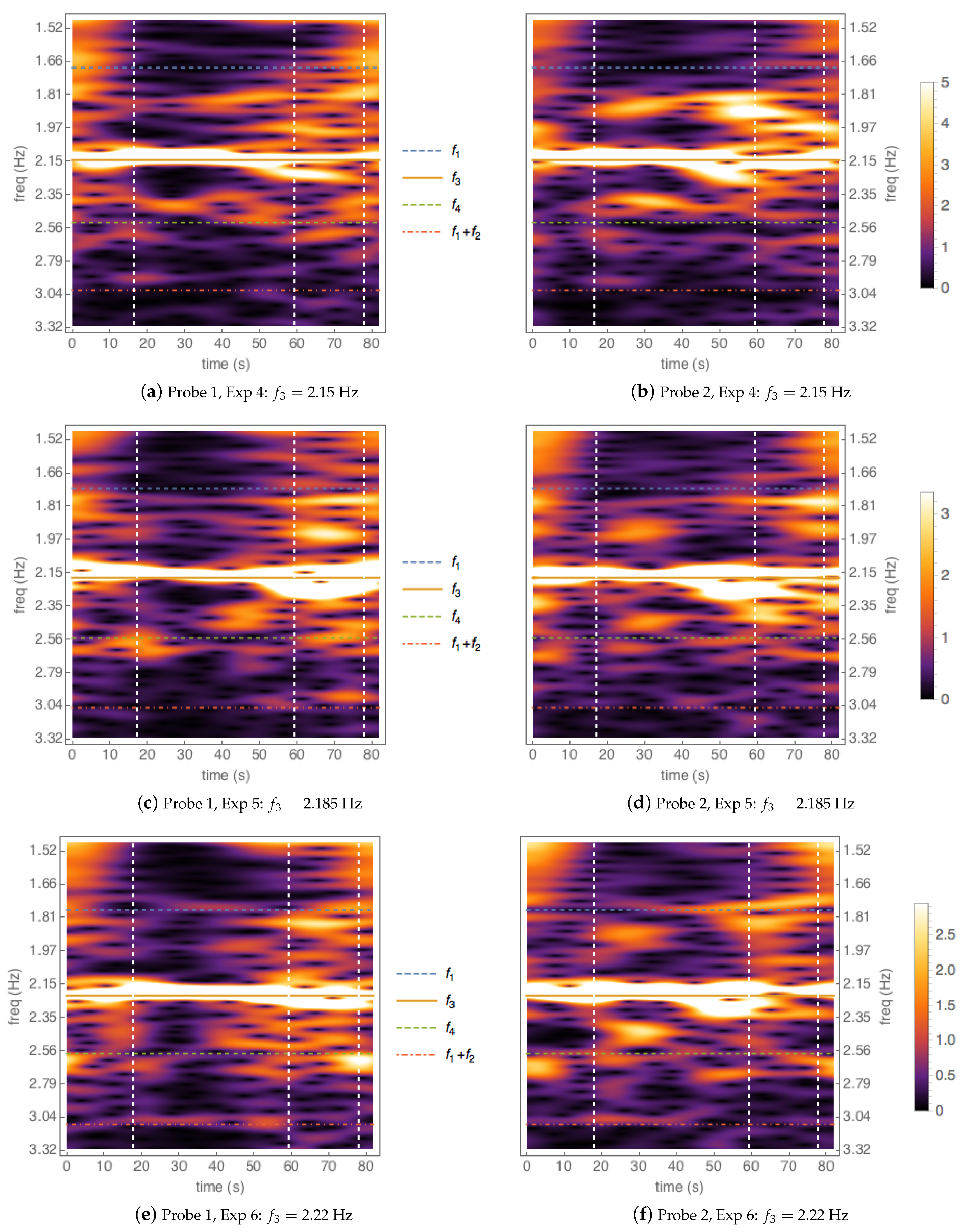
Encountering Wavepacket Experiments

In our experiments the water depth is finite and therefore one should use the gravity-wave dispersion relation 2 π f ( k ) = g k tanh ( k h ) , where g = 9.8 m s 1 is the acceleration of gravity and h = 0.55 m is the water depth. However, for the frequencies studied ( f 1.33 Hz) the relative error with respect to the infinite-depth approximation 2 π f ( k ) = g | k | is less than 10 5 so we can use this latter approximation. Equivalently, for the frequencies tested, deep water can be assumed. We perform 9 experiments. On each experiment, the two wavemakers operate with the same oscillation pattern:
η ( t ) = A 2 cos ( 2 π f 2 t ) + A 3 cos ( 2 π f 3 t ) ,
consisting of the sum of two monochromatic oscillations: The first one with a base fixed frequency f 2 = 1.33 Hz corresponding to wavevectors ± K 2 = ± 7.131 m 1 and with a fixed amplitude of approximately A 2 0.06 / K 2 (so steepness is A 2 K 2 = 0.06 ), while the second one has a changeable frequency f 3 , depending on the experiment, and a changeable amplitude A 3 0.12 / K 3 again so that the steepness is fixed at 0.12 . Table 1 summarises the range of values of wavemaker frequencies f 3 used in the 9 experiments, with the corresponding amplitudes A 3 used.
In each experiment, therefore, as a result of the wavemakers’ activity, two encountering wave trains with central wavevectors K 2 , K 3 , K 2 , K 3 will approach the probes, and will eventually encounter each other, triggering nonlinear interactions. If the theory is correct, when K 3 / K 2 = 25 / 9 the five-wave resonance should produce waves with wavevectors ± K 1 = ± 16 K 2 / 9 , as explained in Equation (16). The frequencies are proportional to the square roots of the wavenumbers, and as explained in the text right after Equation (16), at resonance we would have f 1 : f 2 : f 3 = 4 : 3 : 5 . Now, eventually these daughter waves would reach the probes, which would record a signal with frequency f 1 , reso = 4 f 2 / 3 . Theoretically, this five-wave resonance should occur near Experiment 6, because in that experiment we have K 3 = 4 π 2 g 1 f 3 2 = 19.85 m 1 and as K 2 = 7.131 m 1 , we would get K 3 / K 2 2.78 which is very close to 25 / 9 . Similarly, the corresponding frequency of the oscillations produced by the nonlinear resonant interactions, f 1 = g K 1 / 2 π = g ( K 3 K 2 ) / 2 π 1.78 Hz, would be very close to f 1 , reso = 4 f 2 / 3 1.77 Hz.
Probe measurements are started when the wavepackets reach the probes. For each experiment we perform measurements on each probe, at intervals of Δ t = 0.02 s and during a time of 81.9 s, corresponding to a total of N = 4096 data points per probe per experiment. Figure 13 shows the time series for experiment 7, which is the one that shows a stronger signal for the target frequency f 1 , as we will see when we analyse the scalograms. From the time series we can see that the two probes’ measured oscillations are quite close and in phase: The dominant frequency in the plot is f 2 = 1.33 Hz corresponding to the wavevectors ± K 2 . Modulations about this main frequency correspond to a combination of frequencies f 3 and f 1 along with a spectrum of less important frequencies, including harmonics. The fact that the two probes’ signals are not exactly the same is reminiscent of the symmetry breaking observed in the numerical case, and may be due to slight differences in the experimental conditions and the subsequent nonlinear amplification of these differences.
As the fastest waves are the ones with wavevectors ± K 2 (at the fixed frequency f 2 = 1.33 Hz in the experiment), one can assume these waves will reach the probes first. We recall that, in the experiments, the initial measurement time t = 0 corresponds precisely to the time when the waves reach the probes for the first time. As the group velocity of the waves with wavevectors ± K 3 is less than the group velocity of the waves with wavevectors ± K 2 , we expect to see no effect from the nonlinear interactions (and in particular no generation of ± K 1 wavevectors) in the early stages. To be more precise, a simple analysis of the five-wave resonance Equation (16) shows that nonlinearly-produced wavevectors ± K 1 could be measured by the probes from the moment the wavevectors ± K 3 reach the probes. This time can be calculated explicitly for each experiment, giving, for experiments 1 to 9, t 0 = { 14.44 , 15.04 , 15.44 , 16.44 , 17.14 , 17.84 , 18.42 , 19.42 , 20.42 } s. The leftmost vertical marker line in Figure 13 corresponds to this “first measurement” time.
It is also evident from Figure 13 that wave amplitudes become larger near t 60 s. This is due to the reflected wavepackets with wavevectors ± K 2 , which after reflection from the walls of the tank arrive back at the probes. After this time we expect a stronger signal for the nonlinearly-produced wavevectors ± K 1 in the probes. The time this happens is t 1 = 59.38 s, independent from the experiment. The rightmost vertical marker line in Figure 13 corresponds to this “second measurement” time.
In order to understand the frequency content of these signals, we apply a wavelet transform on them. Wavelet scaleograms show the time evolution of the energy content over a range of frequencies. By trial and error we found that a good compromise is struck between frequency resolution and time resolution in the wavelet transform by choosing a Gabor wavelet with 96 oscillations and with the usual scale resolution of log 2 ( 4096 / 2 ) = 11 and a total of 256 voices per scale. Before analysing the real data, Figure 14 shows density-plot scaleograms corresponding to artificial signals containing only four frequencies:
σ artif ( t ) = 10 sin ( 2 π f 2 t ) + 3 sin ( 2 π f 3 t ) + 0.3 sin ( 2 π f 1 t ) + 0.3 sin ( 2 π f 4 t ) ,
where f 3 is chosen from the list in Table 1 and f 1 , f 4 are two possible target frequencies defined in terms of the dispersion relation by 2 π f 1 = g K 1 and 2 π f 4 = g K 4 , where K 1 = K 3 K 2 and K 4 = K 3 + K 2 are target wavevectors that could be generated by nonlinear interactions in the experiments (notice that 2 π f 3 = g K 3 defines the wavevector K 3 ). Apart from f 2 = 1.33 Hz which is fixed, these frequencies depend on the experiment (but are completely determined by it) according to Table 1. The scaleograms show spurious boundary effects at early and late times for the frequency f 3 . For the frequencies f 1 and f 4 the boundary effects are minimal. The plots show that these two frequencies are resolved within a band of width Δ f = 0.09 f . Thus, a real signal from the experiments at a given frequency will be expected to have a comparable width. This will be useful when estimating the relative energy in a frequency.
In Figure 15, Figure 16 and Figure 17 we show the scaleograms obtained from probe 1 data (left panels) and probe 2 data (right panels). For each panel, vertical lines analogous to those in Figure 13 indicate the theoretical first time t 0 when nonlinearly produced target frequency f 1 due to the five-wave resonance can be measured by the probes (leftmost line), the theoretical time t 1 when the wavepackets arrive back at the probes after reflecting from the tank walls (middle line), and the time beyond which the scaleograms show spurious boundary effects, as evidenced in Figure 14 (rightmost line). The figures also show horizontal lines corresponding to the theoretical frequencies f 1 , f 3 , f 4 derived from the wavevectors ± K 1 , ± K 3 , ± K 4 , and a theoretical harmonic f 1 + f 2 . It is apparent that experiment 6 shows some activity in the f 1 line, as well as the line f 1 + f 2 . However, the next experiment (number 7) shows a more convincing signal at f 1 , apparently resolved, particularly at the late stages after t = t 1 = 59.38 s.
In order to provide a more quantitative measure of the signals shown by the scaleograms, we calculate the relative energy of the wavelet transforms that are plotted in the scaleograms, for the frequency f 1 . We do this by defining an early-time energy by the sum of squares between t = t 0 and t = t 1 = 59.38 s, and on a strip of width Δ f = 0.09 f 1 about f 1 . We then divide this energy by the total energy over the time interval [ t 0 , 59.38 s] and over the whole frequency range (including f 2 which is not shown). The result is an “early-time efficiency” which we plot in Figure 18, dashed lines, for each probe. Similarly, we define a late-time energy by the sum of squares between t = t 1 = 59.38 s and t = 77.92 s, and on a strip of width Δ f = 0.09 f 1 about f 1 . We then divide this energy by the total energy over the time interval [59.38 s, 77.92 s] and over the whole frequency range (including f 2 , not shown). The result is a “late-time efficiency” which we plot in Figure 18, solid lines, for each probe. It is evident from these plots that there is an efficiency peak that stands out, and although it is modest ( 0.5 % efficiency) it nevertheless shows that considering the short times involved there is scope for a measurement of the theoretical five-wave resonance, perhaps in a larger tank and with larger amplitudes so that the effect can be clearly obtained.

5. Conclusions and Discussion

In this work we proposed to study the minimal resonant configuration of water gravity waves in one-dimensional propagation. The resulting 5-wave resonances are based on a triad of wavevectors along with their negatives, leading to a scenario of encountering wavepackets, which has an experimental appeal. The problem poses interesting challenges in all fronts:
  • On the theoretical front, the 5-wave resonant manifold and the interaction coefficients on this resonant manifold had been obtained in a series of papers over two decades ago [4,5,6], triggered by the discovery that the interaction coefficients vanish identically on the 4-wave resonant manifold for one-dimensional propagation of water gravity waves [3]. We used these results to find the simplest 5-wave resonance that can be made out of a triad of wavevectors and their negatives, and calculated its normal-form Hamiltonian. We proved that the system is not integrable, but it lacks just one constant of motion to become integrable, so symmetric scenarios can produce integrable systems.
  • On the front of numerical simulations of the governing partial differential equations, the equations had been obtained over five decades ago [15], as a power series in terms of the steepness effectively. The numerical implementation we needed to use in order to accurately resolve 5-wave interactions is the one that uses up to 6-wave interactions in a pseudo-spectral setting [40]. Such an implementation requires a higher-than-usual dealiasing and thus can get quite expensive in terms of the required spectral resolution. We managed to validate our implementation against some benchmarks, and were able to establish the existence of the resonance and quantify its effects in terms of the energy transferred to target modes. We considered encountering plane waves and also encountering wave packets, in a simulated tank that is 300 m long. The plane-wave case provided the most efficient energy transfer in terms of Hamiltonian energy, while the wavepackets case provided a higher efficiency in terms of the probe measurements of surface elevation at a point along the tank.
  • On the experimental front the main difficulty is to fine tune the amplitudes and frequencies in order to capture the resonance, but we got this from hindsight. Our preliminary experiments seem to show that the resonance exists physically, although as can be seen in Figure 18, the efficiency is relatively small.
We learned from our more recent numerical experiments that the resonance peak has a narrow width. For this reason we propose to conduct experiments in much longer wave flumes with much larger amplitudes of lower frequency waves. In addition, the study of the second resonant quintet (17) obtained theoretically, and/or the exploration of optimal initial conditions, may make it easier to find a resonance in experiments as well as numerical simulations. In future work we plan to extend this type of minimal search to gravity-capillary waves and to gravity waves in two-dimensional propagation.
We would like to end on a positive note, by reporting on the following phase-locking analysis between the three scenarios studied: Numerical encountering plane waves, numerical encountering wave packets, and experimental encountering waves. We will establish that the triad phases get locked near our theoretical resonance, thus providing an independent piece of evidence that the resonance is indeed taking place. We explain briefly how this is done. Using the probe data for each scenario and each “experiment” within a given scenario, we perform pass-band filters around each of the three important frequencies f 1 , f 2 , f 3 , with width 0.09 f . Each one of these three filtered signals is then extended via the analytic signal approach using a Hilbert transform (see, for example, [46]) in order to get the “conjugate” signal and thus calculate the “analytic phases” denoted by the time series φ 1 ( t ) , φ 2 ( t ) , φ 3 ( t ) . These phases contain the fast time dependence 2 π f j t , respectively. After subtracting this fast time dependence, obtain the new phases φ ˜ j ( t ) = φ 1 ( t ) 2 π f j t , j = 1 , 2 , 3 . We then calculate the triad phase
φ ( t ) : = φ ˜ 1 ( t ) + φ ˜ 2 ( t ) φ ˜ 3 ( t ) .
The phase-locking value for this signal is defined by (see, e.g., [47]):
R : = | exp ( i φ ( t ) ) t | [ 0 , 1 ] ,
where · t denotes time average over the whole time series, and | · | denotes modulus. A phase-locking value close to 1 denotes a situation where the corresponding phase is locked at a given value for most of the time. The resulting phase-locking values, for the different scenarios and the different experiments, are plotted in Figure 19, using similar notation as in the efficiency Figure 6, Figure 11 and Figure 18. It is evident that in each scenario the phase-locking value is maximum precisely at the resonant case (denoted in each panel with a vertical dashed line), thus confirming that the 5-wave resonance not only provides larger target amplitudes but also strong phase synchronisations amongst the interacting modes. Notice that the effect of symmetry breaking is again patent in the numerical wave packets case, cf. Figure 19b, as well as in the experimental case, cf. Figure 19c. In each case, one of the probes shows a clear global maximum of phase-locking R at the resonance, while the other probe has a local maximum at the resonance and a global maximum at another place. This behaviour is consistent with the efficiency plots in Figure 11 and Figure 18: The probes that show a higher efficiency peak in these figures, correspond precisely to the probes that show a clear and strong maximum of the phase-locking value R in Figure 19b,c.

Author Contributions

Conceptualization, D.L., M.P. and M.D.B.; theoretical investigation and modelling, D.L., S.W., R.I. and M.D.B.; numerical simulations and analysis, D.L. and M.D.B.; experimental investigation, M.P., D.-Y.L.; writing—original draft preparation, review and editing, D.L., M.P., R.I. and M.D.B. All authors have read and agreed to the published version of the manuscript.

Funding

R.I. is partially supported by the Bulgarian National Science Fund, grant KΠ -06H42/2 from 27.11.2020.

Data Availability Statement

The data presented in this study are available on request from the corresponding author ([email protected]).

Acknowledgments

We thank Wooyoung Choi for providing us with key references about the fifth-order code.

Conflicts of Interest

The authors declare no conflict of interest. The funders had no role in the design of the study; in the collection, analyses, or interpretation of data; in the writing of the manuscript, or in the decision to publish the results.

Appendix A. Construction of 5-Wave Resonances Using Only Three Different Positive Wavevectors J1, J2, J3 (with 0 < J2 < J1 and J3 = J1 + J2) Along with Their Negatives

Consider three different positive wavevectors J 1 , J 2 , J 3 , with 0 < J 2 < J 1 and J 3 = J 1 + J 2 , along with their negatives J 1 , J 2 J 3 . These are six wavevectors in total. Using these six wavevectors only, we want to solve the equations determining 5-wave resonances for deep water waves with dispersion relation ω ( k ) = g | k | . As obtained in [5], and using the notation in that reference, the problem is reduced to solving the momentum equation and the frequency condition, respectively:
k 1 + k 2 + k 3 = p + q , | k 1 | + | k 2 | + | k 3 | = | p | + | q | ,
for the wavevectors k 1 , k 2 , k 3 , p , q Z . The solution given in the reference establishes five cases:
(i)
All wavevectors are positive.
(ii)
p , q > 0 , and one of the k 1 , k 2 , k 3 is negative.
(iii)
p , q > 0 , and two of the k 1 , k 2 , k 3 are negative.
(iv)
p , q have different signs, and k 1 , k 2 , k 3 > 0 .
(v)
p , q have different signs, and one of the k 1 , k 2 , k 3 is negative.
Recall that we need to use the six wavevectors mentioned at the beginning, namely we have k 1 , k 2 , k 3 , p , q { ± J 1 , ± J 2 , ± J 3 } . Moreover, a wavevector cannot appear in both sides of the momentum equation, as that would lead to a triad resonance, which is known not to exist. Therefore one must impose in what follows the condition
{ k 1 , k 2 , k 3 } { p , q } = .
Notice however that, on a given side of the momentum equation, it is possible to repeat wavevectors. Namely, it is possible to have # { k 1 , k 2 , k 3 } < 3 and/or # { p , q } < 2 . We now consider one by one the five possible cases including all relevant subcases. It turns out that only subcases (v.1.c) and (v.2.b) below have solutions: the resonances (16) and (17) presented in this paper.
(i)
As all wavevectors are positive, we need to restrict k 1 , k 2 , k 3 , p , q { J 1 , J 2 , J 3 } . As we must impose (A1) we conclude { k 1 , k 2 , k 3 } { J 1 , J 2 , J 3 } . Therefore we have two subcases: (i.1) k 1 = k 2 = k 3 and (i.2) k 1 = k 2 k 3 . In subcase (i.1) the option p = q k 1 leads to the momentum equation 3 k 1 = 2 p but the resonance condition is 3 k 1 = 2 p which contradicts the momentum equation. The only other option is p q k 1 p . We have the following three instances:
(i.1.a) k 1 = k 2 = k 3 = J 2 , p = J 1 , q = J 3 . Here, the momentum equation is 3 J 2 = J 1 + J 3 which implies J 2 = J 1 and thus J 3 = 2 J 2 , so the resonance condition is 3 J 2 = J 2 + 2 J 2 , which has no solution.
(i.1.b) k 1 = k 2 = k 3 = J 1 p = J 2 , q = J 3 . Here, the momentum equation is 3 J 1 = J 2 + J 3 which implies J 1 = J 2 and thus J 3 = 2 J 2 , so the resonance condition is 3 J 2 = J 2 + 2 J 2 , which has no solution.
(i.1.c) k 1 = k 2 = k 3 = J 3 p = J 1 , q = J 2 . Here, the momentum equation is 3 J 3 = J 1 + J 2 which implies J 3 = 0 , with no solution.
In conclusion subcase (i.1) has no solution. We now study subcase (i.2) k 1 = k 2 k 3 . In this subcase we must have p = q k j for all j = 1 , 2 , 3 . We have the following six instances:
(i.2.a) k 1 = k 2 = J 2 , k 3 = J 1 , p = q = J 3 . Here, the momentum equation is 2 J 2 + J 1 = 2 J 3 which implies J 1 = 2 J 1 , with no solution.
(i.2.b) k 1 = k 2 = J 1 , k 3 = J 2 , p = q = J 3 . Here, the momentum equation is 2 J 1 + J 2 = 2 J 3 which implies J 2 = 2 J 2 , with no solution.
(i.2.c) k 1 = k 2 = J 2 , k 3 = J 3 , p = q = J 1 . Here, the momentum equation is 2 J 2 + J 3 = 2 J 1 which implies J 1 = 3 J 2 and thus J 3 = 4 J 2 , so the resonance condition is 2 J 2 + 4 J 2 = 2 3 J 2 , which has no solution.
(i.2.d) k 1 = k 2 = J 1 , k 3 = J 3 , p = q = J 2 . Here, the momentum equation is 2 J 1 + J 3 = 2 J 2 which implies J 2 = 3 J 1 which has no solution (because J 2 J 1 ).
(i.2.e) k 1 = k 2 = J 3 , k 3 = J 2 , p = q = J 1 . Here, the momentum equation is 2 J 3 + J 2 = 2 J 1 which implies 3 J 2 = 0 , with no solution.
(i.2.f) k 1 = k 2 = J 3 , k 3 = J 1 , p = q = J 2 . Here, the momentum equation is 2 J 3 + J 1 = 2 J 2 which implies 3 J 1 = 0 , with no solution.
In conclusion subcase (i.2) has no solution. Therefore, case (i) has no solution.
(ii)
In this case we restrict k 1 , k 2 , p , q { J 1 , J 2 , J 3 } and k 3 { J 1 , J 2 , J 3 } , with { k 1 , k 2 } { p , q } = following from (A1). The momentum condition reads k 1 + k 2 = | k 3 | + p + q . As in case (i) we have two subcases: (ii.1) k 1 = k 2 and (ii.2) k 1 k 2 . In subcase (ii.1) the option p = q k 1 leads to the momentum condition 2 k 1 = | k 3 | + 2 p , leading to | k 3 | = 2 ( k 1 p ) , so k 1 > p . However, the resonance condition reads 2 k 1 + | k 3 | = 2 p , leading to | k 3 | = 2 ( p k 1 ) , so p > k 1 , a contradiction.
The only other option is p q k 1 p . We have the following three instances:
(ii.1.a) k 1 = k 2 = J 2 , p = J 1 , q = J 3 . Here, the momentum condition is 2 J 2 = | k 3 | + J 1 + J 3 which implies J 2 = | k 3 | + 2 J 1 , with no solution (because J 2 J 1 ).
(ii.1.b) k 1 = k 2 = J 1 , p = J 2 , q = J 3 . Here, the momentum condition is 2 J 1 = | k 3 | + J 2 + J 3 which implies | k 3 | = J 1 2 J 2 , with only solution | k 3 | = J 2 , leading to J 1 = 3 J 2 and thus J 3 = 4 J 2 . Thus, the resonance condition reads 2 3 J 2 + J 2 = J 2 + 4 J 2 , with no solution.
(ii.1.c) k 1 = k 2 = J 3 , p = J 2 , q = J 1 . Here, the momentum condition is 2 J 3 = | k 3 | + J 2 + J 1 which implies | k 3 | = J 3 . The resonance condition reads 2 J 3 + J 3 = J 1 + J 2 , or 3 J 1 + J 2 = J 1 + J 2 . Squaring this gives 9 ( J 1 + J 2 ) = J 1 + J 2 + 2 J 1 J 2 , thus J 1 + J 2 = J 1 J 2 / 4 . Squaring again gives J 1 2 + J 2 2 + 2 J 1 J 2 = J 1 J 2 / 16 , with no real solution.
In conclusion subcase (ii.1) has no solution. We now study subcase (ii.2) k 1 k 2 . In this subcase we must have p = q k j for all j = 1 , 2 , 3 . We have the following three instances:
(ii.2.a) k 1 = J 2 , k 2 = J 1 , p = q = J 3 . Here, the momentum equation is J 2 + J 1 = | k 3 | + 2 J 3 , which implies 0 = | k 3 | + J 3 , with no solution.
(ii.2.b) k 1 = J 2 , k 2 = J 3 , p = q = J 1 . Here, the momentum equation is J 2 + J 3 = | k 3 | + 2 J 1 , which implies | k 3 | = 2 J 2 J 1 , so J 1 < 2 J 2 . As | k 3 | { J 1 , J 2 , J 3 } , we can check that | k 3 | = J 3 is not possible as it implies J 2 = 2 J 1 < 4 J 2 , a contradiction. We can check that the two remaining choices | k 3 | = J 1 or | k 3 | = J 2 imply J 1 = J 2 . So we conclude | k 3 | = J 1 = J 2 and thus J 3 = 2 J 2 . Thus, the resonance condition reads J 2 + 2 J 2 + J 2 = 2 J 2 , with no solution.
(ii.2.c) k 1 = J 1 , k 2 = J 3 , p = q = J 2 . Here, the momentum equation is J 1 + J 3 = | k 3 | + 2 J 2 , which implies | k 3 | = 2 J 1 J 2 . As | k 3 | { J 1 , J 2 , J 3 } , we can check that | k 3 | = J 3 implies J 1 = 2 J 2 and | k 3 | = J 3 = 3 J 2 , so the resonance condition reads 2 J 2 + 3 J 2 + 3 J 2 = 2 J 2 , with no solution. The two remaining choices | k 3 | = J 2 or | k 3 | = J 1 imply | k 3 | = J 1 = J 2 and J 3 = 2 J 2 . Thus, the resonance condition reads J 2 + 2 J 2 + J 2 = 2 J 2 , with no solution.
In conclusion subcase (ii.2) has no solution. Therefore, case (ii) has no solution.
(iii)
This case has zero interaction coefficients so it will not be considered.
(iv)
This case has zero interaction coefficients so it will not be considered.
(v)
In this case we restrict k 1 , k 2 , p { J 1 , J 2 , J 3 } and k 3 , q { J 1 , J 2 , J 3 } , with { k 1 , k 2 } { p } = and k 3 q following from (A1). Instead of considering explicitly all 27 possible instances we will use the results from [5] regarding inequalities amongst frequencies. These translate directly to inequalities amongst wavevectors, which in our notation can be summarised as:
k 1 k 2 < p , | k 3 | < | q | , p | q | .
As we assume without loss of generality J 2 J 1 < J 3 , it follows that p J 2 and | q | J 2 because J 2 is the smallest wavenumber. Thus, there are two subcases: (v.1) p = J 3 , q = J 1 , and (v.2) p = J 1 , q = J 3 .
In subcase (v.1) p = J 3 , q = J 1 , inequalities (A2) imply k 1 , k 2 < J 3 and k 3 = J 2 , with the now strict inequality J 2 < J 1 . There are three options:
(v.1.a) k 1 = k 2 = J 1 . Here the momentum condition reads 2 J 1 + ( J 2 ) = J 3 + ( J 1 ) , which simplifies to J 1 = J 2 , a contradiction.
(v.1.b) k 1 = J 2 , k 2 = J 1 . Here the momentum condition reads J 2 + J 1 + ( J 2 ) = J 3 + ( J 1 ) , which simplifies to J 1 = J 2 , a contradiction.
(v.1.c) k 1 = k 2 = J 2 . Here the momentum condition reads 2 J 2 + ( J 2 ) = J 3 + ( J 1 ) , which is identically satisfied (because J 3 = J 2 + J 1 ). We turn to the resonance condition to find 2 J 2 + J 2 = J 1 + J 2 + J 1 , or J 1 + J 2 = 3 J 2 J 1 . Squaring this gives J 1 + J 2 = 9 J 2 + J 1 6 J 1 J 2 , or 3 J 1 J 2 = 4 J 2 . Squaring again gives 9 J 1 = 16 J 2 . Thus J 1 = 16 J 2 / 9 and J 3 = 25 J 2 / 9 . In summary this leads to a 5-wave resonance parameterised by K Z + as follows:
9 K + 9 K + ( 9 K ) = 25 K + ( 16 K ) , 9 K + 9 K + 9 K = 25 K + 16 K .
In subcase (v.2) p = J 1 , q = J 3 , inequalities (A2) imply k 1 = k 2 = J 2 with the now strict inequality J 2 < J 1 , while | k 3 | < J 3 . There are thus two options:
(v.2.a) k 3 = J 2 . Here the momentum condition reads 2 J 2 + ( J 2 ) = J 1 + ( J 3 ) , which simplifies to J 2 = J 2 , a contradiction.
(v.2.b) k 3 = J 1 . Here the momentum condition reads 2 J 2 + ( J 1 ) = J 1 + ( J 3 ) , which simplifies to J 1 = 3 J 2 , thus J 3 = 4 J 2 . We turn to the resonance condition to find 2 J 2 + 3 J 2 = 3 J 2 + 4 J 2 , which is satisfied. In summary this leads to a 5-wave resonance parameterised by K Z + as follows:
K + K + ( 3 K ) = 3 K + ( 4 K ) , K + K + 3 K = 3 K + 4 K .

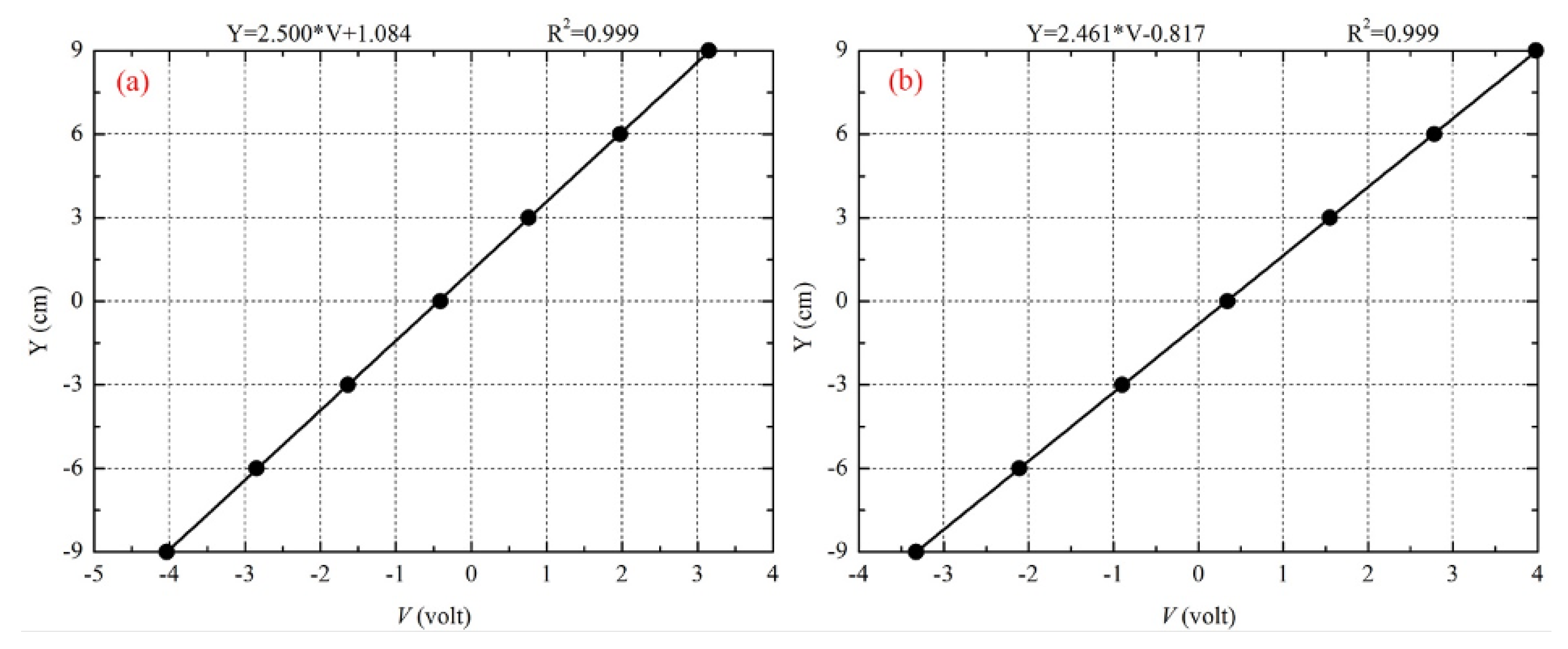
Appendix B. Probe Calibration and Wavemaker Tests

Figure A1 shows a picture of the probes arrangement in the experimental tank.
Figure A1. Picture of the experimental tank with a close up on the installed probes. The wire of each capacitance probe is directly facing each wedge.
Fluids 06 00205 g0a1
Figure A2 shows the results of the calibration of the probes. A linear regression gives R 2 = 0.999 for the relation between surface elevation and voltage, over a wide range of surface elevations (between 9 and 9 centimetres).
Figure A2. Calibration of the probes. (a) Probe 1. (b) Probe 2.
Fluids 06 00205 g0a2
Figure A3 shows the results of several cases of monochromatic wavemaker oscillations over a range of frequencies to be used in the interacting experiment. On each panel, solid black lines show the wave surfaces measured by probe 1 when the north wedge oscillates monochromatically, while red dashed lines correspond to probe 2 measurements when the south wedge is oscillated. Apart from slight differences between the two probes in panels (c) and (d) ( f = 2.22 Hz and f = 2.3 Hz, respectively), the waves are stable for the range of frequencies studied. It was found (figure not shown) that for frequencies above f = 2.35 Hz it was difficult to get regular wave trains, so we do not consider wavemaker frequencies higher than f = 2.35 Hz.
Figure A3. Tests of monochromatic wave generation by each wavemaker with the corresponding measurements by the closest probes. In each panel, the solid black line (red dashed line) represents the measurement by probe 1 (probe 2) of a wave generated by a monochromatic oscillation of the north wedge (south wedge). (a) Monochromatic frequency f = 1.33 Hz. (b) Monochromatic frequency f = 2.08 Hz. (c) Monochromatic frequency f = 2.22 Hz. (d) Monochromatic frequency f = 2.30 Hz.
Fluids 06 00205 g0a3

References

  1. Hammack, J.L.; Henderson, D.M. Resonant Interactions Among Surface-Water Waves. Annu. Rev. Fluid Mech. 1993, 25, 55–97. [Google Scholar]
  2. Nazarenko, S.; Lukaschuk, S. Wave Turbulence on Water Surface. Annu. Rev. Condens. Matter Phys. 2016, 7, 61–88. [Google Scholar]
  3. Dyachenko, A.; Zakharov, V.E. Is free-surface hydrodynamics an integrable system? Phys. Lett. A 1994, 190, 144–148. [Google Scholar] [CrossRef]
  4. Dyachenko, A.; Lvov, Y.; Zakharov, V.E. Five-wave interaction on the surface of deep fluid. Physica D 1995, 87, 233–261. [Google Scholar] [CrossRef]
  5. Lvov, Y. Effective five-wave Hamiltonian for surface water waves. Phys. Lett. A 1997, 230, 38–44. [Google Scholar] [CrossRef]
  6. Krasitskii, V.P. On reduced equations in the Hamiltonian theory of weakly nonlinear surface waves. J. Fluid Mech. 1994, 272, 1–20. [Google Scholar]
  7. Caponi, E.A.; Yuen, H.C.; Saffman, P.G. Instability and confined chaos in a nonlinear dispersive wave system. Phys. Fluids 1982, 25, 2159–2166. [Google Scholar] [CrossRef] [Green Version]
  8. Holmes, P. Chaotic motions in a weakly nonlinear model for surface waves. J. Fluid Mech. 1986, 162, 365–388. [Google Scholar]
  9. Trillo, S.; Wabnitz, S. Modulational Polarization Instabilities and Disorder in Birefringent Optical Fibers. In Nonlinearity with Disorder; Springer: Berlin/Heidelberg, Germany, 1992; pp. 269–281. [Google Scholar]
  10. Kim, W.; West, B.J. Chaotic properties of internal wave triad interactions. Phys. Fluids (1994-Present) 1997, 9, 632–647. [Google Scholar] [CrossRef]
  11. Hasselmann, K. On the non-linear energy transfer in a gravity-wave spectrum Part 1. General theory. J. Fluid Mech. 1962, 12, 481–500. [Google Scholar] [CrossRef]
  12. Hasselmann, K. On the non-linear energy transfer in a gravity wave spectrum Part 2. Conservation theorems; wave-particle analogy; irrevesibility. J. Fluid Mech. 1963, 15, 273–281. [Google Scholar] [CrossRef]
  13. Hasselmann, K. On the non-linear energy transfer in a gravity-wave spectrum. Part 3. Evaluation of the energy flux and swell-sea interaction for a Neumann spectrum. J. Fluid Mech. 1963, 15, 385–398. [Google Scholar] [CrossRef]
  14. Zakharov, V.E.; Filonenko, N.N. Weak turbulence of capillary waves. J. Appl. Mech. Tech. Phys. 1967, 8, 37–40. [Google Scholar] [CrossRef]
  15. Zakharov, V.E. Stability of periodic waves of finite amplitude on the surface of a deep fluid. J. Appl. Mech. Tech. Phys. 1968, 9, 190–194. [Google Scholar] [CrossRef]
  16. Newell, A.C.; Rumpf, B. Wave turbulence. Annu. Rev. Fluid Mech. 2011, 43, 59–78. [Google Scholar] [CrossRef] [Green Version]
  17. Janssen, P.A. Nonlinear four-wave interactions and freak waves. J. Phys. Oceanogr. 2003, 33, 863–884. [Google Scholar] [CrossRef]
  18. Annenkov, S.Y.; Shrira, V.I. Role of non-resonant interactions in the evolution of nonlinear random water wave fields. J. Fluid Mech. 2006, 561, 181–208. [Google Scholar] [CrossRef]
  19. Bustamante, M.D.; Quinn, B.; Lucas, D. Robust energy transfer mechanism via precession resonance in nonlinear turbulent wave systems. Phys. Rev. Lett. 2014, 113, 084502. [Google Scholar] [CrossRef] [Green Version]
  20. Raphaldini, B.; Teruya, A.S.; Raupp, C.F.; Bustamante, M.D. Nonlinear Rossby wave–wave and wave–mean flow theory for long-term solar cycle modulations. Astrophys. J. 2019, 887, 1. [Google Scholar] [CrossRef] [Green Version]
  21. Walsh, S.G.; Bustamante, M.D. On the convergence of the normal form transformation in discrete Rossby and drift wave turbulence. J. Fluid Mech. 2020, 884. [Google Scholar] [CrossRef] [Green Version]
  22. Perlin, M.; Henderson, D.; Hammack, J. Experiments on ripple instabilities. Part 2 Selective amplification of resonant triads. J. Fluid Mech. 1990, 219, 51–80. [Google Scholar] [CrossRef] [Green Version]
  23. Perlin, M.; Hammack, J. Experiments on ripple instabilities. Part 3. Resonant quartets of the Benjamin–Feir type. J. Fluid Mech. 1991, 229, 229–268. [Google Scholar] [CrossRef]
  24. Perlin, M.; Ting, C.L. Steep gravity–capillary waves within the internal resonance regime. Phys. Fluids A 1992, 4, 2466–2478. [Google Scholar] [CrossRef] [Green Version]
  25. Haudin, F.; Cazaubiel, A.; Deike, L.; Jamin, T.; Falcon, E.; Berhanu, M. Experimental study of three-wave interactions among capillary-gravity surface waves. Phys. Rev. E 2016, 93, 043110-12. [Google Scholar] [CrossRef] [Green Version]
  26. Aubourg, Q.; Mordant, N. Nonlocal Resonances in Weak Turbulence of Gravity-Capillary Waves. Phys. Rev. Lett. 2015, 114, 144501. [Google Scholar] [CrossRef] [PubMed] [Green Version]
  27. Benjamin, T.B.; Feir, J.E. The disintegration of wave trains on deep water. Part 1. Theory. J. Fluid Mech. 1967, 27, 417–430. [Google Scholar] [CrossRef]
  28. Tulin, M.P.; Waseda, T. Laboratory observations of wave group evolution, including breaking effects. J. Fluid Mech. 1999, 378, 197–232. [Google Scholar] [CrossRef]
  29. Shemer, L.; Chamesse, M. Experiments on nonlinear gravity–capillary waves. J. Fluid Mech. 1999, 380, 205–232. [Google Scholar] [CrossRef] [Green Version]
  30. Waseda, T.; Kinoshita, T.; Cavaleri, L.; Toffoli, A. Third-order resonant wave interactions under the influence of background current fields. J. Fluid Mech. 2015, 784, 51–73. [Google Scholar] [CrossRef] [Green Version]
  31. Hammack, J.L.; Henderson, D.M.; Segur, H. Progressive waves with persistent two-dimensional surface patterns in deep water. J. Fluid Mech. 2005, 532, 1–52. [Google Scholar] [CrossRef] [Green Version]
  32. Liu, Z.; Xu, D.; Li, J.; Peng, T.; Alsaedi, A.; Liao, S. On the existence of steady-state resonant waves in experiments. J. Fluid Mech. 2015, 763, 1–23. [Google Scholar] [CrossRef] [Green Version]
  33. Bonnefoy, F.; Haudin, F.; Michel, G.; Semin, B.; Humbert, T.; Aumaître, S.; Berhanu, M.; Falcon, E. Observation of resonant interactions among surface gravity waves. J. Fluid Mech. 2016, 805, R3. [Google Scholar] [CrossRef] [Green Version]
  34. Bustamante, M.D.; Hutchinson, K.; Lvov, Y.V.; Onorato, M. Exact discrete resonances in the Fermi-Pasta-Ulam–Tsingou system. Commun. Nonlinear Sci. Numer. Simul. 2019, 73, 437–471. [Google Scholar] [CrossRef] [Green Version]
  35. Pistone, L.; Chibbaro, S.; Bustamante, M.D.; Lvov, Y.V.; Onorato, M. Universal route to thermalization in weakly-nonlinear one-dimensional chains. Math. Eng. 2019, 1, 672–698. [Google Scholar] [CrossRef]
  36. Choi, W. Nonlinear evolution equations for two-dimensional surface waves in a fluid of finite depth. J. Fluid Mech. 1995, 295, 381–394. [Google Scholar] [CrossRef] [Green Version]
  37. Choi, W.; Kent, C.P. A pseudo-spectral method for nonlinear wave hydrodynamics. In Proceedings of the 25th ONR Symposium, St. John’s, NL, Canada, 8–13 August 2004. [Google Scholar]
  38. Tian, Z.; Perlin, M.; Choi, W. Energy dissipation in two-dimensional unsteady plunging breakers and an eddy viscosity model. J. Fluid Mech. 2010, 655, 217–257. [Google Scholar] [CrossRef] [Green Version]
  39. Tian, Z.; Perlin, M.; Choi, W. Evaluation of a deep-water wave breaking criterion. Phys. Fluids 2008, 20, 066604. [Google Scholar] [CrossRef]
  40. Choi, W. Fifth-order nonlinear spectral model for surface gravity waves: From pseudo-spectral to spectral formulations (Workshop on Nonlinear Water Waves). RIMS Kokyuroku 2019, 2109, 47–60. [Google Scholar]
  41. Craig, W.; Sulem, C. Numerical simulation of gravity waves. J. Comput. Phys. 1993, 108, 73–83. [Google Scholar] [CrossRef]
  42. Craig, W.; Worfolk, P.A. An integrable normal form for water waves in infinite depth. Physica D 1995, 84, 513–531. [Google Scholar] [CrossRef]
  43. Verheest, F. Proof of integrability for five-wave interactions in a case with unequal coupling constants. J. Phys. Math. Gen. 1988, 21, L545–L549. [Google Scholar] [CrossRef]
  44. Yoshida, H. Necessary condition for the existence of algebraic first integrals. Celest. Mech. 1983, 31, 363–379. [Google Scholar] [CrossRef]
  45. Goriely, A. Integrability and Nonintegrability of Dynamical Systems; World Scientific: Singapore, 2001; Volume 19. [Google Scholar]
  46. Gabor, D. Theory of communication. Part 1: The analysis of information. J. Inst. Electr. Eng. Part III 1946, 93, 429–441. [Google Scholar] [CrossRef] [Green Version]
  47. Boccaletti, S.; Pisarchik, A.N.; Del Genio, C.I.; Amann, A. Synchronization: From Coupled Systems to Complex Networks; Cambridge University Press: Cambridge, UK, 2018. [Google Scholar]
Figure 1. Poincaré cuts for the homogeneous version of the system consisting of two interacting quintets made out of three central modes and their negative versions.
Fluids 06 00205 g001
Figure 2. The maximum efficiency max E K 1 as a function of starting K 3 (or f 3 ) for the numerical experiments considered. This demonstrates how narrow the peak transfer is at resonance in the discrete numerical case. (a) We show β = 1 (blue circles), β = 0.75 (orange squares), and the encountering wave packets (‘A’ red triangle, defined in Equation (24), and ‘B’ green diamonds, defined in Equations (25)–(28)). Note the upper axis shows the equivalent frequency f 3 = g K 3 / 2 π and the (b) plot shows the encountering wave packet case in isolation to better visualise the change in behaviour at resonance.
Fluids 06 00205 g002
Figure 3. Time series for the efficiency E k (23) (relative amplitude) for the K 1 target mode (a) and K 3 (b) under plane-wave propagation. A clear increase of energy transfer is observed in K 1 at the resonant frequency ( f 3 / Hz 2.206 , K 3 = 1248 2 π L ) compared to off resonance ( f 3 / Hz = 2.25 , K 3 = 1298 2 π L and f 3 / Hz = 2.15 , K 3 = 1185 2 π L ).
Fluids 06 00205 g003
Figure 4. Time dependent spatial Fourier spectra, | a K ( t ) | , with the pertinent modes annotated, as in Figure 3 an increase of energy transfer is observed in K 1 at the resonant frequency ( f 3 / Hz 2.206 , K 3 = 1248 2 π L ) compared to off resonance ( f 3 / Hz = 2.25 , K 3 = 1298 2 π L and f 3 / Hz = 2.15 , K 3 = 1185 2 π L ). The decrease in K 3 can be attributed to side-band instability, present in all cases, but not impeding the five-wave resonance.
Fluids 06 00205 g004
Figure 5. Scaleograms for the plane-wave numerical probe data with t = 200 s, produced by sampling 10,000 time points and performing a wavelet transform using Gabor wavelets with 48 oscillations, with a scale resolution of 11 frequency scales along with 64 voices per scale. Vertical lines represent the initial and final times t = 10 s, 190 s for the calculation of the efficiency to the target mode f 1 that avoids spurious boundary effects. Horizontal lines represent the theoretical frequencies f 1 , f 3 and f 4 stemming from the dispersion relation f ( k ) = g | k | / 2 π for the wavevectors K 1 = K 3 K 2 , K 3 and K 4 = K 3 + K 2 . The width about the frequencies f 1 and f 4 is of the order Δ f = 0.05 f .
Fluids 06 00205 g005
Figure 6. Efficiency as a function of the experiment, parameterised by the corresponding wavevector K 3 , for the plane-wave case for a long time series [0, 200 s]. The efficiency is defined as the sum of the squares of the scaleogram signals in Figure 5, on a strip of width 0.05 f 1 about f 1 and between the vertical lines in the figure, divided by the sum of squares over the whole range of frequencies, including f 2 which is not shown. An efficiency of 0.006 corresponds to 0.6 % efficiency. The dashed grey vertical line corresponds to the theoretical resonant case K 1 : K 2 : K 3 = 16 : 9 : 25 .
Fluids 06 00205 g006
Figure 7. Joint probability density functions of the quintet phase ϕ + ( t ) versus its time derivative d ϕ + d t ( t ) , over the simulation time t [0, 200 s], for the cases f 3 / Hz = 2.150 , 2.206 and 2.250 in the plane-wave case, corresponding to Figure 3 and Figure 5.
Fluids 06 00205 g007
Figure 8. Snapshots of the surface elevation ζ ( x , t ) at various times the ‘A’ configuration (left) and the ‘B’ configuration (right) of initial coincident wave packets given in Equations (24)–(28). The numerical ‘probes’ are located at x = 198 and x = 202 to be 2 m either side of the domain centre, in-keeping with the experiments of Section 4.
Fluids 06 00205 g008
Figure 9. Time series for the efficiency E k (23) (relative amplitude) for the K 1 target mode for encountering wave-packets, case A on the left and B on the right. In case A the peak of energy transfer observed in K 1 is at the frequency ( f 3 / Hz 2.204 , K 3 = 1246 2 π L ) and is here compared to off resonance ( f 3 / Hz = 2.22 , K 3 = 1264 2 π L and f 3 / Hz = 2.185 , K 3 = 1224 2 π L ). In case B the peak of energy transfer observed in K 1 is at the frequency ( f 3 / Hz 2.22 , K 3 = 1264 2 π L ) and is here compared to off resonance ( f 3 / Hz = 2.25 , K 3 = 1298 2 π L and f 3 / Hz = 2.172 , K 3 = 1210 2 π L ).
Fluids 06 00205 g009
Figure 10. Scaleograms for measurements of probe 1 (left panels) and probe 2 (right panels), for three numerical wave packet experiments close to the resonance. Frequencies are displayed in the vertical axis and time in the horizontal axis. Horizontal lines represent the theoretical frequencies f 1 , f 3 and f 4 stemming from the dispersion relation f ( k ) = g | k | / 2 π for the wavevectors K 1 = K 3 K 2 , K 3 and K 4 = K 3 + K 2 . The rows from top to bottom correspond to experiments with f 3 / Hz = 2.185 , 2.204 , 2.220 chosen to correspond to the time series in Figure 9. Vertical lines represent the initial and final times t = 10 s, 190 s for the calculation of the efficiency to the target mode f 1 that avoids spurious boundary effects.
Fluids 06 00205 g010
Figure 11. Efficiency as a function of the numerical experiment, for each probe, parameterised by the corresponding wavevector K 3 , for the encountering wavepackets case for a long time series [0, 200 s]. The efficiency is defined as the sum of the squares of the scaleogram signals in Figure 10, on a strip of width 0.05 f 1 about f 1 and between the vertical lines in the figure, divided by the sum of squares over the whole range of frequencies, including f 2 which is not shown. An efficiency of 0.10 corresponds to 10 % efficiency. The dashed grey vertical line corresponds to the theoretical resonant case K 1 : K 2 : K 3 = 16 : 9 : 25 .
Fluids 06 00205 g011
Figure 12. Diagram of the experimental setup, including probe #1 and probe #2. Note N denotes north end; S indicates south end. Unit: Metres.
Fluids 06 00205 g012
Figure 13. Plots of the probe measurements for experiment number 7. The vertical lines correspond to the first time t 0 the wavepackets with wavevectors ± K 3 arrive at the probes (leftmost line), and the time t 1 the wavepackets with wavevectors ± K 2 arrive at the probes after reflection from the walls of the tank (rightmost line).
Fluids 06 00205 g013
Figure 14. Scaleograms for the artificial signal, Equation (29), mimicking three of the main frequencies found in the experiments: f 1 , f 3 , f 4 . The width about the frequencies f 1 and f 4 is of the order Δ f = 0.09 f and is due to the way the scaleogram is produced. The following comments apply to all scaleogram figures in this section. The colormaps indicate the amplitude of the scaleograms. The scaleograms are produced by sampling the artificial signal using 4096 time points and performing a continuous wavelet transform using Gabor wavelets with 96 oscillations, with a scale resolution of 11 frequency scales along with 256 voices per scale.
Fluids 06 00205 g014
Figure 15. Scaleograms for measurements of probe 1 (left panels) and probe 2 (right panels), for experiments 1, 2 and 3. Frequencies are displayed in the vertical axis and time in the horizontal axis. Three of the main frequencies found in the experiments are marked in each panel: f 1 , f 3 , f 4 , along with f 1 + f 2 for reference. The rows from top to bottom correspond to experiments 1, 2 and 3: Starting from the top, f 3 / Hz = 2.05 , 2.08 , 2.1 . The three vertical lines correspond, from left to right, to: (i) The theoretical time (which depends on the experiment) when the first nonlinearly-produced wavepackets with central wavenumbers ± K 1 arrive at the probes; (ii) the theoretical time (which is fixed) when the first wavepackets with central wavenumbers ± K 2 arrive at the probes after reflecting from the ends of the tank; (iii) the fixed time when the artificial signal’s scalogram shows a significant departure from the expected frequencies. See further comments on the colormaps and details of scaleogram calculations in the caption of Figure 14.
Fluids 06 00205 g015
Figure 16. Same description as in the caption of Figure 15, but for experiments 4, 5 and 6, corresponding to f 3 / Hz = 2.15 , 2.185 , 2.22 , respectively.
Fluids 06 00205 g016
Figure 17. Same description as in the caption of Figure 15, but for experiments 7, 8 and 9, corresponding to f 3 / Hz = 2.25 , 2.3 , 2.35 , respectively.
Fluids 06 00205 g017
Figure 18. Efficiency as a function of the experiment, for the two probes and for early (dashed lines) and late (solid lines) measurements. An efficiency of 0.005 corresponds to 0.5 % efficiency. The initial time for the early measurements is the theoretical time (which depends on the experiment) when the first nonlinearly-produced wavepackets with central wavenumbers ± K 1 arrive at the probes: For the 9 experiments, t 0 = { 14.44 , 15.04 , 15.44 , 16.44 , 17.14 , 17.84 , 18.42 , 19.42 , 20.42 } s. The final time for the early measurements is the theoretical time (which is fixed) when the first wavepackets with central wavenumbers ± K 2 arrive at the probes after reflecting from the ends of the tank. The dashed grey vertical line corresponds to the theoretical resonant case K 1 : K 2 : K 3 = 16 : 9 : 25 .
Fluids 06 00205 g018
Figure 19. Phase-locking values of analytic-signal-approach triad phases, Equations (30) and (31), obtained from probe data, for different experiments within the three scenarios studied in this paper: (a) Encountering numerical plane waves; (b) encountering numerical wave packets; (c) encountering experimental waves. In all three scenarios, a clear local maximum of the phase-locking value is attained at the predicted resonance, corresponding to the maximum in efficiency for each case, cf. Figure 6, Figure 11 and Figure 18, respectively. In all panels, the dashed grey vertical line corresponds to the theoretical resonant case K 1 : K 2 : K 3 = 16 : 9 : 25 .
Fluids 06 00205 g019
Table 1. For each experiment, frequency f 3 along with the wavemaker oscillation amplitude A 3 , chosen so that A 3 K 3 0.12 , where K 3 = 4 π 2 g 1 f 3 2 is the wavenumber. In the last column, the theoretical target frequency f 1 = g K 1 / 2 π that would be observed if wavenumber K 1 = K 3 K 2 was produced. We highlight in boldface the resonant case f 1 : f 2 : f 3 = 4 : 3 : 5 , corresponding to Equation (16).
Experiment f 3 (Hz) A 3 (cm)Target f 1 (Hz)
Exp 12.050.711.56
Exp 22.080.691.60
Exp 32.100.681.62
Exp 42.150.641.69
Exp 52.1850.621.73
Exp 62.220.601.78
Exp 72.250.591.81
Exp 82.300.561.88
Exp 92.350.541.94
Publisher’s Note: MDPI stays neutral with regard to jurisdictional claims in published maps and institutional affiliations.

