Abstract
Coherent wave groups are not only characterized by the intrinsic shape of the wave packet, but also by the underlying phase evolution during the propagation. Exact deterministic formulations of hydrodynamic or electromagnetic coherent wave groups can be obtained by solving the nonlinear Schrödinger equation (NLSE). When considering the NLSE, there are two asymptotically equivalent formulations, which can be used to describe the wave dynamics: the time- or space-like NLSE. These differences have been theoretically elaborated upon in the 2016 work of Chabchoub and Grimshaw. In this paper, we address fundamental characteristic differences beyond the shape of wave envelope, which arise in the phase evolution. We use the Peregrine breather as a referenced wave envelope model, whose dynamics is created and tracked in a wave flume using two boundary conditions, namely as defined by the time- and space-like NLSE. It is shown that whichever of the two boundary conditions is used, the corresponding local shape of wave localization is very close and almost identical during the evolution; however, the respective local phase evolution is different. The phase dynamics follows the prediction from the respective NLSE framework adopted in each case.
1. Introduction
The nonlinear Schrödinger equation (NLSE) is a simple but powerful framework in the description of weakly nonlinear waves. It can be regarded as the lowest-order wave dynamics model, which takes into account wave dispersion and nonlinearity during wave propagation on the surface of finite and infinite depth water or in Kerr media [1,2,3]. More recently, there have been several studies emphasizing the role of the NLSE in the description of extreme event in optics and oceanography [4,5,6,7,8,9,10,11,12,13,14]. For water waves, the NLSE can be derived from the Euler equations, which represents a simplified fully nonlinear model for inviscid, incompressible and irrotational water flow using the multiple scales approach [15,16,17]. Note that the deep-water formulation has been first derived in [18] using the spectral representation of water waves. Similar to the Euler equation, the first-derived hydrodynamic NLSE describes the evolution of the wave field in time, implying that initial conditions are required to start the wave motion. This type of NLSE is also referred to as space-like NLSE since the spatial wave field is evolved in time. The time-like NLSE, which rather describes the evolution of the temporal wave field in space, can be obtained from the space-NLSE through a straight-forward time space co-ordinate transformation [2].
The beauty of the NLSE also lies within its integrability. In order to determine the validity of the NLSE in water waves or Kerr media and to exploit key characteristic properties of the medium of interest, it is useful to launch exact soliton or breather solutions either in a suitable wave guide or by performing numerical simulations to solve more complicated governing equations. Whereas numerical simulations of the Euler equation can be commenced using initial conditions, laboratory experiments or simulations involving a numerical wave generator [19] require, on the other hand, boundary conditions to initiate the dynamics of a wave train, since physical wave makers are driven by temporal signals. One commonly adopted methodology to measure the displacement of the wave field in water wave flumes is to use wave gauges or wires, which are placed at fixed locations along the facility to record the temporal variations in the water surface. Note that the spatial surface elevation could be also measured using modern stereo-imaging techniques; however, data processing is obviously more challenging. This is inevitable when performing, for instance, directional wave field experiments [20]. Therefore, it is more suitable to use the time-NLSE to track the temporal surface displacement’s evolution along the water wave tank’s length [21,22].
Nonetheless, boundary conditions in the form of temporal surface elevations can be determined by an exact NLSE solution as parametrized by either the time- or space-like framework of NLSE to drive the wave maker. As has already been discussed, there are substantial differences in the wave dynamics for solutions, which have the same type of periodicity as Akhmediev breathers [23,24,25]. Nevertheless, even though doubly localized solutions, such as the Peregrine breather [26], exhibit comparable wave displacements when evolving, the phase dynamics with respect to time- and space-like NLSE frameworks strongly differ from each other. Recently, the phase dynamics during the formation of extreme waves have been explicitly discussed in [27,28]. We recall that the Peregrine breather has been observed in a wide range of media [6,7,29,30] and can now be identified on regular or irregular wave fields [12,31,32].
In this study, we report an experimental study addressing the temporal evolution of the phase dynamics along the spatial co-ordinate by using the Peregrine breather as a referenced model. We compare one to one the phase jump features from the laboratory measurements, as initiated by either the time- or space-NLSE boundary conditions. It is shown that despite the water surface elevation being almost identical, there are differences in the phase behavior, especially at the location of maximal breather compression. These key features in the phase pattern might be useful for extreme wave detection in random and irregular wave states.
2. The Time- and Space-Like Peregrine Breather within the NLSE Framework
We will first recall the time-, space-NLSE and breather formalism by adopting the same notations as in [23].
The canonical dimensionless space NLSE reads
Here, Q denotes the dimensionless complex wave envelope, which is a function of dimensionless time T and space variable X.
The NLSE has not only a simple form, but is also physically rich. The integrability of this wave evolution equation has been studied for decades and several exact soliton and breather solutions have been reported since the 1970s [33,34]. Probably, the most studied breather solution so far is the Peregrine breather [26], because of its intrinsic double localization and being an appropriate deterministic model to describe ocean rogue waves [35]. It also has a simple parametrization:
where is defined as the product of the carrier wave amplitude a and the wave number k and is referred to as the steepness of the carrier wave.
The deep-water space NLSE can be derived from the governing water wave equations [16,18] and is well-known as
Its connection with the dimensionless NLSE is established through the following straight-forward scaling transformations:
where denotes the complex conjugation of Q. Consequently, the dimensional representation of the Peregrine breather solution of the space-NLSE can be easily written as the following:
We recall that the time-NLSE can be derived from the space-NLSE [2], by using the approximation to leading order in (3),
to determine the relationship between the time and space derivatives of a complex wave envelope:
By applying the relationships (8) to Equation (3) and replacing A with B to emphasize the difference before and after the transformation, we obtain the so-called time-NLSE:
The latter framework (9) can be derived from Equation (1) through the following transformations [23]:
As such, the dimensional Peregrine breather solution of time-NLSE can be written as
We emphasize that the amplitudes of the dimensional time- and space-like Peregrine breather slightly differ. Deviations are obviously the largest at . The respective temporal intensity functions are
and
A complex wave envelope solution of the NLSE can be written as , where and are real functions.That is, each of the Peregrine models and has a distinct amplitude and phase function and can be formulated as and . The corresponding surface elevation at first-order of approximation is defined as
where ℜ is the real component of a complex function.
Note that Equation (15) is sufficient to drive a wave generator when evaluated at a fixed position . The phase evolution of the complex envelope is defined in a straightforward manner from complex analysis:
Note that when analyzing surface wave data, the wave envelope information can be recovered using the Hilbert transform [2]. Given a record of a surface elevation in the form of time-series as measured at a fixed location , the respective complex envelope can be retrieved by applying the Hilbert operator as follows:
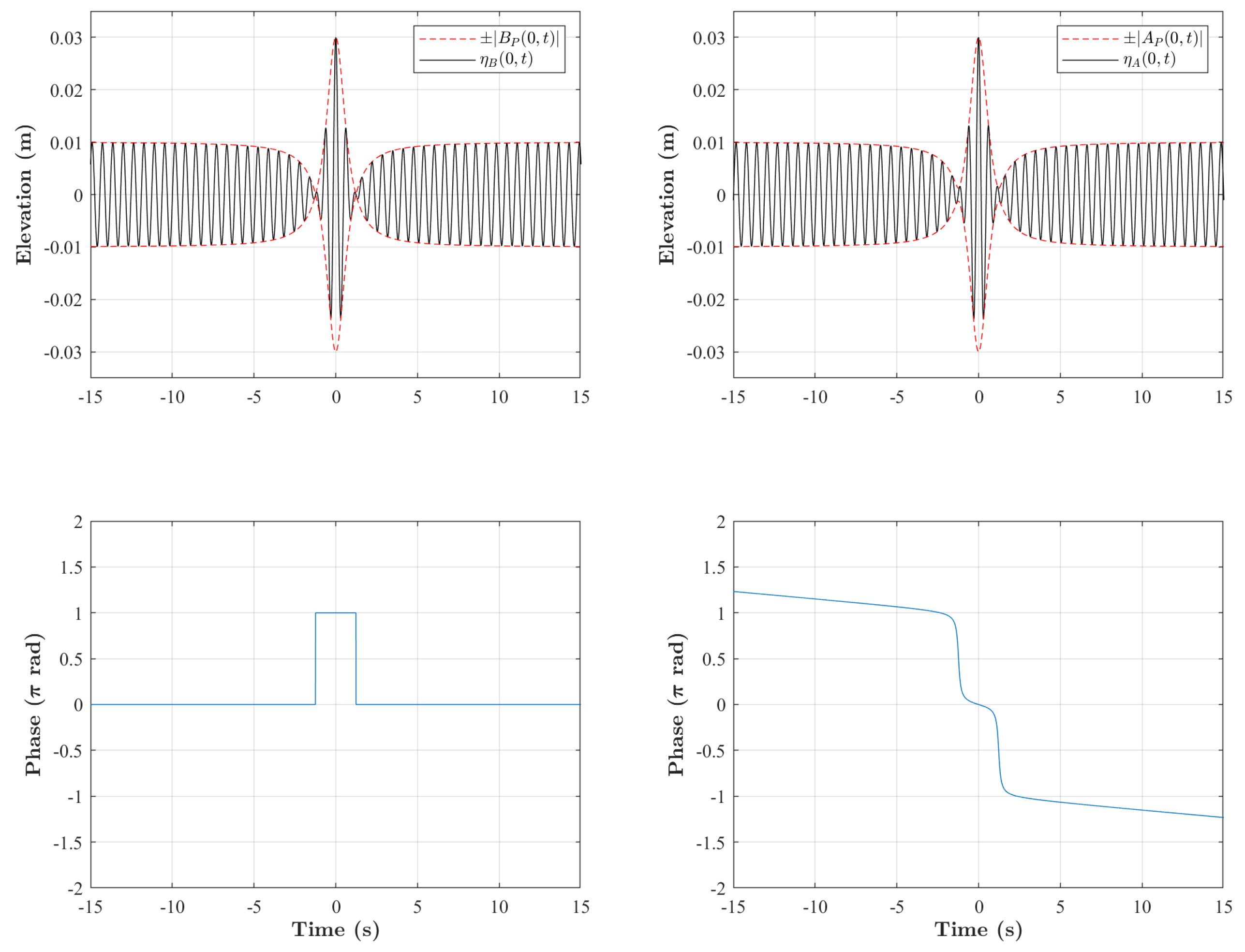
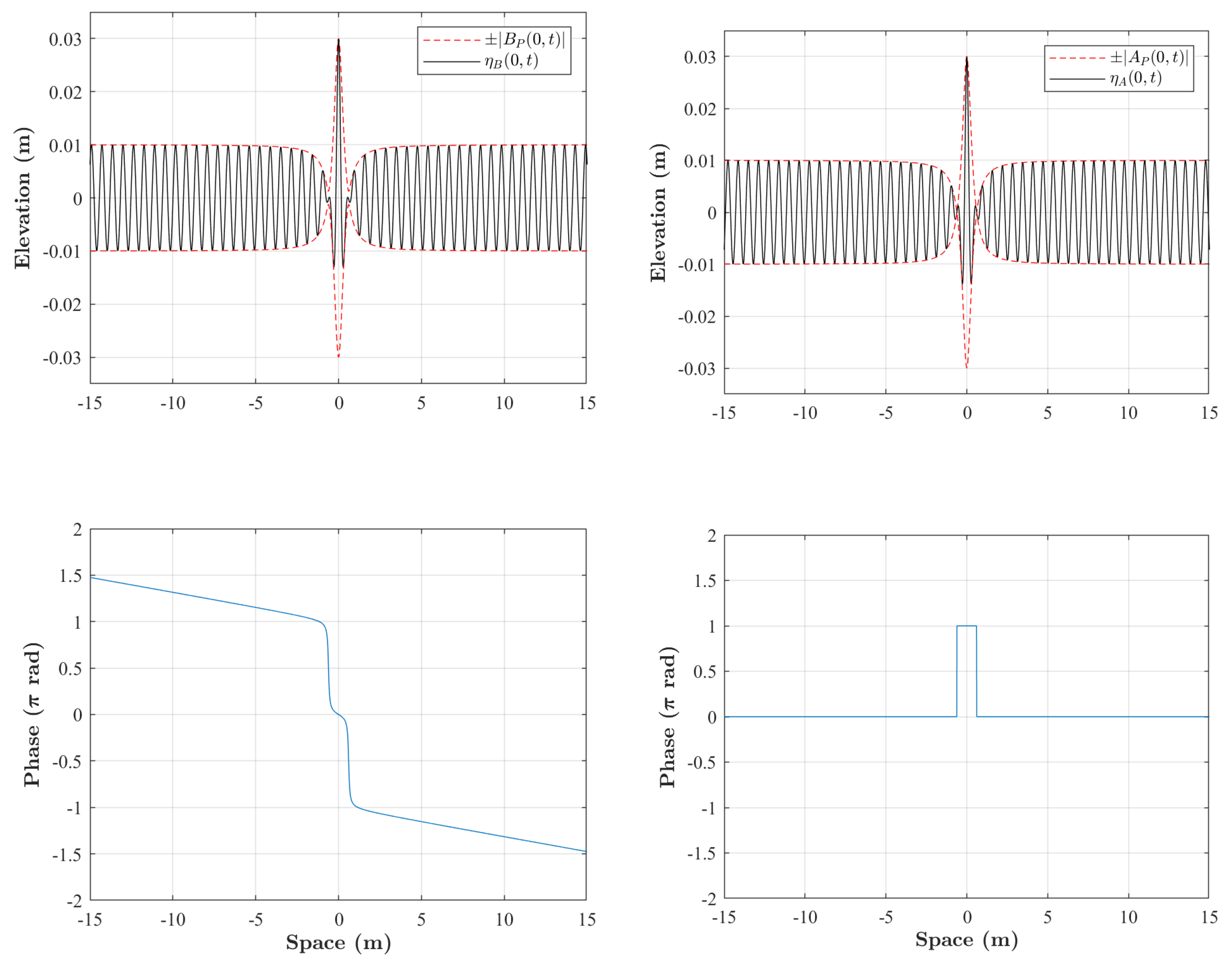
In reference [23], the authors have discussed the differences in the wave envelope propagation of the quasi-identical time- and space-like Peregrine wave group. Here, we will rather focus our attention on the phase evolution, which is different. To initiate our investigation, we will consider the boundary conditions for the two Peregrine models, namely the space-like and time-like formulations, and , respectively, at maximal compression location m and analyze the corresponding phase jumps in the respective temporal profiles. Figure 1 shows both the time-series and the corresponding characteristic phase jump for each of the two cases.
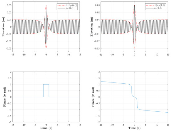
Figure 1.
Theoretical temporal surface elevation profiles (solid black lines), wave envelope (dashed red lines) and the corresponding phase (blue lines) of the Peregrine breather at its peak location m from time-NLSE (left) and space-NLSE (right). The steepness adopted is and the carrier wave amplitude is m. Same parameters have been adopted for the following.
It is noticeable that the phase diagram is different even though the envelope/surface elevation profiles look almost similar. On the other hand, both phases experience a sharp transition of . This motivates a quantitative experimental investigation of the phase evolution when considering one boundary condition or the other to investigate the physical relevance of breather models. Interestingly, when considering the initial conditions of the time- and space-like Peregrine breather at the maximal focusing time s, the same phase jump patterns can be noticed; however, the characteristic phase variations are interchanged compared to the previous case, see Figure 2.
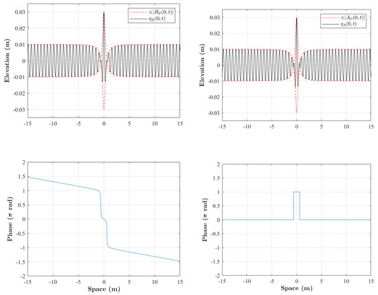
Figure 2.
Theoretical spatial surface elevation profiles (solid black lines), wave envelope (dashed red lines) and the corresponding phase (blue lines) of the Peregrine breather at its peak time s from time-NLSE (left) and space-NLSE (right).
This suggests once again that when using two different boundary conditions to trigger the evolution of the Peregrine breather, the wave envelope may look almost identical in both cases; nevertheless, the characteristic phase-shift dynamics may differ during the propagation.
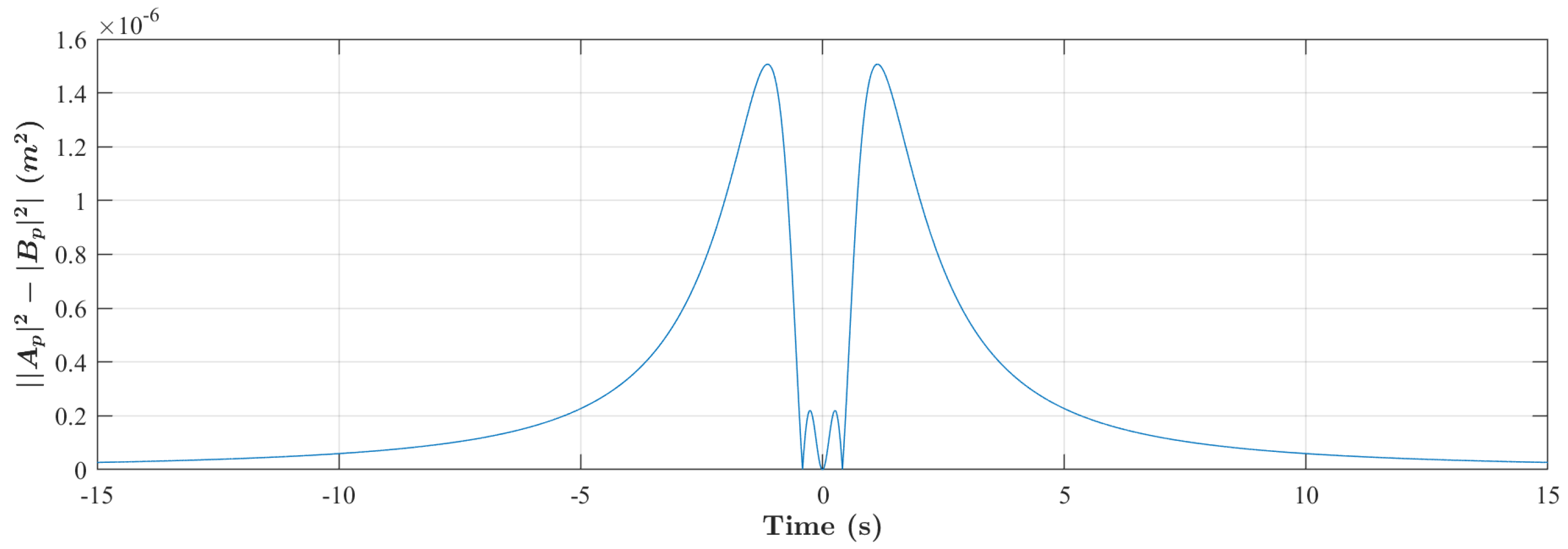
When considering a reasonable choice of carrier steepness below the breaking threshold found to be at 0.12 for the Peregrine breather, the difference in wave amplitude is obviously very small and almost negligible in a laboratory experiment. The difference in intensity for and m at is shown in Figure 3.
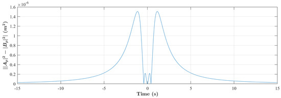
Figure 3.
The absolute value of the intensity difference between the time- and space-like Peregrine breather for the carrier wave parameters and m at m.
The next section elaborates on the experimental investigation.
3. Experimental Investigation
3.1. Experimental Setup
The experiments were carried out in the wave flume of the University of Sydney, which is sketched in Figure 4. The flume has a dimension of 30 × 1 × 1 m3 and an effective water depth of 0.7 m. A piston-type wave maker can generate a variety of waves with frequencies ranging from 0.4 to 2 Hz. An inclined slope covered with artificial grass is installed at the opposite end to absorb the wave energy, allowing a uni-directional investigation of the wave field. The setup and wave parameters chosen ensure that the effects of wave reflections are negligible and do not interfere with the evolution of the Peregrine breather.
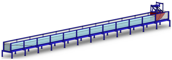
Figure 4.
Wave flume setup and sketch, as installed at the University of Sydney.
In the current experiments, the steepness of the initial condition is set to be 0.1, which is moderate and below the breaking threshold [22,36]. The amplitude of the carrier wave here is selected to be m. These two key parameters are sufficient to determine the wavenumber m−1, wave frequency s−1 and the frequency Hz. The parameters chosen allow the clean observation of the growth and decay of the Peregrine breather in the flume, while the steepness can be regarded as a scaling factor in the modeling [36]. In this case, the dimensionless depth is , which satisfies the deep-water regime. During the experiment, the two adopted boundary conditions of the Peregrine breather and have been defined at m. These parameters facilitate the start of the breather dynamics from a small perturbation of the carrier wave. Eight calibrated wave gauges have been deployed along the wave facility to record the Peregrine breather compression and attenuation. Both Peregrine water surface elevations and corresponding local phase evolutions in the acquired data will be compared with respective theoretical predictions in the next subsection.
3.2. Evolution of the Time- and Space-Like Peregrine Breather in a Water Wave Flume
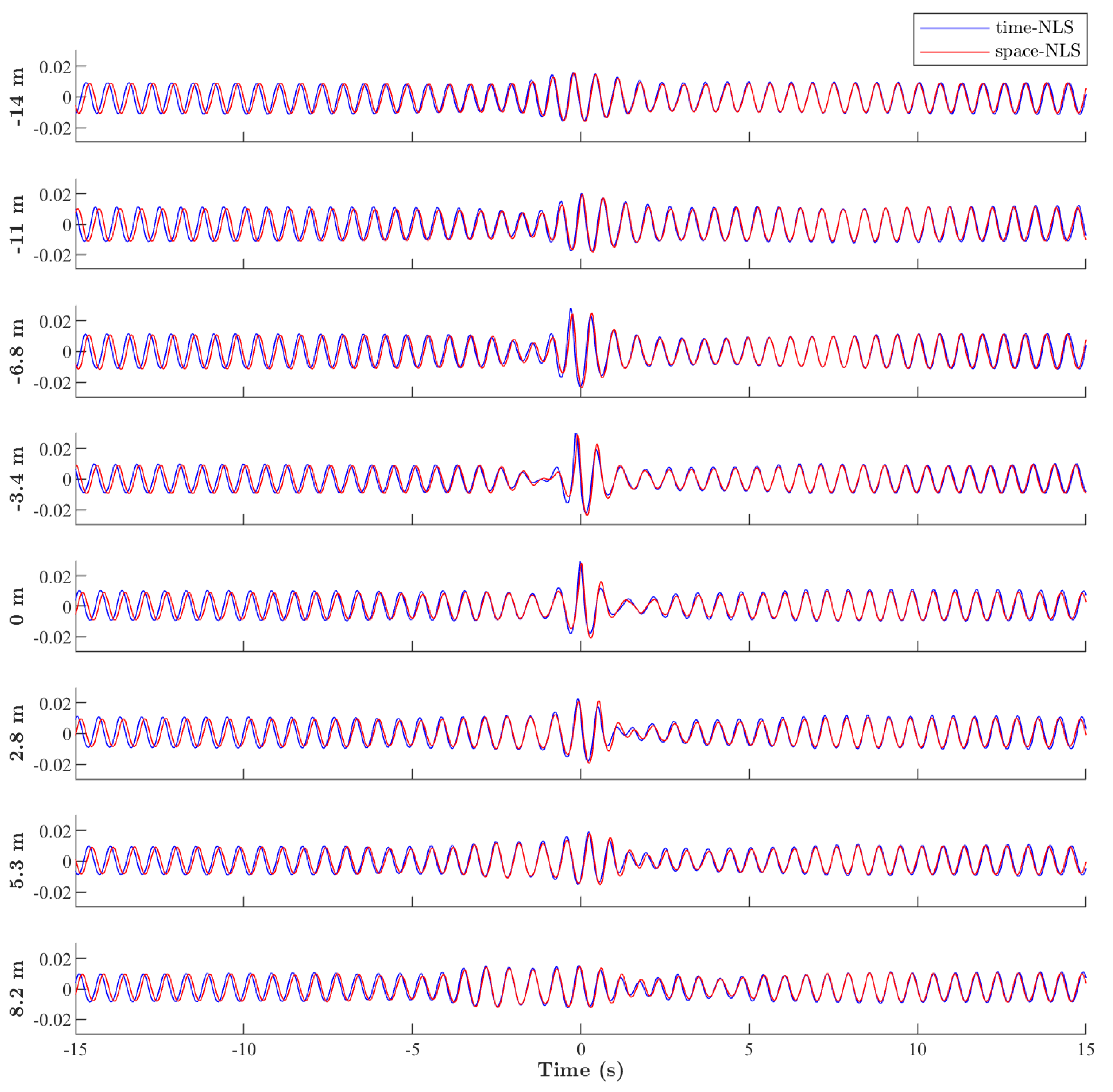
As already described in [5,6], once the wave maker is programmed to generate the exact boundary condition as defined by theory, the experiment consists of recording the temporal evolution of the wave dynamics along the longitudinal direction of the wave flume by the wave gauges. Next, we compare the surface elevation displacements captured by the wave probes when the boundary condition has been determined following the time- and space-like NLSE frameworks. Moreover, to gain an improved quantitative understanding of the expected phase discrepancy in the evolution of both Peregrine wave fields, the wave profiles at gauge location have been superimposed. The results are shown in Figure 5.
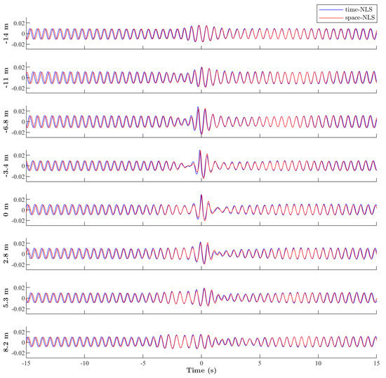
Figure 5.
Superposition and comparison of measured Peregrine hydrodynamics along the wave tank for , m and m and according to the time-like (blue lines) and space-like NLSE (red lines) frameworks.
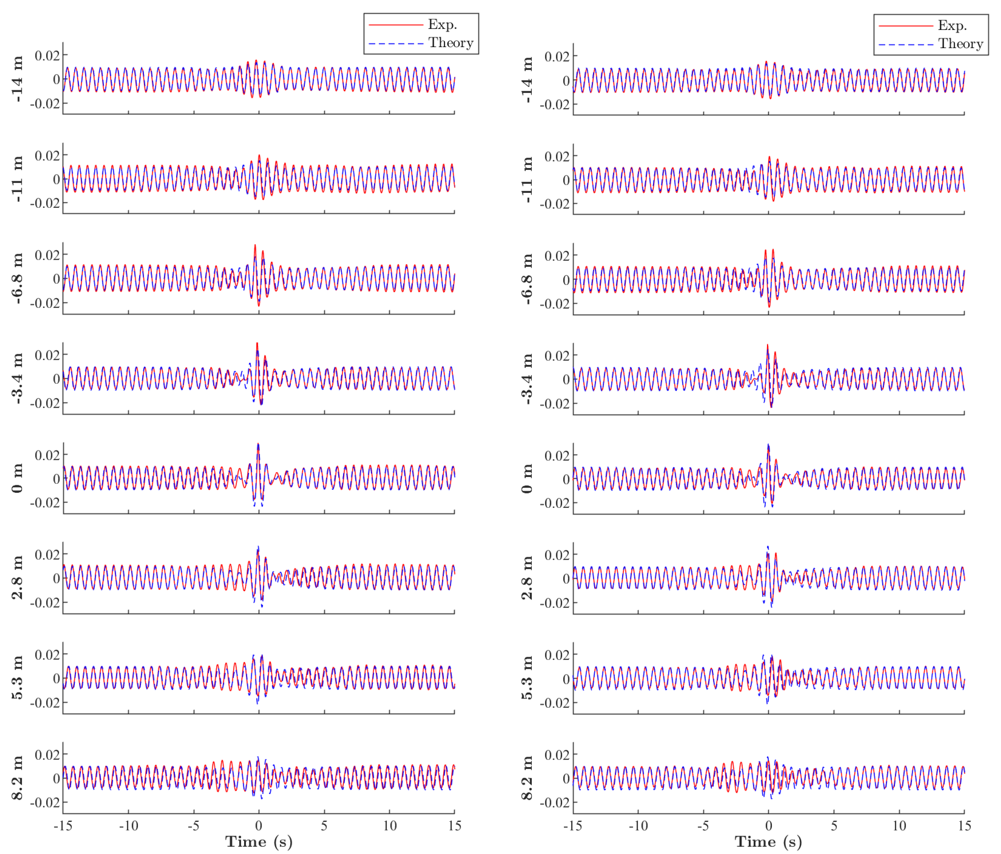
Both Peregrine breather observations were also compared with the corresponding theoretical frameworks, as shown in Figure 6.
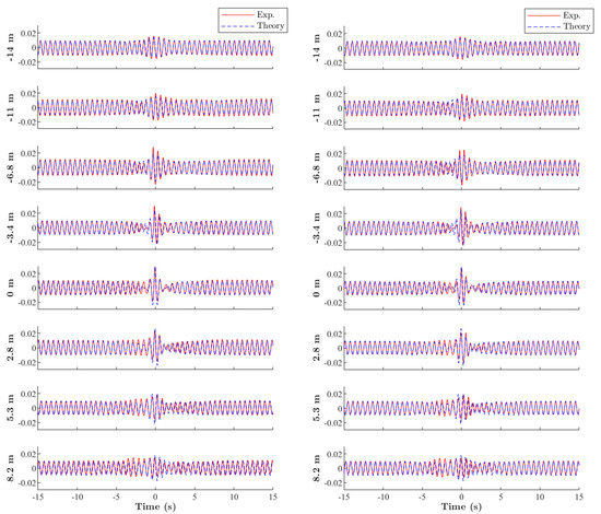
Figure 6.
The experimental measurements compared with the corresponding theoretical predictions for the time- (left) and space-like (right) Peregrine breather solution.
At first view, both envelopes in Figure 5 undergo the same evolution, but there is a distinct phase mismatch, which is obvious when focusing the attention on the generic Peregrine localization. Moreover, the breather undergoes a gradual asymmetric compression, which affects the NLSE comparison accuracy. It is well-known that these are well-captured in higher-order NLSE-type evolution equations and can be tamed by reducing the wave steepness [22,37,38,39]. Since it is not possible to significantly reduce the carrier amplitude, the reduction of wave steepness can be achieved by increasing the wave frequency. However, the increase in the wavelength shortens the effective evolution of the breather in the facility, limited to a total physical propagation distance of 25 m.
On the other hand, it becomes clear that locally, and around the packet, the surface elevation is almost identical, and gradual disagreement in the carrier phase can be observed, affirming a difference in the phase evolution while both envelope amplitudes remain almost identical.
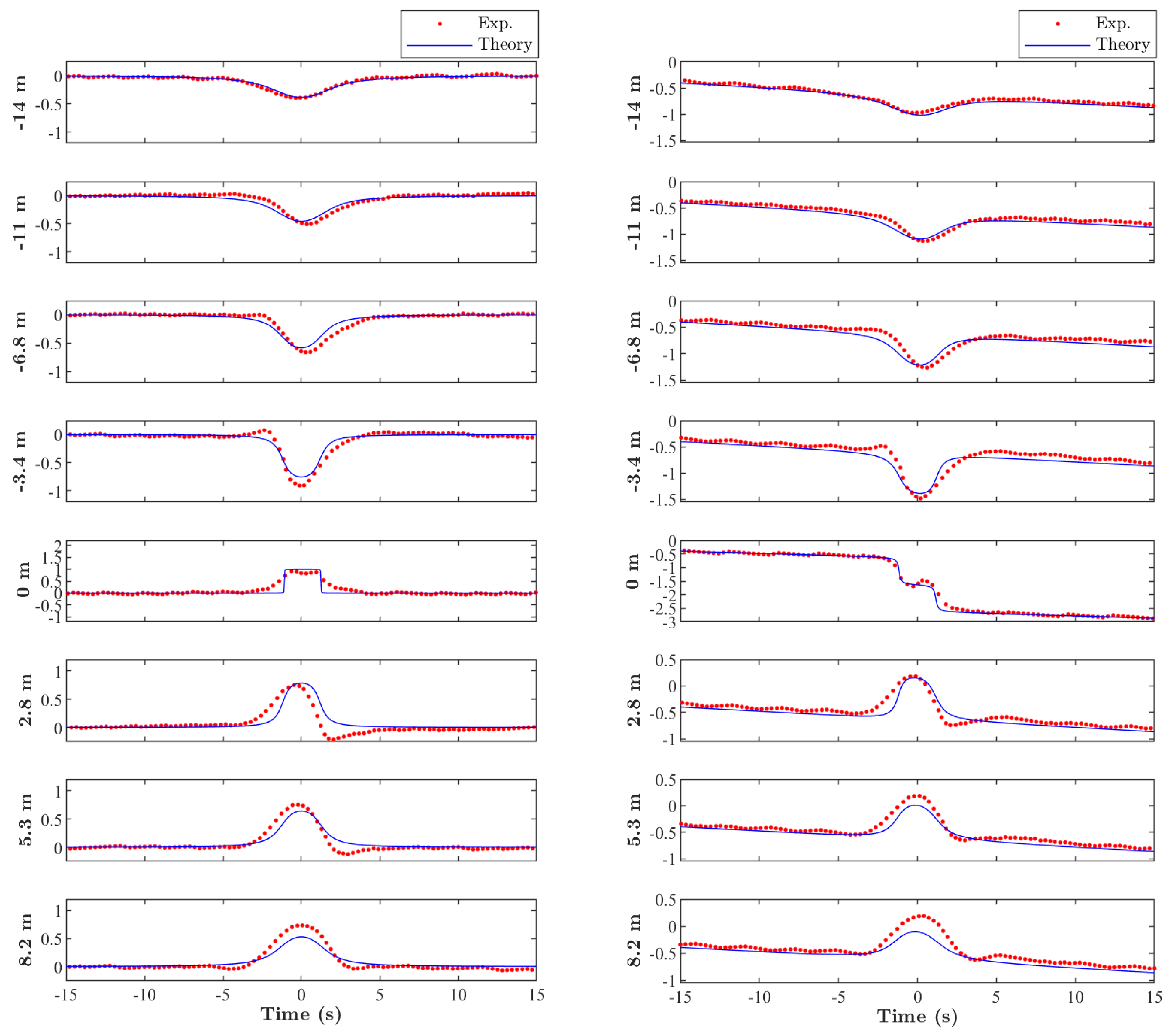
Next, we track the evolution of the phases along the water wave tank for each of the two runs. We recall that the reconstruction of the phase profiles can be achieved using the Hilbert transform according to Equation (16) and as described in [2]. Note that we are computing the phase variations from the water surface measurements by adopting a symmetric truncation around the wave packet. Figure 7 shows the results.
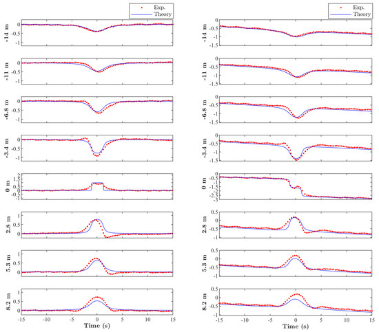
Figure 7.
Experimental (red dots) and theoretical (blue lines) phase evolution along the wave tank corresponding to the surface evolution measurements of Figure 5 for the time-NLSE (left) and space-NLSE (right).
Interestingly, despite the fact the phase evolution in Figure 7 differs from one case to the other, there is clear agreement with the underlying time- or space-like NLSE framework prediction. The differences in the jump at the maximal compression location, i.e., , are responsible for the mismatch in the surface elevation profiles, as can be seen in Figure 5. The discrepancies with NLSE theory already observed in the water surface profiles can be also observed in the evolution of phase profiles, in which deviations are more pronounced after the strong focusing of the breather. This sheds new light on the Peregrine breather dynamics, which can evolve in two different ways. While the envelope amplitudes are quasi-similar, the phase dynamics are distinct. This feature suggests, for instance, alternatives in the identification from phase-shift profiles.
4. Discussion and Conclusions
We have experimentally investigated the phase evolution of Peregrine breather hydrodynamics, which have been initiated by two different boundary conditions as defined by the time- and space-like NLSE framework, respectively. Both envelope expressions being asymptotically equivalent, it is shown in the experiments that despite the almost identical envelope amplitude evolution and the local agreement of the carrier phases around the perturbed wave packet, the global phase dynamics differs. This suggests that two different phase evolutions are possible for such doubly localized rogue wave dynamics. These phase jumps, as identified and tracked along the propagation distance in the experiments, are in agreement with the theoretical prediction as provided by the respective time- or space-NLSE framework. These results provide a new fundamental insight into Peregrine breather-type wave group dynamics and might be, for instance, useful in the development of detection mechanisms for extreme events in nonlinear dispersive media, which form as a result of four-wave interactions.
Author Contributions
Conducting the experiments, Y.H.; all authors contributed equally to the rest of the work. All authors have read and agreed to the published version of the manuscript.
Funding
This research was funded by the University of Sydney for the International Strategic Scholarship (USydIS) and the Ministry of Higher Education and Research, Hauts de France council; Agence Nationale de la Recherche (CEMPI ANR-11-LABX-0007, DYDICO ANR-16-IDEX-0004).
Data Availability Statement
Data will be made available upon reasonable request.
Acknowledgments
P.S. acknowledges Stephane Randoux and Francois Copie for fruitful discussions. A.C. thanks Roger H. J. Grimshaw for the continuous and inspiring communication.
Conflicts of Interest
The authors declare no conflict of interest.
References
- Kharif, C.; Pelinovsky, E.; Slunyaev, A. Rogue Waves in the Ocean; Springer Science & Business Media: New York, NY, USA, 2008. [Google Scholar]
- Osborne, A. Nonlinear Ocean Waves and the Inverse Scattering Transform; Academic Press: New York, NY, USA, 2010; Volume 97. [Google Scholar]
- Agrawal, G. Nonlinear Fiber Optics; Optics and Photonics; Elsevier Science: Amsterdam, The Netherlands, 2013. [Google Scholar]
- Dudley, J.M.; Dias, F.; Erkintalo, M.; Genty, G. Instabilities, breathers and rogue waves in optics. Nat. Photonics 2014, 8, 755–764. [Google Scholar] [CrossRef]
- Onorato, M.; Residori, S.; Bortolozzo, U.; Montina, A.; Arecchi, F. Rogue waves and their generating mechanisms in different physical contexts. Phys. Rep. 2013, 528, 47–89. [Google Scholar] [CrossRef]
- Chabchoub, A.; Hoffmann, N.; Akhmediev, N. Rogue wave observation in a water wave tank. Phys. Rev. Lett. 2011, 106, 204502. [Google Scholar] [CrossRef] [PubMed]
- Kibler, B.; Fatome, J.; Finot, C.; Millot, G.; Dias, F.; Genty, G.; Akhmediev, N.; Dudley, J.M. The Peregrine soliton in nonlinear fibre optics. Nat. Phys. 2010, 6, 790–795. [Google Scholar] [CrossRef]
- Walczak, P.; Randoux, S.; Suret, P. Optical Rogue Waves in Integrable Turbulence. Phys. Rev. Lett. 2015, 114, 143903. [Google Scholar] [CrossRef] [PubMed]
- Suret, P.; El Koussaifi, R.; Tikan, A.; Evain, C.; Randoux, S.; Szwaj, C.; Bielawski, S. Single-shot observation of optical rogue waves in integrable turbulence using time microscopy. Nat. Commun. 2016, 7, 13136. [Google Scholar] [CrossRef] [Green Version]
- Tikan, A.; Billet, C.; El, G.; Tovbis, A.; Bertola, M.; Sylvestre, T.; Gustave, F.; Randoux, S.; Genty, G.; Suret, P.; et al. Universality of the Peregrine soliton in the focusing dynamics of the cubic nonlinear Schrödinger equation. Phys. Rev. Lett. 2017, 119, 033901. [Google Scholar] [CrossRef] [Green Version]
- Wang, R.; Balachandran, B. Extreme wave formation in unidirectional sea due to stochastic wave phase dynamics. Phys. Lett. A 2018, 382, 1864–1872. [Google Scholar] [CrossRef]
- Tikan, A.; Bielawski, S.; Szwaj, C.; Randoux, S.; Suret, P. Single-shot measurement of phase and amplitude by using a heterodyne time-lens system and ultrafast digital time-holography. Nat. Photonics 2018, 12, 228–234. [Google Scholar] [CrossRef]
- Dudley, J.M.; Genty, G.; Mussot, A.; Chabchoub, A.; Dias, F. Rogue waves and analogies in optics and oceanography. Nat. Rev. Phys. 2019, 1, 675–689. [Google Scholar] [CrossRef]
- Tikan, A. Effect of local Peregrine soliton emergence on statistics of random waves in the one-dimensional focusing nonlinear Schrödinger equation. Phys. Rev. E 2020, 101, 012209. [Google Scholar] [CrossRef] [PubMed] [Green Version]
- Hasimoto, H.; Ono, H. Nonlinear modulation of gravity waves. J. Phys. Soc. Jpn. 1972, 33, 805–811. [Google Scholar] [CrossRef]
- Mei, C.C.; Stiassnie, M.; Yue, D.K.P. Theory and Applications of Ocean Surface Waves: Nonlinear Aspects; World Scientific: Singapore, 2005; Volume 23. [Google Scholar]
- Ablowitz, M.J. Nonlinear Dispersive Waves: Asymptotic Analysis and Solitons; Cambridge University Press: Cambridge, UK, 2011; Volume 47. [Google Scholar]
- Zakharov, V.E. Stability of periodic waves of finite amplitude on the surface of a deep fluid. J. Appl. Mech. Tech. Phys. 1968, 9, 190–194. [Google Scholar] [CrossRef]
- Ducrozet, G.; Bonnefoy, F.; Le Touzé, D.; Ferrant, P. A modified high-order spectral method for wavemaker modeling in a numerical wave tank. Eur. J. Mech.-B/Fluids 2012, 34, 19–34. [Google Scholar] [CrossRef]
- Chabchoub, A.; Mozumi, K.; Hoffmann, N.; Babanin, A.V.; Toffoli, A.; Steer, J.N.; van den Bremer, T.S.; Akhmediev, N.; Onorato, M.; Waseda, T. Directional soliton and breather beams. Proc. Natl. Acad. Sci. USA 2019, 116, 9759–9763. [Google Scholar] [CrossRef] [Green Version]
- Slunyaev, A.; Pelinovsky, E.; Sergeeva, A.; Chabchoub, A.; Hoffmann, N.; Onorato, M.; Akhmediev, N. Super-rogue waves in simulations based on weakly nonlinear and fully nonlinear hydrodynamic equations. Phys. Rev. E 2013, 88, 012909. [Google Scholar] [CrossRef] [Green Version]
- Shemer, L.; Alperovich, L. Peregrine breather revisited. Phys. Fluids 2013, 25, 051701. [Google Scholar] [CrossRef] [Green Version]
- Chabchoub, A.; Grimshaw, R.H. The hydrodynamic nonlinear Schrödinger equation: Space and time. Fluids 2016, 1, 23. [Google Scholar] [CrossRef] [Green Version]
- Akhmediev, N.; Eleonskii, V.; Kulagin, N. Generation of periodic trains of picosecond pulses in an optical fiber: Exact solutions. Sov. Phys. JETP 1985, 62, 894–899. [Google Scholar]
- Houtani, H.; Waseda, T.; Tanizawa, K. Experimental and numerical investigations of temporally and spatially periodic modulated wave trains. Phys. Fluids 2018, 30, 034101. [Google Scholar] [CrossRef]
- Peregrine, D.H. Water waves, nonlinear Schrödinger equations and their solutions. ANZIAM J. 1983, 25, 16–43. [Google Scholar] [CrossRef] [Green Version]
- Kedziora, D.J.; Ankiewicz, A.; Akhmediev, N. The phase patterns of higher-order rogue waves. J. Opt. 2013, 15, 064011. [Google Scholar] [CrossRef]
- Xu, G.; Hammani, K.; Chabchoub, A.; Dudley, J.M.; Kibler, B.; Finot, C. Phase evolution of Peregrine-like breathers in optics and hydrodynamics. Phys. Rev. E 2019, 99, 012207. [Google Scholar] [CrossRef] [Green Version]
- Bailung, H.; Sharma, S.; Nakamura, Y. Observation of Peregrine solitons in a multicomponent plasma with negative ions. Phys. Rev. Lett. 2011, 107, 255005. [Google Scholar] [CrossRef]
- Randoux, S.; Suret, P.; Chabchoub, A.; Kibler, B.; El, G. Nonlinear spectral analysis of Peregrine solitons observed in optics and in hydrodynamic experiments. Phys. Rev. E 2018, 98, 022219. [Google Scholar] [CrossRef] [Green Version]
- Wang, J.; Ma, Q.; Yan, S.; Chabchoub, A. Persistence of Peregrine Breather in Random Sea States. Phys. Rev. Appl. 2018, 9, 014016. [Google Scholar] [CrossRef]
- Michel, G.; Bonnefoy, F.; Ducrozet, G.; Prabhudesai, G.; Cazaubiel, A.; Copie, F.; Tikan, A.; Suret, P.; Randoux, S.; Falcon, E. Emergence of Peregrine solitons in integrable turbulence of deep water gravity waves. Phys. Rev. Fluids 2020, 5, 082801. [Google Scholar] [CrossRef]
- Shabat, A.; Zakharov, V. Exact theory of two-dimensional self-focusing and one-dimensional self-modulation of waves in nonlinear media. Sov. Phys. JETP 1972, 34, 62. [Google Scholar]
- Akhmediev, N.N.; Ankiewicz, A. Solitons: Nonlinear Pulses and Beams; Chapman & Hall: London, UK, 1997. [Google Scholar]
- Shrira, V.I.; Geogjaev, V.V. What makes the Peregrine soliton so special as a prototype of freak waves? J. Eng. Math. 2010, 67, 11–22. [Google Scholar] [CrossRef]
- Chabchoub, A.; Akhmediev, N.; Hoffmann, N. Experimental study of spatiotemporally localized surface gravity water waves. Phys. Rev. E 2012, 86, 016311. [Google Scholar] [CrossRef] [Green Version]
- Dysthe, K.B. Note on a modification to the nonlinear Schrödinger equation for application to deep water waves. Proc. R. Soc. Lond. A Math. Phys. Sci. 1979, 369, 105–114. [Google Scholar]
- Trulsen, K.; Dysthe, K.B. A modified nonlinear Schrödinger equation for broader bandwidth gravity waves on deep water. Wave Motion 1996, 24, 281–289. [Google Scholar] [CrossRef]
- Waseda, T.; Fujimoto, W.; Chabchoub, A. On the Asymmetric Spectral Broadening of a Hydrodynamic Modulated Wave Train in the Optical Regime. Fluids 2019, 4, 84. [Google Scholar] [CrossRef] [Green Version]

Publisher’s Note: MDPI stays neutral with regard to jurisdictional claims in published maps and institutional affiliations. |
© 2021 by the authors. Licensee MDPI, Basel, Switzerland. This article is an open access article distributed under the terms and conditions of the Creative Commons Attribution (CC BY) license (https://creativecommons.org/licenses/by/4.0/).