Article

A Computational Fluid Dynamics Model for the Small-Scale Dynamics of Wave, Ice Floe and Interstitial Grease Ice Interaction

1
Department of Civil Engineering, University of Cape Town, Cape Town 7700, South Africa
2
Marine and Antarctic Research Centre for Innovation and Sustainability, University of Cape Town, Cape Town 7700, South Africa
3
Ex Mente Technologies, Pretoria 0081, South Africa
4
School of Computer Science and Applied Mathematics, University of Witwatersrand, Johannesburg 2000, South Africa
5
Graduate School of Frontier Sciences, The University of Tokyo, Tokyo 113-8654, Japan
6
Department of Infrastructure Engineering, University of Melbourne, Parkville, VIC 3010, Australia
7
Institute of Mechanics, University of Duisburg-Essen, 47057 Duisburg, Germany
8
Department of Oceanography, University of Cape Town, Cape Town 7700, South Africa
*
Authors to whom correspondence should be addressed.
Fluids 2021, 6(5), 176; https://doi.org/10.3390/fluids6050176
Submission received: 30 March 2021 / Revised: 21 April 2021 / Accepted: 23 April 2021 / Published: 29 April 2021
(This article belongs to the Special Issue Mathematical and Numerical Modeling of Water Waves)

Abstract

:
The marginal ice zone is a highly dynamical region where sea ice and ocean waves interact. Large-scale sea ice models only compute domain-averaged responses. As the majority of the marginal ice zone consists of mobile ice floes surrounded by grease ice, finer-scale modelling is needed to resolve variations of its mechanical properties, wave-induced pressure gradients and drag forces acting on the ice floes. A novel computational fluid dynamics approach is presented that considers the heterogeneous sea ice material composition and accounts for the wave-ice interaction dynamics. Results show, after comparing three realistic sea ice layouts with similar concentration and floe diameter, that the discrepancy between the domain-averaged temporal stress and strain rate evolutions increases for decreasing wave period. Furthermore, strain rate and viscosity are mostly affected by the variability of ice floe shape and diameter.

1. Introduction

The region where ocean processes affect sea ice, known as marginal ice zone (MIZ; [1]), is a highly complex system [2,3,4] particularly during the ice formation and melt season. Most contemporary dynamic-thermodynamic sea ice models used for predicting global climate are phenomenological large-scale models (order of 100 km [5]) in which internal stresses are related to the strain rate via a viscous-plastic rheology [6,7,8]. These models adopt a smeared approach in which an area with heterogeneous ice characteristics (fractures, leads, open water and different ice types) is modelled as a single homogeneous material with averaged properties, and in which ice-ocean interactions are parameterised [9]. The dynamics is governed by the momentum balance equation and two continuity equations controlling ice thickness and concentration, accounting for deformation and growth-related effects [10]. However, sea ice deformation cannot be exclusively described by a viscous-plastic rheology as sea ice drift on the scale of less than 10 km is only accurate to a certain extent and fails to reproduce sea ice deformation at finer scales [11,12].
The MIZ is regulated by both large- and small-scale processes. Large-scale processes, on a spatial scale of 100 km and a temporal scale of several days, are the Coriolis force and large-scale ocean circulation [13,14]. Fine-scale processes, on the scale of hours and less than 10 km, are the variability in the sea ice cover and stress acting at the air-ocean-ice interface [15,16]. Among small-scale processes in the Antarctic MIZ, waves play a crucial role in the formation of sea ice [17,18]. Furthermore, the propagation of waves from open ocean into the MIZ and wave-ice interaction are linked to wave scattering and dissipation through the momentum transfer to ice floes, which mainly depend on sea ice characteristics like ice floe geometry and floe size distribution [19]. In particular, at the ice edge, close to the open ocean, high energy incident waves create complicated sea states resulting in violent ice floe motion and collision [17,20]. During the Antarctic winter, when temperatures are low, sea ice initially forms as small circular floes [21,22,23] (1–10 m in diameter, smaller than the characteristic wavelength), known as pancakes, surrounded by grease ice under the action of ocean waves penetrating deep into the ice covered ocean [24,25].
Dynamic-thermodynamic sea ice models on a floe-scale are scarce [12], in particular with respect to the characteristic pancake ice floes found in the winter MIZ. Most of the existing fine-scale numerical models are based on a molecular dynamics schemes based on Hertzian collision dynamics [21,26,27] that consider sea ice physics and dynamics at a floe level [28]. The Discrete-Element bonded-particle model by Herman et al. [29] highlights the significance of skin drag on wave attenuation and floe collision dynamics due to prolonged collision and reduced restitution coefficient. The model uses an heuristic contact detection algorithm and includes simplified overwash (water overflowing the ice [30,31,32]), and elastic and inelastic contact force contributions, with the latter linked to the restitution coefficient; tangential friction is not accounted for. Damsgaard et al. [33] uses a discrete element framework for the approximation of Lagrangian sea ice dynamics also at the floe level. The modelling of fragmented sea ice in the MIZ is improved by using exact solutions for mechanical nonlinearities with arbitrary sea ice concentrations. Rabatel et al. [34] describes the dynamics of an assembly of rigid ice floes using an event-driven algorithm [35]. Their approach focuses on collisions of individual ice floes of both, arbitrary size and shape derived from satellite images from the Arctic. Ice classified as “new ice” of recently frozen sea water that is not solid ice yet, such as grease ice, has not been considered in these models. Moreover, with the exception of Rabatel et al. [34], all other models have in common the limitation of using highly simplified ice floe shapes.
This paper introduces a novel computational framework, developed using the computational fluid dynamics (CFD) software OpenFOAM (https://www.openfoam.com/ (accessed on 23 April 2021)), for the small-scale wave-ice interaction dynamics. The governing equations for the small-scale model are introduced in Section 2 and the numerical implementation in Section 3. We focus on the pancake and grease ice rheology variables over short time periods (<1 min), during which thermodynamic effects on ice thickness and concentration are negligible and ice floe ridging can be disregarded. We demonstrate the suitability of the proposed computational framework for modelling the elastic collision dynamics of free-floating ice floes embedded in interstitial grease ice under the action of ocean waves by providing a convergence analysis with regards to the domain grid refinement and the sea ice layout in Section 4. We show that the dynamics depends on (i) ice characteristics, (ii) sea ice rheology and (iii) external forcing. With these findings at hand, an initial investigation of realistic ice floe distributions is undertaken in Section 5, focusing on the inter-dependency of floe size and shape, wave forcing and grease ice viscosity. The numerical results are discussed in Section 6 and conclusions are presented in Section 7.

2. Small-Scale Model

2.1. Momentum Equation

The sea ice dynamics is governed by the momentum balance equation
m U t + ( U · ) U = τ a + τ o + τ w + · σ ,
where U represents the sea ice velocity vector and t the time. The mass of ice per area is indicated by m, given as
m = ρ h ,
where ρ is the ice density and h the ice thickness. The internal ice reaction forces are represented by the Cauchy stress tensor, σ , depending on the respective ice constituent. External forcing in terms of in-plane wind and ocean current stress vectors applied to the ice is represented by τ a and τ o , respectively. The in-plane stress due to the waves, τ w (also an external forcing), is derived from the linear wave theory [36] and consists of two components:
τ w = τ s d + τ f k ,
where τ s d is the viscous component representing the skin drag acting on the entire ice-ocean interface and τ f k the Froude–Krylov force due to the wave pressure field acting on the ice floe circumference.
The skin drag is given as
τ s d = ρ w C w | U w U | ( ( U w U ) cos θ w + ( U w U ) × k sin θ w ) ,
where ρ w and θ w represent the water density and the ice-ocean turning angle, respectively, k a unit normal vector to the surface of the ice and C w the ice-ocean drag coefficient. The orbital velocity of the water, U w , for monochromatic waves is defined as
U w = U w x U w y U w z = a ω sin ( ω t k x ) 0 a ω cos ( ω t k x ) ,
where x,y and z represent the Cartesian coordinates within the problem domain. x is taken along the main direction of wave propagation and z in the vertical direction, such that the horizontal y-velocity component can be assumed zero. In Equations (5) and (7) a, ω and k represent the wave amplitude, wave frequency and wave number, respectively. The wave frequency and wave number, ω = 2 π / T and k = 2 π / λ , are computed from the wave period T and the wavelength λ using the deep water dispersion relation ω 2 = g k .
The Froude–Krylov force, τ f k , accounts for the horizontal surge force due to the wave-induced pressure acting at the interface between ice floe and water [37]
τ f k = h w p n d z ,
where h w represents the submerged ice floe thickness portion. The unit vector n acts normal to the circumference of the ice floes directed outwards. The wave-induced pressure, p, is written as
p = ρ w g a sin ( ω t k x ) ,
where the gravitational acceleration is denoted as g.
Equations (6) and (7) can be rewritten as [37]
τ f k = n · h w a ω 2 cos ( ω t k x ) .
The form drag acting on the ice floe circumference due velocity differences of floes and surrounding grease ice is implicitly included by the continuum approach comprising both ice constituents enforcing velocity continuity at the interface.
Ocean drag, τ o , at the basal plane of the ice due to relative velocity of the ocean current and the ice is given by
τ o = ρ w C w | U o U | ( ( U o U ) cos θ w + ( U o U ) × k sin θ w ) ,
whereas the wind drag, τ a , on the apical plane by
τ a = ρ a C a | U a | U a cos θ a + k × U a sin θ a .
The variables U a and U o represent the velocities of wind and ocean boundary layers, respectively. The air density, ice-air drag coefficient and wind turning angle are indicated by ρ a , C a and θ a , respectively.

2.2. Sea Ice Rheology

The rheology in the model is based on the material characteristics of each constituent, grease ice and pancake floes, respectively, and each is represented by its own rheological model. Grease ice behaves like a fluid whereas ice floes have a solid-like behaviour. The ice thickness of both is assumed spatially constant, since ice thickness is negligibly small compared to the domain size in lateral direction. As mentioned before, since only small time periods are considered in the model, ice thickness is assumed unaffected by thermodynamic and rafting-related growth and does not vary in time.
The sea ice strain rate tensor, ϵ ˙ , is used in both grease ice and ice floe rheology and is written in terms of the sea ice velocity gradient, U , as
ϵ ˙ = 1 2 ( U + ( U ) T ) .

2.2.1. Grease Ice Rheology

The fluid-like viscous-plastic behaviour of grease ice is modelled applying a viscous-plastic flow rheology similar as proposed by e.g., Thorndike and Rothrock [38] or Hibler [6]
σ g r e a s e = 2 η ϵ ˙ + I ( ζ η ) tr ( ϵ ˙ ) P 2 ,
where P represents the internal grease ice strength that controls its compressibility, ζ and η are strain rate-dependent grease ice viscosities, namely the spherical and deviatoric contributions, respectively. The identity tensor is indicated by I . The main difference to the above mentioned models is the definition of the ice strength parameter as
P = P * h
where P * represents an empirical constant excluding ice growth and concentration effects. Both strain rate-dependent viscosities are coupled via
ζ = P 2 Δ and η = ζ e 2 ,
where the ratio between the in-plane principle axes of the elliptical yield curve is given by parameter, e, and the effective strain rate, Δ , is given by
Δ = ( ( ϵ ˙ 11 2 + ϵ ˙ 22 2 ) ( 1 + e 2 ) + 4 e 2 ϵ ˙ 12 2 + 2 ϵ ˙ 11 ϵ ˙ 22 ( 1 e 2 ) ) 1 / 2 .
The Cartesian components of the symmetric strain rate tensor are denoted by ϵ ˙ 11 , ϵ ˙ 22 and ϵ ˙ 12 , respectively. As the strain rate approaches zero, the viscosity tends to infinity. To address this, a lower limit of the effective strain rate is enforced, i.e., Δ = 2 · 10 7 s 1 [39].
Equation (12) can be, after substitution of Equation (11), written in terms of the velocity gradient, U , as
σ g r e a s e = η ( U + ( U ) T ) + I ( ζ η ) tr ( U ) P 2 .

2.2.2. Ice Floe Rheology

The solid-like material response of ice floes exhibits relatively small deformations and the constitutive behaviour is therefore described using the generalised Hooke’s law
σ f l o e = 2 μ i ϵ + λ i I tr ( ϵ ) ,
where μ i and λ i represent the Lamé constants. Note, as Hooke’s law is a linear function of the strain tensor, ϵ , Equation (11) can be substituted into its linearised form resulting in
σ f l o e n + 1 = σ n + Δ t μ i ( U + ( U ) T ) + λ i I tr ( U ) ,
where n represents the time index discretised with time step Δ t [40].

3. Numerical Implementation

The framework described in Section 2 is implemented in the Computational Fluid Dynamics (CFD) software OpenFOAM, which is based on the finite volume method (FVM) where a continuum body is approximated by a discrete model [41]. The domain is subdivided, by means of a mesh, into a finite number of small control volumes (cells). The volume of fluid (VOF) method is used in OpenFOAM to distinguish between two immiscible and incompressible fluids with the help of the nondimensional parameter α [42,43]. The VOF method used here is the interface advection scheme presented in [42] that enforces a sharp interface between dominantly solid-like pancake ice floes and viscous fluid-like interstitial grease ice. Cells containing exclusively pancake ice or grease ice have α -values of 1 and 0, respectively, and all intermediate values ( 0 < α < 1 ) have no physical interpretation but are needed in FVM which does not allow for discontinuities. The region of 0 < α < 1 should be numerically constrained to the thin interface between the two ice materials.
The velocity field of the sea ice domain due to an imposed wave forcing is only solved for within the horizontal (x,y)-plane. Accordingly, all terms in the momentum balance equation, Equation (1), are normalised by the respective height of pancake and grease ice, resulting in stress values in terms of kg s 2 . Table 1 shows the general parameters used for all simulations in the following. Ice floes and interstitial grease ice are discretised in OpenFOAM with finite volume elements using the least-squares gradient scheme and the Gauss linear divergence scheme for the spatial integration. The first-order Euler implicit method is used for temporal discretisation. The domain boundary is numerically approximated by horizontal zero-gradient boundary conditions leaving the unknown velocity unspecified at the boundary. As the wave forcing is imposed, the boundary condition introduces an error but only to cells directly adjacent to the boundary. It does not affect the velocity field in the inner domain. To overcome this inconsistency the domain is enlarged to exclude undesired boundary effects for the inner domain.
This numerical study exclusively focuses on the mechanics of wave-ice interaction. As such, the effects of ocean and wind currents, τ o and τ a , respectively, are disregarded, setting U o = 0 ms 1 and U a = 0 ms 1 . Accordingly, the orbital wave velocity, U w , is the only driver forcing the mechanical ice response via the Froude–Krylov force (Equation (8)) and the skin drag (Equation (4)). The former acts on the submerged floe circumference, h w , below the grease ice layer and the latter on the entire ice-ocean interface as controlled by the drag coefficient, C w , with constant but different values for both ice floes and grease ice. The turning angle, θ w , is set to zero, as it can be assumed that on small-scale the ocean current drag acts in the same direction as the ocean velocity [44]. As a result, the net-motion in horizontal direction is negligible such that the ice floes do not get in contact with the domain boundary during the short simulation period of 30 s.
As previously mentioned, the form drag acting on the ice floes due to surrounding grease ice is implicitly accounted for by the continuity requirement of the velocity field throughout the domain which is modelled in a continuum fashion. This also governs the interaction between colliding ice floes which resist the collision forces via an elastic stress and strain response. The effective elastic Lamé parameters are estimated based on values characteristic for compacted snow [45] considering the rather soft rim of ice floes due to collision, grinding and grease ice scavenging. The explicit influence of the grease ice viscosity on wave attenuation is commonly not accounted for, because dissipation per wavelength is small (<0.5%) [18], i.e. the wave amplitude remains almost constant within a small domain.
The convergence analysis with regard to grid size and domain size is conducted to find the optimal cell size to be used in the discretisation of FVM (in Section 4.1) and the critical ratio of floe diameter to domain size as linked to the imposed wave forcing (in Section 4.2). Simplified ice layouts are used consisting of randomly distributed disk-shaped pancake ice floes of constant diameter surrounded by grease ice with a temporally and spatially varying viscosity ν 0.04 m 2 s 1 . In the grid size convergence analysis the domain is exposed to a harmonic propagating wave with period T = 18 s ( λ = 506 m ) and amplitude a = 4.8 m , typically encountered in the Antarctic MIZ [3]. In the domain size convergence analysis three different wave forcing scenarios are considered with periods T = 6 s , T = 12 s and T = 20 s (corresponding to λ = 56 m , λ = 225 m and λ = 625 m ) to cover the majority of occurring wave conditions and amplitudes a = 0.5 m , a = 2.1 m and a = 6 m , respectively. The wave parameters are chosen to maintain a constant wave steepness ( a k ) across the considered cases corresponding to storm waves propagating into the MIZ to highlight their effect on heterogeneous sea ice conditions. The time step Δ t = 0.01 s for the Euler implicit method is chosen for all simulations.
To study the high-resolution mechanical response of sea ice due to wave-ice interaction and ice composition in terms of ice type as well as floe shape and diameter in Section 5, three realistic 100 × 100 m 2 -sea ice layouts are extracted from in situ image and video material recorded by stereo cameras of the dynamics of sea ice in the Antarctic MIZ [22]. The images are collected in close vicinity to each other and, therefore, in homogeneous sea ice conditions with only slightly differing sea ice properties in terms of ice floe concentration and median ice floe caliper diameter. The different layouts also help to verify the robustness of the numerical framework with respect to natural variability of the ice floe distribution in the MIZ.
Table 1. General parameters used in all simulations.
ParameterDefinitionValueUnit
h i , g thickness ice floes and grease ice0.8, 0.2 [46]m
h w submerged ice floe thickness0.54m
ρ i , g density ice floes and grease ice918, 930 [3,47,48,49] kg m 3
λ i first Lamé parameter ice floes6.4 × 10 6  [45] N m 2
μ i second Lamé parameter ice floes3.3 × 10 6  [45] N m 2
ρ w water density1026 [13] kg m 3
C w , i ice-ocean drag coefficient ice floes0.005 [50,51]-
C w , g ice-ocean drag coefficient grease ice0.0013 [47]-
θ w ice-ocean turning angle0 [44]
eyield surface axes ratio grease ice2 [39,40,52]-
a k wave steepness0.06 [18,53]-

4. Convergence Analysis

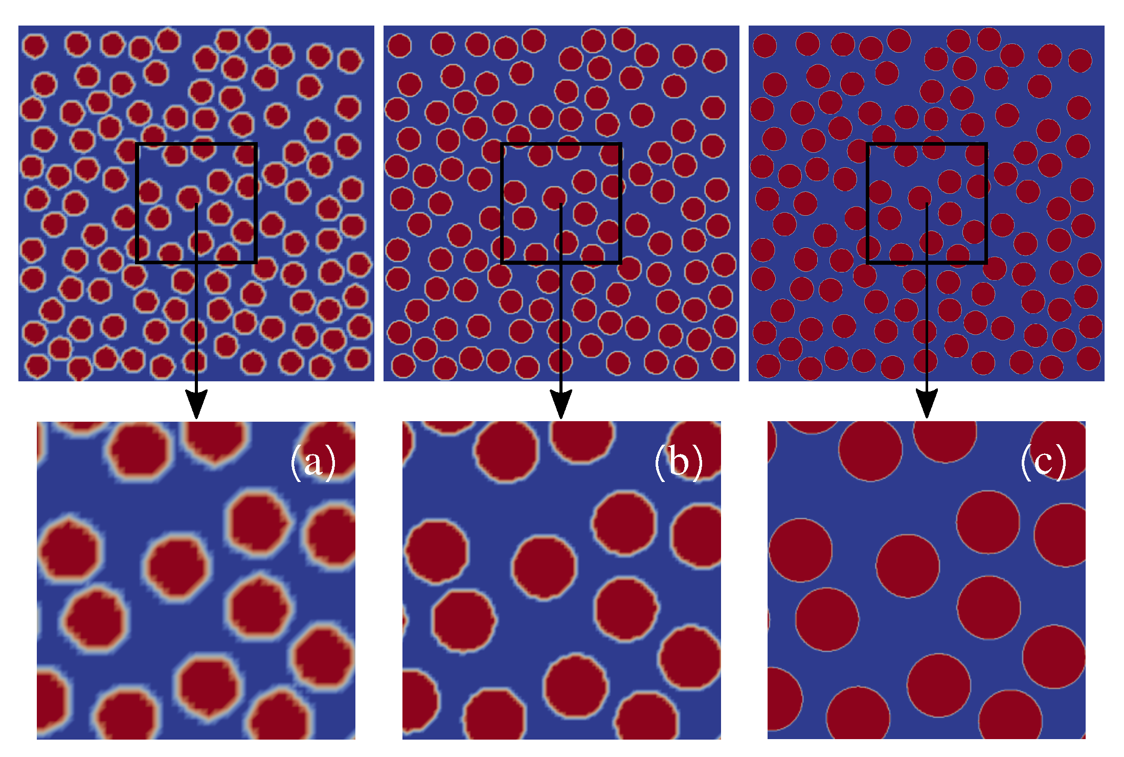
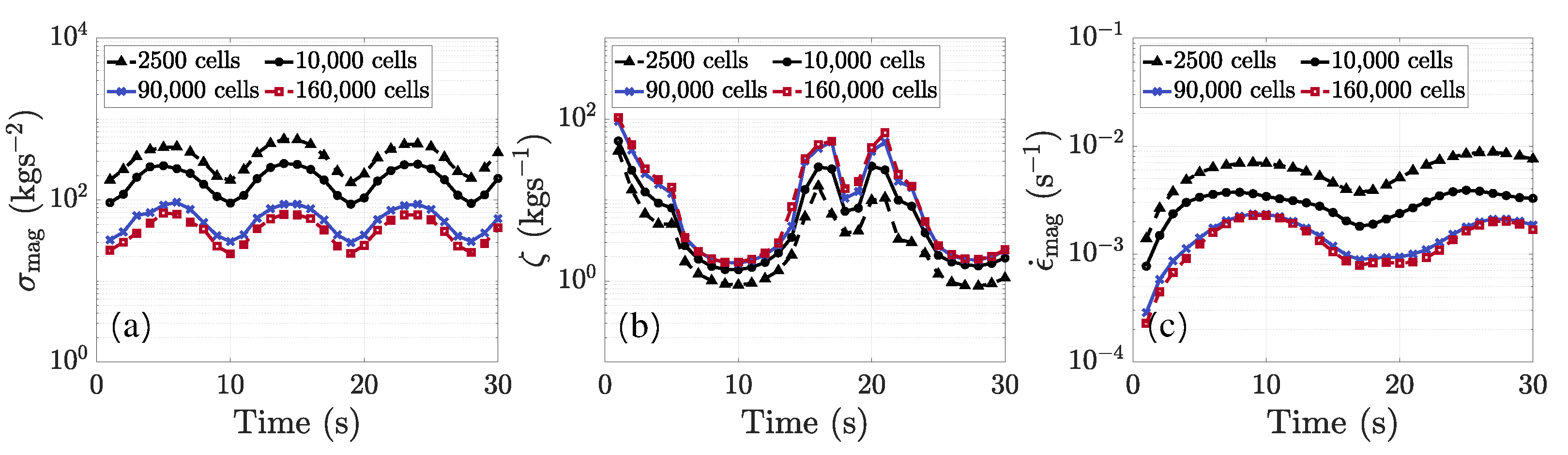
4.1. Grid Size Convergence Analysis

To accurately resolve the interface of pancake floes and the surrounding grease ice, discretisations featuring a higher number of cells provide a sharper boundary as indicated by the white colour in the pancake-grease ice layouts depicted in Figure 1 at t = 0 s . For each discretisation refinement level, the domain-averaged stress and strain rate magnitudes, σ mag = σ i j σ i j and ϵ ˙ mag = ϵ ˙ i j ϵ ˙ i j , as well as the bulk viscosity, ζ , are computed for comparison. σ i j and ϵ ˙ i j represent the Cartesian components of both the stress and strain rate tensor, respectively.
A 100 × 100 m 2 -inner domain size with a 41 % ice floe area fraction is embedded in a 300 × 300 m 2 outer domain to exclude undesired boundary effects for the inner domain, as shown in Figure 1 by the black rectangle. The ice floes have a constant diameter of 20 m . Multiple simulations are carried out, each time with an increasing number of cells in the domain ranging from 2500 to 160,000 cells.
Figure 2 shows the domain-averaged stress, viscosity and strain rate results for the four different grid refinement levels within the 100 × 100 m 2 -inner domain. The blue and red curves, representing 90,000 and 160,000-cell-inner domains, respectively, show similar values indicating convergence. It can be concluded that a total of 90,000 cells for the inner domain, corresponding to a cell size of 0.33 × 0.33 m 2 , is sufficient and will be used for all numerical simulations in the subsequent section.

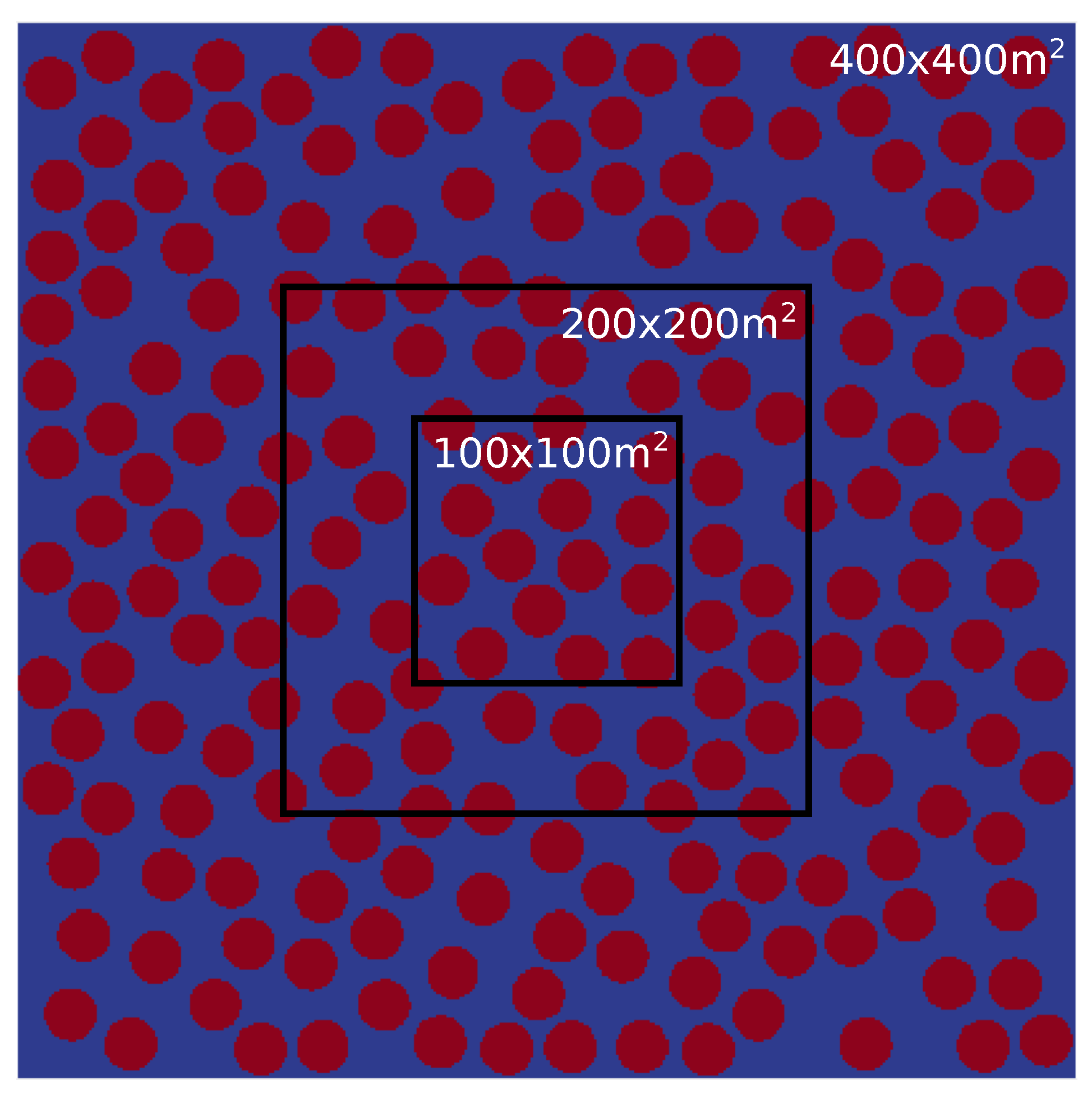
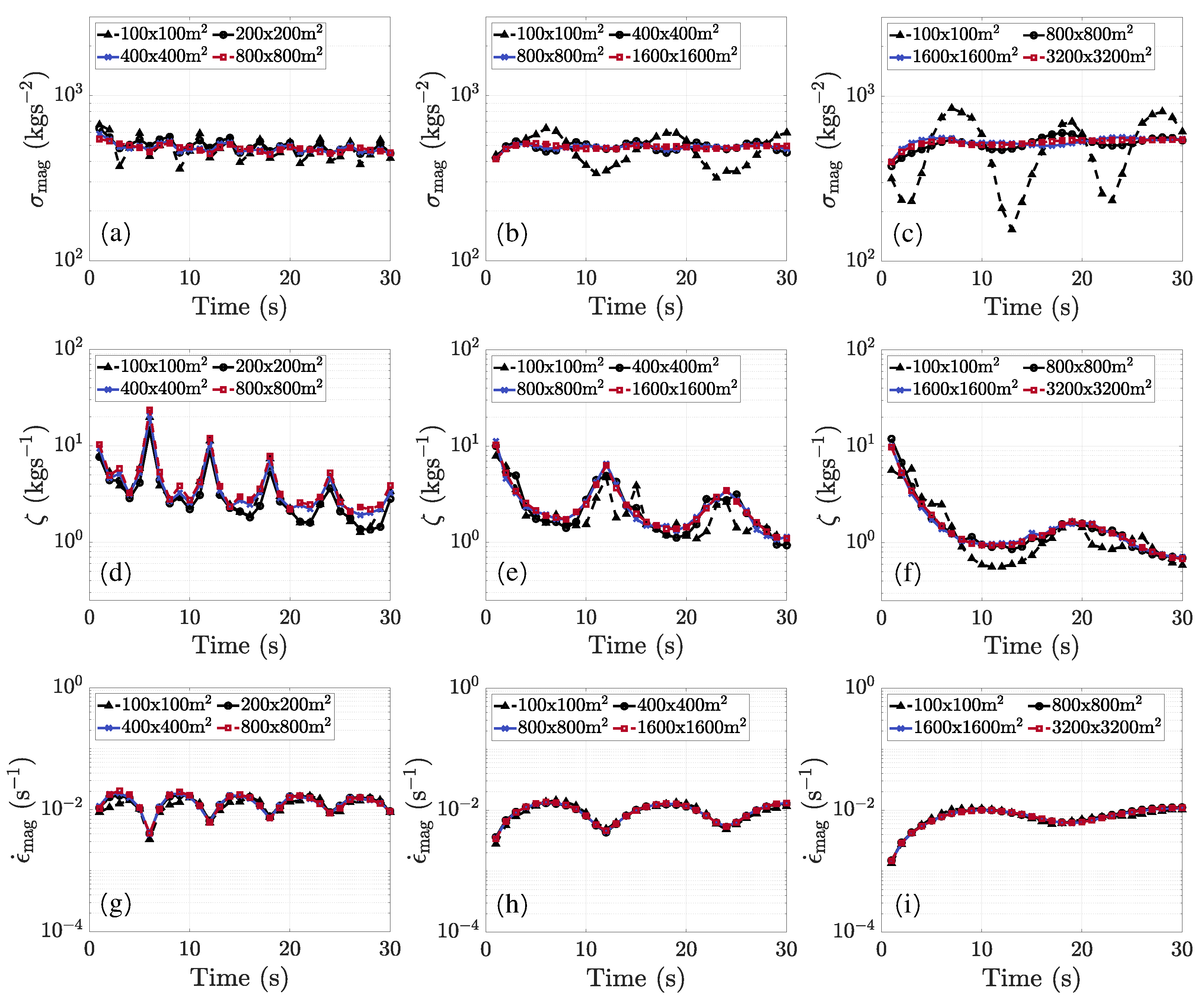
4.2. Domain Size Convergence Analysis

The threshold for convergence with respect to the minimum required domain size is found by calculating the domain-averaged stress and strain magnitudes, σ mag and ϵ ˙ mag , respectively, as well as bulk viscosity, ζ , for increasing inner domain sizes. Once the average is unaffected by changes in the domain size, the transition from small- to large-scale modelling is identified, and the link to a phenomenological model using homogeneous material properties can be established.
A total domain size of 3600 × 3600 m 2 is considered, from which results are extracted for smaller inner domains, ranging from 100 × 100 m 2 to 3200 × 3200 m 2 . This ensures a boundary zone of 400 m around the largest inner domain to exclude unwanted boundary effects due to the zero-gradient boundary conditions. Figure 3 shows the smallest three inner domain sizes ranging from 100 × 100 m 2 to 400 × 400 m 2 .
With 20 m -diameter ice floes the ice floe concentration from the largest inner domain size, 3200 × 3200 m 2 , to the smallest inner domain size, 100 × 100 m 2 , ranges from 40 % to 38 % , due to a randomly distributed sea ice layout.
Figure 4 shows the overall domain-averaged sea ice rheology variables (stress, strain rate and bulk viscosity) in both, ice floes and grease ice, for different domain sizes and three different wave periods. Clearly, smaller wave periods reduce the required domain size for convergence. For the largest wave period of T = 20 s , the threshold is identified at an inner domain size of 1600 × 1600 m 2 , where the blue and red curves in Figure 4c,f,i, which represent an inner domain size of 1600 × 1600 m 2 and 3200 × 3200 m 2 , respectively, converge. In contrast, for the smallest wave periods T = 6 s , the minimum required inner domain size is only 400 × 400 m 2 .

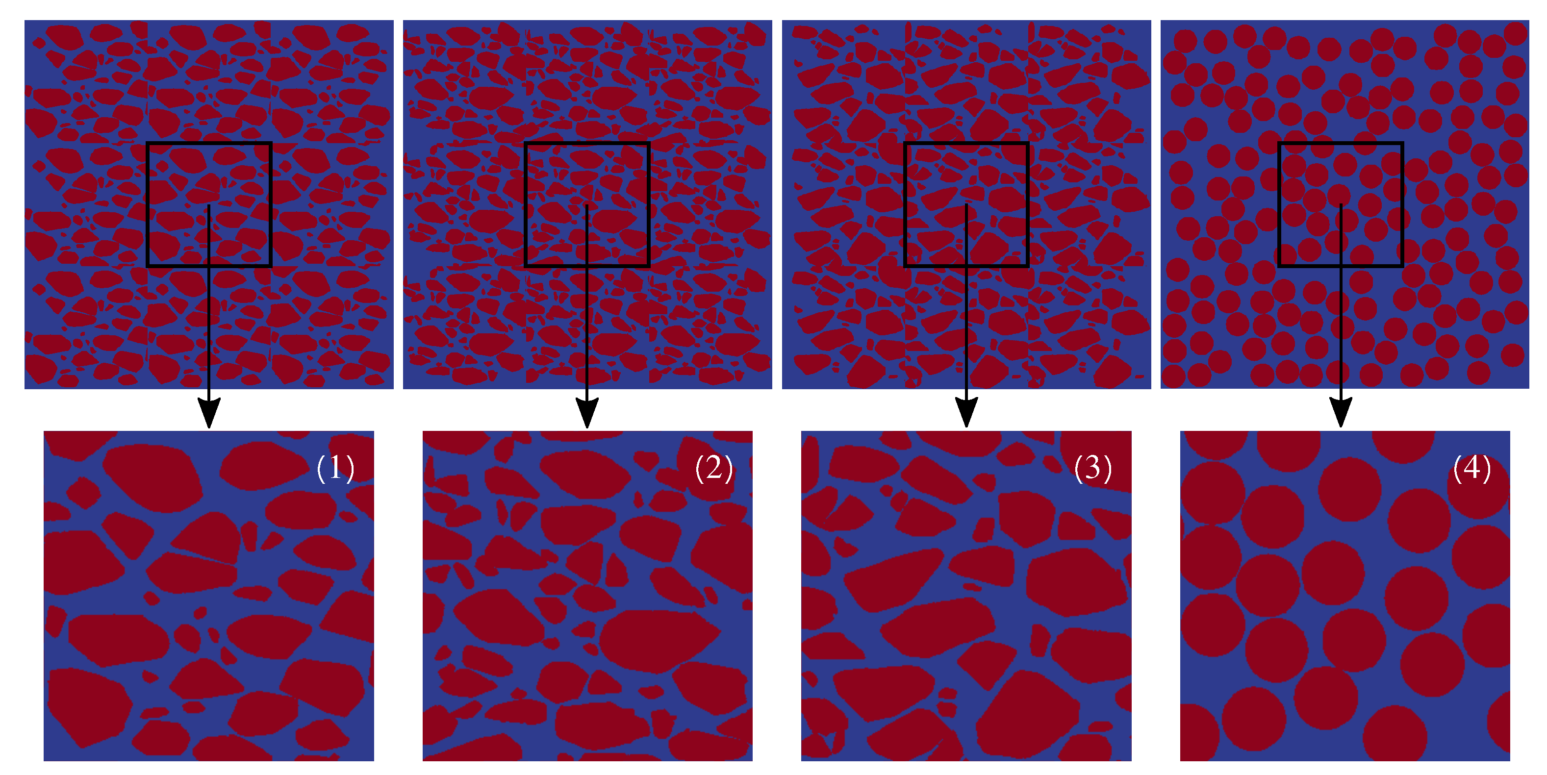
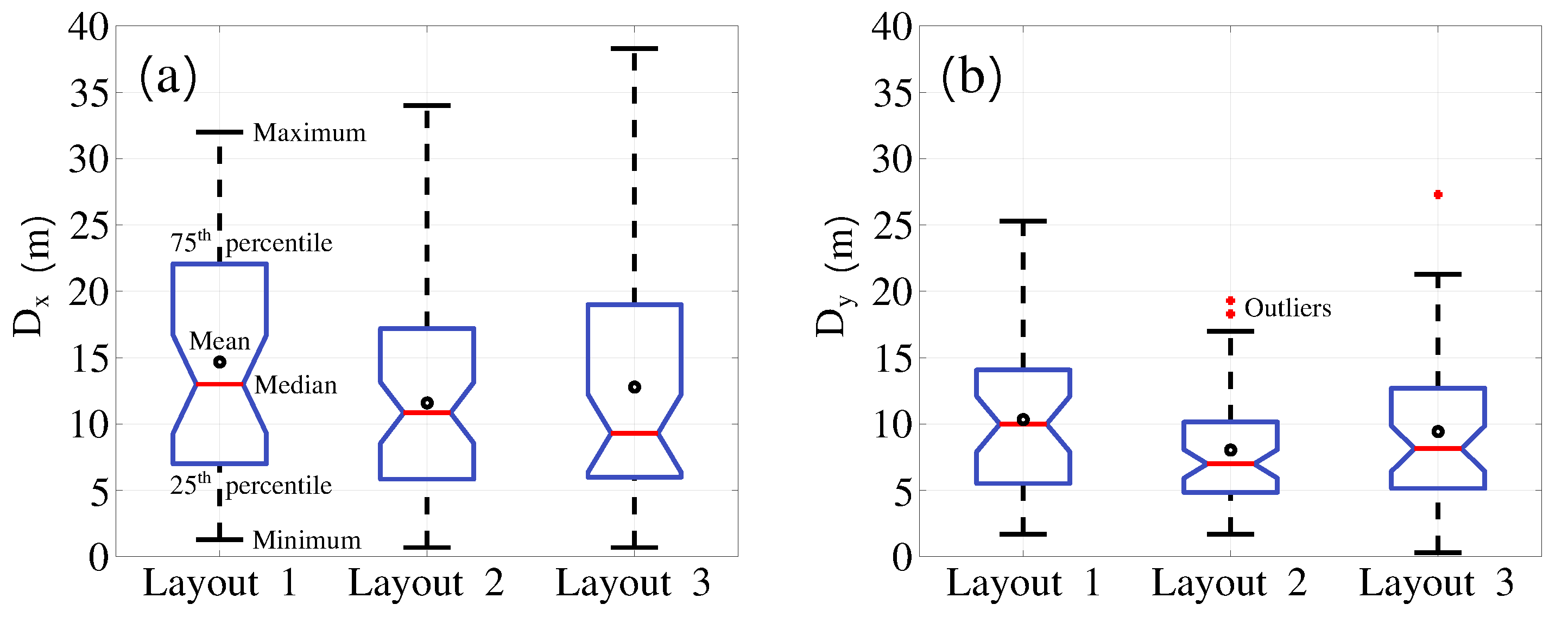
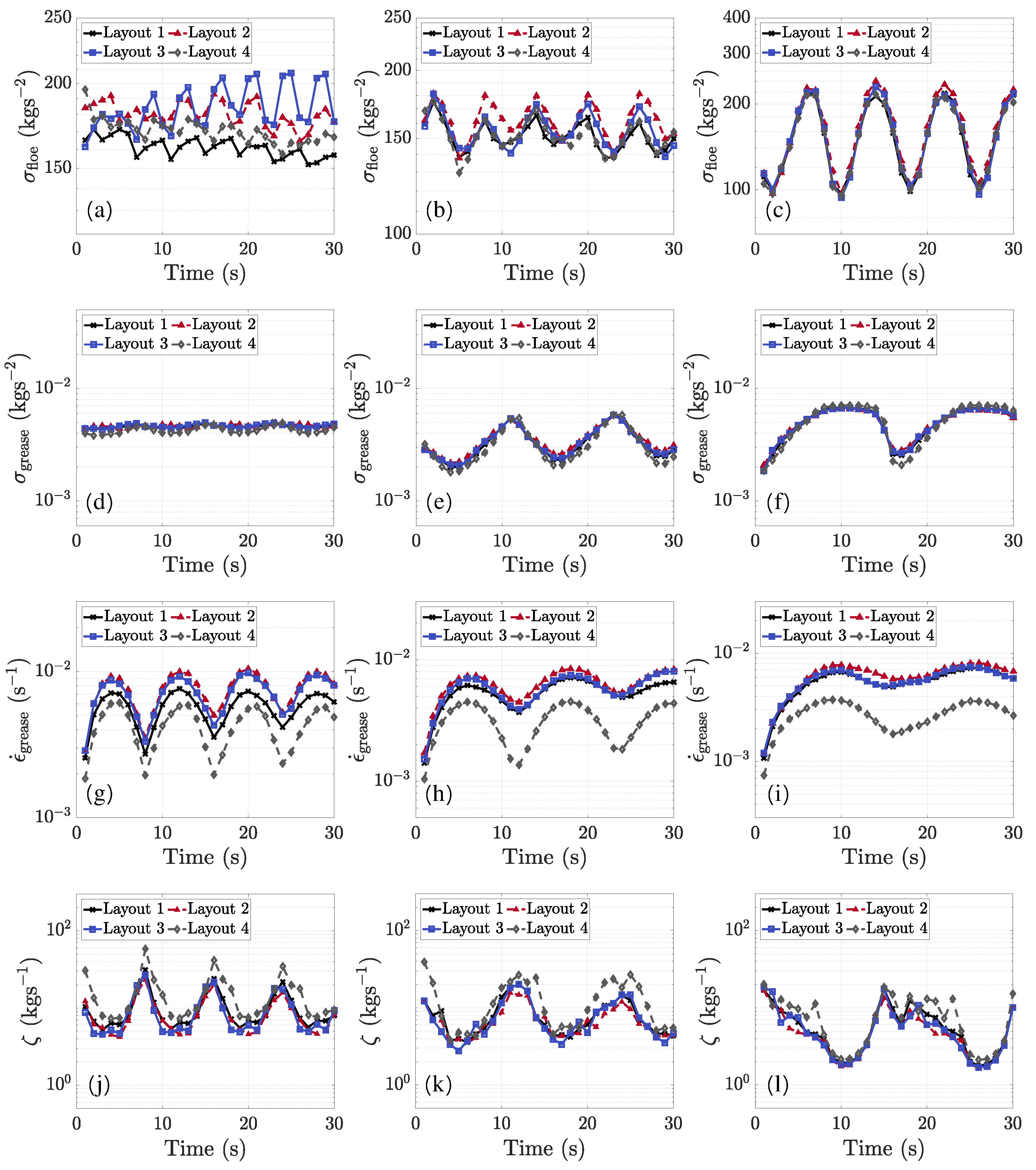
5. Analysis of the Sea Ice Layout and Rheology

In this section the sea ice rheology variables are separately analysed for ice floes and grease ice. Section 4.2 indicates that any inner domain size smaller than 400 × 400 m 2 results in clear differences in mechanical response for any wave period larger than T = 6 s . An inner domain size of 100 × 100 m 2 is therefore expected to produce temporal and spatial fluctuations of the strain rate distribution depending on the ratio of median pancake floe diameter and wavelength, D p , m e d i a n / λ , and thus, warrant detailed small-scale modelling.
Three realistic layouts and one idealised sea ice configuration comparable in terms of sea ice concentration are illustrated in Figure 5. The ice floe caliper diameter ( D x and D y ; in x- and y-direction), standard deviation ( S D x and S D y ; in x- and y-direction), ice floe concentrations, wave characteristics and viscosity are summarised in Table 2 for all four layouts.
Layout differences in ice floe concentration, 57.9 % ( ± 3.2 % ), and median ice floe caliper diameter with 10.8 m ( ± 2.2 m ) in x-direction and 8.7 m ( ± 1.7 m ) in y-direction, respectively, are small. The distribution of the ice floe caliper diameters has been mapped for all realistic sea ice layouts through the use of a boxplot, as shown in Figure 6. Layout 2 has the smallest interquartile range. This is also reflected in the standard deviation, which shows the lowest values in both x- and y-direction for layout 2. This indicates that it features the largest portion of medium-size floes and is the most homogeneous in size. Layout 3, on the other hand, exhibits the largest spread of floe sizes, in particular with regards to large floes.
As layout 2 is the most homogeneous, its mechanical response is expected to be closest to the idealised sea ice layout 4 and is therefore chosen to study the error introduced by completely disregarding floe shape and variations of floe diameter. In order to specifically focus on the sensitivity regarding those two sea ice characteristics and study their effect on stress, strain rate and viscosity variables in both the grease ice and ice floe rheology, the ice floe concentration is chosen to be the same and the mean ice floe caliper diameter in layout 4 has been derived from layout 2, such as that the average area per ice floe, A f l o e = 293 m 2 , is identical.
All sea ice layouts in this analysis are subjected to three different wave forcings via Equation (3) using wave periods ranging between T = 8 and 16 s and for constant wave steepness a k = 0.06 (by varying the wave amplitude). The domain-averaged grease ice viscosity value is ν 0.04 m 2 s 1 in agreement with literature values [1,54,55]. The viscosity of the grease ice rheology, Equation (16), is strain rate-dependent via the ice strength parameter, P, which in turn depends on the empirical constant, P * . The value of P * is chosen such as that the domain-averaged viscosity provides a close match to the predefined value above. For each sea ice layout, three simulations of 30 s are carried out according to the three aforementioned wave periods to elucidate the impact of wave length on the mechanical response.
Figure 7 shows the spatially-averaged stress and strain rate magnitudes in both grease ice and pancake ice floes for wave periods T = 8 s , T = 12 s and T = 16 s with ν 0.04 m 2 s 1 . In Figure 7a–c the spatially-averaged ice floe stress magnitude evolution over time is shown for all sea ice layouts. The average stress in ice floes is similar for all wave periods due to a prescribed wave steepness, a k = 0.06 . An increasing wave period results in an increasing stress amplitude and a decreasing stress frequency. The discrepancy between the stress curves of the four considered layouts increases for a decreasing wave period signifying the mounting influence of the detailed heterogeneous sea dynamics description. Clearly, the realistic sea ice layout 1 exhibits a smaller floe stress magnitude compared to layouts 2 and 3, in particular for the smallest wave period, T = 8 s , as illustrated in Figure 7a. Additionally, it can be observed that the floe stress differences between layouts change with the wave period and that the grease ice stress fluctuations, shown in Figure 7d–f, in particular for T = 8 s , are considerably lower than seen for the floe stress. With regards to influence of floe shape and diameter variations, the floe stress and strain rate response of the idealised sea ice composition (layout 4) is distinctly different from the realistic layout 2, both being underestimated by the idealisation of ice floe geometry. The average discrepancy in the ice floe stress curves between layout 2 and 4 is approximately 7 % .
As mentioned previously, Figure 7d–f show the spatially-averaged grease ice stress for sea ice layouts 1–4. Results of the three realistic sea ice layouts (layout 1–3) are very similar for all wave periods, due to a comparable concentration of grease ice in all layouts. On the other hand, the uniformity of floe diameter and shape results in an average discrepancy in the grease ice stress between layout 2 and the idealised one (layout 4) of about 7 % .
Lastly, Figure 7g–l show the spatially-averaged grease ice strain rate and bulk viscosity for all sea ice layouts. As for the flow stress, the discrepancy between the strain rate evolution in time increases for decreasing wave period looking at the realistic sea ice layouts and a distinctly smaller strain rate magnitude is exhibited for layout 1. Comparing the grease ice strain rate curves of layout 2 and 4, we clearly see that the average strain rate is lower for layout 4, as it was the case for floe and grease ice stress. The average discrepancy in the grease ice strain rate between layout 2 and 4 is substantial with approximately 103 % . From Equation (14) we know that the relation between the grease ice strain rate and viscosity is inversely proportional. An increase in grease ice viscosity results in a decreasing strain rate and vice versa. As these variables are directly related, the average discrepancy in grease ice viscosity between layout 2 and 4 is also quite high, with a value of roughly 42 % .

6. Discussion

From the grid-size analysis performed in Section 4.1, the required cell size providing convergence was determined as 0.33 × 0.33 m 2 . To justify small-scale modelling a domain-size threshold was identified as smaller than 400 × 400 m 2 in Section 4.2 where temporal and spatial fluctuations of the sea ice rheology variables (stress, strain rate and viscosity) become significant for all considered wave periods T = 6–20 s with 20 m -diameter ice floes. This wave period-dependent threshold marks the transition from small- to large-scale modelling where a phenomenological model with homogenised material properties can be utilised.
Simulating three realistic sea ice layouts of 100 × 100 m 2 extracted from in situ images of the Antarctic MIZ, the robustness of the approach has been demonstrated in Section 5. It was found that the mechanical sea ice response tends to become independent of the detailed distribution of floes for wave periods larger than T = 16 s in case of homogeneous sea ice conditions with similar ice concentrations and median floe caliper diameters. This general trend is to be expected, as larger waves cease to directly interact with a single floe and the detail of floe distribution becomes less significant. In contrast, the discrepancy between stress and strain rate curves increases for smaller wave periods and the actual floe geometry needs to be accounted for to accurately capture the mechanical sea ice behaviour. An increasing ratio of ice floe diameter to wavelength results in a reduced stress and strain rate response in the considered realistic sea ice layouts. Based on the observation of significantly larger differences in ice floe stress between layouts compared to that of grease ice, it seems that the Froude–Krylov force is the main source for those observations considering that it solely acts on the ice floe circumference. As such, the dependency on the ratio of floe diameter to wave length becomes significant. It might be also plausible that the relatively large amount of larger floe diameters in layout 1 reduces the wave-floe interaction and thus, floe collision due to larger inertia. Both hypotheses, however, warrant further in-depth investigations.
Lastly, the influence of floe shape and diameter variations was shown to be significant considering additionally an idealised sea ice layout with disk-shaped floes with identical ice concentration and average area per ice floe. The domain-averaged strain rate magnitude and bulk viscosity are mostly affected by the detailed geometrical floe properties, with an average discrepancy of 103 % and 42 % , respectively.

7. Conclusions

In this paper, we presented a new numerical approach to model the small-scale interaction of waves, pancake ice floes and interstitial grease ice. For this, the material behaviour of ice floes and grease ice is separately described considering both characteristic material properties. Ice floes are modelled as elastic solids with high stiffness using generalised Hooke’s law. Grease ice behaves as a viscous fluid obeying a viscous-plastic flow rheology. This two-phase description is in contrast to the commonly used smeared phenomenological approaches in which a large heterogeneous sea ice area is homogenised as one isotropic, continuous material with averaged quantities. To study the influence of wave forcing on the mechanical response of sea ice, a linearised harmonic propagating wave has been imposed on the domain via the Froude–Krylov force emulating the wave pressure field acting on the ice floe circumference and the skin drag acting on the ice basal plane. The form drag on the ice floe due to grease ice is implicitly accounted for by the continuum approach modelling the detailed distribution of both ice constituents throughout the domain.
In summary, results of this paper demonstrate the importance of detailed small-scale modelling on the sub-kilometer scale to resolve the mechanical response of a heterogeneous sea ice cover due to the complex interaction of waves, floes and grease ice. In particular, the floe shape and diameter variations as well as the different wave-ice interaction mechanisms need to be accounted for. The latter comprise the Froude–Krylov force, skin and form drag. Furthermore, the differences in ice rheology need to be considered concerning the solid-like ice floe and the fluid-like grease ice behaviour. Specifically, the influence of the grease viscosity warrants further investigation. If large-scale regional models are to be informed by the actual material behaviour as originated on smaller scale, averaged material parameters need to be obtained from homogenisation and upscaling procedures. These rely on the identification of the minimum domain size threshold where the actual kinematics and material composition of the problem must be addressed in detail and the averaged quantities are statistically representative for larger domains.

Author Contributions

Conceptualisation, R.M.; methodology, R.M. and S.S.; software, R.M. and A.B.; validation, all authors; writing—original draft preparation, R.M.; writing—review and editing, all authors. All authors have read and agreed to the published version of the manuscript.

Funding

This research has been funded by the National Research Foundation of South Africa (Grant Nos. 104839, 105858 and 118745). Opinions expressed and conclusions arrived at are those of the author and are not necessarily to be attributed to the NRF. R.M., S.S. and M.V. acknowledge support from the South African National Antarctic Programme. A.A. and A.T. acknowledge support from the ACE Foundation–Ferring Pharmaceuticals and the Australian Antarctic Science Program (project 4434). AA is supported by the Japanese Society for the Promotion of Science (PE19055).

Institutional Review Board Statement

Not applicable.

Informed Consent Statement

Not applicable.

Data Availability Statement

Not applicable.

Acknowledgments

Computations were performed using facilities provided by the University of Cape Town’s ICTS High Performance Computing team: http://hpc.uct.ac.za accessed on 23 April 2021).

Conflicts of Interest

The authors declare no conflict of interest.

References

  1. Wadhams, P.; Parmiggiani, F.; de Carolis, G. Wave Dispersion by Antarctic Pancake Ice From Sar Images: A Method for Measuring Ice Thickness. Advances in SAR Oceanography from Envisat and ERS Missions. 2006, Volume 613. Available online: https://earth.esa.int/cgi-bin/confseasard75e.html?abstract=110 (accessed on 23 April 2021).
  2. Massom, R.A.; Stammerjohn, S.E. Antarctic sea ice change and variability - Physical and ecological implications. Polar Sci. 2010, 4, 149–186. [Google Scholar] [CrossRef] [Green Version]
  3. Alberello, A.; Bennetts, L.; Heil, P.; Eayrs, C.; Vichi, M.; MacHutchon, K.; Onorato, M.; Toffoli, A. Drift of pancake ice floes in the winter Antarctic marginal ice zone during polar cyclones. J. Geophys. Res. Ocean. 2020, 125, e2019JC015418. [Google Scholar] [CrossRef] [Green Version]
  4. Vichi, M.; Eayrs, C.; Alberello, A.; Bekker, A.; Bennetts, L.; Holland, D.; de Jong, E.; Joubert, W.; MacHutchon, K.; Messori, G.; et al. Effects of an explosive polar cyclone crossing the Antarctic marginal ice zone. Geophys. Res. Lett. 2019, 46, 5948–5958. [Google Scholar] [CrossRef] [Green Version]
  5. Häkkinen, S. A constitutive law for sea ice and some applications. Math. Model. 1987, 9, 81–90. [Google Scholar] [CrossRef] [Green Version]
  6. Hibler, W., III. A dynamic thermodynamic sea ice model. J. Phys. Oceanogr. 1979, 9, 815–846. [Google Scholar] [CrossRef] [Green Version]
  7. Keller, J.B. Gravity waves on ice-covered water. J. Geophys. Res. Ocean. 1998, 103, 7663–7669. [Google Scholar] [CrossRef]
  8. Wang, R.; Shen, H.H. Gravity waves propagating into an ice-covered ocean: A viscoelastic model. J. Geophys. Res. Ocean. 2010, 115, 1–12. [Google Scholar] [CrossRef]
  9. Pritchard, R.S. Mathematical characteristics of sea ice dynamics models. J. Geophys. Res. Ocean. 1988, 93, 15609–15618. [Google Scholar] [CrossRef]
  10. Kleine, E.; Sklyar, S. Mathematical features of Hibler’s model of large-scale sea-ice dynamics. Dtsch. Hydrogr. Z. 1995, 47, 179–230. [Google Scholar] [CrossRef]
  11. Rampal, P.; Weiss, J.; Marsan, D.; Lindsay, R.; Stern, H. Scaling properties of sea ice deformation from buoy dispersion analysis. J. Geophys. Res. Ocean. 2008, 113. [Google Scholar] [CrossRef] [Green Version]
  12. Dansereau, V.; Weiss, J.; Saramito, P.; Lattes, P. A Maxwell elasto-brittle rheology for sea ice modelling. Cryosphere 2016, 10, 1339–1359. [Google Scholar] [CrossRef] [Green Version]
  13. Mehlmann, C.; Richter, T. A finite element multigrid-framework to solve the sea ice momentum equation. J. Comput. Phys. 2017, 348, 847–861. [Google Scholar] [CrossRef]
  14. Mehlmann, C.; Richter, T. A modified global Newton solver for viscous-plastic sea ice models. Ocean Model. 2017, 116, 96–107. [Google Scholar] [CrossRef]
  15. Biddle, L.; Swart, S. The observed seasonal cycle of submesoscale processes in the Antarctic marginal ice zone. J. Geophys. Res. Ocean. 2020, 125, e2019JC015587. [Google Scholar] [CrossRef]
  16. Leppäranta, M. The Drift of Sea Ice; Springer Science & Business Media: Berlin/Heidelberg, Germany, 2011. [Google Scholar]
  17. Shen, H.; Perrie, W.; Hu, Y.; He, Y. Remote sensing of waves propagating in the marginal ice zone by SAR. J. Geophys. Res. Ocean. 2018, 123, 189–200. [Google Scholar] [CrossRef]
  18. Alberello, A.; Bennetts, L.; Onorato, M.; Vichi, M.; MacHutchon, K.; Eayrs, C.; Ntamba, B.N.; Benetazzo, A.; Bergamasco, F.; Nelli, F.; et al. An extreme wave field in the winter Antarctic marginal ice zone during an explosive polar cyclone. arXiv 2021, arXiv:2103.08864. [Google Scholar]
  19. Toyota, T.; Kohout, A.; Fraser, A.D. Formation processes of sea ice floe size distribution in the interior pack and its relationship to the marginal ice zone off East Antarctica. Deep Sea Res. Part II Top. Stud. Oceanogr. 2016, 131, 28–40. [Google Scholar] [CrossRef] [Green Version]
  20. Squire, V.A. Of ocean waves and sea-ice revisited. Cold Reg. Sci. Technol. 2007, 49, 110–133. [Google Scholar] [CrossRef]
  21. Shen, H.H.; Hibler, W.D., III; Leppäranta, M. The role of floe collisions in sea ice rheology. J. Geophys. Res. Ocean. 1987, 92, 7085–7096. [Google Scholar] [CrossRef]
  22. Alberello, A.; Onorato, M.; Bennetts, L.; Vichi, M.; Eayrs, C.; MacHutchon, K.; Toffoli, A. Brief communication: Pancake ice floe size distribution during the winter expansion of the Antarctic marginal ice zone. Cryosphere 2019, 13, 41–48. [Google Scholar] [CrossRef] [Green Version]
  23. Alberello, A.; Nelli, F.; Dolatshah, A.; Bennetts, L.G.; Onorato, M.; Toffoli, A. An Experimental Model of Wave Attenuation in Pancake Ice. In Proceedings of the 29th International Ocean and Polar Engineering Conference, International Society of Offshore and Polar Engineers, Honolulu, HI, USA, 16–21 June 2019. [Google Scholar]
  24. Kohout, A.; Williams, M.; Dean, S.; Meylan, M. Storm-induced sea-ice breakup and the implications for ice extent. Nature 2014, 509, 604–607. [Google Scholar] [CrossRef]
  25. Stopa, J.E.; Sutherland, P.; Ardhuin, F. Strong and highly variable push of ocean waves on Southern Ocean sea ice. Proc. Natl. Acad. Sci. USA 2018, 115, 5861–5865. [Google Scholar] [CrossRef] [Green Version]
  26. Hopkins, M.A. On the mesoscale interaction of lead ice and floes. J. Geophys. Res. Ocean. 1996, 101, 18315–18326. [Google Scholar] [CrossRef]
  27. Herman, A. Discrete-Element bonded-particle Sea Ice model DESIgn, version 1.3a—Model description and implementation. Geosci. Model. Dev. 2016, 9, 1219–1241. [Google Scholar] [CrossRef] [Green Version]
  28. Herman, A. Numerical modeling of force and contact networks in fragmented sea ice. Ann. Glaciol. 2013, 54, 114–120. [Google Scholar] [CrossRef] [Green Version]
  29. Herman, A.; Cheng, S.; Shen, H.H. Wave energy attenuation in fields of colliding ice floes–Part 2: A laboratory case study. Cryosphere 2019, 13, 2901–2914. [Google Scholar] [CrossRef] [Green Version]
  30. Bennetts, L.G.; Alberello, A.; Meylan, M.H.; Cavaliere, C.; Babanin, A.V.; Toffoli, A. An idealised experimental model of ocean surface wave transmission by an ice floe. Ocean Model. 2015, 96, 85–92. [Google Scholar] [CrossRef] [Green Version]
  31. Skene, D.; Bennetts, L.; Meylan, M.; Toffoli, A. Modelling water wave overwash of a thin floating plate. J. Fluid Mech. 2015, 777. [Google Scholar] [CrossRef] [Green Version]
  32. Nelli, F.; Bennetts, L.G.; Skene, D.M.; Toffoli, A. Water wave transmission and energy dissipation by a floating plate in the presence of overwash. J. Fluid Mech. 2020, 889. [Google Scholar] [CrossRef]
  33. Damsgaard, A.; Adcroft, A.; Sergienko, O. Application of discrete element methods to approximate sea ice dynamics. J. Adv. Model. Earth Syst. 2018, 10, 2228–2244. [Google Scholar] [CrossRef]
  34. Rabatel, M.; Labbé, S.; Weiss, J. Dynamics of an assembly of rigid ice floes. J. Geophys. Res. Ocean. 2015, 120, 5887–5909. [Google Scholar] [CrossRef] [Green Version]
  35. McNamara, S. Molecular dynamics method. Discrete Numer. Model. Granul. Mater. 2011. [Google Scholar] [CrossRef]
  36. Holthuijsen, L.H. Waves in Oceanic and Coastal Waters; Cambridge University Press: Cambridge, UK, 2010. [Google Scholar]
  37. Herman, A. Wave-Induced Surge Motion and Collisions of Sea Ice Floes: Finite-Floe-Size Effects. J. Geophys. Res. Ocean. 2018, 123, 7472–7494. [Google Scholar] [CrossRef]
  38. Thorndike, A.S.; Rothrock, D.A.; Maykut, G.A.; Colony, R. The Thickness Distribution of Sea Ice. J. Geophys. Res. 1975, 80, 4501. [Google Scholar] [CrossRef]
  39. Leppäranta, M.; Hibler, W.D. The role of plastic ice interaction in marginal ice zone dynamics. J. Geophys. Res. 1985, 90, 11899. [Google Scholar] [CrossRef]
  40. Hunke, E.C.; Dukowicz, J.K. An Elastic—Viscous—Plastic Model for Sea Ice Dynamics. J. Phys. Ocean. 1997, 27, 1849–1867. [Google Scholar] [CrossRef] [Green Version]
  41. Ferziger, J.H.; Peric, M. Computational Methods for Fluid Dynamics; Springer: Berlin, Germany, 2002; p. 423. [Google Scholar] [CrossRef] [Green Version]
  42. Roenby, J.; Bredmose, H.; Jasak, H. A computational method for sharp interface advection. R. Soc. Open Sci. 2016, 3, 160405. [Google Scholar] [CrossRef] [Green Version]
  43. Roenby, J.; Bredmose, H.; Jasak, H. IsoAdvector: Geometric VOF on general meshes. In OpenFOAM®; Springer: Berlin, Germany, 2019; pp. 281–296. [Google Scholar]
  44. Steiner, N. Introduction of variable drag coefficients into sea-ice models. Ann. Glaciol. 2001, 33, 181–186. [Google Scholar] [CrossRef] [Green Version]
  45. Shapiro, L.H.; Johnson, J.B.; Sturm, M.; Blaisdell, G.L. Snow Mechanics: Review of the State of Knowledge and Applications; Technical Report; Cold Regions Research and Engineering Laboratory: Hanover, South Africa, 1997. [Google Scholar]
  46. Worby, A.P.; Geiger, C.A.; Paget, M.J.; Van Woert, M.L.; Ackley, S.F.; DeLiberty, T.L. Thickness distribution of Antarctic sea ice. J. Geophys. Res. Ocean. 2008, 113. [Google Scholar] [CrossRef] [Green Version]
  47. McGuinness, M.; Williams, M.; Langhorne, P.; Purdie, C.; Crook, J. Frazil deposition under growing sea ice. J. Geophys. Res. Ocean. 2009, 114. [Google Scholar] [CrossRef] [Green Version]
  48. Radia, N.V. Frazil Ice Formation in the Polar Oceans. Ph.D. Thesis, University College London, London, UK, 2014. [Google Scholar]
  49. Schulkes, R.; Morland, L.; Staroszczyk, R. A finite-element treatment of sea ice dynamics for different ice rheologies. Int. J. Numer. Anal. Methods Geomech. 1998, 22, 153–174. [Google Scholar] [CrossRef]
  50. Lu, P.; Li, Z.; Cheng, B.; Leppäranta, M. A parameterization of the ice-ocean drag coefficient. J. Geophys. Res. Ocean. 2011, 116. [Google Scholar] [CrossRef]
  51. Andreas, E.L.; Tucker, W.B., III; Ackley, S.F. Atmospheric boundary-layer modification, drag coefficient, and surface heat flux in the Antarctic marginal ice zone. J. Geophys. Res. Ocean. 1984, 89, 649–661. [Google Scholar] [CrossRef]
  52. Hibler, W.D. A Viscous Sea Ice Law as a Stochastic Average of Plasticity. J. Geophys. Res. 1979, 82, 206–209. [Google Scholar] [CrossRef]
  53. Alberello, A.; Nelli, F.; Dolatshah, A.; Bennetts, L.G.; Onorato, M.; Toffoli, A. A Physical Model of Wave Attenuation in Pancake Ice. Int. J. Offshore Polar Eng. 2021. [Google Scholar]
  54. Newyear, K.; Martin, S. Comparison of laboratory data with a viscous two-layer model of wave propagation in grease ice. J. Geophys. Res. Ocean. 1999, 104, 7837–7840. [Google Scholar] [CrossRef]
  55. Wang, R.; Shen, H.H. Cold Regions Science and Technology Experimental study on surface wave propagating through a grease—pancake ice mixture. Cold Reg. Sci. Technol. 2010, 61, 90–96. [Google Scholar] [CrossRef]
Figure 1. Three different grid refinement levels of a 300 × 300 m 2 -outer domain of randomly distributed disk-shaped 20 m -diameter pancake floes each with 100 × 100 m 2 -inner domains of following discretisations: (a) 2500 cells with a 2 × 2 m 2 cell size, (b) 10,000 cells with a 1 × 1 m 2 cell size and (c) 160,000 cells with a 0.25 × 0.25 m 2 cell size. Red and blue represent ice floes and grease ice, respectively. The numerical interface is indicated by the white colour.
Fluids 06 00176 g001
Figure 2. Comparison of the spatial average of the main sea ice rheology variables for four different discretisation sizes: (a) stress magnitude, (b) bulk viscosity and (c) strain rate magnitude.
Fluids 06 00176 g002
Figure 3. Inner domain sizes ranging from 100 × 100 m 2 to 400 × 400 m 2 with varying ice floe concentration. Ice floes are modelled as disk-shaped floes of 20 m -diameter. Red and blue represent ice floes and grease ice, respectively.
Fluids 06 00176 g003
Figure 4. Comparing the domain-averaged sea ice rheology variables for different inner domain sizes and three different wave periods. Stress magnitude for (a) T = 6 s , (b) T = 12 s and (c) T = 20 s . Bulk viscosity for (d) T = 6 s , (e) T = 12 s and (f) T = 20 s . Strain rate magnitude for (g) T = 6 s , (h) T = 12 s and (i) T = 20 s .
Fluids 06 00176 g004
Figure 5. Three realistic sea ice layouts (1–3) and one idealised with disk-shaped floes (4), each with a 100 × 100 m 2 inner domain embedded in a 300 × 300 m 2 outer domain.
Fluids 06 00176 g005
Figure 6. Boxplots for all three realistic sea ice layouts, showing the distribution of the (a) caliper diameter in x-direction and (b) caliper diameter in y-direction.
Fluids 06 00176 g006
Figure 7. Spatially-averaged mechanical sea ice response for layouts 1–4 with ν 0.04 m 2 s 1 showing ice floe stress for (a) T = 8 s , (b) T = 12 s and (c) T = 16 s . Grease ice stress for (d) T = 8 s , (e) T = 12 s and (f) T = 16 s . Grease ice strain rate for (g) T = 8 s , (h) T = 12 s and (i) T = 16 s . Bulk viscosity for (j) T = 8 s , (k) T = 12 s and (l) T = 16 s .
Fluids 06 00176 g007
Table 2. Parameters used in the analysis of sea ice composition and rheology, where XCD and YCD denote the ice floe caliper diameter in x- and y-directions, respectively. The standard deviation in x- and y-directions is indicated by XSD and YSD, respectively.
ParameterDefinitionValueUnit
D x , m e d i a n median XCD layout 1, 2, 3, 413.0, 11.0, 9.3, 9.7m
D y , m e d i a n median YCD layout 1, 2, 3, 410.0, 7.0, 8.0, 9.7m
S D x XSD layout 1, 2, 3, 48.8, 7.3, 9.2, 0m
S D y YSD layout 1, 2, 3, 45.5, 4.3, 5.6, 0m
Aice floe concentration layout 1, 2, 3, 454.7, 59.7, 57.3, 59.7%
Twave period8, 12, 16s
awave amplitude1, 2.1, 3.8m
λ wavelength100, 225, 400m
ν grease ice viscosity0.04 m 2 s 1
P * grease ice strength0.024 N m 3
Publisher’s Note: MDPI stays neutral with regard to jurisdictional claims in published maps and institutional affiliations.

