The Emergence and Identification of Large-Scale Coherent Structures in Free Convective Flows of the Rayleigh-Bénard Type

Abstract

The revealing of the turbulence archetypes is one of the fundamental problems in the study of turbulence, which is important not only from the fundamental point of view but also for practical applications, e.g., in geophysics of ocean and lakes. The paper is devoted to the study of the emergence of coherent structures and the identification of their turbulent archetypes, typical for the free convective flows of the Rayleigh-Bénard type. Using Direct Numerical Simulation, we perform a numerical study of two refined convective flows: convection in a cylinder heated from below and internally heated convection in a layer. The main purpose of the study is identifying coherent structures (CS), investigating its main features and properties, and determining the turbulence archetypes using the anisotropy invariant map (AIM). We show that, in both configurations considered, CS takes place. In a cylinder, CS is a single large-scale vortex that can rotate azimuthally in non-titled container, but is almost “fixed” in the case of slightly tilted cylinder; in a layer, CS is a quasi-2D vortex, which can arise, exist for some time, disrupt, and then re-emerge again in the orthogonal direction. Nevertheless, the turbulence archetypes represented by the AIM are quite similar for both cases, and there are the distinct CS fingerprints on AIM.

1. Introduction

Usually the studies of turbulent transfer processes in natural geophysical flows are complicated due to the variety of energy forcing. For example, the turbulence production in the surface layers of ocean and lake water bodies may be the result of wind, waves, heating/cooling, tides, seiches, or geostrophical circulations. Therefore the structure of turbulence generated by mean velocity gradient (wind stress), wave-shear interaction (like in the case of Langmuir circulation), or gravitational instability (during night cooling or under-ice inhomogeneous heating of the water column) depends crucially on the type of the forcing. In this regard one can even distinguish between the different “archetypes” of turbulence [1].

The revealing of these archetypes is one of the fundamental problems of turbulence. On the other hand, the thorough description of the archetypes is of great practical importance, considering the variety of water bodies’ responses to external forcing of different nature. In particular, most processes and values of interest (like temperature profile evolution, mixing intensity, thermocline dynamics, etc.) result from simultaneous multiple forcings. Thus to achieve the proper forecasting of system response, the splitting criteria for deriving the contribution of each type of forcing is necessary.

Each turbulence archetype demonstrates the inherent patterns of turbulence parameters spatial distribution and specific features of their temporal evolution. As for these parameters, not only turbulence intensities ⟨u_i′²⟩ (u_i′—pulsation of the velocity along i-th axis; angular brackets mean the averaging in time), but also the anisotropy characteristics like the so-called anisotropy tensor [2,3] a_ij = ⟨u_i′u_j′⟩/(2k)—δ_ij/3 (here k is the turbulence kinetic energy) are of primary interest. The latter ones, in particular, describe the inter-component energy transfer and, supposedly, govern the specifics of mixing processes over a wide range of scales. In this connection, it is worthy to note, that the problem of mixing efficiency η estimation remains still challenging. These estimations for stratified turbulence, reported in a large number of papers, vary from a few percent [4] to 65% [5], though the widely accepted value is 17% (see [6] for example). It cannot be ruled out that just the turbulence archetype variability leads to the crucial differences in estimating the mixing efficiency.

The powerful tool for studying turbulence anisotropy properties is based on the analysis of the second II = a_ija_ji/2 (summation on repeated indexes henceforward) and third III = a_ija_jla_li/3 invariants of the anisotropy tensor. For any given values of invariants II and III, one may represent each state of turbulence by the point on the Anisotropy Invariant Map (AIM) [7,8,9,10,11]. Physically acceptable values are restricted by the realizability requirements (positive definiteness of the turbulent stresses matrix). The correspondent domain on II–III plane is usually referred to as the Lumley triangle (Figure 1). The upper bound of this domain (the segment AB of the line II = 1/9+3III in Figure 1) corresponds to the so called 2D turbulence, the lateral sides AC and BC present the axisymmetric turbulence states II = 3(III/2)^2/3 with one (AC, ”rod-like” pulsations) or two (BC, “disk-like” pulsations) components dominating [9]. Isotropic turbulence is presented by point C with coordinates (0, 0). In addition to the classic triangle, some alternative versions of AIM are widely used, in particular, by substituting coordinates II and III by ζ = (III /2)^1/3 and η = (II/3)^1/2 (see [3] for more details and wider examples).

Each turbulence archetype can be visualized by mapping the turbulent states along vertical or horizontal lines (if all six turbulent stresses are measured or calculated). The correspondent “trajectories” on AIM one can be regarded as the unique “portrait” or fingerprint of the archetype. The gallery of such portraits, based on experimental data or computer simulations, is widely presented in literature for both geophysical [2] and technological [12,13] flows. Even though the high degree of anisotropy is the common feature of most geophysical flows, the details of AIM trajectories differ sufficiently, illustrating the complicated interplay between “rod-like” and “disk-like”, 2D turbulent structures. The comparative analysis of these trajectories was carried out for Langmuir circulation dominated and convective flows [14], channel flows and mixing layers, wind driven and tidal flows [2]. The unsteady flows also demonstrate the unique AIM trajectories, as in the case of breaking Kelvin-Helmholtz wave train [15].

In some cases, the special details of AIM trajectories are viewed as indirect indicator of the large-scale quasi-deterministic vortex (coherent structures, CS) presence. In particular, for the case of Rayleigh-Bénard convection, trajectories, which are pressed against “rod-like” turbulence limiting curve, might indicate the presence of two-dimensional convection rolls [16]. The similar pressing in rotating flows may serve as a marker of columnar vortex plumes development [10]. On the contrary, the inverse trend—trajectory transformation from right-hand AIM boundary aligning to ‘C-shaped’ form, observed for turbulent Couette channel flow—may be treated as the result of Langmuir forcing and the onset of Langmuir supercells [1,14].

A related issue, which is being intensively investigated, is flow reversals, i.e., change in flow direction inside CS due to its rotation or cessation [17,18,19]. In particular, using Direct Numerical Simulation, authors of [18] showed that flow reversal in a Rayleigh-Bénard convection in a cylinder occurs by two kinds of reorientations: rotation-led and cessation-led. The cessation of CS followed by a restart in a random direction, and sometimes double cessation can occur. The unsteady AIM analysis (i.e., temporal variability of AIM trajectories) can reveal some important aspects of the flow reversals, in particular, the change in turbulence archetype due to CS cessation and re-starting.

In general, the revealing of relationships between CS and AIM images of turbulent structures remains the challenging issue, in both fundamental and practical dimensions. As for applied aspects, this issue is of prior interest for problems such as dynamics and spatial distribution of non-motile plankton populations [20,21,22] and sediment resuspension [14].

Only a few attempts of AIM-based CS identification and quantitative description is presented in the literature [23]; as a whole, the problem looks underdeveloped.

This paper is devoted to the study of turbulent archetypes, typical for heat-induced forcing, which triggers gravitational instability and Rayleigh-Bénard type convection. The flows driven by buoyancy are ubiquitous in geophysics, astrophysics, and technological applications. In a number of cases such flows occur in a shear-free environment, so the problem of archetype identification is sufficiently simplified. On the other hand, the AIM analysis for this type of flow is often restricted because of the lack of directly available experimental data (like in the cases of convection in Earth’s mantle and stars or penetrative convection in ice-covered lakes [24]). In this regard, computational methods, including Large Eddy Simulation (LES) and Direct Numerical Simulations (DNS), are in special demand.

In this article we present the results of DNS computations for two refined convective flows of the Rayleigh-Bénard type (detailed overview of this topic can be found, for example, in papers [25,26]). The first considered problem is the Rayleigh-Bénard convection in a cylinder. It should be noted that there is a large number of both experimental [27,28,29,30] and numerical [31,32,33] studies of fluid convection in cylindrical containers with different ratios of the container diameter D to its height H (Γ = D/H) in a wide range of Prandtl numbers. Of the cited papers, a number of publications consider the case of Γ = 1 [27,28,32]. A characteristic feature of the flow here is the presence of large coherent vortex structure that form the so-called large-scale circulation. In the case of a container with Γ = 1, the large-scale coherent structure is a single vortex. One of the features in such flow is the random oscillations of the vortex in the azimuthal direction. These displacements of the large-scale circulation in the azimuthal direction lead to flow reversals and vastly complicate the process of obtaining statistical data on the three-dimensional structure, as well as the local characteristics of turbulent transport. The situation is improved if some stabilizing external factor is artificially introduced, by means of which the large-scale circulation is “fixed” in a certain azimuthal position. For example, in a number of experimental [28,34,35,36] and numerical [37,38,39] works, it was shown that the tilt of the container by a small angle almost completely “fixes” the CS in a certain position. In the paper, we show the results of our numerical simulation of the Rayleigh-Bénard convection in a cylinder, both tilted and non-tiled, and perform the AIM analysis of the large-scale coherent structure.

The second case considered is the convection of an internally heated fluid. Such problem definition differs from the more studied phenomenon of Rayleigh–Bénard convection where motion is driven by thermal conditions at the fluid boundaries. However, the main features of the flow remain very similar [40]. It should be noted that there are many works devoted to classic Rayleigh–Bénard convection, where the emergence and the features of the large-scale coherent structures have been actively studied [41,42,43,44,45]. For example, in [45] such large-scale structures are investigated by analyzing the turbulent kinetic energy and the thermal variance spectra. Another method, which is widely used for CS identification in Rayleigh–Bénard convection, is the flow mode decomposition analysis using Fourier mode decomposition or proper orthogonal decomposition (POD) [46,47,48,49,50], where the instantaneous flow field is projected onto orthogonal basis, and the amplitude of the flow mode takes on the role of a measure of each flow mode strength. Such methods are very robust in case when the possible modes can be known in advance. On the other hand, flow mode decomposition method requires data in the entire geometric domain, which makes it impossible to use it as a tool for identifying CS in experimental observations. The studies of the large-scale coherent structures in internally heated fluid are mostly devoted to the analysis of the mean properties and the turbulence characteristics [40,51,52,53,54,55].

The analysis of large-scale CS, both in an internally heated layer and in a cylindrical container, is quite difficult due to the presence of uncontrolled low-frequency azimuthal oscillations (in case of cylinder) or to the possibility of sudden destruction of CS and subsequent appearance with a different orientation (in case of layer). Such low-frequency changes in the orientation of CS can be reflected in the distribution of AIM trajectories in a rather complicated way and require a separate study. In this paper, we restrict ourselves to studying “fixed” structures, i.e., structures that keep their averaged position in space for a sufficiently long period of time.

Thereby, the revealing of “fixed” CS and AIM trajectories are the focus of the study. Note that the chosen flows differ sufficiently with regard to boundary conditions and the type of forcing. Research questions included, in particular, the following topics:

• Are the flows self-organized (in the sense of CS presence) or constitute the sequence of irregular “thermals”?
• If CS are present, what factors govern their stability and temporal variability?
• Are the turbulence archetypes similar for two chosen types of forcing?
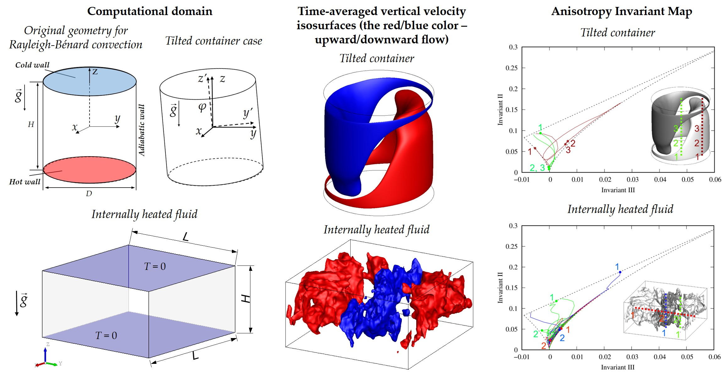
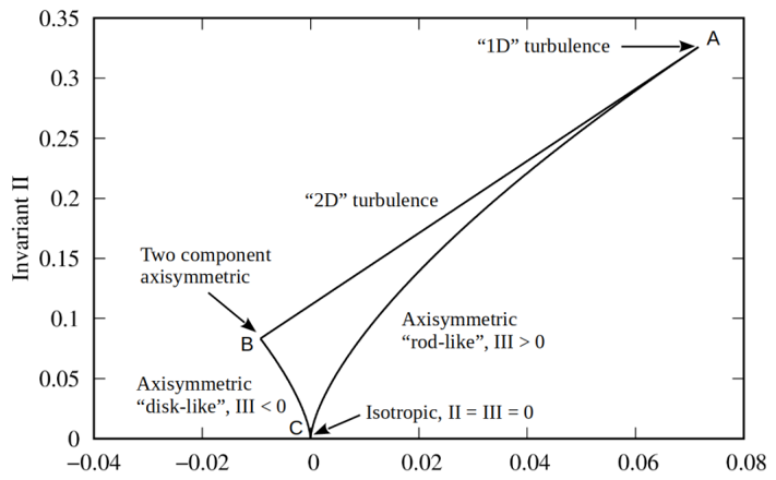
• What are the CS fingerprints (if any) on AIM?

The two last questions mentioned are the main topic of the paper. Our main idea is that a large-scale CS can be identified by analyzing the corresponding AIM along different spatial lines. This is of special interest in experimental study, where often only limited flow data can be obtained. In the paper, using numerical analysis, we try to identify main features of the Rayleigh-Bénard convection associated with CS. We argue that AIM analysis can help identify the CS. This goal is achieved by numerically investigating two relatively different problems of Rayleigh-Bénard convection. Thus, the paper is structured as follows: in Section 2, we present two problem definitions, first is the Rayleigh-Bénard convection in a cylinder, where there is only one distinguishable CS, and the second is internally heated convection in a layer, where emergence and behavior of CS is insufficiently studied in literature. In Section 3, we firstly present the results, obtained for the convection in a cylinder, and perform the analysis of the AIM for this case. Secondly, we present results of numerical simulation of internally heated convection and perform the analysis of emergence and behavior of the CS there. Section 4 is devoted to analysis of the common features of the considered flows, including comparing of the AIM, obtained for two cases. The last section, Summary, contains main considerations obtained in the paper.

2. Problem Definition, Mathematical Model and Numerical Aspects

We consider two cases of the turbulent convection of Rayleigh-Bénard type where large-scale coherent structures arise: convection in a cylinder heated from below and internally heated with constant volumetric heat source.

Turbulent heat and mass transfer in both cases are described by Navier-Stokes equations for incompressible fluid using Boussinesq approximation for buoyancy force coupled with energy equation for incompressible fluid:

$$\nabla \cdot \overrightarrow{V}=0$$

$$\frac{\partial \overrightarrow{V}}{\partial t}+\left(\overrightarrow{V}\cdot \nabla \right)\overrightarrow{V}=-\frac{1}{\rho }\nabla p+\beta \left(T_0-T\right)\overrightarrow{g}+\nu {\nabla }^2\overrightarrow{V}$$

$$\frac{\partial T}{\partial t}+\left(\overrightarrow{V}\cdot \nabla \right)T=a{\nabla }^{2}T+Q$$

where $\overrightarrow{V}=\left(V_x,V_y,V_z\right)$ is the velocity field; t is the time, p is the pressure, T is the temperature, ρ is the medium density, a is the thermal diffusivity coefficient, ν is the kinematic viscosity, β is the thermal expansion coefficient, $\overrightarrow{g}$ is the gravitational acceleration, T₀ is the temperature under hydrostatic equilibrium, Q is the volumetric heat source in case of internally heated convection.

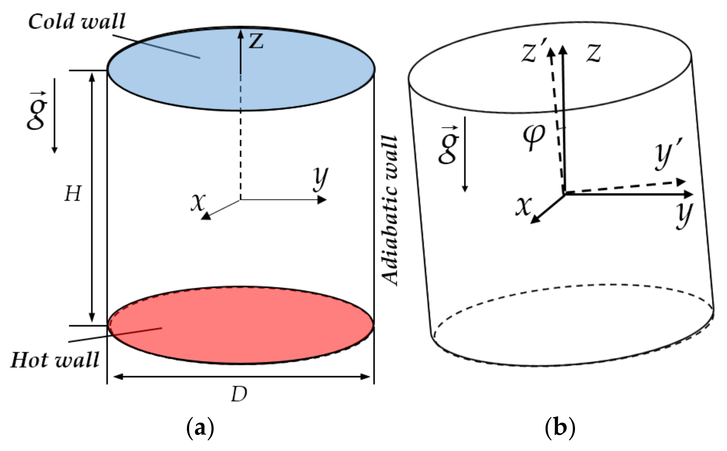
2.1. Rayleigh-Bénard Convection in a Cylinder

Direct numerical simulation of turbulent Rayleigh-Bénard convection was performed in vertical (Figure 2a) and tilted (Figure 2b) cylindrical cells with a diameter-to-height aspect ratio Γ = D/H = 1. The coordinate system has its origin in a center of the cylinder. Some details on the problem definition, as well as preliminary results, were reported by us in [37,38]. No-slip conditions are imposed on all boundaries. Constant temperatures were set on the horizontal walls. The lateral cylindrical surface was assumed adiabatic.

First, let us define the scales of the problem. As a linear scale, we take the height of the container H. The temperature scale is the temperature difference on the horizontal walls ΔT. For the scale of velocities, we choose the characteristic velocity of free convection (buoyancy velocity) V_b = (gβΔTH)^0.5. The time scale is the characteristic convective time t_b = H/V_b.

The heat and mass transfer in present configuration is determined by the Prandtl number, Pr, and the Rayleigh number, Ra, which are defined as follows:

$$\mathrm{Pr}=\frac{v}{a}, \mathrm{Ra}=\frac{\mathrm{Pr}\times g\beta \Delta T{H}^3}{v^2},$$

where ΔT = T_h–T_c is the temperature difference between hot and cold walls.

In present study, we consider the case of Pr = 6.4, Ra = 10⁸.

Here, we also investigate the effect of tilting the container at a small angle relative to the gravity vector (φ = 2°) in the plane y0z.

2.2. Convection of an Internally Heated Fluid

Figure 3 shows the computational domain: a horizontal layer of fluid of height H, bounded above and below by plates of equal temperatures T = 0 (here, the temperature is measured from the reference one), that is subject to volumetric uniform heating Q. The lateral boundaries of the domain are periodic in corresponding directions. The lengths of the domain in both periodic directions are equal to L; we consider two cases: Γ = L/H = 1 and Γ = 2 (the origin of the coordinate system is located at the center of the domain). Note that the problem definition presented here is based on the paper [52].

As a linear scale, we take the layer height, H. For the scales of velocity and time, we choose the V_b = (gβQH³/a)^0.5 and t_b = H/V_b, respectively. Temperature scale is chosen according to the paper [52] as T_b = H²Q/a.

The heat and mass transfer in present configuration is determined by the Prandtl number and Rayleigh number, latter is defined as follows:

$$\mathrm{Ra}=\frac{\mathrm{Pr}\times g\beta Q{H}^5}{a{v}^2}$$

In present study, we consider the case of Pr = 1, Ra = 10¹⁰.

2.3. Computational Aspects

Numerical simulations were performed using in-house finite-volume code SINF/Flag-S developed at Peter the Great St. Petersburg Polytechnic University; the code can operate with unstructured grids. We used a variation of the fractional step method described in [56]. The Crank–Nicolson scheme with second-order accuracy was used for advancing in time. In cylindrical container, a central difference scheme was used to approximate the convection terms in the governing equations. Spatial discretization of the convective terms is performed with the third-order QUICK scheme for convection of an internally heated fluid. The diffusion terms were approximated by the central-difference scheme of the second order accuracy.

For the case of convection in cylinder, we used a computational grid consisting of hexagonal elements with about 15 mln cells. For the internally heated convection, we used structured grids: “rough” grid of size 2 mln cells and “fine” grid of size 4 mln cells for Γ = 1 and 16 mln cells for Γ = 2. The grids were clustered to the walls (the vertical cell dimension near the wall amounted to about 10^–4H).

Calculations of turbulent convection can be considered as direct numerical simulation of turbulent flow if the local cell size is of the same order or less than the size of the smallest vortex structures in a given region. It is known that in cases where the velocity layers are thinner than the temperature layers (Pr < 1), the smallest turbulence scale is the Kolmogorov scale

$${\delta }_K={\left(\frac{v^3}{\epsilon }\right)}^{0.25}{\mathsf{\delta }}_{\mathrm{K}}=({\mathsf{\nu }}^3/\mathsf{\epsilon }{)}^{0.25},$$

where ε is the dissipation rate of kinetic energy

$$\epsilon =\nu \overline{\frac{\partial V_i\text{'}}{\partial x_k}\frac{\partial V_i\text{'}}{\partial x_k}},$$

where V_i′—is the fluctuation of the i-th velocity component. For Pr > 1, the smallest scale is the Batchelor scale

$${\delta }_B=\frac{{\delta }_K}{P{r}^{0.5}}$$

Thus, to assess the quality of the calculations, it is necessary to compare the characteristic size of the grid cells with one or another minimum scale of the turbulent flow.

We actually analyzed the fields of the Kolmogorov and Batchelor scales computed by the above relations and taken relative to the cubic root of the computational cell volume (Vol^1/3). After performed calculations, it was found that in almost the entire convection region, ratios Vol^1/3/δ_K and Vol^1/3/δ_B assumed values less than one. In the case of convection in the cylindrical container, the exception was a small region near the adiabatic wall in the middle-height layer, as well as the location of angular vortices, where the maximum ratios Vol^1/3/δ_B were approximately 1.4. In the case of internally heated convection, the maximum ratios Vol^1/3/δ_K and Vol^1/3/δ_B were observed in the middle-height layer and were approximately 2.

Thus for both cases the cell size exceeded the minimum turbulence scale only within the restricted areas of the regions, and at the most by factor 2. In our previous studies [37,38], it was shown that such degree of resolution of the turbulent content is sufficient to obtain grid-independent fields of average velocity and temperature, as well as pulsation values characterizing small-scale turbulence (this will also be illustrated in the present study).

The time step did not exceed one hundredth of the characteristic time t_b and was noticeably less than the Kolmogorov time scale t_K = (ν/ε)^0.5 in the entire region for all cases considered.

3. Results

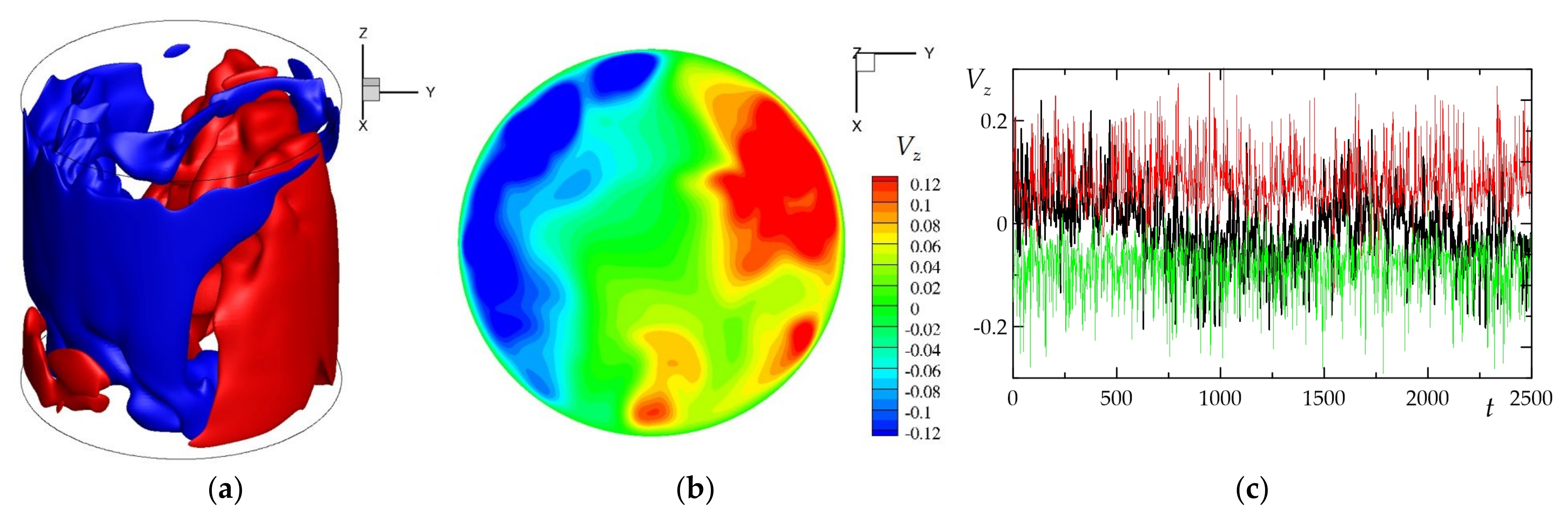
3.1. Rayleigh-Bénard Convection in a Cylinder

First, we consider the case of convection of water in a vertical oriented cylindrical cell. Figure 4a,b, illustrates an instantaneous picture of convection: the presence of the large-scale coherent structure is clearly seen. In non-tilted container, this CS can perform azimuthal motion. Temporal changes in the dimensionless vertical velocity component at the point located at the distance of 0.17D from the sidewall are shown in Figure 4c (black line). These changes are due to the large-scale coherent structure azimuthal reorientations. It can be seen that in non-tilted container, after about a certain period, the CS begins to slowly rotate, thus changing its azimuthal position; thus, here the flow reversals of the CS are due to its azimuthal reorientations. In Figure 4c, we also present the results for the tilted container, where CS is fixed: green and red lines correspond to the temporal dependence of the dimensionless vertical velocity component at two points located symmetrically in the regions of ascending (red line) and descending (green line) flows. Here, it is clearly seen that the random azimuthal reorientations of CS, as well as flow reversals, are almost absent; the CS can perform only slight azimuthal oscillations near its average position.

Due to random azimuthal instability of the CS in case of non-tilted container, the degree of spatial inhomogeneity of the vertical velocity field in the central horizontal section averaged over a sufficiently large time sample (Figure 5a) is cardinally reduced compared to the instantaneous field (Figure 4b). Theoretically, for a large enough arbitrary sample, the time-average velocity in the given section and in the whole region should be zero.

Figure 5b,c illustrates the averaged vertical velocity distributions obtained for a container tilted by 2°. Hereinafter, the “vertical velocity component” means the velocity component along the axis of the tilted container. It is seen that this distribution is characterized by double symmetry: relative to line 2 and the central vertical plane passing through line 1. This is to be expected in the case of the CS “fixed” in a certain azimuthal orientation. Due to the absence of low-frequency azimuthal oscillations of the CS, a sample of 400t_b turns out to be sufficient to obtain reliable statistics for the modeled Rayleigh-Bénard convection.

It is of interest to determine the characteristics of the convective flow in the central vertical section of the container, coinciding with the central section of CS (it is a plane tilt y′0z′). As shown in paper [38], in addition to the large-scale CS, a number of smaller angular vortices are observed which are located in the corners of the container. Such flow structure is consistent with the distribution of the kinetic energy of turbulence in the central vertical plane shown in Figure 6. In the regions of interaction of angular vortices with the CS, the most intense velocity pulsations are present. In the center of the cylinder, the level of pulsations is noticeably lower.

As noted in the Introduction, random changes in the orientation of the CS greatly complicate the process of obtaining the distributions of physical quantities characterizing small-scale background turbulence. In particular, Figure 6a illustrates how strongly the velocity pulsates, and, consequently, the kinetic energy increase in the presence of azimuthal oscillations in comparison with the case of a “fixed” CS (Figure 6b,c).

As a result of the calculations performed for the “fixed” CS, three-dimensional fields of all components of the Reynolds stress tensor and the vector of turbulent heat flux were also obtained (Figure 7). The lines 1 and 2 in the central horizontal section of the container, along which the data in Figure 7 are presented, as shown in Figure 5c. Note that a large amount of data and a detailed analysis of the results are presented in paper [38]. The illustrated distributions are obtained after averaging over two halves of each of the lines. It can be seen that the maxima of the correlations, which include the vertical component of the velocity (Figure 7c,d,f), are related exactly on the section of the mixing layer (x ≈ 0.95D). In the region of the most intense motion of the CS (y ≈ 0.95D), there is no sharp change in the correlations of the vertical velocity. Correlations of other velocity components are usually noticeably lower; they are characterized by a smoother change in the central horizontal plane (Figure 7a,b,e). In the center of the cylinder, as a rule, no intense pulsating motion is observed.

The integral heat transfer in the cases of vertically oriented and tilted cylinders turn out to be close to each other. In particular, the integral Nusselt number in the case of water convection at Ra = 10⁸ is 33.0, which agrees with an accuracy of three significant digits with the calculation result [57] performed within the DNS approach for a non-tilted container.

Thus, in case of the “fixed” CS, the characteristics of the large-scale coherent structure could be identified unambiguously. To perform the analysis of the anisotropy invariant map, we extract Reynolds stress data along several lines inside the computational domain: two lines pass through the domain center and lie in the central xy section (first line along y axis, and second line along x), third line also passes through domain center along vertical axis z, and fourth line passes through point x = 0, y = 0.4D along z line (these lines are schematically shown in corresponding figures). AIMs for the first two lines are shown in Figure 8, top row, for third and fourth lines—in Figure 8, bottom row. In Figure 8, top row, one can see that near the lateral walls turbulence is as in turbulent boundary layer, then, farther from the lateral wall, turbulence is getting closer to isotropic with transition between “rod-like” and “disk-like” archetypes. The turbulence near top and bottom walls of the cylinder, conversely, is mainly axisymmetric in center line and near axisymmetric for line at y = 0.4D (see Figure 8, bottom row). It is interesting to note that turbulence along vertical line changes its archetype from “disk-like” to “rod-like” as we move away from the wall. Such change in archetype can be explained as follows: near the wall, where boundary layer takes place, the fluctuations of the vertical velocity component is actively suppressed by the close proximity of the top/bottom walls, whereas fluctuations of the horizontal velocity components evolve. Such anisotropy is typical for the near-wall turbulence [58]. Far from the wall, turbulence becomes isotropic. But in the center of the cylinder, where ascending and descending flows are dominant, the vertical velocity component fluctuations also prevail over the horizontal ones.

We have also performed averaging of the turbulence anisotropy tensor over horizontal sections to obtain its distribution along vertical coordinate. In Figure 9 the corresponding AIM is shown. Averaging over horizontal sections clearly reveals the details of turbulence archetype under study: in the average, near the bottom and top walls of the cylinder the turbulence is 2D axisymmetric, then, turbulence remains axisymmetric but with tendency to isotropic, and turbulence in the center of the cylinder is mainly “rod-like”. Such behavior is most likely due to the presence of coherent vortex structure.

3.2. Convection of an Internally Heated Fluid

The typical instantaneous non-dimensional temperature distribution in the computational domain for two cases considered is shown in Figure 10 (temperature is scaled by T_b). One can see the cold thermals descending from above, which leads to intensive mixing near the top wall, and consequently the boundary layer is thin. Contrariwise, the boundary layer near the bottom wall is noticeably thicker. Such difference in the boundary layers thickness is clearly visible in the distribution of the mean temperature across whole domain (see Figure 11a). Note that mean characteristics are obtained by both averaging in time and in horizontal planes.

The mean temperature distribution shown in Figure 11a is in good agreement with the data presented in [52]. Obviously, the mean temperature does not depend on the periodic length L: the temperature distributions obtained for two cases considered are almost identical.

Figure 11b,c, shows the RMS of vertical and horizontal velocity components; one can see that “fine” grid is enough to obtain almost grid-independent results. It should be noted that similar distributions of velocity components RMS are presented in paper [52]; our results are in qualitative agreement with them.

Some non-uniformity is seen in RMS of horizontal velocity component distribution, Figure 11c; note also that RMS distributions differ markedly for different lengths L. Now, the nature of such in-homogeneity is not evident; perhaps, it is connected to emergence and reversals of the large-scale coherent structures in the flow.

As noted in Introduction, the presence of CS are reported by many authors for the classic turbulent Raylegh-Bénard convection. Here, such structures also take place. In Figure 12 the instantaneous distributions of the vertical velocity component are shown in central horizontal section at different times for the case Γ = 1. Three time moments are shown. First time moment (Figure 12a) corresponds to the presence of the quasi-2D coherent vortex structure: in the central part of the domain, the flow is descending in general, whereas a lifting motion takes place in other regions; note that descending motion is more intense that ascending one. The second time moment (Figure 12b) corresponds to the disruption of the large-scale coherent structure, and the third time (Figure 12c) corresponds to the emergence of the quasi-2D coherent structure that is orthogonal to that shown in Figure 12a. It should be noted that for the case Γ = 1 the “life time” of the coherent structure is short enough (less than 200t_b).

To perform identification of CS behavior (including the emergence, disruption, and re-orientation) more clearly, we have also performed the Fourier mode decomposition of the instantaneous velocity field described in [50] for three time moments corresponding to the times shown in Figure 12. Three-dimensional instantaneous velocity field (V_x, V_y, V_z) for each time moment was projected onto the Fourier basis, for which we choose 2D modes oriented in the xz or yz planes. Thus, we assume that flow field can be represented as a number of 2D vortices in two orthogonal horizontal directions. The number of these 2D vortices in vertical and horizontal directions corresponds to mode numbers (m, n, k), where m and n are the modes in horizontal directions (one of m or n should be set to zero to obtain 2D vortices), and k is the mode in vertical direction. Considering first three modes in each direction, we calculated the normalized energy of each mode (m, n, k) divided by the total energy to determine dominant Fourier modes. Our calculations showed that for the time moment corresponding to Figure 12a, one dominant mode (0, 2, 1) takes place with normalized energy of value 0.21; other Fourier modes have normalized energy less than 0.1. Thus, Fourier mode decomposition shows presence of the CS, which is represented by two 2D vortices in yz plane. For the time moment corresponding to Figure 12b, there is no single noticeable dominant mode: two modes (0, 1, 1) and (0, 2, 1) with normalized energy of about 0.13 take place, whereas other modes have normalized energy less than 0.1. Finally, for the time moment corresponding to Figure 12c, one dominant mode (2, 0, 1) takes place with normalized energy of 0.16, other modes have energy less than 0.1. In this case, we see two 2D vortices in xz plane. Thus, Fourier mode decomposition analysis also confirms the presence of the CS, its disruption and re-emergence in the orthogonal direction over time.

The emergence and evolution of the large-scale CS can be also seen in time dependence of vertical velocity component in the center of the domain, see Figure 13. Here, the low-frequency oscillation of the vertical velocity component corresponds to the emergence of the large-scale CS with different orientation and location in space.

It should be noted that in case Γ = 2 these large-scale oscillations have much lower frequency; thus, coherent structure turnover time is increasing, and we can perform averaging over the period of the large-scale structure existence to obtain Reynolds stress tensor. In Figure 14a and Figure 15b the fields of the instantaneous vertical velocity component and the one averaged by the period of coherent structure existence are presented (the averaging period is 200t_b; the figure is doubled in periodic directions for visibility). Of course, chosen averaging period does not allow to obtain fully time-independent means, however, obtained mean distributions can reveal some important details useful for the development of the methods of large-scale coherent structure identification.

Chosen for averaging time period was used to obtain the fields of the following turbulent characteristics: turbulent kinetic energy, turbulent dissipation, Reynolds stress tensor. In Figure 14b the distributions of the turbulent kinetic energy are shown (the pictures are doubled in periodic directions). Comparing with Figure 14a, one can see that the most intense turbulence oscillations take place in the region of descending flow and in the region between descending and ascending flows.

The large-scale coherent structure is clearly seen in Figure 15, where isosurfaces of the mean velocity and distribution of the vertical component of the mean velocity are shown (picture in Figure 15b is doubled in x and y directions). This coherent structure is apparently 2D vortex; it can move along periodic directions, which leads to flow reversals.

The anisotropy invariant map obtained for the different lines is shown in Figure 16 for the case Γ = 2. Here, we choose three lines: the first one lies in the horizontal central section and crosses CS, the second and third lines are vertical and located in the zones of descending flow and mixing layer between ascending and descending flows. Due to insufficient averaging time, the AIMs are more complicated than in case of convection in tilted cylinder. However, the main features can be identified. The first line (red color in Figure 16) crosses CS in the horizontal direction, and the turbulence archetype sequentially changes between “rod-like” and “disk-like” axisymmetric turbulence, but in general, turbulence is close to isotropic. AIMs for the second and third lines (blue and green colored) start and end in the region of 2D turbulence (near the bottom and top walls), and in the central part of the domain the turbulence archetype is also changes between “rod-like” and “disk-like”, and its anisotropy is more pronounced.

The most interesting result is the AIM for the distribution of the Reynolds stress tensor, averaged over horizontal sections, see Figure 17. Due to horizontal averaging in space, we obtain more statistically established distribution along vertical coordinates, and the turbulence archetype becomes very close to the one obtained for analogue distribution in case of tilted cylinder (compare with Figure 9). This is a very interesting result, which will be discussed below.

It is interesting to note that similar flow behavior takes place in Rayleigh-Bénard convection in a cubic cell [59], where large-scale CS changes its orientation due to cessation. We guess that similar steady (and unsteady) AIM analysis can be applied for the identification of CS, revealing its properties in space in time.

4. Discussion

In the present study, we investigate two quite different configurations of the convection of Rayleigh-Bénard type. First is the convection in a cylinder heated from below, which is very heavily studied by many other researchers, both experimentally and numerically. For this case, by means of our numerical simulation, we also have confirmed the presence of large-scale CS, which can rotate in azimuthal direction if the cylinder is not tilted. Such rotation of the CS leads to the flow reversals and to the difficulties in obtaining statistical properties of the turbulent motion. To prevent the CS from rotation, we use a modified problem statement with slightly tilted cylinder. In this case, the CS becomes “fixed” and can be easily visualized and investigated, and we have carried out the AIM analysis for this case, which shows characteristic behavior of turbulence archetype when moving between different regions of the CS.

Averaging of the Reynolds stress tensor across horizontal section leads to a quite simple AIM (shown in Figure 9), where three main regions of the different turbulence archetypes have place: first region corresponds to the areas near top and bottom walls where turbulence is mostly 2D axisymmetric. Second region is located between the wall and domain center, and the turbulence archetype there is close to isotropic. The last region is located in the central part of the domain, and it is characterized by the dominance of the “rod-like” axisymmetric turbulence. We guess that such archetype variance is due to the presence of the large-scale CS.

The second configuration considered is the internally heated convection in a layer. This case was also heavily studied by many authors (e.g., see [52]), but the analysis of the turbulence archetypes for such flows is almost absent. Of course, the existence of CS was mentioned in many papers, especially for the case of classical Rayleigh-Bénard convection (see the corresponding references in Introduction), but due to the high degree of freedom in periodic directions, these CS move quite occasionally in different horizontal directions, so their determination and investigation becomes very challenging. In our investigation, according to [52], we chose quite small computational domain in periodic directions, and we were able to detect the emergence of the CS and perform its analysis. It was established that emerging CS is very similar to the 2D vortices, which are elongated along one or another periodic direction, and CS is disrupted time to time with emergence of a new one, located orthogonally; performed Fourier mode decomposition analysis has confirmed our deductions. Furthermore, we saw that the descending motion in coherent structure is more intense that ascending one; such observation is consistent with the conclusion obtained in paper [60], where the Large Eddy Simulation has been carried out for the case of radiatively-driven convection in a lake; in our further studies, we plan to perform Direct Numerical Simulation of radiatively-driven convection to verify those results.

It was shown that in the computational domain of size Γ = 2, turnover time of CS is large enough, so we could perform more accurate averaging over the period of the large-scale structure existence. The analysis of the AIM for the case of internally heated convection shows that the spatial distribution of turbulence anisotropy parameters is highly variable (as in the case of convection in a cylinder): in some regions, the turbulence has “rod-like” structure, and in other—“disk-like” structure. Such behavior of the turbulence archetype is very close to the one for the case of convection in a cylinder. In Figure 18, two AIMs are shown, which correspond to the distributions along similar lines for two cases considered (convection in a cylinder and internally heated convection): the lines pass vertically through the mixing region between ascending and descending flows (green lines in Figure 8 and Figure 16). Some similar features are observed for two cases: first, anisotropy parameters of the turbulence vary between “rod-like” and “disk-like” limits as one moves away from the wall. Near the walls, the turbulence archetype is quite similar: both points 1 in Figure 18 lie on the top boundary of Lumley triangle, which corresponds to the 2D turbulence, but for the convection in a cylinder, the turbulent pulsations are nearly axisymmetric; of course, this is due to the different types of symmetry in the two problem definitions. Near the center of the both domains, the turbulence archetype is close to axisymmetric “disk-like”. One can see that turbulence in a central part of a cylinder is practically isotropic, while for the internally heated convection it is farther from the isotropic (this is also possible due to insufficient averaging).

The most interesting result is the anisotropy invariant maps for the vertical distribution of the Reynolds stress tensor, which is obtained by averaging both in time and over horizontal cross sections (Figure 9 and Figure 17). We see that both maps have very similar structure: near the top and bottom walls, the turbulence is almost 2D axisymmetric, then, when one moves away from the walls, turbulence becomes similar to the “disk-like” one and more isotropic. However, in the central part of the computational domain, the turbulence archetype becomes close to the “rod-like” one, both for cylinder and layer cases. We guess that in both cases such behavior is due to the presence of the specific large-scale coherent structures.

5. Summary

In the paper, we presented the results of the study of turbulent archetypes, typical for heat-induced forcing, which triggers gravitational instability and Rayleigh-Bénard type convection. It was shown that, accordingly with the data of other authors, such flows are self-organized with the presence of large-scale coherent structures. In the non-tilted cylinder, the CS is the single vortex, which is stable and can rotate azimuthally, whereas in a tilted cylinder the CS is “fixed” in space. In the layer, the quasi-2D CS can arise, exist for some time, disrupt, and then re-emerge again; the stability of these CS can be connected with its random horizontal motion and interaction with relatively small arising thermals. It was shown that the turbulence archetypes are very similar for two chosen types of forcing, and there are the distinct CS fingerprints on anisotropy invariant map. Thus, analyzing the AIM, one can obtain useful information about the presence of CS in the flow of Rayleigh-Bénard type and its characteristics. By performing unsteady AIM analysis, one can reveal the CS motion, cessation and re-starting, which potentially can be helpful, in particular, for understanding flow reversals. Our further investigation will be directed to studies of the CS in penetrative convection driven by inhomogeneous heating of the water column, which is a challenging and important topic from both a fundamental and practical point of view.

References

1. Gargett, A.E.; Grosch, C.E. Turbulence Process Domination under the Combined Forcings of Wind Stress, the Langmuir Vortex Force, and Surface Cooling. J. Phys. Oceanogr. 2014, 44, 44–67. [Google Scholar] [CrossRef]
2. Pope, S.B. Turbulent Flows; Cambridge University Press: Cambridge, MA, USA, 2000; 771p. [Google Scholar] [CrossRef]
3. Emory, M.; Iaccarino, G. Visualizing turbulence anisotropy in the spatial domain with componentality contours. Cent. Turbul. Res. Annu. Res. Briefs 2014, 123–138. [Google Scholar]
4. Bluteau, C.E.; Jones, N.L.; Ivey, G.N. Turbulent mixing efficiency at an energetic ocean site. JGR Oceans 2013, 118, 4662–4672. [Google Scholar] [CrossRef] [Green Version]
5. Ulloa, H.; Wüest, A.; Bouffard, D. Mechanical energy budget and mixing efficiency for a radiatively heated ice-covered waterbody. J. Fluid Mech. 2018, 852, R1. [Google Scholar] [CrossRef] [Green Version]
6. Maffioli, A.; Brethouwer, G.; Lindborg, E. Mixing efficiency in stratified turbulence. J. Fluid Mech. 2016, 794, R3. [Google Scholar] [CrossRef] [Green Version]
7. Lumley, J.L. Computational modeling of turbulent flows. Adv. Appl. Mech. 1978, 18, 123–176. [Google Scholar]
8. Choi, K.-S.; Lumley, J.L. The return to isotropy of homogeneous turbulence. J. Fluid Mech. 2001, 436, 59–84. [Google Scholar] [CrossRef]
9. Simonsen, A.J.; Krogstad, P.-A. Turbulent stress invariant analysis: Clarification of existing terminology. Phys. Fluids 2005, 17, 088103. [Google Scholar] [CrossRef] [Green Version]
10. Kunnen, R.P.J. Turbulent Rotating Convection; Technische Universiteit Eindhoven: Eindhoven, The Netherlands, 2008. [Google Scholar] [CrossRef]
11. Penna, N.; Coscarella, F.; D’Ippolito, A.; Gaudio, R. Anisotropy in the Free Stream Region of Turbulent Flows through Emergent Rigid Vegetation on Rough Beds. Water 2020, 12, 2464. [Google Scholar] [CrossRef]
12. Liu, Y.; Yan, H.; Lu, L.; Li, Q. Investigation of Vortical Structures and Turbulence Characteristics in Corner Separation in a Linear Compressor Cascade Using DDES. J. Fluids Eng. 2017, 139, 021107. [Google Scholar] [CrossRef]
13. Font, B.; Weymouth, G.D.; Nguyen, V.-T.; Tutty, O.R. Span effect on the turbulence nature of flow past a circular cylinder. J. Fluid Mech. 2019, 878, 306–323. [Google Scholar] [CrossRef]
14. Gargett, A.; Wells, J.; Tejada-Martínez, A.E.; Grosch, C.E. Langmuir supercells: A mechanism for sediment resuspension and transport in shallow seas. Science 2004, 306, 1925–1928. [Google Scholar] [CrossRef] [PubMed]
15. Smyth, W.D.; Moum, J.N. Anistropy of turbulence in stably stratified mixing layers. Phys. Fluids 2000, 12, 1343–1362. [Google Scholar] [CrossRef] [Green Version]
16. Ye, Q.Y.; Wörner, M.; Grötzbach, G. Modelling Turbulent Dissipation Correlations for Rayleigh-Bénard Convection Based on Two-Point Correlation Technique and Invariant Theory; Karlsruhe FZKA: Karlsruhe, Germany, 1998; 54p. [Google Scholar]
17. Brown, E.; Ahlers, G. Rotations and cessations of the large-scale circulation in turbulent Rayleigh–Bénard convection. J. Fluid Mech. 2006, 568, 351–386. [Google Scholar] [CrossRef] [Green Version]
18. Mishra, P.K.; De, A.K.; Verma, M.K.; Eswaran, V. Dynamics of reorientations and reversals of large-scale flow in Rayleigh–Bénard convection. J. Fluid Mech. 2011, 668, 480–499. [Google Scholar] [CrossRef] [Green Version]
19. Verma, M.K. Physics of Buoyant Flows: From Instabilities to Turbulence; World Scientific: Singapore, 2018; 352p. [Google Scholar] [CrossRef]
20. Kelley, D.E. Convection in ice-covered lakes: Effects on algal suspension. J. Plankton Res. 1997, 19, 1859–1880. [Google Scholar] [CrossRef]
21. D’Asaro, E.A. Convection and the seeding of the North Atlantic bloom. J. Marine Syst. 2008, 69, 233–237. [Google Scholar] [CrossRef]
22. Woodward, J.R.; Pitchford, J.W.; Bees, M.A. Physical flow effects can dictate plankton population dynamics. J. R. Soc. Interface 2019, 16, 20190247. [Google Scholar] [CrossRef] [PubMed] [Green Version]
23. Martinat, G.; Grosch, C.E.; Gatski, T.B. Modeling of Langmuir Circulation: Triple Decomposition of the Craik–Leibovich Model. Flow Turbul. Combust. 2011, 92, 395–411. [Google Scholar] [CrossRef]
24. Pernica, P.; North, R.L.; Baulch, H.M. In the cold light of day: The potential importance of under-ice convective mixed layers to primary producers. Inland Waters 2017, 7, 138–150. [Google Scholar] [CrossRef]
25. Ahlers, G.; Grossmann, S.; Lohse, D. Heat transfer and large-scale dynamics in turbulent Rayleigh-Bénard convection. Rev. Mod. Phys. 2009, 81, 503–538. [Google Scholar] [CrossRef] [Green Version]
26. Chillà, F.; Schumacher, J. New perspectives in turbulent Rayleigh-Bénard convection. Eur. Phys. J. E 2012, 35, 1–25. [Google Scholar] [CrossRef] [PubMed] [Green Version]
27. Wu, X.-Z.; Libchaber, A. Scaling relations in thermal turbulence: The aspect-ratio dependence. Phys. Rev. A 1992, 45, 842–845. [Google Scholar] [CrossRef]
28. Cioni, S.; Ciliberto, S.; Sommeria, J. Experimental study of high-Rayleigh-number convection in mercury and water. Dyn. Atmos. Oceans 1996, 24, 117–127. [Google Scholar] [CrossRef]
29. Niemela, J.J.; Skrbek, L.; Sreenivasan, K.R.; Donnelly, R.J. Turbulent convection at very high Rayleigh numbers. Nature 2000, 404, 837–840. [Google Scholar] [CrossRef] [PubMed]
30. Ahlers, G.; Bodenschatz, E.; Funfschilling, D.; Hogg, J. Turbulent Rayleigh–Bénard convection for a Prandtl number of 0.67. J. Fluid Mech. 2009, 641, 157–167. [Google Scholar] [CrossRef] [Green Version]
31. Verzicco, R.; Camussi, R. Numerical experiments on strongly turbulent thermal convection in a slender cylindrical cell. J. Fluid Mech. 2003, 477, 19–49. [Google Scholar] [CrossRef]
32. Shishkina, O.; Thess, A. Mean temperature profiles in turbulent Rayleigh–Bénard convection of water. J. Fluid Mech. 2009, 633, 449–460. [Google Scholar] [CrossRef] [Green Version]
33. Scheel, J.D.; Kim, E.; White, K.R. Thermal and viscous boundary layers in turbulent Rayleigh–Bénard convection. J. Fluid Mech. 2012, 711, 281–305. [Google Scholar] [CrossRef]
34. Chillà, F.; Rastello, M.; Chaumat, S.; Castaing, B. Long relaxation times and tilt sensitivity in Rayleigh-Bénard turbulence. Eur. Phys. J. B. 2004, 40, 223–227. [Google Scholar] [CrossRef]
35. Ahlers, G.; Brown, E.; Nikolaenko, A. The search for slow transients, and the effect of imperfect vertical alignment, in turbulent Rayleigh–Bénard convection. J. Fluid Mech. 2006, 557, 347–367. [Google Scholar] [CrossRef] [Green Version]
36. Xi, H.-D.; Xia, K.-Q. Azimuthal motion, reorientation, cessation, and reversal of the large-scale circulation in turbulent thermal convection: A comparative study in aspect ratio one and one-half geometries. Phys. Rev. E 2008, 78, 036326. [Google Scholar] [CrossRef] [PubMed]
37. Smirnov, S.I.; Abramov, A.G.; Smirnov, E.M. Numerical simulation of turbulent Rayleigh-Bénard mercury convection in a circular cylinder with introducing small deviations from the axisymmetric formulation. J. Phys. Conf. Ser. 2019, 1359, 012077. [Google Scholar] [CrossRef]
38. Smirnov, S.I.; Smirnov, E.M. Direct numerical simulation of the turbulent Rayleigh-Bénard convection in a slightly tilted cylindrical container. St. Petersburg State Polytech. Univ. J. Phys. Math. 2020, 13, 14–25. [Google Scholar] [CrossRef]
39. Zwirner, L.; Khalilov, R.; Kolesnichenko, I.; Mamykin, A.; Mandrykin, S.; Pavlinov, A.; Shestakov, A.; Teimurazov, A.; Frick, P.; Shishkina, O. The influence of the cell inclination on the heat transport and large-scale circulation in liquid metal convection. J. Fluid Mech. 2020, 884, A18. [Google Scholar] [CrossRef] [Green Version]
40. Goluskin, D. Internally Heated Convection and Rayleigh-Bénard Convection; Springer Briefs in Thermal Engineering and Applied Science; Springer: Berlin/Heidelberg, Germany, 2016; 66p. [Google Scholar] [CrossRef]
41. Kerr, R.M.; Herring, J.R. Prandtl number dependence of Nusselt number in direct numerical simulations. J. Fluid Mech. 2000, 419, 325–344. [Google Scholar] [CrossRef]
42. Hartlep, T.; Tilgner, A.; Busse, F.H. Large Scale Structures in Rayleigh-Bénard Convection at High Rayleigh Numbers. Phys. Rev. Lett. 2003, 91, 064501. [Google Scholar] [CrossRef] [PubMed]
43. Pandey, A.; Scheel, J.D.; Schumacher, J. Turbulent superstructures in Rayleigh-Bénard convection. Nat. Commun. 2018, 9, 1–11. [Google Scholar] [CrossRef] [PubMed] [Green Version]
44. Hardenberg, J.V.; Parodi, A.; Passoni, G.; Provenzale, A.; Spiegel, E.A. Large-scale patterns in Rayleigh–Bénard convection. Phys. Lett. A 2008, 372, 2223–2229. [Google Scholar] [CrossRef]
45. Stevens, R.J.A.M.; Blass, A.; Zhu, X.; Verzicco, R.; Lohse, D. Turbulent thermal superstructures in Rayleigh-Bénard convection. Phys. Rev. Fluids 2018, 3, 041501. [Google Scholar] [CrossRef]
46. Berkooz, G.; Holmes, P.; Lumley, J.L. The proper orthogonal decomposition in the analysis of turbulent flows. Annu. Rev. Fluid Mech. 1993, 25, 539–575. [Google Scholar] [CrossRef]
47. Petschel, K.; Wilczek, M.; Breuer, M.; Friedrich, R.; Hansen, U. Statistical analysis of global wind dynamics in vigorous Rayleigh–Bénard convection. Phys. Rev. E 2011, 84, 026309. [Google Scholar] [CrossRef] [PubMed] [Green Version]
48. Xu, A.; Chen, X.; Wang, F.; Xi, H.-D. Correlation of internal flow structure with heat transfer efficiency in turbulent Rayleigh–Bénard convection. Phys. Fluids 2020, 32, 105112. [Google Scholar] [CrossRef]
49. Bhattacharya, S.; Verma, M.K.; Samtaney, R. Prandtl number dependence of the small-scale properties in turbulent Rayleigh-Bénard convection. Phys. Rev. Fluids 2021, 6, 063501. [Google Scholar] [CrossRef]
50. Xu, A.; Chen, X.; Xi, H.-D. Tristable flow states and reversal of the large-scale circulation in two-dimensional circular convection cells. J. Fluid Mech. 2021, 910, A33. [Google Scholar] [CrossRef]
51. Kulacki, F.A.; Goldstein, R.J. Thermal convection in a horizontal fluid layer with uniform volumetric energy sources. J. Fluid Mech. 1972, 55, 271–287. [Google Scholar] [CrossRef]
52. Goluskin, D.; van der Poel, E.P. Penetrative internally heated convection in two and three dimensions. J. Fluid Mech. 2016, 791, R6. [Google Scholar] [CrossRef] [Green Version]
53. Lepot, S.; Aumaître, S.; Gallet, B. Radiative heating achieves the ultimate regime of thermal convection. Proc. Natl. Acad. Sci. USA 2018, 115, 8937–8941. [Google Scholar] [CrossRef] [Green Version]
54. Bouillaut, V.; Lepot, S.; Aumaître, S.; Gallet, B. Transition to the ultimate regime in a radiatively driven convection experiment. J. Fluid Mech. 2019, 861, R5. [Google Scholar] [CrossRef]
55. Creyssels, M. Model for classical and ultimate regimes of radiatively driven turbulent convection. J. Fluid Mech. 2020, 900, A39. [Google Scholar] [CrossRef]
56. Smirnov, S.I.; Smirnov, E.M.; Smirnovsky, A.A. Endwall heat transfer effects on the turbulent mercury convection in a rotating cylinder. St. Petersburg Polytech. Univ. J. Phys. Math. 2017, 3, 83–94. [Google Scholar] [CrossRef]
57. Kooij, G.L.; Botchev, M.A.; Geurts, B.J. Direct numerical simulation of Nusselt number scaling in rotating Rayleigh–Bénard convection. Int. J. Heat Fluid Flow 2015, 55, 26–33. [Google Scholar] [CrossRef]
58. Ahn, J.; Kim, K.-H.; Pan, X.; Choi, J.-I. Contribution of Reynolds shear stress to near-wall turbulence in Rayleigh–Bénard convection. Int. J. Heat Mass Transfer 2021, 181, 121873. [Google Scholar] [CrossRef]
59. Vasilev, A.; Frick, P.; Kumar, A.; Stepanov, R.; Sukhanovskii, A.; Verma, M.K. Transient flows and reorientations of large-scale convection in a cubic cell. Int. Commun. Heat Mass Transf. 2019, 108, 104319. [Google Scholar] [CrossRef] [Green Version]
60. Mironov, D.; Danilov, S.; Olbers, D. Large-eddy simulation of radiatively-driven convection in ice-covered lakes. In Proceedings of the 6th International Workshop on ‘Physical Processes in Natural Waters’, Girona, Spain, 27–29 June 2001; pp. 71–75. [Google Scholar]
Figure 1. Lumley triangle: different archetypes of the turbulence on the map of the turbulence anisotropy tensor invariants.
Fluids 06 00431 g001
Figure 2. Computational domain for: (a) original geometry for Rayleigh-Bénard convection in a cylinder, (b) the tilted cylinder case. H—cylinder height, D—cylinder diameter.
Fluids 06 00431 g002
Figure 3. Computational domain: H—domain height, L—length in periodic directions. Top and bottom walls have equal temperature T = 0.
Fluids 06 00431 g003
Figure 4. (a) Instant vertical velocity isosurfaces (the red color corresponds to the ascending flow with Vz = +0.06Vb, the blue color corresponds to the descending flow with Vz = −0.06Vb); (b) instantaneous field of the dimensionless vertical velocity component in the central horizontal section; (c) temporary changes in the dimensionless vertical velocity component at a point located near the sidewall for the non-tilted container (black line), and the temporal dependence of the dimensionless vertical velocity component at two points located symmetrically in the regions of ascending (red line) and descending (green line) flows for the tilted container.
Fluids 06 00431 g004
Figure 5. Time-averaged fields of the dimensionless vertical velocity component in the central horizontal section: (a) vertical container (averaging time 2500tb); (b) tilted container (averaging time 400tb); (c) tilted container (averaging time 4000tb).
Fluids 06 00431 g005
Figure 6. Dimensionless kinetic energy of turbulence in the central horizontal section: (a) vertical container (averaging time 2500tb); (b) tilted container (averaging time 400tb); (c) tilted container (averaging time 4000tb).
Fluids 06 00431 g006
Figure 7. Changes in the normalized components of the Reynolds stress tensor (ad) and the turbulent heat flux vector (e,f) along the radial coordinate: black curves—along line 2, red curves—along line 1 (see Figure 5c), coordinate r = 0 corresponds to the point (x, y′, z′) = (0, 0, 0).
Fluids 06 00431 g007aFluids 06 00431 g007b
Figure 8. AIM for convection in a titled cylinder along different lines. (a) variables II, III (b) variables η, ζ. Points 1, 2, 3 correspond to the start point in a line, to the point at ¾ of line length, and to the point at ½ of line length. The lines are schematically shown on the small picture with CS in cylinder: in the top row, the lines lie in xy central section; in the bottom row, lines lie in yz central section.
Fluids 06 00431 g008
Figure 9. AIM for convection in titled cylinder: the averaged in horizontal section distribution over vertical coordinate: (a) variables II, III (b) variables η, ζ. Points 1 and 2 correspond to bottom section and central section of the cylinder.
Fluids 06 00431 g009
Figure 10. Non-dimensional temperature distribution in central xz cross section: (a) Г = 1; (b) Г = 2. Color legends are the same for both distributions.
Fluids 06 00431 g010
Figure 11. Vertical distributions of non-dimensional mean characteristics across the domain: (a) mean temperature; (b) RMS of vertical velocity component; (c) RMS of horizontal velocity component.
Fluids 06 00431 g011
Figure 12. Instantaneous dimensionless vertical velocity component distributions in horizontal section at different times for the case Г = 1: (a) time ~100tb; (b) time ~300tb; (c) time ~500tb.
Fluids 06 00431 g012
Figure 13. Time dependence of the dimensionless vertical velocity component at central point of the domain, case Г = 1.
Fluids 06 00431 g013
Figure 14. (a) Distributions of instantaneous dimensionless vertical velocity component, (b) dimensionless turbulent kinetic energy in central horizontal section z = 0 for the case Г = 2. The pictures are doubled in x and y directions for clarity.
Fluids 06 00431 g014
Figure 15. (a) Time-averaged vertical velocity isosurfaces (the red/blue colors correspond to the upward (Vz = 0.007Vb)/downward (Vz = −0.012Vb) flow), (b) time-averaged dimensionless vertical velocity averaged by coherent-structure existence period distribution for the case Г = 2, central section z = 0; the picture is doubled in x and y directions.
Fluids 06 00431 g015
Figure 16. AIM for internally heated convection along different lines. (a) variables II, III (b) variables η, ζ. Points 1 and 2 correspond to start point in line and to central point of line. Lines are schematically shown on the small picture.
Fluids 06 00431 g016
Figure 17. AIM for internally heated convection: the averaged in horizontal sections distribution over vertical coordinate: (a) variables II, III (b) variables η, ζ. Points 1 and 2 correspond to bottom section and central section of the domain.
Fluids 06 00431 g017
Figure 18. Anisotropy invariant maps both for convection in a cylinder (cyan lines) and internally heated convection (magenta lines): (a) variables II, III (b) variables η, ζ. The maps are constructed for the similar lines, which pass vertically through the mixing region of ascending and descending flows. Points 1 and 2 correspond to the bottom wall and a half of computational domain.
Fluids 06 00431 g018
Publisher’s Note: MDPI stays neutral with regard to jurisdictional claims in published maps and institutional affiliations.