Abstract
Impinging jets are of high interest in many industrial applications and their flow dynamics has a complex three-dimensional behavior. These jets can result in a high noise generation leading to acoustic discomfort. Thus, a passive control mechanism which consists of introducing a thin rod in the flow of the jet is proposed in order to reduce the noise generation. The stereoscopic particle image velocimetry (SPIV) technique is employed to measure the three velocity components in a plane. An experimental difficulty is encountered to acquire images of the flow in the shadow of the rod which block a part of the field of interest. In this paper, an experimental arrangement is proposed in order to overcome this experimental difficulty using a combined SPIV technique denoted by (C-SPIV). This technique consists of using an inclined mirror to illuminate the area under the rod by reflecting the laser light and two independent systems of SPIV synchronized and correlated together in order to obtain the combined field of velocity in the same plane above and below the rod. The C-SPIV measurements allowed to obtain the kinematic field in the whole area of interest. Thus, vortex shedding frequency, Turbulent Kinetic Energy were calculated and analyzed along with the acoustic signal. These results are of high interest when seeking for noise reduction in such jet configuration.
1. Introduction
Jet flow has been considered an interesting subject in the research field, because of its wide industrial application, such as in aeronautics and mechanical building systems. There are two main types of jet depending on the nozzle’s geometry: axisymmetric jet and asymmetric jet [1]. The most commonly used type of asymmetric jet is the rectangular jet that has several applications. A popular example is the air conditioning systems, where the ducts have a rectangular section and the jets impacting the diffuser are considered as rectangular jets. The complexity of studying jet dynamics is due to the presence of multi-scale vortical structures, which generally characterize the jet flow behavior. To understand the jet flow dynamics, several studies have been conducted [2,3,4,5,6,7,8,9]. These studies can be classified into three approaches: (1) analytical, which uses the Navier–Stock equation to determine the velocity field of the jet flow, (2) numerical, which is usually based on the finite volume method, and (3) experimental approach. The analytical approach is limited to the simplest of cases and cannot be used for complex flow behavior, in which cases the numerical and experimental approaches are recommended. The experimental works are based on different techniques of velocity measurement. Early experimental investigations were based on the Hotwire anemometry (HWA) and the Laser Doppler anemometry (LDA), which were used in the study of [10], to measure the velocity in a plane turbulent air jet at moderate Reynolds number. Advancingly, Pulsed Light Velocimetry techniques have emerged [11]; these methods consist of a pulsed sheet of light synchronized with a digital camera to take pictures when the light is pulsed. Tracer particles are often introduced in the flow to scatter the light to the camera lens. Using this approach, we can distinguish between Laser Speckle Velocimetry (LSV) and Particle Image Velocimetry (PIV), which differ in the concentration of scatters particles; the LSV is characterized by a high number of scatters particles, instead, in the PIV, the number of scatters is lower. These techniques have been performed in the work of [12], who used the digital version of PIV, applied to low-speed flow, and compared the results to that obtained using conventional LSV. The digital PIV was also performed in the study of [13], who compared the different post-processing techniques such as such as cross-correlation, direct spatial domain correlation, FFT, dynamic FFT, and hybrid correlation. More recently, Ref. [14] developed high image density PIV using laser scanning techniques to describe unsteady separated flows. Another technique has been developed by [15], who used the PIV and HWA techniques to identify the turbulence structures of pre-mixed impinging jets. In addition, Refs. [8,16] investigated the wall shear stress and the vortex dynamics in a circular impinging jet using a time-resolved PIV (TR-PIV) and polarography. Several types of PIV systems were proposed, depending on the number of dimensions (2D or 3D) and the number of velocity components (2C or 3C) studied by authors. The typical PIV system consists of one camera, so two velocity components are obtained in a plane (2D, 2C) [17]. Whereas the stereoscopic PIV (SPIV) consists of two cameras, that allow obtaining the third component of the velocity field in a plane (2D, 3C). The latter technique was illustrated by [18]. The most advanced type is the tomographic PIV that gives the three velocity components in a volume (3D, 3C). A detailed comparison between the tomographic PIV and the typical PIV was presented in the work of [19]. Likewise, in their study, Ref. [20] used the high-speed 3D tomographic to identify the turbulent kinetic energy in an impinging jet. In [21], a dual-plane stereo particle image velocimetry for measuring velocity gradient fields at intermediate and small scales of turbulent flows has been used. One should thus distinguish between a single plane SPIV, dual-plane SPIV, and multi-plane SPIV.
In certain configurations, impinging jets could produce a high level of noise, causing acoustic discomfort [22,23,24,25,26]. As a result, a passive control system that involves an insertion of a thin rod of 4 mm diameter into the jet’s flow to minimize noise generation was employed in a previous study [27]. To investigate the flow dynamics accompanied by this acoustic attenuation, we employ the SPIV for measurement in a single plane. However, when the rod is introduced in the flow, two issues arise: the first is depriving the area below the rod of light, the second is that illuminated particles targeted by the first camera cannot be seen by the second camera because of the presence of the rod. Thus, combined-SPIV (C-SPIV) measurements in the same plane is proposed using two independent synchronized SPIV systems. Therefore, in this paper, the C-SPIV technique is developed and implemented in order to obtain the velocity field of a rectangular air jet around the thin rod in the whole field of interest.
2. Materials and Methods
The experimental setup is shown in Figure 1a. A rectangular subsonic air jet, of Re = 5900 that corresponds to frequency peak, impinges on a slotted plate, with an impact ratio of L/H = 4, where L is the distance between the plate and the nozzle, and H is the height of the slot. This arrangement results in a flow that generates self-sustaining tones. A total of 1085 rod positions were tested between the nozzle and the impinging plate in order to identify the optimum rod position [27]. In order to understand the influence of the rod on the flow dynamics, we installed a combined stereoscopic PIV (C-SPIV) set up allowing us to measure the whole kinematic field of the flow around the rod. The C-SPIV requires the use of 4 cameras (3 Phantom V 711 and 1 Phantom VEO 710 are used in our study) of which two cameras have been installed above the rod and two cameras below the rod. For the SPIV measurements, the flow is seeded by olive oil particles (tracers) using an oil particle generator, which has an oil-air atomizer sprayed by a “Laskin Nozzle” aerographic system marketed by “Lavision”. The size of the seeded particles is measured by the “Topas” machine, it varies between 0.1 µm and 0.2 µm. For the lighting system, Litron Nd: YLF LDY 304-PIV laser having two heads of 30 mJ/pulse at a frequency of 1 KHz and a wavelength λ = 527 nm is used. The laser light beam is carried by a laser arm to illuminate the area between the jet nozzle and the plate. This laser arm contains 7 mirrors capable of operating for the wavelengths used, so it transmits 96% of the light intensity. The laser beam is transformed into a laser sheet by a sheet generator. The laser sheet generator contains both spherical and cylindrical lenses; the spherical lens allows the adjustment of the laser thickness and the cylindrical lens, its opening angle. The thickness of this laser light sheet and its opening angle can be adjusted depending on the divergent lens used. In addition, these lenses must withstand the high light power generated by the laser. In our case, we used a divergent lens with a focal length of 10 mm. Once the laser sheet has been generated, images can be acquired; a couple of images at instants t and t + Δt will be used to calculate the velocity field of the flow studied at a specific instant. The synchronization between the laser pulses and the camera apertures is controlled by a high-speed controller (HSC) from “Lavision”. This HSC has a maximum frequency of 50 KHz and can control four cameras simultaneously. The choice of the acquisition frequency depends on the phenomenon being studied. However, the choice of the time delay Δt between the two frames should be optimized to minimize the related error during image processing. Thus, Δt is chosen whereby to obtain a displacement of the particles in the fastest zone of the flow is between 5 and 10 pixels. The four cameras have CMOS sensors with a maximum resolution of 1200 × 800 pixels2. They are equipped with “Tokina” Macro lenses with a focal length equal to 100 mm and a maximum aperture that can be set to 𝑓/2.8. For Phantom 𝑉711 cameras and this image resolution, a maximum acquisition rate of 7530 frames per second can be achieved, while for Phantom 𝑉𝐸𝑂710 cameras, the maximum sampling rate is 7400 frames per second at the maximum spatial resolution [28]. These cameras are also equipped with Scheimpflug to adjust the image and lens planes with the laser sheet plane (object plane).
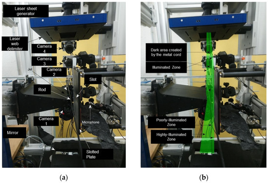
Figure 1.
(a) Illustration of the experimental setup consisting of combined SPIV. (b) Representation of different illuminated zones obtained by the introduction of the cord.
Once the images have been acquired, a routine must be applied to calculate the velocity field [29,30,31]. The SPIV measurement requires calibration to obtain accurate results. Therefore, a 3D double-sided plate was used in order to calibrate SPIV measurements without moving the calibration target. The reconstruction of the three-dimensional velocity field was done using the Davis 10.1.0 software which allows a stereoscopic reconstruction of the velocity vector of the two cameras in order to obtain the three velocity components of the flow.
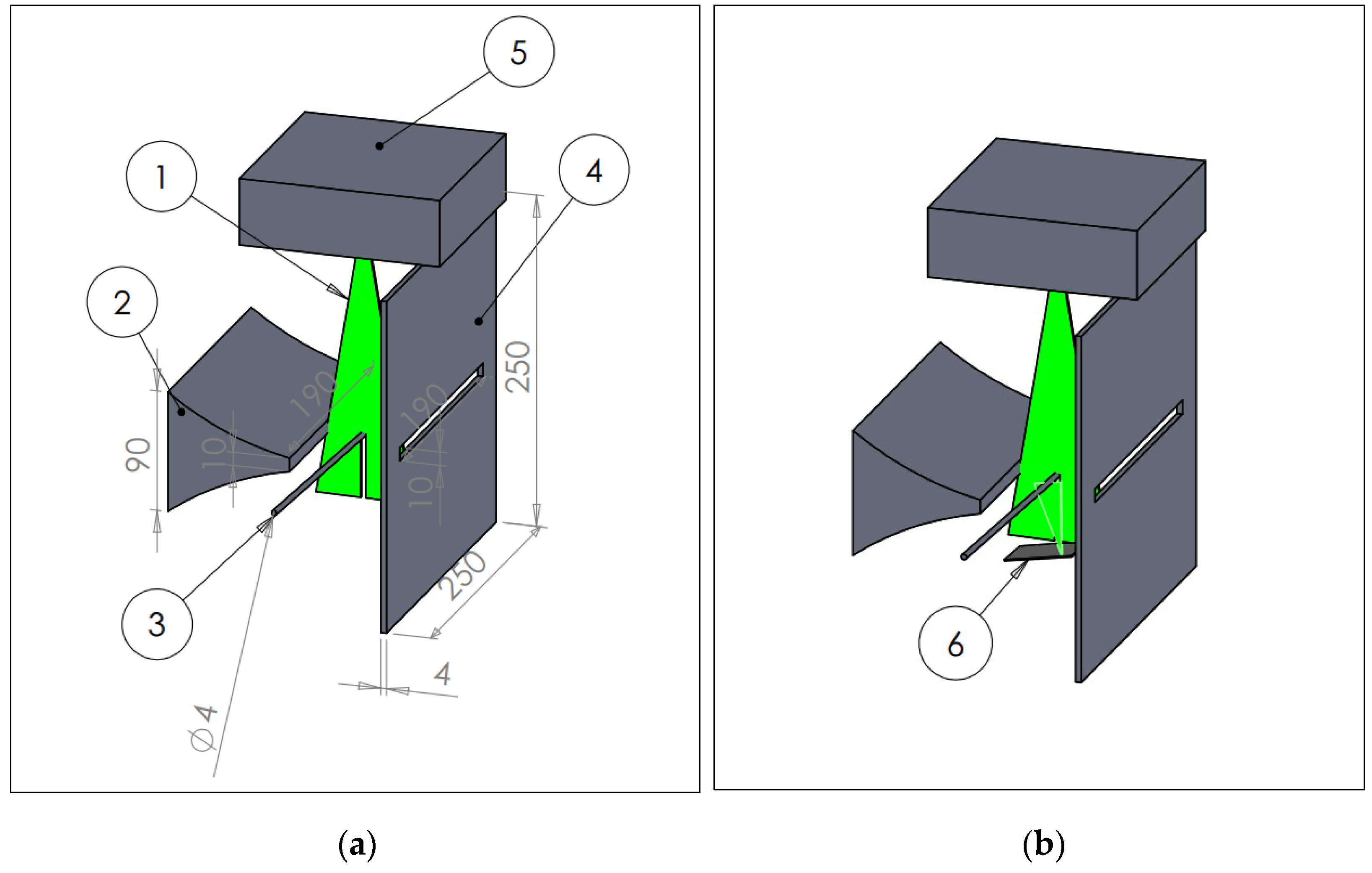
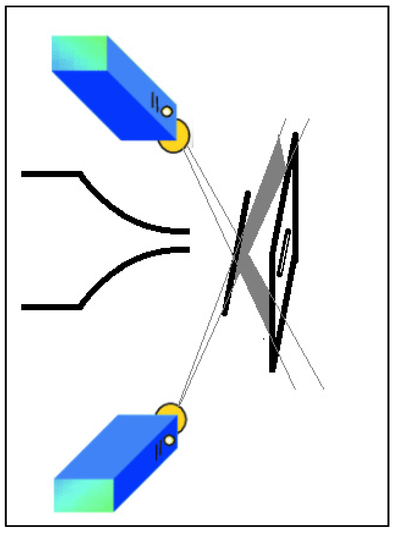
When applying the SPIV measurement to the configuration shown in Figure 1, two issues arise with the introduction of the rod. The first is due to the rod shadow in the lower part of the flow which prevents the application of the cross-correlation technique in this area (Figure 1b and Figure 2a). To overcome this difficulty, a mirror is installed below the rod to reflect the laser and illuminate the obscured area. This mirror must be tilted at an angle α to illuminate the dark area so that the reflected laser sheet is in the same plane as the incident laser and illuminates the dark area below the rod as seen in Figure 2. In addition, the mirror must be away from the flow area to not disturb the vortex dynamics.

Figure 2.
Illustration of the introduction of a mirror to illuminate the dark area below the rod (a) without a mirror; (b) with mirror. (1) Laser sheet, (2) nozzle, (3) rod, (4) slotted plate, (5) laser generator, (6) mirror.
Since the part located below the rod is less luminous than the upper part of the rod, the power of the laser has been increased to obtain sufficient illumination in this area, ensuring good correlations between particles when processed to obtain the kinematic field. It should be however noted that the increased laser power causes another problem due to the reflection of light at the surface of the rod. In the reflection zone, we cannot carry out our measurements because of the saturation of the camera sensors which can also damage the sensors. Then, we installed a very thin metal cord with a diameter of 1 mm between the laser generator and the delimiter of the laser layer (away from the flow area) (see Figure 1b), thus, the rod is hidden by the shadow of this cord. To re-illuminate the dark area above the rod, the angle α of the mirror was adjusted so that the reflected light illuminates this area. Therefore, there are four lighting zones. The first is a dark area due to the shadow of the rod and the absence of any reflection. The second is an area illuminated directly by the laser layer. While the common area between the incident rays and the reflected rays is very bright, but the area below the rod and part of the area above the rod only receive reflected rays, that is why these areas are less illuminated.
The second experimental difficulty is that illuminated particles targeted by the first camera cannot be seen by the second camera because of the presence of the rod, which makes the intercorrelation method not possible. This problem justifies the use of four cameras in the C-SPIV measurements; two cameras are located above the rod and two cameras below the rod (see Figure 1a). Therefore, the particles above the rod are detected by the first two cameras, while the particles below the rod are detected by the latter cameras. Thus, the C-SPIV measurements were taken simultaneously using the four cameras. These acquisitions were performed with a sampling frequency of 2.5 kHz and for one second duration.
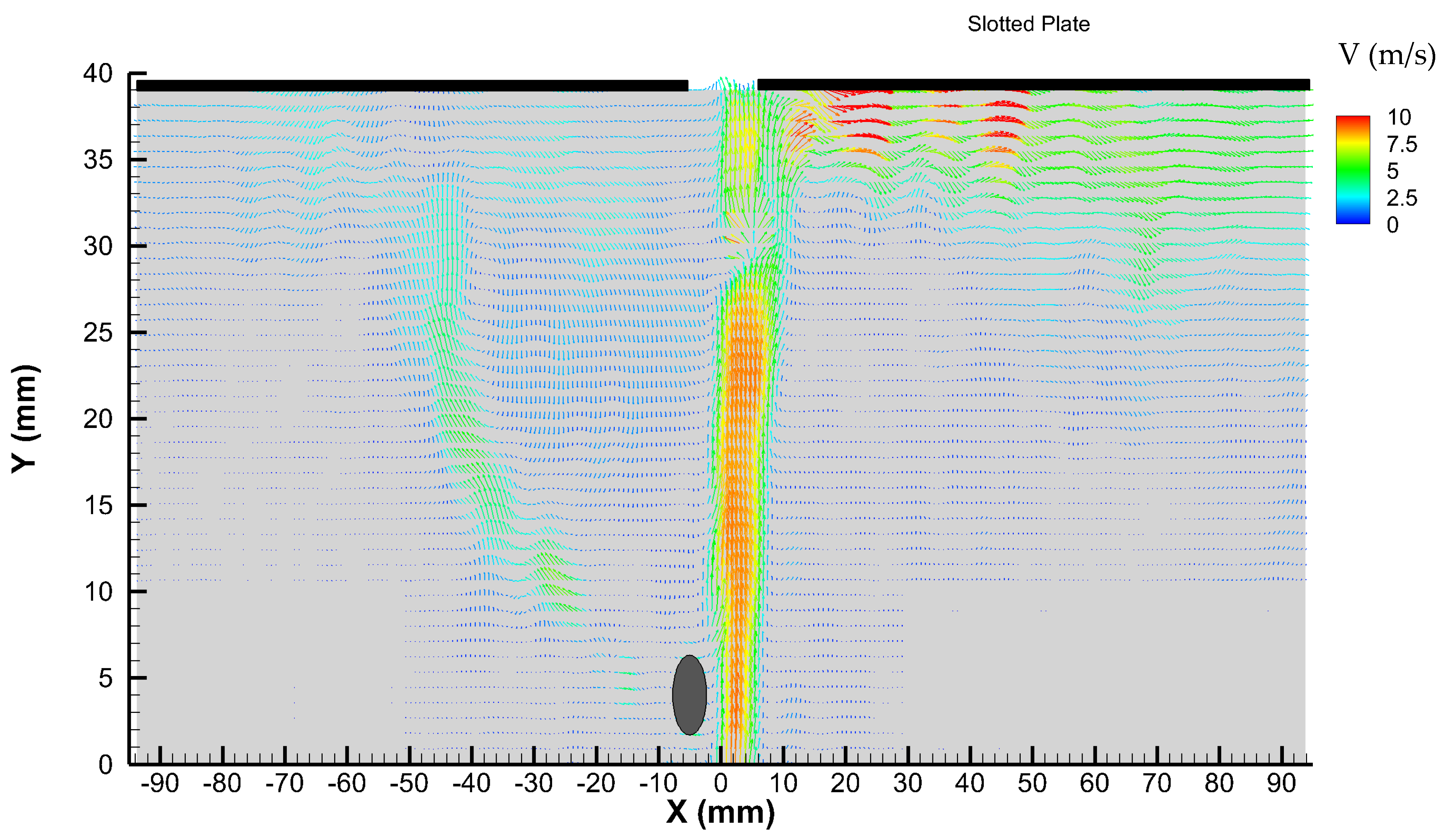
Subsequently, the C-SPIV consists of using two separated and correlated SPIV systems, and adding an inclined mirror to re-illuminate the dark area obscured by the rod’s shadow. The procedure of each SPIV system is the same as the typical one [29]. However, in the common zones, the velocity vector is calculated as the mean velocity obtained by each SPIV measurement. Noting that the difference between the two obtained velocities does not exceed 0.06 m/s. Then, this technique is developed to take measurement in this particular configuration. Instead, if the typical SPIV is applied, the kinematic field in the zone below the rod could not be obtained, which can lead to losing important information about the flow dynamics. In addition, the rod hides the area facing the camera, which limits the calculation of the three-component velocity field in these zones (Figure 3).
where is the pixel size, M is the scale factor of the image, ∆t is the time step between two successive images. As we indicated before, the time Δt is chosen whereby the displacement of the particles between two successive images is between 5 pixels and 10 pixels. In this case, the maximum uncertainty for the three velocity components does not exceed 5%.

Figure 3.
Illustration of hidden areas (gray areas) when the typical SPIV is applied.
3. Results and Discussion
Figure 4 shows the raw images of the upper and lower jet. In the previous work [27], the acoustic measurements indicated the presence of two zones in which the presence of the rod affects the acoustic level. To understand the influence of the presence of this mechanism in each zone on the flow dynamics, the rod is fixed in two positions: (X = −5 mm and Y = 4 mm) and (X = 0 mm and Y = 8 mm), which correspond to the two different zones. The results of the C-SPIV are processed with Matlab, and the kinematic field is presented in Figure 5 and Figure 6 and for the two studied rod positions.
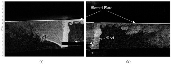
Figure 4.
Raw field on either side of the rod; (a) Lower part of the jet; (b) Upper part of the jet. Re = 5900 and L/H = 4. The rod is located at X = 0 mm and Y = 8 mm.
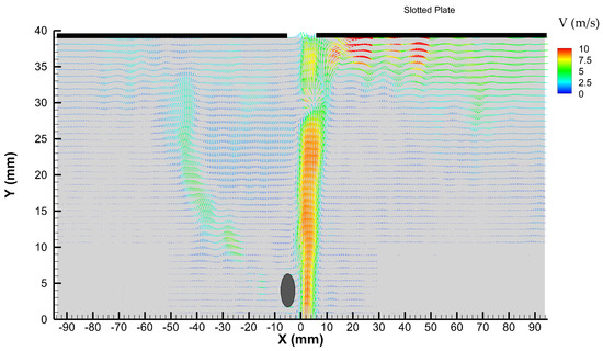
Figure 5.
Visualization of the instantaneous velocity field in the presence of the rod at a time t when the rod occupies the position (X = −5 mm and Y = 4 mm).
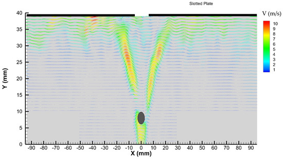
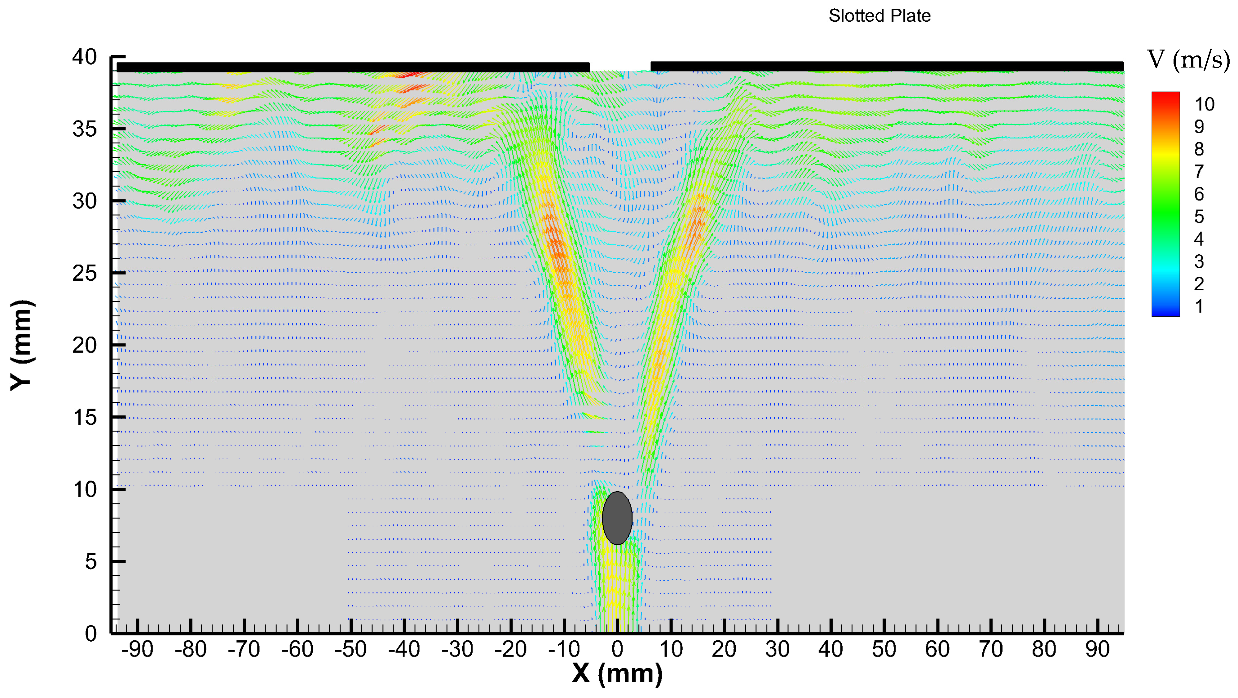
Figure 6.
Visualization of the instantaneous velocity field in the presence of the rod at a time t when the rod occupies the position (X = 0 mm and Y = 8 mm). The circular shape of the rod will appear as an oval shape on the graphs because the scales of the X and Y axes are no longer the same.
To identify the vortical structures, the criterion is calculated for 2-dimensional flow according to [32]:
Noting that, in 2-dimensional flow, the Q and λ2 criteria give the same values with different signs. However, the Graftieaux criteria [30] were not used because they are based on the geometric reading of the flow. Thus, we can detect geometric structures that are well developed but not very energetic. This is why we must combine this type of criterion with an energy detection criterion to have a good identification of vortex structures [33,34]. Examples of the detection of vortices by λ2 criterion are shown in Figure 7.
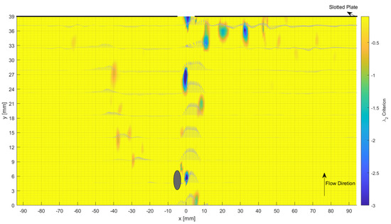
Figure 7.
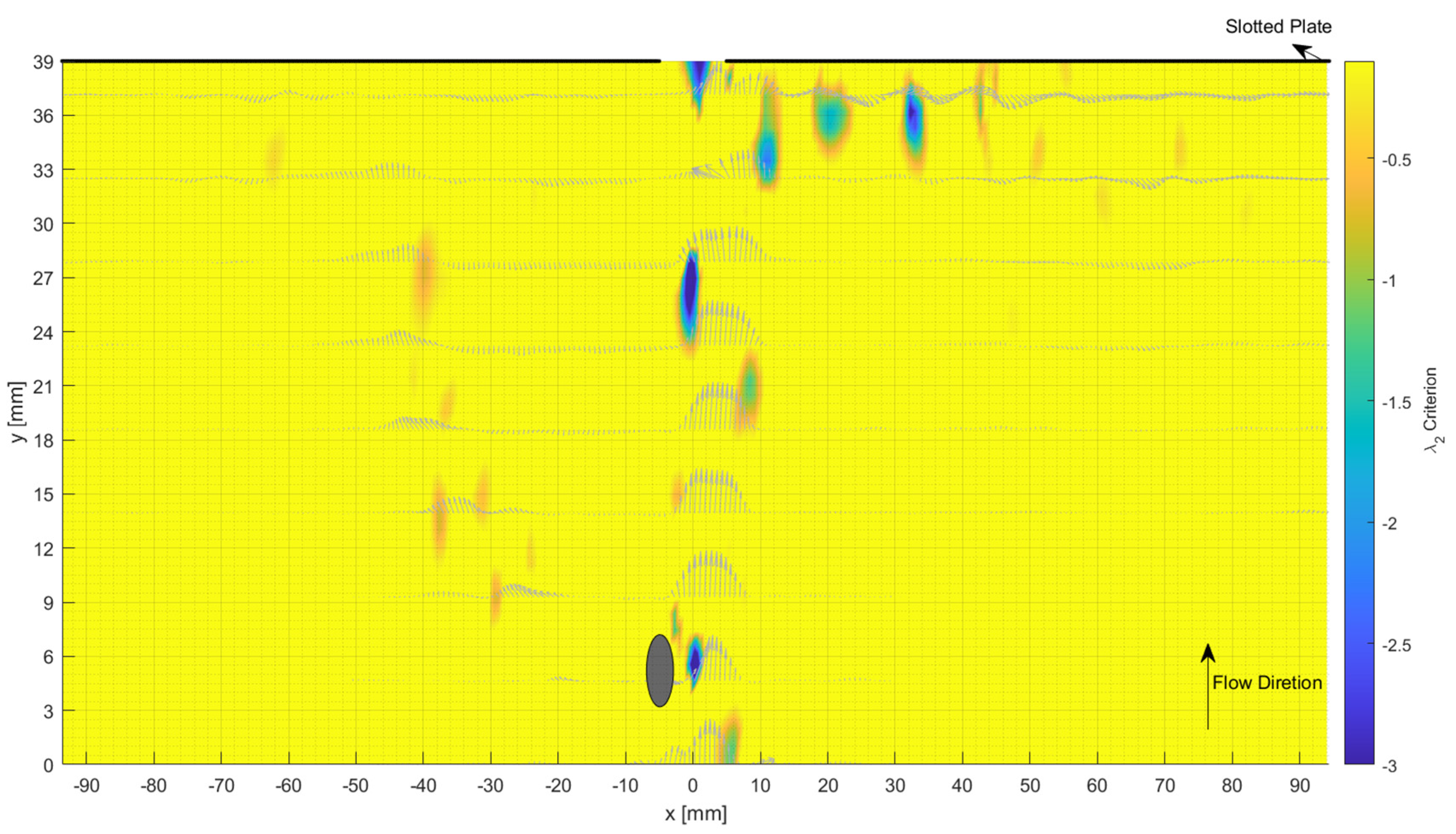
Example of detections of vortex structures by the λ2 criterion, at a time t and when the rod occupies the position (X = −5 mm; Y = 4 mm). The circular shape of the rod will appear as an oval shape on the graphs because the scales of the X and Y axes are no longer the same, and the gray profiles represent the velocity vectors of the flow.
In Figure 7, one can distinguish two paths from the right and the left sides of the rod. The flow of the right is antisymmetric where the presence of the rod delays the formation of the vortices. The flow of the left side, which is far from the axis of the flow, shows small activity which could not be associated to a vortex structure.
The temporal signal of the transverse velocity was extracted from the obtained field at two points where vortices appear to cross: (X = 11 mm; Y = 33 mm) and (X = −31 mm; Y = 15 mm). The spectral analysis of these signals shows that in the presence of the rod, the frequency of the transverse velocity at right and at left is 320 Hz. This is the same frequency obtained for the acoustic sound without the rod.
It is to be noted that, in order to clearly visualize the details of the maps, the scales of the X and Y axes are no longer the same. Consequently, the circular shape of the rod appears in an oval shape on the graph.
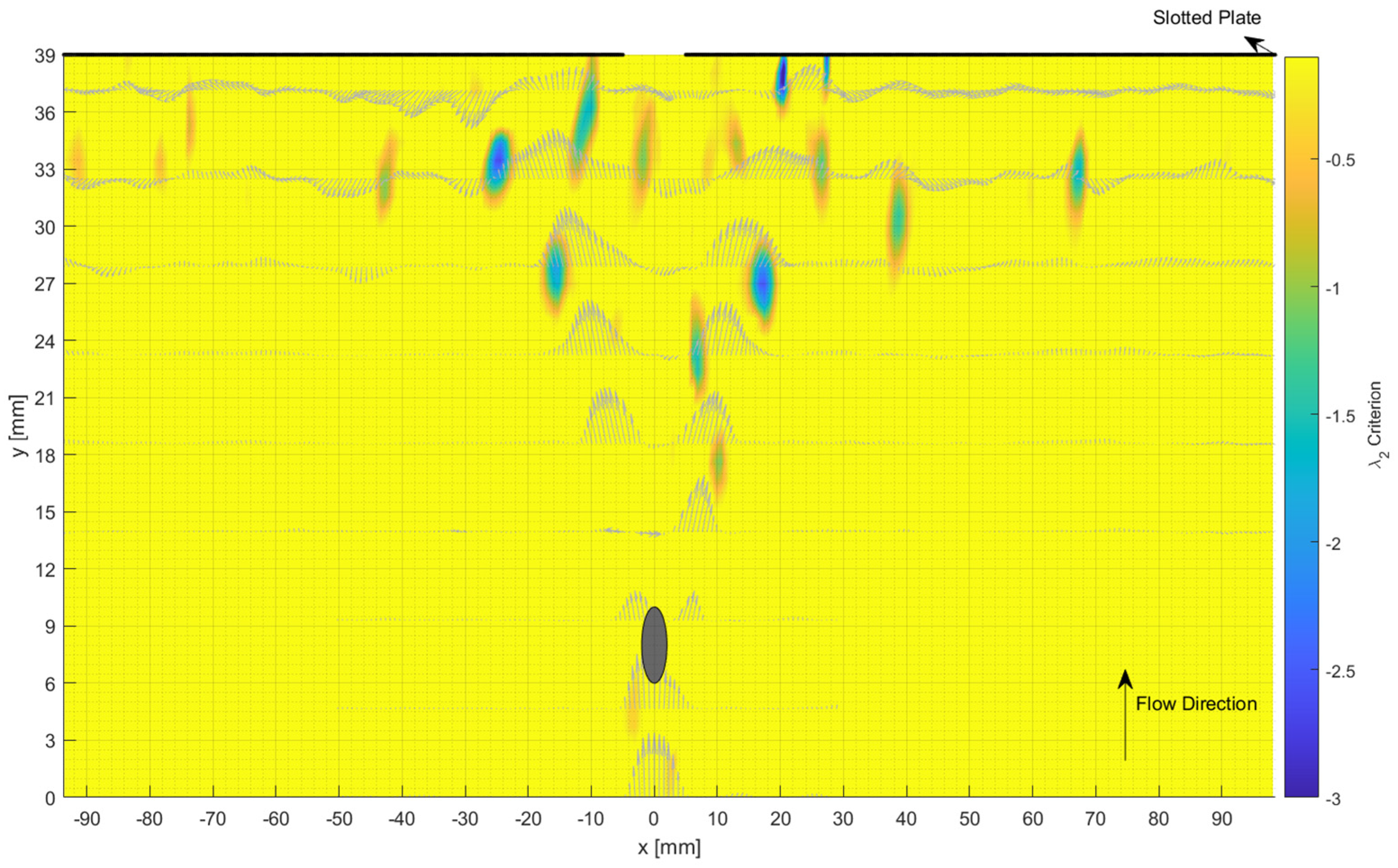
In Figure 8, the vortex structures of the two jets from both sides of the cylinder are almost antisymmetric. The vortex structures respectively coming from the right and the left sides hit the wall of the plate on the sides of the slot creating two zones of recirculation on either side of the slot. Furthermore, we extracted the temporal signal of the transverse velocities at two points (X = 18.5 mm; Y = 27 mm) and (X = −18.5 mm; Y = 27 mm). The spectra of these two signals show a same frequency of 326 Hz. This is slightly different from frequency obtained for acoustic sound without the rod (320 Hz).
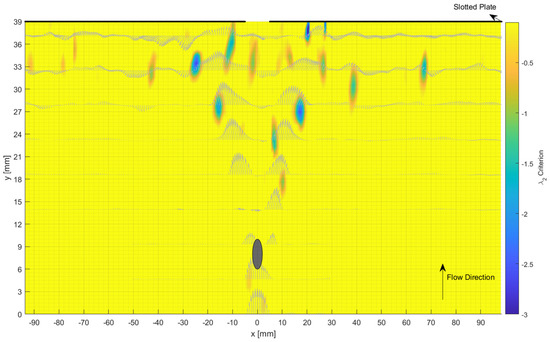
Figure 8.
Example of detections of vortex structures by the criterion λ2, at a time t and when the rod occupies the position (X = 0 mm; Y = 8 mm). The circular shape of the rod will appear in an oval shape on the graphs because the scales of the X and Y axes are no longer the same and the gray profiles represent the velocity vectors of the flow.
As it was shown in [22], the self-sustained tones occur in very specific conditions of phase allowing optimal transfer of energy from the kinematic field of the jet to the acoustic one. The introduction of the rod into the dynamic field modifies the energy transfer conditions and thus may destroy the self-sustaining sound loops. Thus, we investigated the relationships between the turbulent kinetic energy and the acoustic field for this Reynolds number Re = 5900. In this paper we consider the case without rod and with rod (of diameter 4 mm).
The surface density of the instantaneous and normalized mean turbulent kinetic energy TKE (t) was calculated, at each instant, and averaged over the entire control zone as follows:
where , , and are respectively the fluctuating velocities in X, Y, and Z directions at the point (i, j) at the instant t. is the average velocity at the jet exit.
From the C-SPIV measurements, the area density of the instantaneous mean turbulent kinetic energy TKE (t) was calculated over the area as shown in Figure 8.
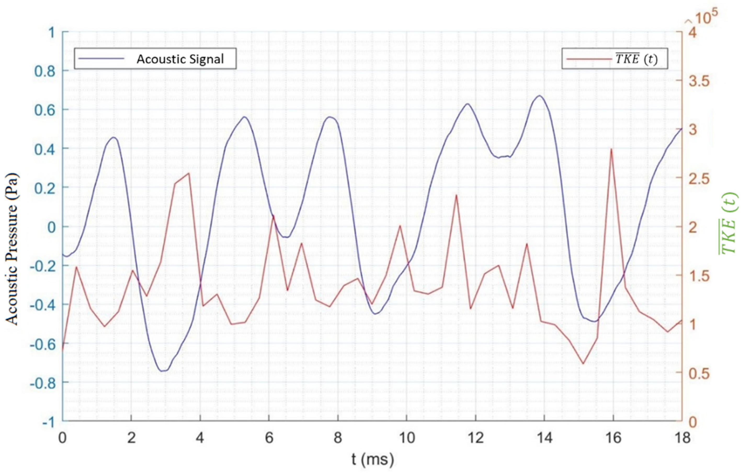
Figure 9 shows the temporal variation of the sound pressure (curve in blue) as well as TKE (t) (curve in red) over a time interval of 18 ms. These two quantities were sampled at 15,000 Hz and 2500 Hz respectively. We can notice that the relative minima of the acoustic signal correspond, with a slight shift in time, to the relative maxima of TKE (t) and the relative maxima of the acoustic signal are slightly shifted in time with the relative minima of TKE (t). This result could suggest that when the energy transfer is optimal, the sound pressure of the radiated field is maximum while the turbulent energy is minimum with a slight phase shift [20].
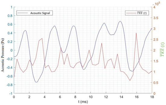
Figure 9.
Evolution of TKE (t) (in red) and the sound pressure signal (in blue). Reynolds number Re = 5900 and L/H = 4. Without a rod.
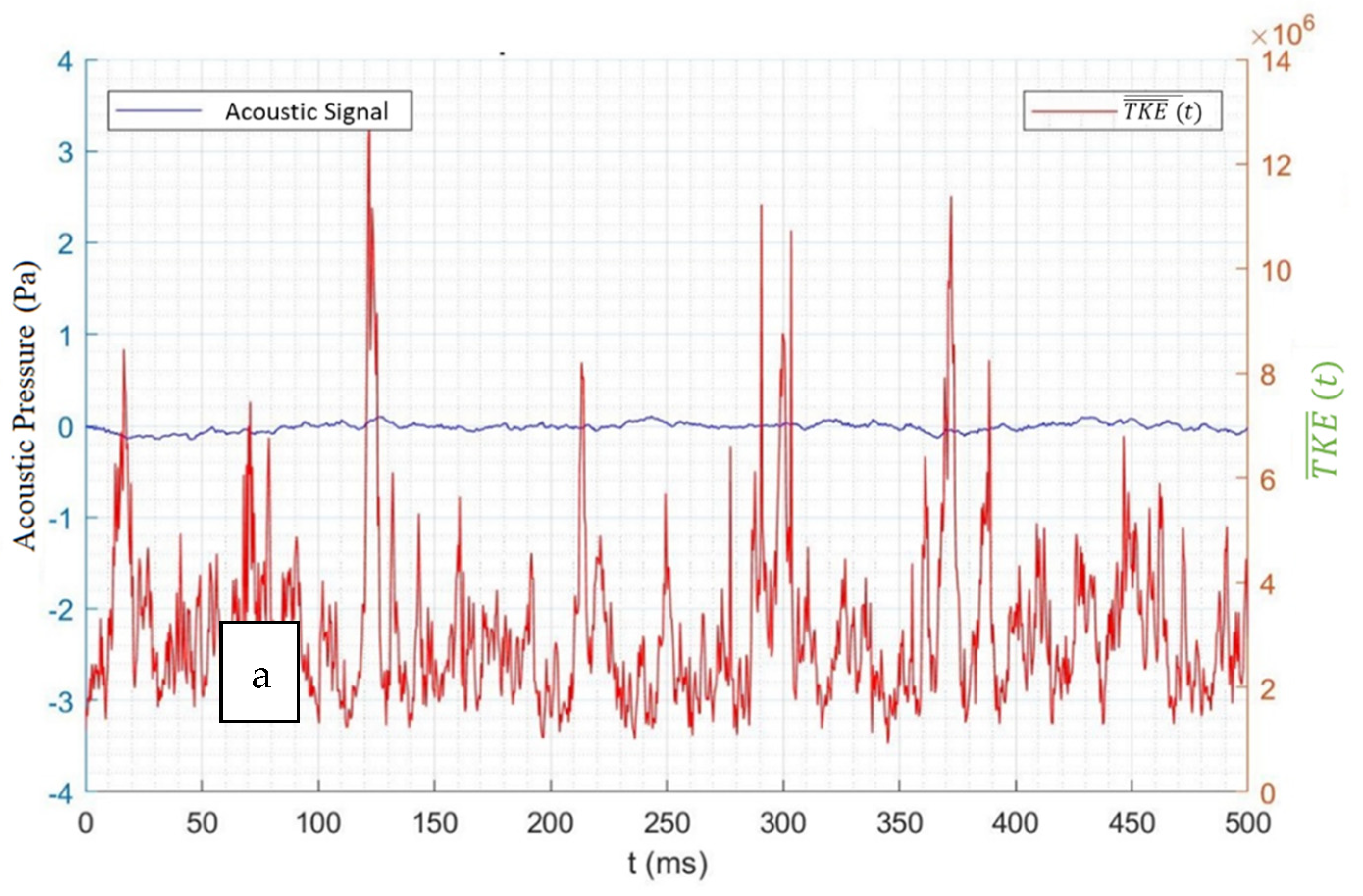
In Figure 10a,b, the temporal variation of the sound pressure (curve in blue) as well as TKE (t) (curve in red) are presented over a time interval of 500 ms. These two quantities were sampled at 15,000 Hz and 2500 Hz respectively. One can see that these curves show no periodicity and present a random character in their evolution. This could confirm that the presence of the rod, despite the presence of very high turbulent energy, destroyed the energy transfer conditions between the turbulent kinetic energy and the radiated sound fields since the acoustic signal is very weak. In Figure 10b one can notice that the TKE (t) is of the same order of magnitude as in the case where the rod is not installed.
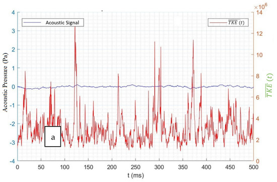
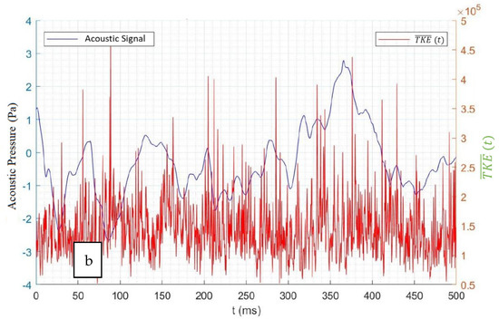
Figure 10.
Evolution of TKE (t) (in red) and the sound pressure signal (in blue). Reynolds number Re = 5900 and L/H = 4. (a) rod located at (X = 0 mm; Y = 8 mm), (b) rod located at (X = −5 mm; Y = 4 mm).
4. Conclusions
In this paper, a combined SPIV (C-SPIV) technique was proposed to overcome experimental difficulties when taking SPIV images in the presence of an obstacle, which can be used to control the noise generation because of its shadow. In the present paper, the velocity field of the jet flow around the rod is obtained using the C-SPIV technique. It was shown that this method presents a great advantage as compared to the traditional SPIV. In terms of flow analysis, it has been shown that the presence of the rod divided the flow into two streams. The investigation of the TKE and acoustic signal showed that when the rod is introduced, the acoustic signal becomes very weak despite the high TKE amplitudes. This could reveal that the presence of the rod has unstructured the energy transfers from the dynamic field to the acoustic one.
Future work would focus on the flow dynamics at different positions occupied by the rod using the C-SPIV measurement. Thus, all positions between the plate and the nozzle should be considered to identify optimal positions for acoustic control. Model reduction technique such as the proper orthogonal decomposition (POD) and the dynamic mode decomposition (DMD) are also to be investigated on such flows. This would allow us to detect dominant structures of the flow which could be responsible of the acoustic generation.
Author Contributions
Conceptualization, A.S., M.A., K.A.M. and H.H.A.; methodology, A.S., M.A., K.A.M. and H.H.A.; software, M.A.; writing—original draft preparation, N.E.A., H.H.A. and M.E.H.; writing—review and editing, N.E.A., H.H.A. and M.E.H.; project administration, A.S., K.A.M. and H.H.A.; funding acquisition, A.S. All authors have read and agreed to the published version of the manuscript.
Funding
This research received no external funding.
Acknowledgments
The authors wish to thank FEDER and the region of Nouvelle Aquitaine, France for its financial support.
Conflicts of Interest
The authors declare no conflict of interest.
References
- Valentich, G.M. Flow Field and Acoustic Characterization of Non-Axisymmetric Jets. Ph.D. Thesis, Florida State University, Tallahassee, FL, USA, 2016. [Google Scholar]
- Hamdi, J.; Assoum, H.H.; Alkheir, M.; Abed-Meraïm, K.; Cauet, S.; Sakout, A. Analysis of the 3D flow of an impinging jet on a slotted plate using TR-Tomo PIV and Proper Orthogonal Decomposition. Energy Rep. 2020, 6, 158–163. [Google Scholar] [CrossRef]
- Mrach, T.; Alkheir, M.; El Hassan, M.; Assoum, H.H.; Etien, E.; Abed-Meraim, K. Experimental study of the thermal effect on the acoustic field generated by a jet impinging on a slotted heated plate. Energy Rep. 2020, 6, 497–501. [Google Scholar] [CrossRef]
- Hamdi, J.; Assoum, H.; Abed-Meraïm, K.; Sakout, A. Analysis of the effect of the 3C kinematic field of a confined impinging jet on a slotted plate by stereoscopic PIV. Eur. J. Mech.-BFluids 2019, 76, 243–258. [Google Scholar] [CrossRef]
- Hamdi, J.; Assoum, H.; Abed-Meraïm, K.; Sakout, A. Volume reconstruction of an impinging jet obtained from stereoscopic-PIV data using POD. Eur. J. Mech.-BFluids 2018, 67, 433–445. [Google Scholar] [CrossRef]
- El Hassan, M.; Bukharin, N.; Al-Kouz, W.; Zhang, J.-W.; Li, W.-F. A Review on the Erosion Mechanism in Cavitating Jets and Their Industrial Applications. Appl. Sci. 2021, 11, 3166. [Google Scholar] [CrossRef]
- Bukharin, N.; El Hassan, M.; Omelyanyuk, M.; Nobes, D. Applications of cavitating jets to radioactive scale cleaning in pipes. Energy Rep. 2020, 6, 1237–1243. [Google Scholar] [CrossRef]
- El Hassan, M.; Assoum, H.H.; Martinuzzi, R.; Sobolik, V.; Abed-Meraim, K.; Sakout, A. Experimental investigation of the wall shear stress in a circular impinging jet. Phys. Fluids 2013, 25, 077101. [Google Scholar] [CrossRef]
- El Hassan, M.; Meslem, A. Time-resolved stereoscopic particle image velocimetry investigation of the entrainment in the near field of circular and daisy-shaped orifice jets. Phys. Fluids 2010, 22, 035107. [Google Scholar] [CrossRef]
- Namer, I.; Ötügen, M.V. Velocity measurements in a plane turbulent air jet at moderate Reynolds numbers. Exp. Fluids 1988, 6, 387–399. [Google Scholar] [CrossRef]
- Adrian, R.J. Twenty years of particle image velocimetry. Exp. Fluids 2005, 39, 159–169. [Google Scholar] [CrossRef]
- Willert, C.E.; Gharib, M. Digital particle image velocimetry. Exp. Fluids 1991, 10, 181–193. [Google Scholar] [CrossRef]
- McKenna, S.P.; McGillis, W.R. Performance of digital image velocimetry processing techniques. Exp. Fluids 2002, 32, 106–115. [Google Scholar] [CrossRef]
- Rockwell, D.; Magness, C.; Towfighi, J.; Akin, O.; Corcoran, T. High image-density particle image velocimetry using laser scanning techniques. Exp. Fluids 1993, 14, 181–192. [Google Scholar] [CrossRef]
- Zhang, Y. Experimental studies of the turbulence structures of impinging reacting jets using time-resolved particle image velocimetry visualisation, hot wire anemometry and acoustic signal processing. Exp. Fluids 2000, 29, S282–S290. [Google Scholar] [CrossRef]
- Assoum, H.H.; Hamdi, J.; Abed-Meraïm, K.; El Hassan, M.; Hammoud, A.; Sakout, A. Experimental investigation the turbulent kinetic energy and the acoustic field in a rectangular jet impinging a slotted plate. Energy Procedia 2017, 139, 398–403. [Google Scholar] [CrossRef]
- Assoum, H.H.; Hamdi, J.; Abed-Meraïm, K.; El Hassan, M.; Ali, M.; Sakout, A. Correlation between the acoustic field and the transverse velocity in a plane impinging jet in the presence of self-sustaining tones. Energy Procedia 2017, 139, 391–397. [Google Scholar] [CrossRef]
- Prasad, A.K. Stereoscopic particle image velocimetry. Exp. Fluids 2000, 29, 103–116. [Google Scholar] [CrossRef]
- Shi, S.; Ding, J.; Atkinson, C.; Soria, J.; New, T.H. A detailed comparison of single-camera light-field PIV and tomographic PIV. Exp. Fluids 2018, 59, 46. [Google Scholar] [CrossRef]
- Assoum, H.H.; El Hassan, M.; Hamdi, J.; Alkheir, M.; Meraim, K.A.; Sakout, A. Turbulent Kinetic Energy and self-sustaining tones in an impinging jet using High Speed 3D Tomographic-PIV. Energy Rep. 2020, 6, 802–806. [Google Scholar] [CrossRef]
- Mullin, J.A.; Dahm, W.J.A. Dual-plane stereo particle image velocimetry (DSPIV) for measuring velocity gradient fields at intermediate and small scales of turbulent flows. Exp. Fluids 2005, 38, 185–196. [Google Scholar] [CrossRef] [Green Version]
- Assoum, H.H.; Hamdi, J.; El Hassan, M.; Abed-Meraim, K.; El Kheir, M.; Mrach, T.; El Asmar, S.; Sakout, A. Turbulent kinetic energy and self-sustaining tones: Experimental study of a rectangular impinging jet using high Speed 3D tomographic Particle Image Velocimetry. J. Mech. Eng. Sci. 2020, 14, 6322–6333. [Google Scholar] [CrossRef] [Green Version]
- Assoum, H.H.; Hamdi, J.; El Hassan, M.; Mrach, T.; Abed Meraim, K.; Sakout, A. Energy transfers between aerodynamic and acoustic fields in a rectangular impinging jet. Energy Rep. 2020, 6, 812–816. [Google Scholar] [CrossRef]
- Assoum, H.; Hamdi, J.; Abed-Meraïm, K.; Al Kheir, M.; Mrach, T.; El Soufi, L.; Sakout, A. Spatio-Temporal Changes in the Turbulent Kinetic Energy of a Rectangular Jet Impinging on a Slotted Plate Analyzed with High Speed 3D Tomographic-Particle Image Velocimetry. Int. J. Heat Technol. 2019, 37, 1071–1079. [Google Scholar] [CrossRef] [Green Version]
- Assoum, H.H.; El Hassan, M.; Abed-Meraim, K.; Sakout, A. The vortex dynamics and the self sustained tones in a plane jet impinging on a slotted plate. Eur. J. Mech.-BFluids 2014, 48, 231–235. [Google Scholar] [CrossRef]
- Assoum, H.H.; Hassan, M.E.; Abed-Meraïm, K.; Martinuzzi, R.; Sakout, A. Experimental analysis of the aero-acoustic coupling in a plane impinging jet on a slotted plate. Fluid Dyn. Res. 2013, 45, 045503. [Google Scholar] [CrossRef]
- Alkheir, M.; Mrach, T.; Hamdi, J.; Abed-Meraim, K.; Rambault, L.; El Hassan, M. Effect of passive control cylinder on the acoustic generation of a rectangular impinging jet on a slotted plate. Energy Rep. 2020, 6, 549–553. [Google Scholar] [CrossRef]
- Phantom v710 Datasheet. Available online: https://w3.pppl.gov/~szweben/Cmod%20guide/v710.pdf (accessed on 14 June 2021).
- Raffel, M.; Willert, C.; Scarano, F.; Kähler, C.; Wereley, S. Particle Image Velocimetry: A Practical Guide; Springer International Publishing: Cham, Switzerland, 2018. [Google Scholar]
- Graftieaux, L.; Michard, M.; Grosjean, N. Combining PIV, POD and vortex identification algorithms for the study of unsteady turbulent swirling flows. Meas. Sci. Technol. 2001, 12, 1422–1429. [Google Scholar] [CrossRef]
- Keane, R.D.; Adrian, R.J. Theory of cross-correlation analysis of PIV images. Appl. Sci. Res. 1992, 49, 191–215. [Google Scholar] [CrossRef]
- Fiabane, L. Méthodes Analytiques de Caractérisation des Structures Cohérentes Contribuant aux Efforts Aérodynamiques. Ph.D. Thesis, Ecole Polytechnique X, Palaiseau, France, 2010. [Google Scholar]
- Kolář, V. Vortex identification: New requirements and limitations. Int. J. Heat Fluid Flow 2007, 28, 638–652. [Google Scholar] [CrossRef]
- Jeong, J.; Hussain, F.; Schoppa, W.; Kim, J. Coherent structures near the wall in a turbulent channel flow. J. Fluid Mech. 1997, 332, 185–214. [Google Scholar] [CrossRef] [Green Version]


Publisher’s Note: MDPI stays neutral with regard to jurisdictional claims in published maps and institutional affiliations. |
© 2021 by the authors. Licensee MDPI, Basel, Switzerland. This article is an open access article distributed under the terms and conditions of the Creative Commons Attribution (CC BY) license (https://creativecommons.org/licenses/by/4.0/).