On Mixed Convection in a Horizontal Channel, Viscous Dissipation and Flow Duality

Abstract

The conditions defining a stationary fluid flow may lead to a multiplicity of solutions. This circumstance is widely documented in the literature when mixed convection in a vertical channel or duct is accompanied by an important effect of viscous dissipation. Usually, there are double stationary solutions with a parallel velocity field which satisfy given temperature boundary conditions and with a prescribed mass flow rate. However, in a vertical internal flow, the dual solutions can be determined only numerically as they do not have a closed analytical form. This study shows that, in a horizontal channel, stationary mixed convection with viscous dissipation shows up dual flow branches whose mathematical expressions can be determined analytically. The features of these dual flows are discussed.

1. Introduction

There exists a wide literature pointing out that the governing equations of fluid flow may allow multiple solutions for a given properly conditioned problem. In fact, it is widely assumed that the stationary and fully developed flow of a fluid in a duct or channel with assigned wall conditions for the temperature and for the velocity (typically no slip) is unique provided that a given mass flow rate or pressure gradient is prescribed. This is the case of some elementary solutions for isothermal flow available in all textbooks of fluid dynamics, such as the Poiseuille flow or the Poiseuille–Couette flow, as well as for less known solutions relative to natural or mixed convection heat transfer, such as the Batchelor’s profile [1]. However, this widely assumed behaviour is not a general feature of stationary fully–developed internal flows. Significant counterexamples exist when the nonlinear nature of the governing equations for fluid flow emerges in the stationary fully–developed regime. There are typical conditions leading to such a situation; one is the non–negligible viscous dissipation effect in a buoyant flow. There are well–documented case studies of this type addressing situations where steady natural or mixed convection dual flows arise in vertical channels or ducts [2,3,4,5,6,7]. A general feature of such solutions is that they are not expressed in a closed analytical form, but they are obtained by numerical methods, usually the shooting method implemented, for example via a Runge–Kutta solver or a power–series technique yielding a recursive determination of the series coefficients.

The analysis of viscous dissipation effects in forced convection and mixed convection flows has a significant impact for both engineering and geophysical applications. Engineering applications are oriented to the analysis and the design of the thermal treatment of fluids, important to the food processing industry and to the chemical engineering analysis of organic and/or polymeric fluid flows. Geophysical applications are devised as typical of the interplay between buoyancy and viscous dissipation effects, as pointed out in the classical papers by Gebhart [8] and by Gebhart and Mollendorf [9]. These authors introduced the dissipation parameter (now widely known as the Gebhart number) as the key parameter governing the phenomenon.

The aim of this paper is to examine the stationary mixed convection flow with viscous dissipation in a horizontal channel, where the channel boundary walls are adiabatic and the velocity field is parallel. It will be shown that there exist dual solutions for every possible assignment of the mass flow rate, expressed in non–dimensional terms through the Péclet number. The striking feature of this flow problem is that the dual solutions are expressed in a closed form as polynomials in the transverse coordinate. This paper mirrors an analogous study carried out for a fluid saturated porous medium governed by Darcy’s law [10]. The novel feature of the investigation presented here is that a Newtonian fluid flow is considered instead of the seepage flow in a porous medium.

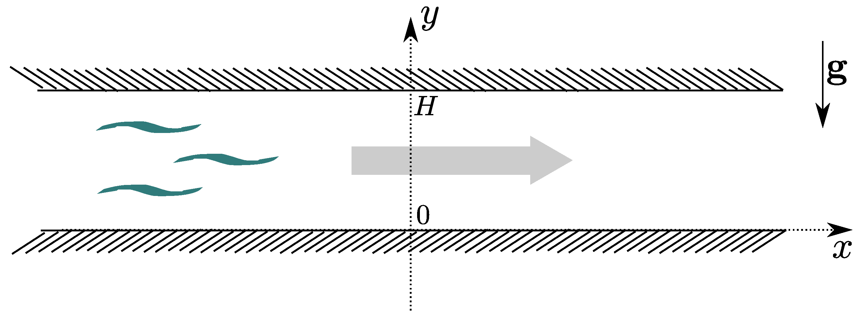
2. Governing Equations

Let us consider a horizontal channel bounded by rigid walls at $y=0,H$. The y axis is vertical, while the $(x,z)$ axes are horizontal. As shown in Figure 1, the gravitational acceleration is $\mathbf{g}=-g{\widehat{\mathbf{e}}}_y$, where ${\widehat{\mathbf{e}}}_y$ is the unit vector along the y axis. The rigid boundary walls are modelled as perfectly adiabatic.

We assume the validity of the Boussinesq approximation and we assume the effect of viscous dissipation as non–negligible. Thus, a dimensionless formulation of the local mass, momentum and energy balance equations for a Newtonian fluid flowing in the channel can be expressed as [8,9]

$$\mathbf{\nabla }·\mathbf{u}=0,$$

(1)

$$\frac{1}{Pr}\left[\frac{\partial \mathbf{u}}{\partial t}+(\mathbf{u}·\mathbf{\nabla })\mathbf{u}\right]=-\mathbf{\nabla }p+T{\widehat{\mathbf{e}}}_y+{\mathrm{\nabla }}^2\mathbf{u},$$

(2)

$$\frac{\partial T}{\partial t}+(\mathbf{u}·\mathbf{\nabla })T={\mathrm{\nabla }}^{2}T+\mathrm{Ge}\mathrm{\Phi }.$$

(3)

In Equation (3), $\mathrm{\Phi }$ denotes the dissipation function,

$$\begin{array}{c}\mathrm{\Phi }=\frac{\partial u_i}{\partial x_j}\frac{\partial u_i}{\partial x_j}+\frac{\partial u_i}{\partial x_j}\frac{\partial u_j}{\partial x_i},\end{array}$$

(4)

where $u_i$ and $x_i$ are the ith Cartesian components of the velocity vector and of the position vector, respectively, while repeated indices i and j are implicitly summed over.

The dimensionless boundary conditions are formulated as

$$\begin{array}{c}\mathbf{u}=0,\frac{\partial T}{\partial y}=0\mathrm{for}y=0,1.\end{array}$$

(5)

The scaling adopted for the dimensional quantities in order to obtain Equations (1)–(3) and (5) is given by

$$\begin{array}{c}\frac{\mathbf{x}}{H}={\mathbf{x}}_{nd},\frac{t}{H^2/\alpha }=t_{nd},\frac{\mathbf{u}}{\alpha /H}={\mathbf{u}}_{nd},\frac{p}{\rho \alpha \nu /H^2}=p_{nd}\\ \frac{T-T_0}{\Delta T}=T_{nd},\frac{\mathrm{\Phi }}{{\alpha }^2/H^4}={\mathrm{\Phi }}_{nd},\end{array}$$

(6)

where the subscript “$nd$” denotes the dimensionless quantities. In Equations (1)–(3) and in the forthcoming equations, such a subscript is omitted for the sake of simplicity. Most of our study, starting from Equation (8), involves dimensionless quantities and, when some dimensional field or quantity is used, this will be explicitly stated to avoid any confusion.

In Equation (6), $\Delta T=\alpha \nu /\left(g\beta H^3\right)$ and $T_0$ is the reference temperature employed to evaluate the fluid properties within the Boussinesq approximation. The Prandtl and Gebhart numbers are defined as

$$\begin{array}{c}Pr=\frac{\nu }{\alpha },\mathrm{Ge}=\frac{g\beta H}{c}.\end{array}$$

(7)

In Equations (1)–(7), $\mathbf{u}$ is the velocity, p is the dynamic pressure, i.e., the local difference between the pressure and the hydrostatic pressure, T is the temperature, and t is time. Furthermore, $\alpha$ is the thermal diffusivity, $\nu$ is the kinematic viscosity, $\beta$ is the thermal expansion coefficient, $\rho$ is the constant reference density and c is the specific heat.

We said that the scaling defined by Equation (6) involves the reference temperature $T_0$. The reliability of the model based on the Boussinesq approximation greatly depends on the choice of $T_0$. The optimal choice is one that minimises the error in the substitution of the variable density with its reference value. Such a choice of $T_0$ is the average value over the spatial domain where the flow is studied [11]. The dimensionless spatial region where the flow solution is to be determined can be defined, in terms of $(x,y,z)$, as the Cartesian product $[-a,a]\times [0,1]\times [-b,b]$ where the geometric aspect ratios a and b are chosen arbitrarily at this stage. In its dimensionless formulation, the choice of the reference temperature is expressed by the constraint

$$\begin{array}{c}\underset{-a}{\overset{a}{\int }}\mathrm{d}x\underset{0}{\overset{1}{\int }}\mathrm{d}y\underset{-b}{\overset{b}{\int }}\mathrm{d}zT=0,\end{array}$$

(8)

to be satisfied by the dimensionless temperature T.

3. Flow Duality

Equations (1)–(3) and (5) admit stationary two–dimensional solutions, where the velocity field $\mathbf{u}=(u,v,0)$, the dynamic pressure field p and the temperature field T depend only on the coordinates $(x,y)$. Among such solutions, we seek those satisfying the requirement

$$\begin{array}{c}u=\mathrm{Pe}F\left(y\right),v=0,\end{array}$$

(9)

where $F\left(y\right)$ is a function satisfying an integral normalisation condition,

$$\begin{array}{c}\underset{0}{\overset{1}{\int }}F\left(y\right)\mathrm{d}y=1,\end{array}$$

(10)

so that the Péclet number, $\mathrm{Pe}$, expresses the dimensionless average velocity along the x direction. In other words, if we denote by $U_0$ the dimensional average velocity in a $x=constant$ cross–section, we can write

$$\begin{array}{c}\mathrm{Pe}=\frac{U_{0}H}{\alpha },\end{array}$$

(11)

since $\alpha /H$ is the velocity scale employed in Equation (6).

3.1. The Velocity Field and the Temperature Field

Equation (9) identically satisfies Equation (1), while Equations (2) and (3) are drastically simplified to

$$-\frac{\partial p}{\partial x}+\mathrm{Pe}\frac{{\mathrm{d}}^{2}F\left(y\right)}{\mathrm{d}{y}^2}=0,$$

(12)

$$-\frac{\partial p}{\partial y}+T=0,$$

(13)

$$\mathrm{Pe}F\left(y\right)\frac{\partial T}{\partial x}=\frac{{\partial }^{2}T}{\partial x}+\frac{{\partial }^{2}T}{\partial y}+\mathrm{Ge}\mathrm{\Phi },$$

(14)

where, on account of Equations (4) and (9), the dissipation function $\mathrm{\Phi }$ is given by

$$\begin{array}{c}\mathrm{\Phi }={\mathrm{Pe}}^2{\left[\frac{\mathrm{d}F\left(y\right)}{\mathrm{d}y}\right]}^2.\end{array}$$

(15)

We now derive Equation (12) with respect to y, we derive Equation (13) with respect to x and subtract the two resulting equations so that the mixed second–order partial derivatives of p cancel out. Thus, we obtain

$$\begin{array}{c}\frac{\partial T}{\partial x}=\mathrm{Pe}\frac{{\mathrm{d}}^{3}F\left(y\right)}{\mathrm{d}{y}^3}.\end{array}$$

(16)

On account of Equation (9), the boundary conditions (5) yield

$$\begin{array}{c}F\left(0\right)=0=F\left(1\right).\end{array}$$

(17)

Let us derive Equation (14) with respect to x by taking into account that, from Equation (15), $\mathrm{\Phi }$ depends only on y. Thus, we have

$$\begin{array}{c}\mathrm{Pe}F\left(y\right)\frac{{\partial }^{2}T}{\partial x^2}=\frac{{\partial }^{3}T}{\partial x^3}+\frac{{\partial }^2}{\partial y^2}\frac{\partial T}{\partial x}.\end{array}$$

(18)

Equation (16) implies that $\partial T/\partial x$ depends only on y, so that both ${\partial }^{2}T/\partial x^2$ and ${\partial }^{3}T/\partial x^3$ are identically zero. Therefore, the substitution of Equation (16) into Equation (18) yields

$$\begin{array}{c}\frac{{\mathrm{d}}^{5}F\left(y\right)}{\mathrm{d}{y}^5}=0.\end{array}$$

(19)

Thus, we can conclude that $F\left(y\right)$ is a fourth degree polynomial in y.

$$\begin{array}{c}F\left(y\right)=c_0+c_{1}y+c_2{y}^2+c_3{y}^3+c_4{y}^4,\end{array}$$

(20)

where $c_0$, $c_1$, $c_2$, $c_3$ and $c_4$ are constants. By using Equations (10) and (17), we obtain

$$\begin{array}{c}{c}_0=0,c_1+c_2+c_3+c_4=0,\frac{1}{2}{c}_1+\frac{1}{3}{c}_2+\frac{1}{4}{c}_3+\frac{1}{5}{c}_4=1.\end{array}$$

(21)

The general solution of Equation (16) can be written as

$$\begin{array}{c}T=\mathrm{Pe}\frac{{\mathrm{d}}^{3}F\left(y\right)}{\mathrm{d}{y}^3}x+{\mathrm{Pe}}^{2}G\left(y\right)=6\mathrm{Pe}(c_3+4c_{4}y)x+{\mathrm{Pe}}^{2}G\left(y\right),\end{array}$$

(22)

where $G\left(y\right)$ is a function to be determined, and Equation (20) has been employed.

On account of Equation (22), the boundary conditions (5) yield

$$\begin{array}{c}\mathrm{Pe}\frac{\mathrm{d}G\left(y\right)}{\mathrm{d}y}{{|}_{y=0}+24c_{4}x=0,\mathrm{Pe}\frac{\mathrm{d}G\left(y\right)}{\mathrm{d}y}|}_{y=1}+24c_{4}x=0,\end{array}$$

(23)

which can be satisfied for every x if and only if

$$\begin{array}{c}\frac{\mathrm{d}G\left(y\right)}{\mathrm{d}y}{|}_{y=0}=0={\frac{\mathrm{d}G\left(y\right)}{\mathrm{d}y}|}_{y=1},c_4=0.\end{array}$$

(24)

Then, Equation (21) yields

$$\begin{array}{c}\left\{\begin{array}{c}{c}_1+c_2+c_3=0\hfill \\ 6c_1+4c_2+3c_3=12\hfill \end{array}\right.⟹\left\{\begin{array}{c}{c}_2=-3c_1+12\hfill \\ c_3=2c_1-12\hfill \end{array}\right.\end{array}$$

(25)

We can rewrite Equations (20) and (22) as

$$\begin{array}{c}F\left(y\right)=c_{1}y-3(c_1-4)y^2+2(c_1-6)y^3,\\ T=12\mathrm{Pe}(c_1-6)x+{\mathrm{Pe}}^{2}G\left(y\right).\end{array}$$

(26)

The integral constraint (8) is satisfied, when T is expressed by Equation (26), if $G\left(y\right)$ has a zero average value,

$$\begin{array}{c}\underset{0}{\overset{1}{\int }}G\left(y\right)\mathrm{d}y=0.\end{array}$$

(27)

By substituting Equations (15), (16) and (26) into Equation (14), we obtain

$$\begin{array}{c}F\left(y\right)\frac{{\mathrm{d}}^{3}F\left(y\right)}{\mathrm{d}{y}^3}=\frac{{\mathrm{d}}^{2}G\left(y\right)}{\mathrm{d}{y}^2}+\mathrm{Ge}{\left[\frac{\mathrm{d}F\left(y\right)}{\mathrm{d}y}\right]}^2.\end{array}$$

(28)

By employing the expression of $F\left(y\right)$ given by Equation (26), we can reformulate Equation (28) as

$$\begin{array}{c}\frac{{\mathrm{d}}^{2}G\left(y\right)}{\mathrm{d}{y}^2}=-36\mathrm{Ge}{(c_1-6)}^2{y}^4+24(c_1-6)\left[3(c_1-4)\mathrm{Ge}+c_1-6\right]y^3\\ +12\left[30c_1(\mathrm{Ge}+1)-24(2\mathrm{Ge}+3)-c_1^2(4\mathrm{Ge}+3)\right]y^2\\ +12c_1\left[c_1-6+(c_1-4)\mathrm{Ge}\right]y-c_1^2\mathrm{Ge}.\end{array}$$

(29)

An integration of Equation (29) yields

$$\begin{array}{c}\frac{\mathrm{d}G\left(y\right)}{\mathrm{d}y}=-\frac{36}{5}\mathrm{Ge}{(c_1-6)}^2{y}^5+6(c_1-6)\left[3(c_1-4)\mathrm{Ge}+c_1-6\right]y^4\\ +4\left[30c_1(\mathrm{Ge}+1)-24(2\mathrm{Ge}+3)-c_1^2(4\mathrm{Ge}+3)\right]y^3\\ +6c_1\left[c_1-6+(c_1-4)\mathrm{Ge}\right]y^2-c_1^2\mathrm{Ge}y.\end{array}$$

(30)

where the condition ${\mathrm{d}G\left(y\right)/\mathrm{d}y|}_{y=0}=0$, prescribed by Equation (24), is identically satisfied. The second boundary condition (24), ${\mathrm{d}G\left(y\right)/\mathrm{d}y|}_{y=1}=0$, is satisfied if the constant $c_1$ is a solution of

$$\begin{array}{c}\mathrm{Ge}{c}_1^2-12c_1(\mathrm{Ge}+5)+96\mathrm{Ge}+360=0.\end{array}$$

(31)

There exist two real solutions of Equation (31), if and only if $\mathrm{Ge}\le \sqrt{15}$, namely

$$\begin{array}{c}{c}_1=6+A_{-}\mathrm{and}{c}_1=6+A_{+},\mathrm{where}{A}_{\pm }=2\frac{15\pm \sqrt{15(15-{\mathrm{Ge}}^2)}}{\mathrm{Ge}}.\end{array}$$

(32)

When $\mathrm{Ge}=\sqrt{15}$, the two solutions coincide as $A_{-}=A_{+}=2\sqrt{15}$. By further integrating Equation (30), one can determine $G\left(y\right)$ as

$$\begin{array}{c}G\left(y\right)=-\frac{6}{5}\mathrm{Ge}{(c_1-6)}^2{y}^6+\frac{6}{5}(c_1-6)\left[3(c_1-4)\mathrm{Ge}+c_1-6\right]y^5\\ +\left[30c_1(\mathrm{Ge}+1)-24(2\mathrm{Ge}+3)-c_1^2(4\mathrm{Ge}+3)\right]y^4\\ +2c_1\left[c_1-6+(c_1-4)\mathrm{Ge}\right]y^3-\frac{1}{2}{c}_1^2\mathrm{Ge}{y}^2\\ +\frac{1}{210}\left[c_1^2(8\mathrm{Ge}-21)-6c_1(2\mathrm{Ge}+21)+72(4\mathrm{Ge}+21)\right],\end{array}$$

(33)

where the arbitrary integration constant has been chosen so that the integral constraint (27) is satisfied.

3.2. The Dynamic Pressure Field

After the determination of the velocity and temperature fields, we can determine the dynamic pressure gradient by employing Equations (12) and (13). In fact, one obtains

$$\begin{array}{c}\frac{\partial p}{\partial x}=6\mathrm{Pe}[2(c_1-6)y-c_1+4],\frac{\partial p}{\partial y}=12\mathrm{Pe}(c_1-6)x+{\mathrm{Pe}}^{2}G\left(y\right),\end{array}$$

(34)

where Equation (26) has also been employed.

3.3. Some Elementary Physics Behind the Dual Flows

One may wonder how the presence of the buoyancy force, together with a non–uniform temperature profile, can be compatible with the absence of a vertical component of the velocity vector, i.e., the absence of an upward motion of the fluid, as declared in Equation (9). The simplest example of a non–uniform temperature profile where the buoyancy force is unable to generate a stationary motion with a nonzero vertical component of the velocity is the basic state of a Rayleigh–Bénard system. We consider a horizontal fluid layer where the plane boundaries are kept at different temperatures with heating from below. This arrangement yields a basic stationary state where the fluid is at rest (no motion either vertical or horizontal) and the temperature field is non-uniform in the vertical direction, with a uniform temperature gradient. Why is the buoyancy force unable to produce an upward motion? The reason is that the buoyancy force is not sufficiently intense to counterbalance the friction force caused by the fluid viscosity if not for small perturbations of the rest state which eventually are damped out in time and do not produce any permanent (stationary) upward flow. Things become different in the Rayleigh–Bénard system only when the temperature difference between the plane boundaries of the fluid layer becomes sufficiently large for the Rayleigh number to exceed its critical value. Then, the rest state may turn into a system of stationary Rayleigh–Bénard cells and a nonzero upward component of the velocity is observed.

The dual flows studied in our paper are stationary and display a zero vertical component of the velocity, despite the nonzero buoyancy force and the non–uniform temperature profile. The physical reason behind this behaviour is exactly the same as that discussed above for the Rayleigh–Bénard system, namely the buoyancy force is not sufficiently intense to counterbalance the friction force caused by the fluid viscosity in a permanent (stationary) manner. As for the Rayleigh–Bénard system, the buoyancy force may eventually overcome the friction force and establish a cellular flow system superposed to the dual parallel flows, but this can happen only when the vertical temperature gradient becomes so intense that the dual flows become thermally unstable. The analysis of the thermal instability is beyond the scope of our study though it will be an interesting development to be pursued in the future. For the physics of the Rayleigh–Bénard system, we mention the review paper by Normand et al. [12]. For the emergence of convection cells in a system similar to that examined in our paper, but involving a fluid saturated porous channel governed by Darcy’s law, we refer the reader to Barletta and Rees [10].

4. Discussion of the Results

An analytical solution of the local balance equations for a Newtonian fluid flowing in a horizontal parallel channel bounded by adiabatic walls has been obtained. The characteristic feature of this stationary and two–dimensional solution is that it predicts a duality of flows for a prescribed assignment of the pair $(\mathrm{Ge},\mathrm{Pe})$. It is important to keep in mind that the Gebhart number, Ge, is the only parameter governing the flow system, as is shown by Equations (1)–(3) and (5), while the Péclet number, $\mathrm{Pe}$, serves to fix the mass flow rate associated with the solution. Strictly speaking, the Péclet number plays the role of a scaling parameter for the dual solutions, so that such dual flows degenerate into a single trivial solution when $\mathrm{Pe}=0$. Indeed, on account of Equations (9), (26) and (34), we find $\mathbf{u}=0$, $T=0$ and $\mathbf{\nabla }p=0$ when $\mathrm{Pe}=0$. This is what is to be expected physically as the mass flow rate through the channel causes the frictional heating which, in turn, activates the temperature gradient and the buoyancy force. This chain of physical effects breaks down in the absence of a forced flow rate across the channel.

Beyond the scaling effect of the Péclet number, the phenomenon of flow duality is a consequence of a third parameter, $c_1$, which depends only on Ge in a double determination given by Equation (32). In other words, the obtained stationary solution features two branches which, hereafter, will be denoted as $A_{-}$–branch and $A_{+}$–branch.

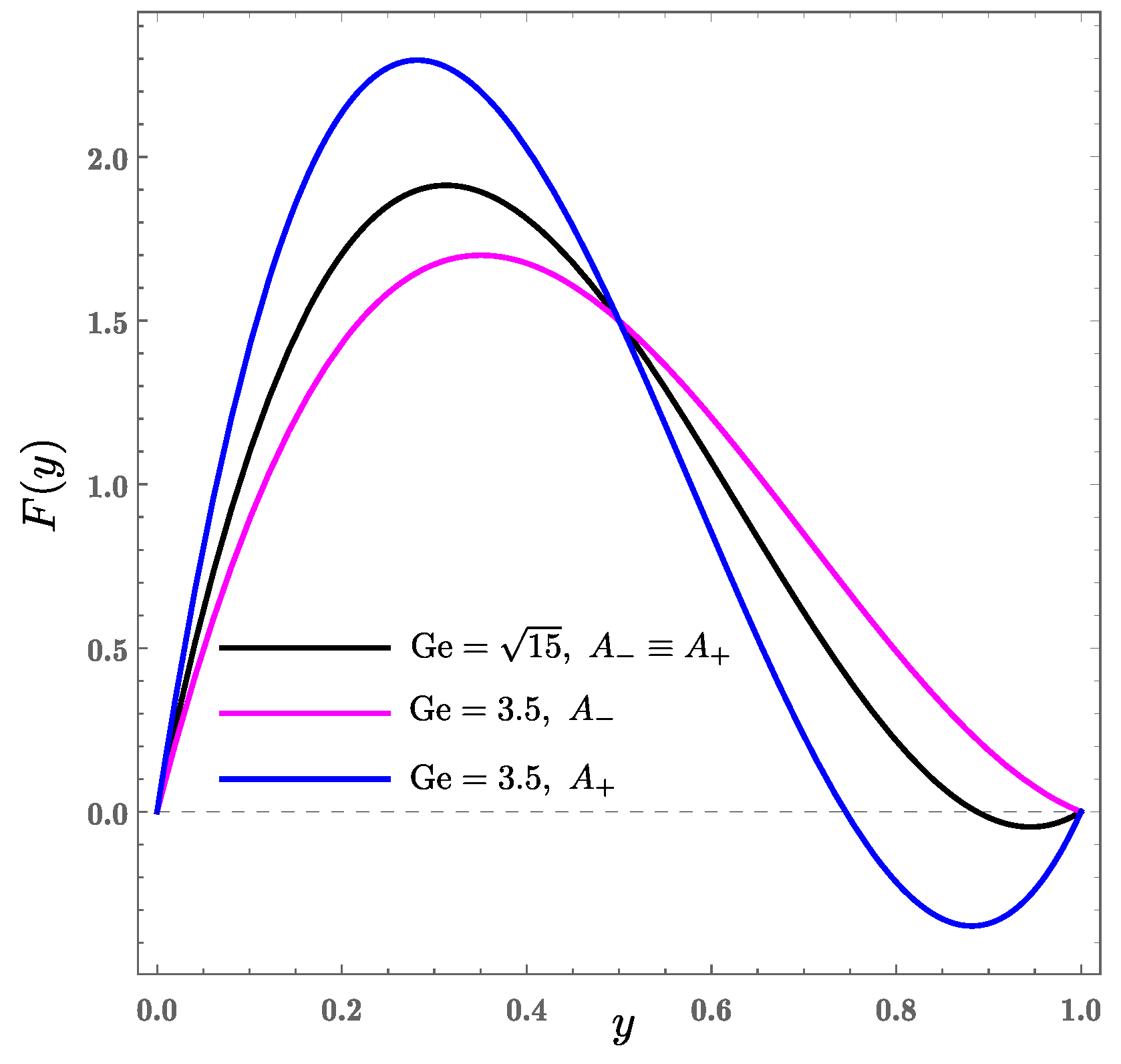
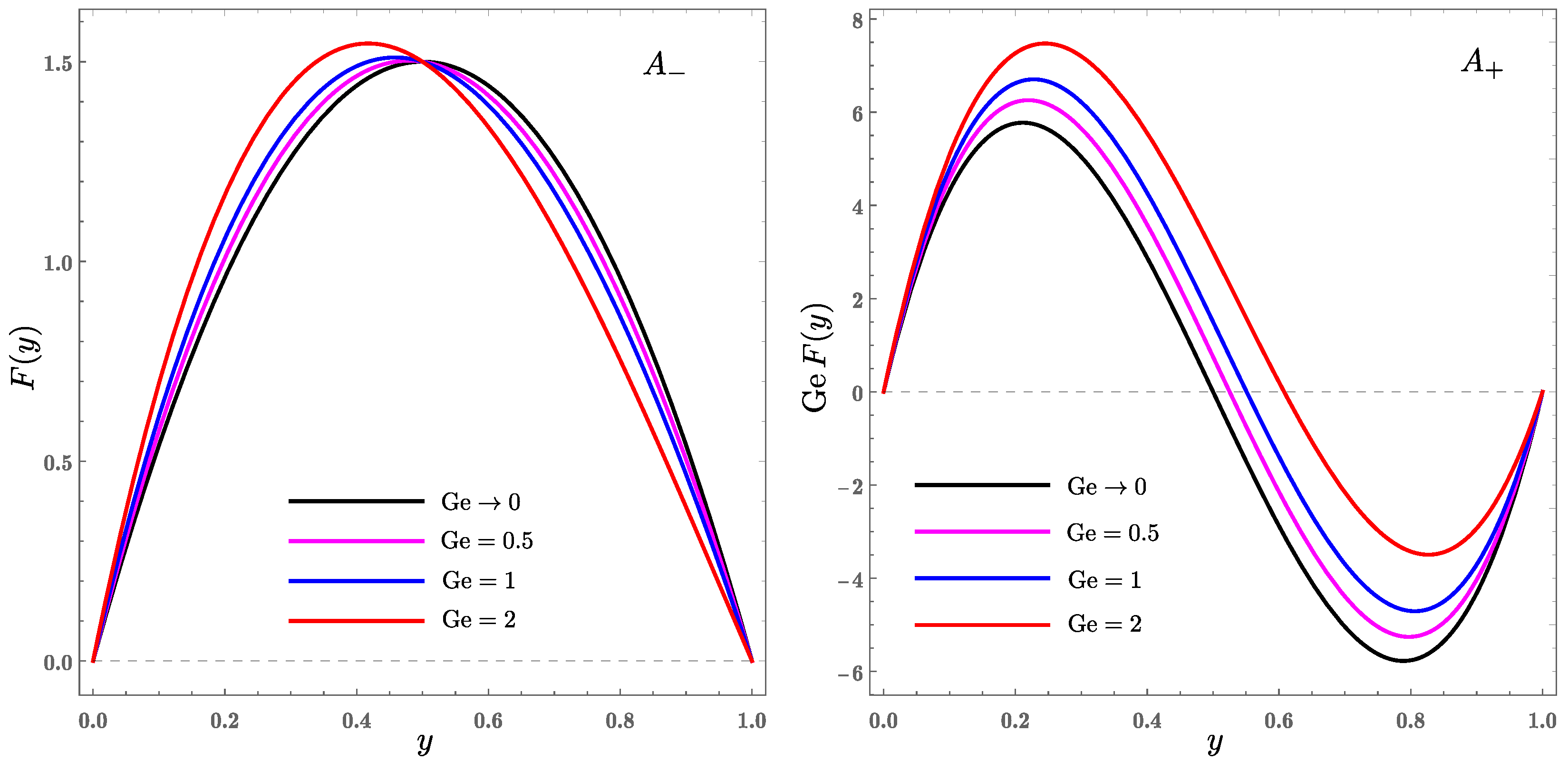
4.1. Characteristics of the Velocity Profiles

The deep diversity of features between the $A_{-}$–branch and $A_{+}$–branch emerges with the analysis of the velocity profiles. As $\mathrm{Pe}$ represents an overall scaling factor for the x–component of velocity, the velocity distribution in a $x=constant$ cross–section can be displayed by the function $F\left(y\right)$ and by its parametric dependence on the Gebhart number. This is made evident by Figure 2 where the dual branches $A_{-}$ and $A_{+}$ are illustrated for different values of Ge. A very wide range of Gebhart numbers is accounted for in Figure 2, from the limiting case $\mathrm{Ge}\to 0$ to $\mathrm{Ge}=2$. The latter value of Ge is really huge for most real-world applications except for geophysical applications where the channel width can be sufficiently large to achieve these Gebhart numbers. We bear in mind that Turcotte et al. [13] devised a range of Gebhart numbers up to $\mathrm{Ge}=3$.

Figure 2 features a left–hand frame with the $A_{-}$–branch velocity profiles and a right-hand frame with the $A_{+}$–branch velocity profiles. The comparison reveals that the two branches yield quite dissimilar profiles for a given Gebhart number. The $A_{-}$–branch shows slight departures from the Poiseuille velocity profile, which is exactly approached in the limit $\mathrm{Ge}\to 0$. This is rigorously proved by considering the lowest orders of a power series expansion of $F\left(y\right)$ with respect to Ge. In fact, from Equations (26) and (32) with $c_1=6+A_{-}$, one has

$$\begin{array}{c}F\left(y\right)\approx 6y(1-y)+y(1-y)(1-2y)\mathrm{Ge}+\dots ,\end{array}$$

(35)

where the zero–order term, and hence the limit of $F\left(y\right)$ for $\mathrm{Ge}\to 0$, is the Poiseuille profile. On account of Figure 2, the velocity profiles for the $A_{-}$–branch display a gradual, yet slight, loss of symmetry as Ge increases above zero. The cause of the asymmetry is the buoyancy effect produced by the viscous dissipation. Even when Ge moves close to its largest value compatible with the existence of the dual solutions, $\mathrm{Ge}=\sqrt{15}$, the departure from the Poiseuille profile becomes marked but not extremely large, as illustrated in Figure 3. The black line in Figure 3 displays the merging $A_{-}$ and $A_{+}$ profiles for $\mathrm{Ge}=\sqrt{15}$. We note that the merging velocity profiles display a bidirectional character with a flow reversal region close to $y=1$.

Flow reversal is a permanent property of the $A_{+}$–branch, as shown by both Figure 2 and Figure 3. On the other hand, the $A_{-}$–branch displays flow reversal close to the upper boundary only in the narrow range $15/4<\mathrm{Ge}\le \sqrt{15}$, as it can be easily inferred from Equations (26) and (32) with $c_1=6+A_{-}$. Figure 2 shows that the velocity profiles of the $A_{+}$–branch are bidirectional. The choice of plotting $\mathrm{Ge}F\left(y\right)$ in this case is a consequence of the singular behaviour of the $A_{+}$ profile $F\left(y\right)$ when $\mathrm{Ge}\to 0$. This feature is immediately gathered on evaluating, from Equations (26) and (32), the lowest orders of a power series expansion of $F\left(y\right)$ with respect to Ge with $c_1=6+A_{+}$,

$$\begin{array}{c}F\left(y\right)\approx \frac{60y(1-y)(1-2y)}{\mathrm{Ge}}+6y(1-y)-y(1-y)(1-2y)\mathrm{Ge}+\dots .\end{array}$$

(36)

By employing Equation (36), one obtains

$$\begin{array}{c}\underset{\mathrm{Ge}\to 0}{lim}\mathrm{Ge}F\left(y\right)=60y(1-y)(1-2y).\end{array}$$

(37)

The right–hand side of Equation (37) is a cubic polynomial profile describing an odd function of the shifted coordinate $y^{*}=y-1/2$.

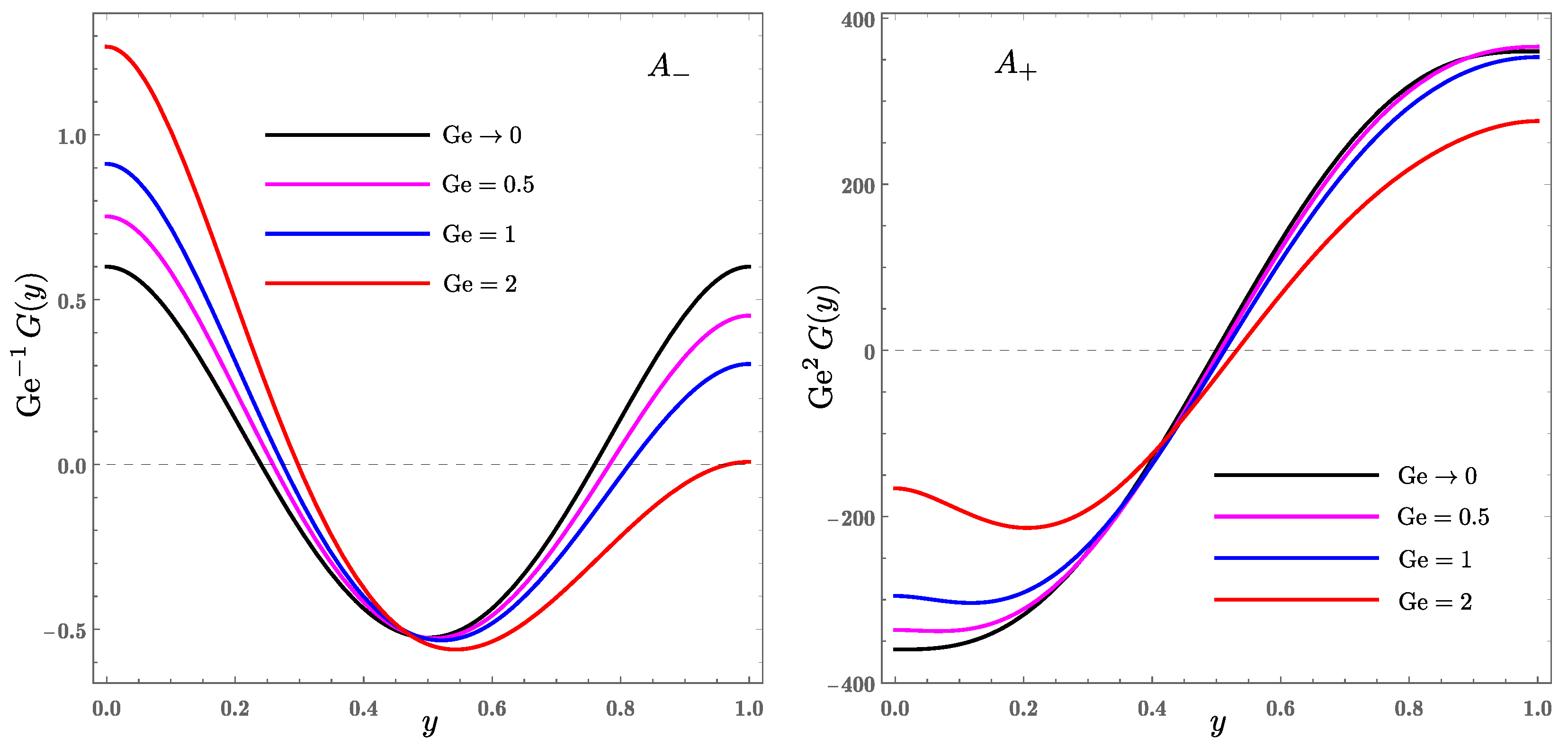
4.2. Characteristics of the Temperature Profiles

If function $F\left(y\right)$ represents the velocity distribution in a $x=constant$ cross–section, the temperature profile at $x=constant$ can be displayed by plotting function $G\left(y\right)$ as given by Equations (32) and (33).

Figure 4 shows that the $A_{-}$–branch yields an asymptotic temperature profile in the limit $\mathrm{Ge}\to 0$. This temperature profile is that corresponding to the forced convection regime where the Poiseuille profile describes velocity. In fact, this conclusion is supported by Equations (32) and (33) when we evaluate the lowest orders of a power series expansion of $G\left(y\right)$ with respect to Ge with $c_1=6+A_{-}$,

$$\begin{array}{c}G\left(y\right)\approx -3\left(6y^4-12y^3+6y^2-\frac{1}{5}\right)\mathrm{Ge}\\ +3\left(\frac{14}{5}{y}^5-7y^4+6y^3-2y^2+\frac{1}{10}\right){\mathrm{Ge}}^2+\dots .\end{array}$$

(38)

The black line in the left–hand frame of Figure 4 displays the fourth–order polynomial that appears in Equation (38) multiplied by Ge. Hence, the choice of plotting the scaled function ${\mathrm{Ge}}^{-1}G\left(y\right)$ for the $A_{-}$–branch profiles in Figure 4 is meant to capture the forced convection asymptotic case, where the buoyancy force is neglected with respect to the dynamic pressure gradient contribution in the local momentum balance. The $A_{-}$ temperature profiles displayed in Figure 4 for nonzero Ge display a departure from the symmetric temperature distribution in the forced convection limit, $\mathrm{Ge}\to 0$. As for the velocity profiles, the asymmetry is induced by the effects of the buoyancy force.

A power series expansion of $G\left(y\right)$, analogous to Equation (38), can be written for the $A_{+}$–branch,

$$\begin{array}{c}G\left(y\right)\approx \frac{360\left(12y^5-30y^4+20y^3-1\right)}{{\mathrm{Ge}}^2}\\ -\frac{12(2520y^6-7560y^5+8610y^4-4620y^3+1050y^2-17)}{7\mathrm{Ge}}\\ +(288y^5-720y^4+720y^3-360y^2+36)+\dots .\end{array}$$

(39)

The singular behaviour of the $A_{+}$–branch for $\mathrm{Ge}\to 0$ is highlighted by Equation (39). In the limit $\mathrm{Ge}\to 0$, the velocity diverges with ${\mathrm{Ge}}^{-1}$, as shown by Equation (36), while the temperature diverges with ${\mathrm{Ge}}^{-2}$. This limiting behaviour is the reason for the scaling, ${\mathrm{Ge}}^{2}G\left(y\right)$, used in the right–hand frame of Figure 4.

Figure 5 serves to complete the analysis of the dual temperature profiles in a regime of extremely large Gebhart numbers close to the upper threshold, $\mathrm{Ge}=\sqrt{15}$, above which no stationary parallel solutions are allowed. The merging of the two branches, $A_{-}$ and $A_{+}$, is illustrated by this figure.

Figure 4 and Figure 5, together with Equation (26), show that $\partial T/\partial y$ is negative in the lower part of the channel for the $A_{-}$–branch. Physically, this means a possibly unstable thermal stratification of the fluid that may give rise to a thermal instability of the flow. As already pointed out in Section 3.3, a stability analysis is beyond the scope of this paper, but the possible onset of the instability may be an interesting chance for future developments of this research. If the possibility of a thermally unstable behaviour of the $A_{-}$–branch is realistic, this phenomenon seems much less conceivable for the $A_{+}$–branch. In fact, for the $A_{+}$–branch, an unstable thermal stratification in the lower part of the channel is present, but it is counterbalanced, to a large extent, by a markedly stable thermal stratification in the largest part of the channel. If the $A_{+}$–branch is the physically unexpected feature of the solution obtained in Section 3, such an unexpected result is unlikely to be ruled out by a stability analysis. A similar conclusion is drawn in Barletta and Rees [10] with reference to the fluid flow in a saturated porous channel.

4.3. Are the Dual Flows Compatible with the Boussinesq Approximation?

The governing Equation (2) represents the widely employed Boussinesq approximation of the local mass, momentum and energy balance equations. As pointed out by several authors [14,15,16,17], the Boussinesq approximation is a correction to a fully–incompressible, constant properties flow model where the small effect taken into account is the buoyancy force. As such, the Boussinesq approximation corresponds to an asymptotic regime where a dimensionless parameter,

$$\begin{array}{c}ϵ=\beta \Delta T_{eff},\end{array}$$

(40)

tends to zero. Here, $\Delta T_{eff}$ is the actual maximum dimensional temperature difference occurring in the flow domain. We mention that the conceptualisation of buoyancy–induced flows where the approximate scheme is obtained in the asymptotic case $ϵ\to 0$ is already quite clearly laid out in the pioneering paper by Boussinesq [18].

The often overlooked situation is when the solution of the Boussinesq approximate equations is incompatible with the smallness of $\epsilon$. In rare cases, such a situation may arise even for perfectly reasonable values of the dimensionless parameter(s) governing the flow. In our case, the governing parameter is the Gebhart number which is assumed to be finite, though small enough. By considering the small–Ge expansion of the dimensionless temperature for the $A_{+}$–branch, Equation (39), we can approximate the maximum dimensionless temperature difference on a $x=constant$ cross–section as

$$\begin{array}{c}{T}_{max}-T_{min}\approx \frac{720{\mathrm{Pe}}^2}{{\mathrm{Ge}}^2},\end{array}$$

(41)

where Equation (26) has been also employed. Thus, Equations (6), (11), (40) and (41) lead to an expression of $ϵ$ for the $A_{+}$–branch at small Gebhart numbers,

$$\begin{array}{c}ϵ=\beta (T_{max}-T_{min})\frac{\alpha \nu }{g\beta H^3}\approx \frac{720Pr{\mathrm{Fr}}^2}{{\mathrm{Ge}}^2},\end{array}$$

(42)

where $\mathrm{Fr}$ is the Froude number based on the dimensional average velocity across the channel,

$$\begin{array}{c}\mathrm{Fr}=\frac{U_0}{\sqrt{gH}}.\end{array}$$

(43)

Equation (42) discloses the reason why the $A_{+}$–branch is incompatible with the asymptotic regime $ϵ\to 0$ characteristic of the Boussinesq approximation. In fact, the Gebhart number is usually small and the smaller is Ge the larger $ϵ$ is according to Equation (42). Therefore, the only chance to obtain a compatibility between the $A_{+}$–branch and the core assumption of the Boussinesq approximation, i.e., the limit $ϵ\to 0$, is considering large Gebhart numbers which, as suggested by Figure 4 and Figure 5, yield definitely smaller differences $T_{max}-T_{min}$. However, such large Gebhart numbers can be observed only with extremely wide flow systems such as those typical of geophysical or astrophysical applications.

5. Conclusions

The analysis of stationary two–dimensional mixed convection in a horizontal plane channel bounded by adiabatic walls was performed by taking into account the effect of the viscous dissipation caused by the forced flow rate across the channel. The velocity field was assumed to be parallel and directed along the horizontal x–axis. Under such conditions, the buoyancy force yields an effect exploited as a flow duality: two branches of possible flows exist denoted as the $A_{-}$–branch and $A_{+}$–branch.

Dual flows, $A_{-}$ and $A_{+}$, are allowed for every prescribed pair of input parameters $(\mathrm{Ge},\mathrm{Pe})$, where Ge is the Gebhart number and $\mathrm{Pe}$ is the Péclet number, provided that $\mathrm{Ge}\le \sqrt{15}$. The dual flows were obtained as completely analytical solutions of the local balance equations under the Boussinesq approximation. Such solutions have been expressed as polynomials with respect to the vertical y coordinate.

The dual flows exhibit quite diverse features, with the $A_{-}$–branch showing up small departures from the forced convection limit of Poiseuille flow at small Gebhart numbers, and the $A_{+}$–branch displaying bidirectional flows with a singular behaviour as Ge tends to zero.

The compatibility between the dual flows and the Boussinesq approximation was discussed. The proposed arguments led us to a scenario where the dual flows yield a conceivable behaviour, for the $A_{-}$–branch, which is characterised by small asymmetric departures from the Poiseuille velocity profile. The other branch, $A_{+}$, has characteristics to a large extent incompatible with the asymptotic nature of the Boussinesq approximation intended as the limiting case where $ϵ\to 0$, where $ϵ=\beta \Delta T_{eff}$ with $\beta$ the thermal expansion coefficient and $\Delta T_{eff}$ the maximum dimensional temperature difference within the flow domain.

A challenge for a future development of this analysis is the investigation of a scheme different from the Boussinesq approximation, which may lead to a self–consistent framework of flow duality, where the features of both branches can be determined in a reliable way. Among the many possibilities, one can employ the Gay–Lussac approximation outlined by Mayeli and Sheard [17] or a more complex fully compressible scheme along the lines drawn, for instance in the analysis carried out by Chenoweth and Paolucci [19].

References

- Batchelor, G.K. Heat transfer by free convection across a closed cavity between vertical boundaries at different temperatures. Q. Appl. Math. 1954, 12, 209–233. [Google Scholar] [CrossRef] [Green Version]
- Barletta, A.; Magyari, E.; Keller, B. Dual mixed convection flows in a vertical channel. Int. J. Heat Mass Transf. 2005, 48, 4835–4845. [Google Scholar] [CrossRef]
- Barletta, A.; Magyari, E.; Pop, I.; Storesletten, L. Mixed convection with viscous dissipation in a vertical channel filled with a porous medium. Acta Mech. 2007, 194, 123–140. [Google Scholar] [CrossRef]
- Barletta, A.; Lazzari, S.; Magyari, E. Buoyant Poiseuille-Couette flow with viscous dissipation in a vertical channel. Z. Angew. Math. Phys. 2008, 59, 1039–1056. [Google Scholar] [CrossRef]
- Miklavčič, M.; Wang, C.Y. Completely passive natural convection. Z. Angew. Math. Mech. 2011, 91, 601–606. [Google Scholar] [CrossRef] [Green Version]
- Miklavčič, M. Stability analysis of some fully developed mixed convection flows in a vertical channel. Z. Angew. Math. Mech. 2015, 95, 982–986. [Google Scholar] [CrossRef]
- Barletta, A.; Miklavčič, M. On fully developed mixed convection with viscous dissipation in a vertical channel and its stability. Z. Angew. Math. Mech. 2016, 96, 1457–1466. [Google Scholar] [CrossRef]
- Gebhart, B. Effects of viscous dissipation in natural convection. J. Fluid Mech. 1962, 14, 225–232. [Google Scholar] [CrossRef]
- Gebhart, B.; Mollendorf, J. Viscous dissipation in external natural convection flows. J. Fluid Mech. 1969, 38, 97–107. [Google Scholar] [CrossRef]
- Barletta, A.; Rees, D.A.S. Stability analysis of dual adiabatic flows in a horizontal porous layer. Int. J. Heat Mass Transf. 2009, 52, 2300–2310. [Google Scholar] [CrossRef]
- Barletta, A.; Zanchini, E. On the choice of the reference temperature for fully–developed mixed convection in a vertical channel. Int. J. Heat Mass Transf. 1999, 42, 3169–3181. [Google Scholar] [CrossRef]
- Normand, C.; Pomeau, Y.; Velarde, M.G. Convective instability: A physicist’s approach. Rev. Mod. Phys. 1977, 49, 581–624. [Google Scholar] [CrossRef]
- Turcotte, D.L.; Hsui, A.T.; Torrance, K.E.; Schubert, G. Influence of viscous dissipation on Bénard convection. J. Fluid Mech. 1974, 64, 369–374. [Google Scholar] [CrossRef]
- Zeytounian, R.K. The Bénard problem for deep convection: Rigorous derivation of approximate equations. Int. J. Eng. Sci. 1989, 27, 1361–1366. [Google Scholar] [CrossRef]
- Hills, R.N.; Roberts, P.H. On the motion of a fluid that is incompressible in a generalized sense and its relationship to the Boussinesq approximation. In Magnetohydrodynamics and the Earth’s Core: Selected Works by Paul Roberts; Soward, A.M., Ed.; CRC Press: London, UK, 2003; pp. 264–271. [Google Scholar]
- Rajagopal, K.R.; Ruzicka, M.; Srinivasa, A.R. On the Oberbeck–Boussinesq approximation. Math. Model. Methods Appl. Sci. 1996, 6, 1157–1167. [Google Scholar] [CrossRef]
- Mayeli, P.; Sheard, G.J. Buoyancy-driven flows beyond the Boussinesq approximation: A brief review. Int. Commun. Heat Mass Transf. 2021, 125, 105316. [Google Scholar] [CrossRef]
- Boussinesq, J. Mise en équation des phénomenes de convection calorifique et aperçu sur le pouvoir refroidissant des fluides. Journal de Physique Théorique et Appliquée 1902, 1, 65–71. [Google Scholar] [CrossRef]
- Chenoweth, D.R.; Paolucci, S. Gas flow in vertical slots with large horizontal temperature differences. Phys. Fluids 1985, 28, 2365–2374. [Google Scholar] [CrossRef]
Publisher’s Note: MDPI stays neutral with regard to jurisdictional claims in published maps and institutional affiliations. |
© 2022 by the authors. Licensee MDPI, Basel, Switzerland. This article is an open access article distributed under the terms and conditions of the Creative Commons Attribution (CC BY) license (https://creativecommons.org/licenses/by/4.0/).
Share and Cite
Barletta, A.; Celli, M.; Brandão, P.V. On Mixed Convection in a Horizontal Channel, Viscous Dissipation and Flow Duality. Fluids 2022, 7, 170. https://doi.org/10.3390/fluids7050170
Barletta A, Celli M, Brandão PV. On Mixed Convection in a Horizontal Channel, Viscous Dissipation and Flow Duality. Fluids. 2022; 7(5):170. https://doi.org/10.3390/fluids7050170
Chicago/Turabian StyleBarletta, Antonio, Michele Celli, and Pedro Vayssière Brandão. 2022. "On Mixed Convection in a Horizontal Channel, Viscous Dissipation and Flow Duality" Fluids 7, no. 5: 170. https://doi.org/10.3390/fluids7050170
APA StyleBarletta, A., Celli, M., & Brandão, P. V. (2022). On Mixed Convection in a Horizontal Channel, Viscous Dissipation and Flow Duality. Fluids, 7(5), 170. https://doi.org/10.3390/fluids7050170