
Tomographic Particle Image Velocimetry and Dynamic Mode Decomposition (DMD) in a Rectangular Impinging Jet: Vortex Dynamics and Acoustic Generation

 , ,
, ,
Abstract
:1. Introduction
2. Theoretical Background: DMD Method
3. Experimental Setup
3.1. Impinging Jet
3.2. Tomographic PIV
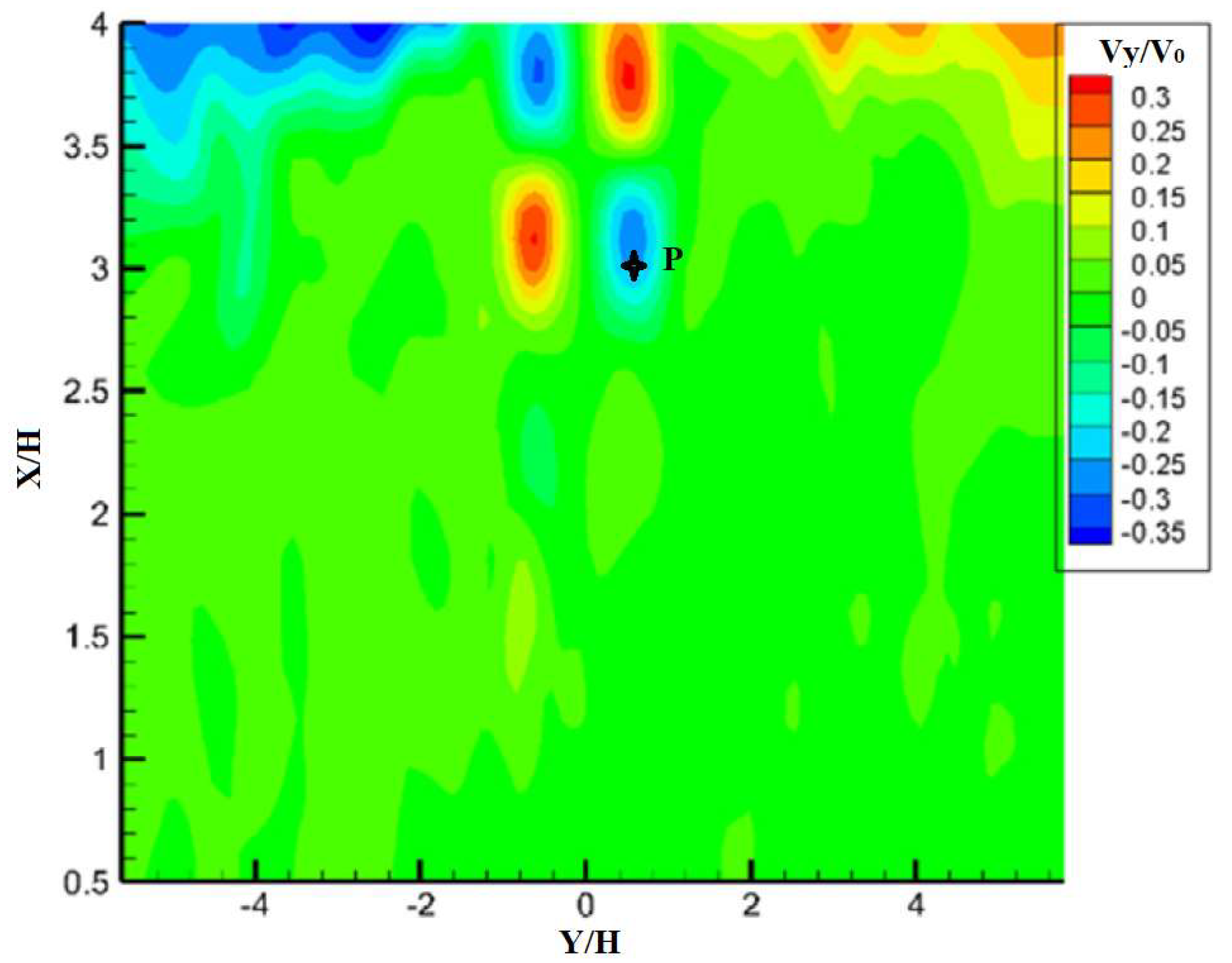
4. Results
4.1. Reconstruction of the Flow
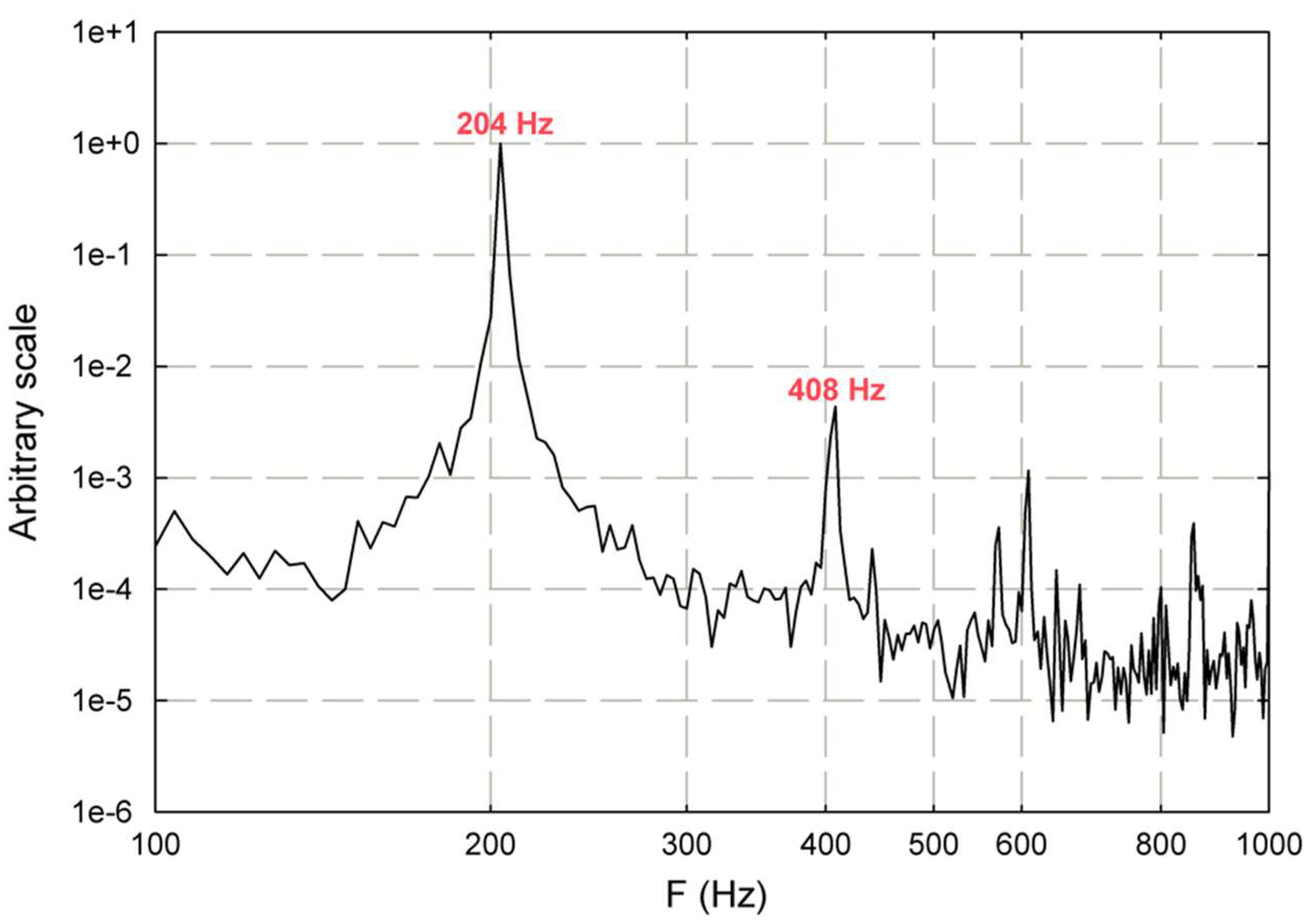
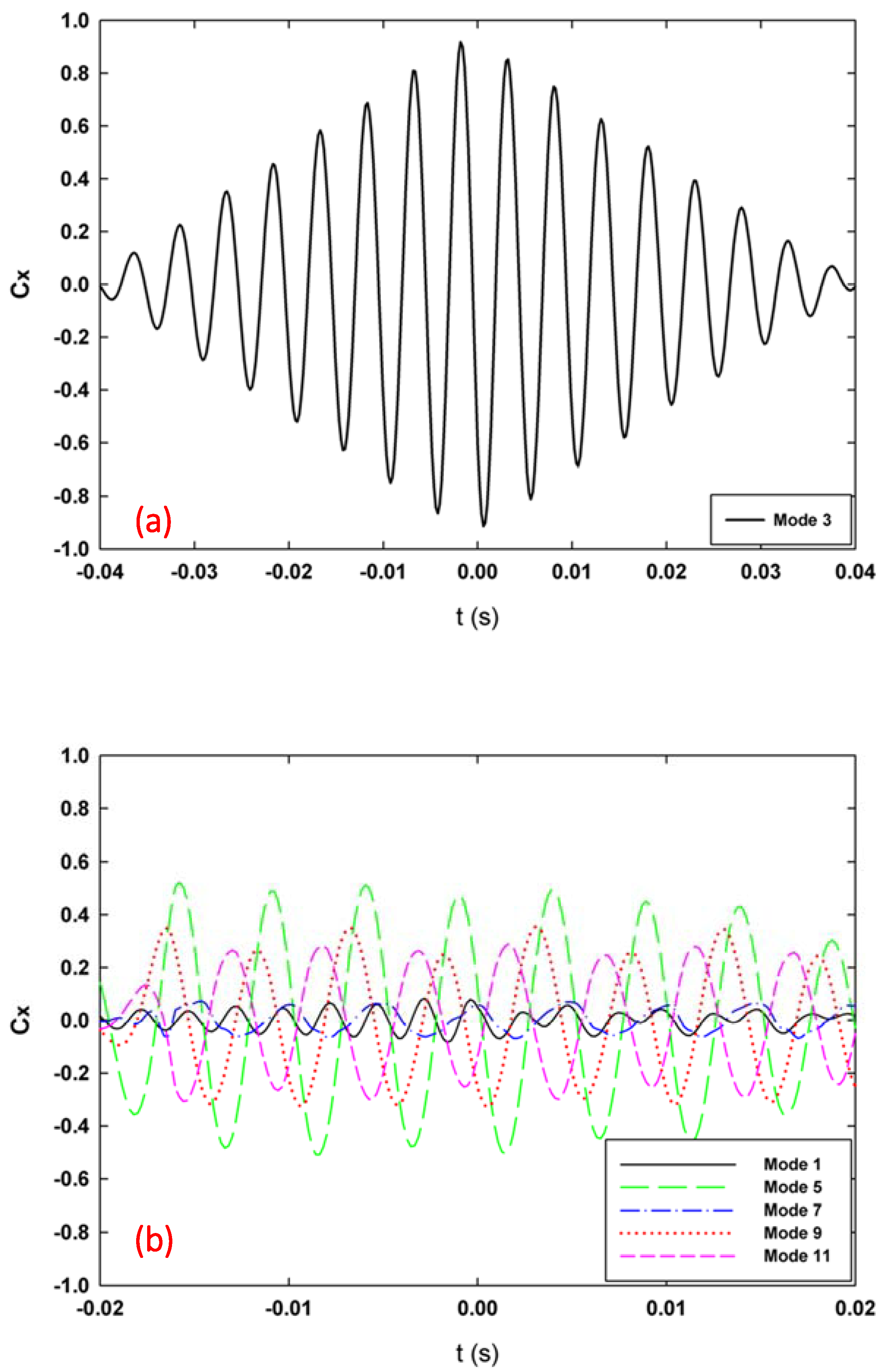
4.2. Spectral Content of the DMD Modes
5. Conclusions
Author Contributions
Funding
Acknowledgments
Conflicts of Interest
References
- Guckenheimer, J. Strange attractors in fluids: Another view. Annu. Rev. Fluid Mech. 1986, 18, 15–29. [Google Scholar] [CrossRef]
- Rowley, C.W.; Dawson, S.T. Model reduction for flow analysis and control. Annu. Rev. Fluid Mech. 2017, 49, 387–417. [Google Scholar] [CrossRef] [Green Version]
- Sirovich, L. Turbulence and dynamics of coherent structures Part I: Coherent structures. Q. Appl. Math. 1987, 45, 561–571. [Google Scholar] [CrossRef] [Green Version]
- Berkooz, G.; Holmes, P.; Lumley, J.L. The proper orthogonal decomposition in the analysis of turbulent flows. Annu. Rev. Fluid Mech. 1993, 25, 539–575. [Google Scholar] [CrossRef]
- Rowley, C.W.; Colonius, T.; Murray, R. Model reduction for compressible flows using POD and Galerkin projection. Phys. D Nonlinear Phenom. 2004, 189, 115–129. [Google Scholar] [CrossRef]
- Rowley, C. Model reduction for fluids, using balanced proper orthogonal decomposition. Int. J. Bifurc. Chaos 2005, 15, 997–1013. [Google Scholar] [CrossRef] [Green Version]
- Schmid, P.J. Dynamic mode decomposition of numerical and experimental data. J. Fluid Mech. 2010, 656, 5–28. [Google Scholar] [CrossRef] [Green Version]
- Tu, J.H.; Rowley, C.W.; Luchtenburg, D.M.; Brunton, S.L.; Kutz, J.N. On dynamic mode decomposition: Theory and applications. J. Comput. Dyn. 2014, 1, 391–421. [Google Scholar] [CrossRef] [Green Version]
- Mezić, I. Spectral properties of dynamical systems, model reduction and decompositions. Nonlinear Dyn. 2005, 41, 309–325. [Google Scholar] [CrossRef]
- Rowley, C.W.; Mezić, I.; Bagheri, S.; Schlatter, P.; Henningson, D.S. Spectral analysis of nonlinear flows. J. Fluid Mech. 2009, 641, 115–127. [Google Scholar] [CrossRef] [Green Version]
- Brunton, S.L.; Proctor, J.L.; Tu, J.H.; Kutz, J.N. Compressed sensing and dynamic mode decomposition. J. Comput. Dyn. 2015, 2, 165–191. [Google Scholar] [CrossRef]
- Kutz, J.N.; Fu, X.; Brunton, S.L. Multiresolution dynamic mode decomposition. SIAM J. Appl. Dyn. Syst. 2016, 15, 713–735. [Google Scholar] [CrossRef] [Green Version]
- Proctor, J.L.; Brunton, S.L.; Kutz, J.N. Dynamic mode decomposition with control. SIAM J. Appl. Dyn. Syst. 2016, 15, 142–161. [Google Scholar] [CrossRef] [Green Version]
- Seena, A.; Sung, H.J. Dynamic mode decomposition of turbulent cavity flows for self-sustained oscillations. Int. J. Heat Fluid Flow 2011, 32, 1098–1110. [Google Scholar] [CrossRef]
- Muld, T.W.; Efraimsson, G.; Henningson, D.S. Flow structures around a high-speed train extracted using proper orthogonal decomposition and dynamic mode decomposition. Comput. Fluids 2012, 57, 87–97. [Google Scholar] [CrossRef]
- Wang, T. Dynamic mode decomposition on LES result of cylinder cascade wake. In Proceedings of the 5th International Conference of Fluid Flow, Heat and Mass Transfer, Niagara Falls, ON, Canada, 7–9 June 2017. [Google Scholar]
- Liu, Y.; Zhang, Q. Dynamic mode decomposition of separated flow over a finite blunt plate: Time-resolved particle image velocimetry measurements. Exp. Fluids 2015, 56, 148. [Google Scholar] [CrossRef]
- Meslem, A.; Sobolik, V.; Bode, F.; Sodjavi, K.; Zaouali, Y.; Nastase, I.; Croitoru, C.V. Flow dynamics and mass transfer in impinging circular jet at low Reynolds number. Comparison of convergent and orifice nozzles. Int. J. Heat Mass Transf. 2013, 67, 25–45. [Google Scholar] [CrossRef]
- Semeraro, O.; Bellani, G.; Lundell, F. Analysis of time-resolved PIV measurements of a confined turbulent jet using POD and Koopman modes. Exp. Fluids 2012, 53, 1203–1220. [Google Scholar] [CrossRef]
- Ho, C.-M.; Nosseir, N.S. Dynamics of an impinging jet Part 1: The feedback phenomenon. J. Fluid Mech. 1981, 105, 119–142. [Google Scholar] [CrossRef]
- Ho, C.-M.; Nosseir, N.S. Large Coherent Structures in an Impinging Turbulent Jet. 1979. Available online: http://adsabs.harvard.edu/abs/1979stsf.procR.7H (accessed on 4 April 2017).
- Assoum, H.H.; El Hassan, M.; Abed-Meraim, K.; Sakout, A. The vortex dynamics and the self sustained tones in a plane jet impinging on a slotted plate. Eur. J. Mech. B Fluids 2014, 48, 231–235. [Google Scholar] [CrossRef]
- El Hassan, M.; Meslem, A. Time-resolved stereoscopic particle image velocimetry investigation of the entrainment in the near field of circular and daisy-shaped orifice jets. Phys. Fluids 2010, 22, 035107. [Google Scholar] [CrossRef]
- El Hassan, M.; Meslem, A.; Abed-Meraim, K. Experimental investigation of the flow in the near-field of a cross-shaped orifice jet. Phys. Fluids 2011, 23, 045101. [Google Scholar] [CrossRef]
- Assoum, H.H.; El Hassan, M.; Abed-Meraïm, K.; Martinuzzi, R.; Sakout, A. Experimental analysis of the aero-acoustic coupling in a plane impinging jet on a slotted plate. Fluid Dyn. Res. 2013, 45, 045503. [Google Scholar] [CrossRef]
- Hamdi, J.; Assoum, H.H.; Abed-Meraïm, K.; Sakout, A. Analysis of the effect of the 3C kinematic field of a confined impinging jet on a slotted plate by stereoscopic PIV. Eur. J. Mech. B Fluids 2019, 76, 243–258. [Google Scholar] [CrossRef]
- Hamdi, J.; Assoum, H.; Abed-Meraïm, K.; Sakout, A. Volume reconstruction of an impinging jet obtained from stereoscopic-PIV data using POD. Eur. J. Mech. B Fluids 2018, 67, 433–445. [Google Scholar] [CrossRef]
- Assoum, H.H.; Hamdi, J.; Abed-Meraïm, K.; Al Kheir, M.; Mrach, T.; El Soufi, L.; Sakout, A. Spatio-temporal changes in the turbulent kinetic energy of a rectangular jet impinging on a slotted plate analyzed with High Speed 3D tomographic-particle image velocimetry. Int. J. Heat Technol. 2019, 37, 1071–1079. [Google Scholar] [CrossRef] [Green Version]
- Assoum, H.; Hamdi, J.; Abed-Meraim, K.; El Hassan, M.; Ali, M.; Sakout, A. Correlation between the acoustic field and the transverse velocity in a plane impinging jet in the presence of self-sustaining tones. Energy Procedia 2017, 139, 391–397. [Google Scholar] [CrossRef]
- Assoum, H.H.; Hamdi, J.; El Hassan, M.; Kamel, A.M.; Kheir, M.E.; Mrach, T.; Asmar, S.E.; Anas, S. Turbulent kinetic energy and self-sustaining tones in an impinging jet using High Speed 3D Tomographic-PIV. Energy Rep. 2020, 6, 6322–6333. [Google Scholar]
- El Hassan, M.; Assoum, H.H.; Martinuzzi, R.; Sobolik, V.; Abed-Meraim, K.; Sakout, A. Experimental investigation of the wall shear stress in a circular impinging jet. Phys. Fluids 2013, 25, 077101. [Google Scholar] [CrossRef]
- El Hassan, M.; Assoum, H.H.; Sobolik, V.; Vétel, J.; Abed-Meraim, K.; Garon, A.; Sakout, A. Experimental investigation of the wall shear stress and the vortex dynamics in a circular impinging jet. Exp. Fluids 2012, 52, 1475–1489. [Google Scholar] [CrossRef]
- Lusseyran, F.; Guéniat, F.; Basley, J.; Douay, C.L.; Pastur, L.R.; Faure, T.M.; Schmid, P.J. Flow coherent structures and frequency signature: Application of the dynamic modes decomposition to open cavity flow. J. Phys. Conf. Ser. 2011, 318, 042036. [Google Scholar] [CrossRef] [Green Version]
- Schmid, P.J. Application of the dynamic mode decomposition to experimental data. Exp. Fluids 2011, 50, 1123–1130. [Google Scholar] [CrossRef]
- Schmid, P.J.; Meyer, K.E.; Pust, O. Dynamic mode decomposition and proper orthogonal decomposition of flow in a lid-driven cylindrical cavity. In Proceedings of the 8th International Symposium on Particle Image Velocimetry, Melbourne, Australia, 25–28 August 2009. [Google Scholar]
- Schmid, P.J.; Li, L.; Juniper, M.; Pust, O. Applications of the dynamic mode decomposition. Theor. Comput. Fluid Dyn. 2010, 25, 249–259. [Google Scholar] [CrossRef]
- Kutz, J.N.; Brunton, S.L.; Brunton, B.W.; Proctor, J.L. Dynamic Mode Decomposition: Data-Driven Modeling of Complex Systems; Society for Industrial and Applied Mathematics: Philadelphia, PA, USA, 2016. [Google Scholar]
- Elsinga, G.E.; Scarano, F.; Wieneke, B.; van Oudheusden, B.W. Tomographic particle image velocimetry. Exp. Fluids 2006, 41, 933–947. [Google Scholar] [CrossRef]
- Sirovich, L.; Kirby, M. Low-dimensional procedure for the characterization of human faces. J. Opt. Soc. Am. A 1987, 4, 519–524. [Google Scholar] [CrossRef] [PubMed]
- Gavish, M.; Donoho, D.L. The optimal hard threshold for singular values is . IEEE Trans. Inf. Theory 2014, 60, 5040–5053. [Google Scholar] [CrossRef]


| Data matrices | |
| SVD | |
| DMD modes Փ | |
| System’s solution |
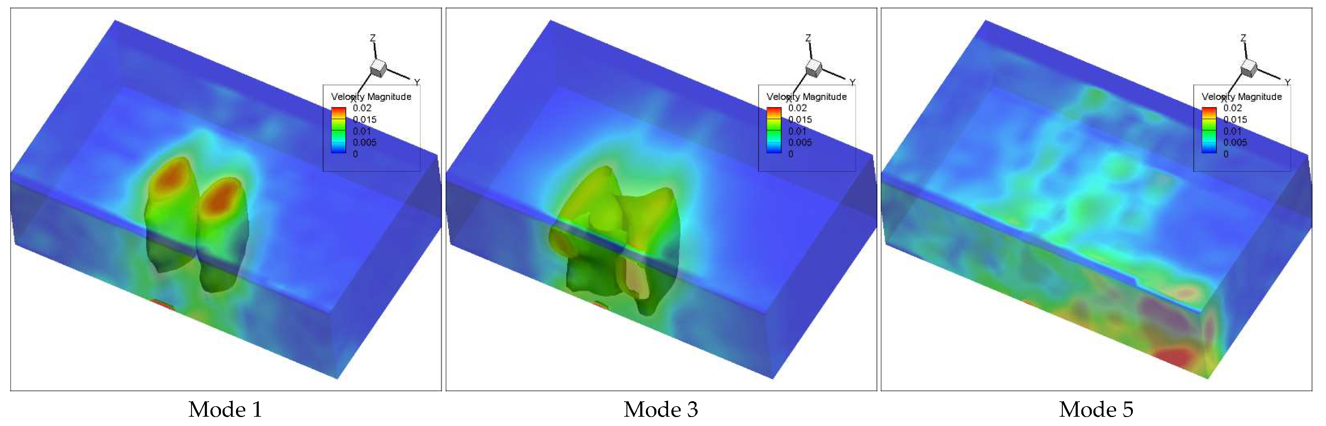
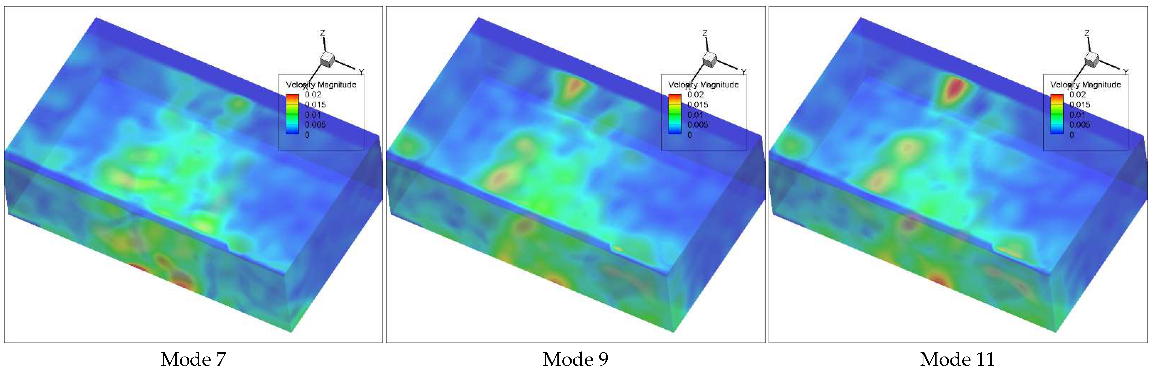
| DMD Mode | Frequency (Hz) |
|---|---|
| Mode 1 | 402.9 |
| Mode 3 | 200.7 |
| Mode 5 | 200.1 |
| Mode 7 | 610.1 |
| Mode 9 | 219.0 |
| Mode 11 | 220.2 |
Publisher’s Note: MDPI stays neutral with regard to jurisdictional claims in published maps and institutional affiliations. |
© 2021 by the authors. Licensee MDPI, Basel, Switzerland. This article is an open access article distributed under the terms and conditions of the Creative Commons Attribution (CC BY) license (https://creativecommons.org/licenses/by/4.0/).
Share and Cite
Assoum, H.H.; Hamdi, J.; Alkheir, M.; Abed Meraim, K.; Sakout, A.; Obeid, B.; El Hassan, M. Tomographic Particle Image Velocimetry and Dynamic Mode Decomposition (DMD) in a Rectangular Impinging Jet: Vortex Dynamics and Acoustic Generation. Fluids 2021, 6, 429. https://doi.org/10.3390/fluids6120429
Assoum HH, Hamdi J, Alkheir M, Abed Meraim K, Sakout A, Obeid B, El Hassan M. Tomographic Particle Image Velocimetry and Dynamic Mode Decomposition (DMD) in a Rectangular Impinging Jet: Vortex Dynamics and Acoustic Generation. Fluids. 2021; 6(12):429. https://doi.org/10.3390/fluids6120429
Chicago/Turabian StyleAssoum, Hassan H., Jana Hamdi, Marwan Alkheir, Kamel Abed Meraim, Anas Sakout, Bachar Obeid, and Mouhammad El Hassan. 2021. "Tomographic Particle Image Velocimetry and Dynamic Mode Decomposition (DMD) in a Rectangular Impinging Jet: Vortex Dynamics and Acoustic Generation" Fluids 6, no. 12: 429. https://doi.org/10.3390/fluids6120429
APA StyleAssoum, H. H., Hamdi, J., Alkheir, M., Abed Meraim, K., Sakout, A., Obeid, B., & El Hassan, M. (2021). Tomographic Particle Image Velocimetry and Dynamic Mode Decomposition (DMD) in a Rectangular Impinging Jet: Vortex Dynamics and Acoustic Generation. Fluids, 6(12), 429. https://doi.org/10.3390/fluids6120429