Uncertainty Quantification Methodologies Applied to the Rotor Tip Clearance Effect in a Twin Scroll Radial Turbine

Abstract

In the last three decades computer simulation tools have achieved wide spread use in the design and analysis of engineering devices. This has shortened the overall product design cycle (physical experiments may be impossible during early design stages) and it has also provided better understanding of the operating behavior of the systems under investigation. As a consequence numerical simulation have led to a reduction of physical prototyping and to lower costs for manufacturing production chains. Despite this success, it remains difficult to provide objective confidence levels in quantitative information derived from numerical predictions. The complexity arises from the amount of uncertainties related to the inputs of any computation attempting to represent a physical system. This paper focuses on geometrical sources of uncertainty in the field of CFD applied to twin scroll radial turbines. In particular it has been investigated the effect of uncertainties on tip clearance values at rotor blade leading edge and trailing edge on selected turbine performance parameters. The analysis shows the use of the Surrogate-based uncertainty quantification technique that has been setup by the authors in the Dakota^® environment. The polynomial chaos expansion method has been applied to the same case. The comparison of the results coming from the different approaches and the discussion of the pros and cons related to each technique lead to interesting conclusions, which are proposed as guidelines for future UQ applications on the theme of CFD applied to radial turbines.

1. Introduction

Uncertainty quantification is the science of characterizing and reducing uncertainties in both computational and real world applications, a tool for determining how likely certain outcomes are if aspects of the system are not completely known; while the models and methodologies (which combine mathematics, statistics and engineering) are used throughout academia, the practice has not been incorporated into professional engineering workflows. The uncertainty propagation through the CFD model supports engineers to determine whether system outputs will meet the requirements, what the extreme probabilities really are and which inputs have the most significant effect on output distributions.

A fundamental aspect to be considered in every simulation is represented by the differences between the real geometrical model (the actual manufactured machine) and the simulated one (the CFD model). The computational domain used in CFD to simulate a turbine and the real control volume are not identical; this is due to different factors [1]:

• the actual machine is different from the designer’s projects due to manufacturing (epistemic) and assembling (aleatory) uncertainties;
• usually the computational domain does not account for all geometrical features, such as fillets.

Moreover, it is noteworthy to mention that many authors [2,3] have already investigated the variability of gaps, fillets and small geometrical details due to the turbomachinery operating conditions. One of the most delicate geometrical aspects concerning radial turbines is undoubtedly the tip clearance, i.e., the gap between rotor tip and the shroud surface. Usually, in order to limit tip leakage flows, thus optimizing turbine performance, clearances are kept very close; in this scenario small geometrical variations, e.g., induced by harsh operating conditions, can be responsible of appreciable performance variations.

Epistemic uncertainties of a numerical model represent the level of uncertainty in reproducing a physical system or phenomenon, while the aleatory uncertainties are a strict property of the system being analyzed. Following this definition turbulence modeling is an epistemic uncertainty whose effect has been widely investigated at the rotor tip by Krishnababu et al. [4].

This paper deals with the operational aleatory uncertainties to which the tip clearances (at leading and trailing edge) of a twin entry turbine impeller are subjected: centrifugal, thermal, assembly and wear effects can significantly affect tip clearance values. The turbine under investigation is for automotive turbocharging and the authors have previously developed a numerical model for the simulation of this turbine, validated with experimental data [5]. The uncertainties propagation through the CFD model of the turbine has been performed using an automated procedure developed within the Dakota^® environment, an open source toolset provided with a large number of optimization and uncertainty quantification utilities.

Response surface methods have been widely employed for design optimization approaches [6,7], but the same techniques can also be very useful in the field of UQ methods based on sampling, in order to bypass the high computational cost generally required to generate converging statistics.

The first application of UQ methodologies follows a ‘Surrogate-based’ approach [8] already tested by the authors on a case study [9]. This method consists, at first, in the evaluation of the objective functions on a fixed set of samples (DoE), then the results are used to generate a surrogate model (RSM) of the underlying “true” functions. In the final step random sampling (using thousands of samples) is performed on the meta-model to obtain estimates of the mean, variance, and percentiles of the response functions.

The second UQ approach investigated is the Polynomial Chaos Expansion (PCE), which is based on a multidimensional orthogonal polynomial approximation formed in terms of standardized random variables. A distinguishing feature of this methodology is that the final solution is expressed as a functional mapping, and not merely as a set of statistics as in the case of many nondeterministic approaches. However, polynomial approaches suffer the curse of dimensionality [1], so their application is limited to cases where the number of uncertain variables is below 5 (as in this work), since the number of CFD simulations needed increases exponentially with the number of input variables considered.

At first, based on experience gained on radial turbines [5,10], some key performance parameters have been selected as response functions for the UQ analysis. According to experimental/CFD data available on radial turbines for turbocharging applications, the input probability distribution functions assigned to the rotor tip clearance were selected considering physically suitable values for both the average values and the standard deviations. The propagation through the CFD model of the input uncertainties on rotor tip clearances lead to the probability density functions (PDF) of the outputs; hence the statistical distributions from the two UQ methods (Surrogate-based and PCE) have been compared.

The final target is to highlight the pros and cons of each UQ technique applied to the numerical simulation of turbocharging radial turbines, leading to guidelines for future incorporation of uncertainty quantification procedures into industrial design workflows.

2. Turbine CFD Model

The test case turbine is a twin scroll inflow radial turbine for turbocharging applications. Geometrical and performance data are confidential then all quantities have been reported in the following in non-dimensional or reduced form. For volute and rotor geometrical details, the reader can refer to previous research works [5,10] which focus on a detailed study of the twin entry turbines fluid-dynamic behavior.

The ANSYS^® CFX commercial platform has been coupled to the Dakota open source for its UQ capabilities.

The twin scroll volute has been discretized with an unstructured mesh (prism layers added for guarantee for boundary layer resolution), as depicted in Figure 1, while a structured grid has been generated for the rotor. The blade leading (L.E.) and trailing (T.E.) edge are indicated in Figure 2.

The CFD model is divided into three domains (Figure 3): volute, single rotor channel, out.

The set of boundary conditions used for the different domains is reported in

Table 1. CFD model boundary conditions. Numbers define ‘in-out’ control sections for each domain.

Domain	Boundary Conditions
Volute (1–2)	- inlet total pressure and total temperature - flow direction normal to volute inlets
Rotor Channel (2–3)	- rotational speed - rotational periodicity on side walls - counter-rotating shroud wall
Out (3–4)	- static pressure on outlet section

.

Simulations were performed with steady-state flow condition and in full admission (for more details on twin entry admission conditions see [11,12]). The choice to simulate a fixed operating point is due to the necessity to isolate the effects of tip clearance uncertainties on selected turbine performance parameters. From the experimental maps provided by the customer, a working point at maximum rotational speed and near choke has been selected. This choice is because the highly stressed condition due to the following aspects is obtained:

• high internal combustion engine exhaust gas temperature → thermal stress;
• high peripheral speed values → centrifugal stress;
• high flow momentum variation and flow leakage in the backside cavity [5] → maximum thrust on bearings.

These factors can significantly reduce the ‘nominal’ tip clearance values, which have been assumed as the mean values of the corresponding probability density functions.

3. Input Uncertainties

The input uncertain variables of the uncertainty quantification problem are two: the tip clearance values at rotor leading edge and at the trailing edge, whose range of variations and statistic moments are summarized in

Table 2. Input uncertain variables range and statistics.

TIP CLEARANCE	LE [%h_bin]	TE [%h_bout]
min	1.00%	1.00%
MAX	9.00%	6.00%
ave	5.00%	3.50%
std deviation	0.50%	0.35%

. Normal distributions have been assumed for the two variables, as in Figure 4.

The clearance values are reported in Table 1 as a percentage of the corresponding blade heights. The standard deviation ($\sigma$—for the definition see Equation (2)) of the two input distributions has been assumed equal to 10% of the respective mean value.

According the Gaussian probability density function definition (Equation (1)) the 99.73% of input samples will be concentrated inside the ± 3$\sigma$ range centered on the mean value. Therefore the ‘min’ and ‘MAX’ clearance values reported in Table 2 identify the range of variation since the input samples of the UQ analysis will be almost totally included in the following ranges: TC_LE = 3.5–6.5%h_bin, TC_TE = 2.45–4.55%h_bout.

The maximum values of clearance inside the abovementioned ranges can realistically correspond to the cold blade, i.e., to the turbine start-up phase (i.e., when the internal combustion engine is fired up). The minimum values (‘min’) simulate the maximum stress conditions instead.

$$f_x\left(x\right)=\frac{1}{\sqrt{2\pi }\sigma }exp\left[\frac{-1}{2}{\left(\frac{x-\mu }{\sigma }\right)}^2\right]$$

(1)

$$\sigma =\sqrt{{\displaystyle \sum }_{i=1}^N\frac{1}{N-1}{\left(x_i-\mu \right)}^2}$$

(2)

The clearance variations are a consequence of the turbine blade deformation during service. Two main factors can explain this deformation:

• thermal stress, stronger at the LE where the hot gases have not yet undergone the expansion which produces a remarkable pressure and temperature drop;
• centrifugal stress (quadratic with rotational speed), stronger at the TE where the blade extends mainly in the radial direction, along which the centrifugal force acts.

The variation range (max-min) assigned at the LE is greater (in percentage terms) and this is related to a third contribution factor, i.e., the axial thrust on rotor bearings. On this issue many authors investigated [13,14] and discussed that the thrust contribution from the leakage flow in the rotor backside cavity is usually greater than the momentum variation contribution due to blade flow deflection. The overall thrust tends to push the rotor toward the shroud at the LE resulting in a further reduction of the existing gap (while at the TE the axial thrust has no effect on the clearance).

4. Response Functions

The response functions selected for this UQ problem are twin scroll radial turbine performance parameters, reported below for sake of completeness:

• overall expansion ratio, i.e., the ratio between volute inlet total pressure and tailpipe outlet static pressure. In the present turbine volute inlets cross sections are the same, thus it is valid to consider an arithmetic mean of inlets total pressures;

  $$PRF=\frac{p_{t1sh}+p_{t1hub}}{2p_4}$$

  (3)
• rotor expansion ratio ($PR{F}_{rotor}$), which has the same definition reported in Equation (3) but with the static pressure measured at rotor outlet (p3) instead of the outlet pressure (p4);
• mass flow ratio, i.e., the ratio between mass flow through one of the two branches and overall mass flow processed by the turbine;

  $$MF{R}_{sh}=\frac{{\dot{m}}_{sh}}{{\dot{m}}_{tot}};MF{R}_{hub}=\frac{{\dot{m}}_{hub}}{{\dot{m}}_{tot}}$$

  (4)
• mass flow parameter, used to estimate turbine flow swallowing capacity. In case of twin entries, MFP is calculated considering the contribution of each volute branch (‘hub’ or ‘shroud’ rotor side) on the overall mass flow;

  $$MFP={\dot{m}}_{tot}\frac{\sqrt{MF{R}_{sh}{T}_{t1sh}+MF{R}_{hub}{T}_{t1hub}}}{\frac{p_{t1sh}+p_{t1hub}}{2}}$$

  (5)
• Overall total to static efficiency, i.e., the ratio between the actual total enthalpy drop ($h_{01}-h_{04}$) and the total to static enthalpy variation in case of isentropic transformation from volute inlets to tailpipe outlet;

  $${\eta }_{ts}=\frac{1-\left(\frac{T_{t1}}{T_{t3}}\right)}{1-{\left(\frac{1}{PRF}\right)}^{\left(\frac{k-1}{k}\right)}}$$

  (6)
• Rotor total to static efficiency, which has the same definition reported in Equation (6) but with the rotor expansion ratio $PR{F}_{rotor}$ instead of the overall expansion ratio $PRF$.

A set of four response functions has been identified: $PR{F}_{rotor}$, $MFP$, ${\eta }_{t2s rotor}$, ${\eta }_{t2s}$.

5. UQ Techniques

The uncertainty quantification workflow involves the following steps:

• the UQ procedure gives the clearance values at rotor leading and trailing edge selected in the variation range according the input probability density functions specified in Dakota input file;
• the rotor mesh is then generated and imported in the computational model (ANSYS CFX^® platform);
• the CFD simulation is performed and the response functions values are extracted from post-processing and passed to the UQ algorithm.

This paper deals with the comparison of the results obtained with two different uncertainty quantification approaches: Surrogate-based sampling UQ and PCE.

5.1. Surrogate-Based Sampling UQ

At first a 64-samples Design of Experiments (DoE) has been generated with the Latin Hypercube Sampling [15] method: a reasonable number of numerical simulations is necessary to obtain, in the following phase, a meta-model which is a good approximation of the true physical model (the turbine CFD model). The input probability distributions are given to the sampling based UQ method (again LHS) which is applied to the response surface. The meta-model has been generated from the DoE through the Gaussian Process that involves techniques elaborated in the geostatistics and spatial statistics communities [16,17] to produce smooth surface fit models of the response values starting from a data set. The form of the GP model [8] is:

$$\hat{f}\left(\overline{x}\right)\approx \overline{g}{\left(\overline{x}\right)}^T\overline{\beta }+\overline{r}{\left(\overline{x}\right)}^T{\stackrel{=}{R}}^{-1} \left(\overline{f}-\stackrel{=}{G}\overline{\beta }\right)$$

(7)

where:

-

$\overline{x}$ is the current point in n-dimensional parameter space;

-

$\overline{g}\left(\overline{x}\right)$ is the vector of trend basis functions evaluated at $\overline{x}$;

-

$\overline{\beta }$ is a vector containing the generalized least squares estimates of the trend basis function coefficients;

-

$\overline{r}\left(\overline{x}\right)$ is the correlation vector of terms between $\overline{x}$ and the data points;

-

$\stackrel{=}{R}$ is the correlation matrix for all of the data points;

-

$\overline{f}$ is the vector of response values;

-

$\stackrel{=}{G}$ is the matrix containing the trend basis functions evaluated at all data points.

A Gaussian correlation function is used to compute the terms in the correlation vector and matrix which are dependent on an n-dimensional vector of correlation parameters $\overline{\theta }={\left\{{\theta }_1,\dots {\theta }_n\right\}}^T$ determined using a Maximum Likelihood Estimation (MLE) procedure.

The GP can be used to model surfaces with slope discontinuities along with multiple local minima and maxima because it has a hyper-parametric error model; this makes the Gaussian Process a very flexible tool for modeling response functions obtained from the simulation of complex fluid dynamic problems. The samples number of the sampling-based UQ is two order of magnitude greater than the corresponding number used for DoE generation; the input uncertainties propagate through the meta-model leading to the response function PDFs.

5.2. Polynomial Chaos Expansion

Polynomial chaos expansions (PCE) use multidimensional orthogonal polynomial approximation formed in terms of standardized random variables. Stochastic Expansion methods use the notions of projection, orthogonality, and weak convergence [18,19] in order to estimate the functional relationship between response functions and their random inputs, giving a more complete uncertainty representation for application in multi-code simulations.

The set of classical orthogonal polynomials that provide an optimal basis for different continuous probability distribution types is obtained from the family of hypergeometric orthogonal polynomials known as the Askey scheme [20]. If all random inputs can be described using independent normal, uniform, exponential, beta, and gamma distributions (as in the present work) then Askey polynomials can be directly applied. The set of polynomials are used as an orthogonal basis to approximate the functional form between the stochastic response output and each of its random inputs. The chaos expansion for a response R takes the form [21]:

$$R=a_0{B}_0+{\displaystyle \sum }_{i_1=1}^{\infty }{a}_{i_1}{B}_1\left({\xi }_{i_1}\right)+{\displaystyle \sum }_{i_1=1}^{\infty } {\displaystyle \sum }_{i_2=1}^{i_1}{a}_{i_1{i}_2}{B}_2\left({\xi }_{i_1},{\xi }_{i_2}\right)+{\displaystyle \sum }_{i_1=1}^{\infty }{\displaystyle \sum }_{i_2=1}^{i_1}{\displaystyle \sum }_{i_3=1}^{i_2}{a}_{i_1{i}_2{i}_3}{B}_3\left({\xi }_{i_1},{\xi }_{i_2},{\xi }_{i_3}\right)+\cdots$$

(8)

where the random vector dimension is unbounded and each additional set of nested summations corresponds to an additional order of polynomials in the expansion formulation. Using a more compact term-based indexing, the chaos expansion for a response R takes the general form:

$$R={\displaystyle \sum }_{j=0}^{\infty }{\alpha }_j{\psi }_j\left(\xi \right)$$

(9)

where there is a one-to-one correspondence between $a_{i_1 i_2 \dots i_n}$ and ${\alpha }_j$ and between $B_n\left({\xi }_{i_1},{\xi }_{i_2}\dots {\xi }_{i_n}\right)$ and ψ_j(ξ), which are multidimensional polynomials involving products of the one-dimensional polynomials. The further step consists in truncating the infinite expansion at a finite number of random variables (the input uncertain variables) and at a finite expansion order:

$$R\cong {\displaystyle \sum }_{j=0}^P{\alpha }_j{\psi }_j\left(\xi \right)$$

(10)

According to the “tensor-product expansion” approach [21] polynomial order bounds are used on a per-dimension basis and all combinations of the one-dimensional polynomials are counted; furthermore the tensor-product expansion contemplates anisotropy in polynomial order for each dimension (variable) since the polynomial order bounds for each dimension can be defined independently. PCE estimates the coefficients ${\alpha }_j$ using the spectral projection approach, which projects the response on every basis function using inner products and exploits the polynomial orthogonality properties to obtain each expansion coefficient:

$${\alpha }_j=\frac{\langle R,{\psi }_j\rangle }{\langle {\psi }_j{}^2\rangle }=\frac{1}{\langle {\psi }_j{}^2\rangle } {{\displaystyle \int }}_{\mathsf{\Omega }}R {\psi }_j \varrho \left(\xi \right)d\xi$$

(11)

where each inner product requires a multidimensional integral over the support range (Ω) of the weighting function. In particular $\mathsf{\Omega }={\mathsf{\Omega }}_1\otimes \cdots \otimes {\mathsf{\Omega }}_n$, with possibly unlimited intervals ${\mathsf{\Omega }}_j$ ⊂ R and the tensor product form $\varrho \left(\xi \right)={\displaystyle \prod }_{i=1}^n{\varrho }_i\left({\xi }_i\right)$ of the joint probability density (weight) function. The denominator in Equation (11) is the norm squared of the multivariate orthogonal polynomial, while the numerator is approximated numerically employing quadrature approach. This technique uses a tensor product of one-dimensional quadrature rules. In the multivariate case n > 1, for each $f\in C^0(\Omega )$ and the multi-index i = ($i_1\dots i_n$) $\in {\mathbb{N}}^n{}_{+}$, the full tensor product quadrature formulas are given below [21]:

$$Q_i{}^n f\left(\xi \right)=\left({\mathcal{U}}^{i_1}\otimes \cdots \otimes {\mathcal{U}}^{i_n}\right)\left(f\right)\left(\xi \right)={\displaystyle \sum }_{j_1=1}^{m_{i_1}}\cdots {\displaystyle \sum }_{j_n=1}^{m_{i_n}}f({\xi }_{j_1}^{i_1},\cdots ,{\xi }_{j_n}^{i_n}) ({\omega }_{j_1}^{i_1}\otimes \cdots \otimes {\omega }_{j_n}^{i_n})$$

(12)

where the above product requires ${\displaystyle \prod }_{j=1}^n{m}_{ij}$ function evaluations.

Full tensor product quadrature is a very efficient numerical tool if the number of input random variables is small. However, approximations based on tensor product grids undergo the curse of dimensionality [1] because the number of collocation points in a tensor grid increases rapidly with the number of input random variables.

In this paper Gaussian quadratures are selected using an isotropic approach. This means that the UQ algorithm uses the same quadrature order $m_{ij}=m$ for the selected input variables (n = 2 dimensions), resulting in a total of $m^n$ function evaluations to compute the PCE coefficients ${\alpha }_j$.

PCE method provides analytic statistical moments of the response functions; however, cumulative distribution function probabilities are evaluated numerically by sampling (LHS) on the expansion.

6. Results

Dakota provides in the output file the discretized PDFs of the response functions, i.e., the probability density values inside each ‘bin’, which corresponds to a pre-definite response level.

For an easier interpretation of the results, the discretized probability is reported in the following discussion; it is the local integral (on each bin) of the discrete PDFs (input distributions of Figure 4).

6.1. Surrogate-Based UQ Main Outcomes

The Surrogate-based UQ approach consists in the application of the Latin Hypercube sampling on the generated meta-model, in order to evaluate the response functions statistics.

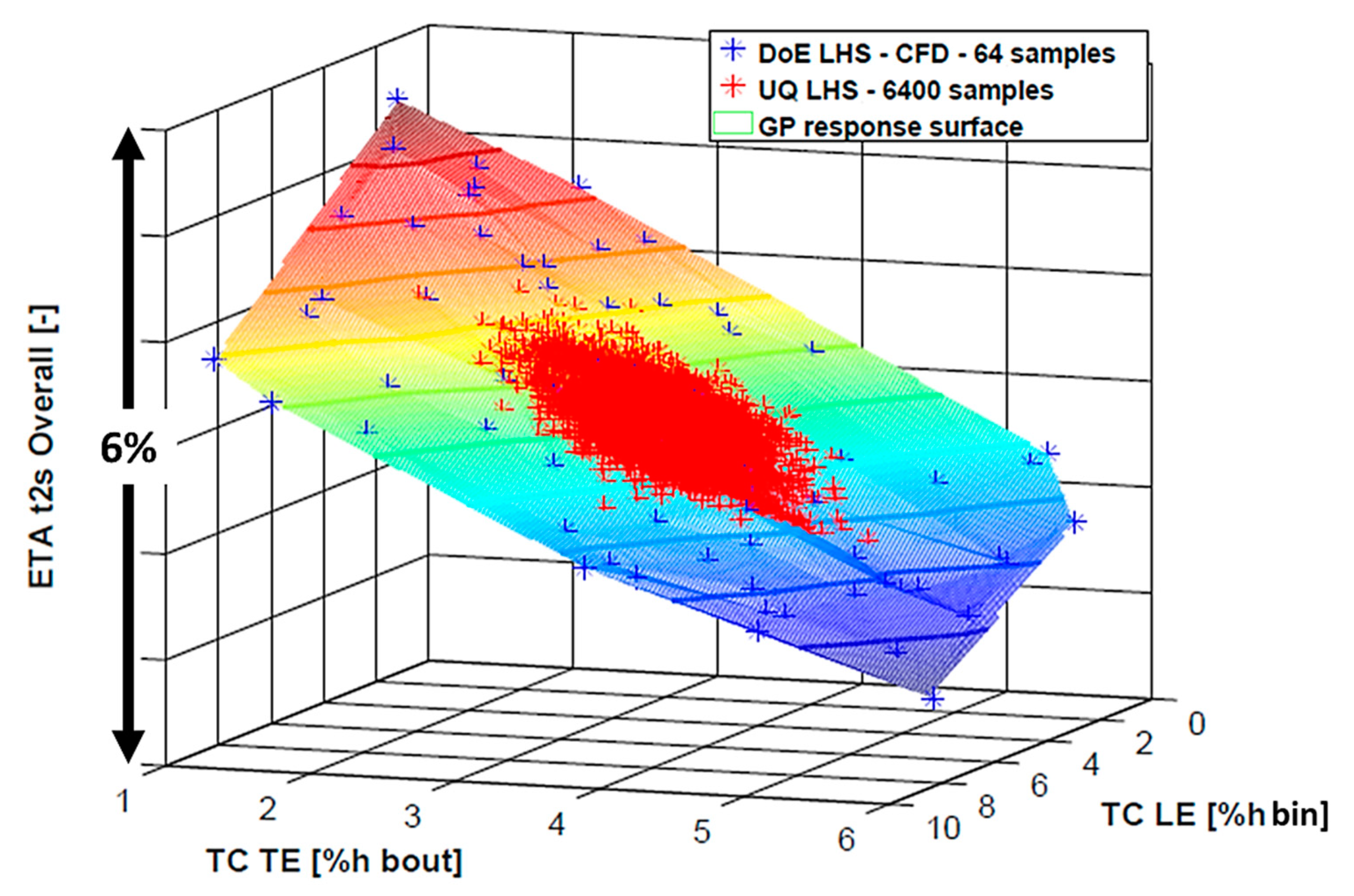
An example of the surrogate generated with the SB-UQ approach is reported in Figure 5 for the overall total to static turbine efficiency (Equation (6)).

Contours have been reported on the response surface to display the overall variation in turbine efficiency as a function of the input parameters (tip clearances at rotor LE and TE). The blue scattered points represent the 64 points of the DoE, which correspond to 64 different combinations of rotor clearance values, i.e., to a database of 64 CFD simulations. This computational effort is necessary to build a reliable surrogate of the CFD model through the RSM (Gaussian Process Equation (7)): the overall efficiency variation inside the DoE is about 6% (see Figure 5 vertical axis).

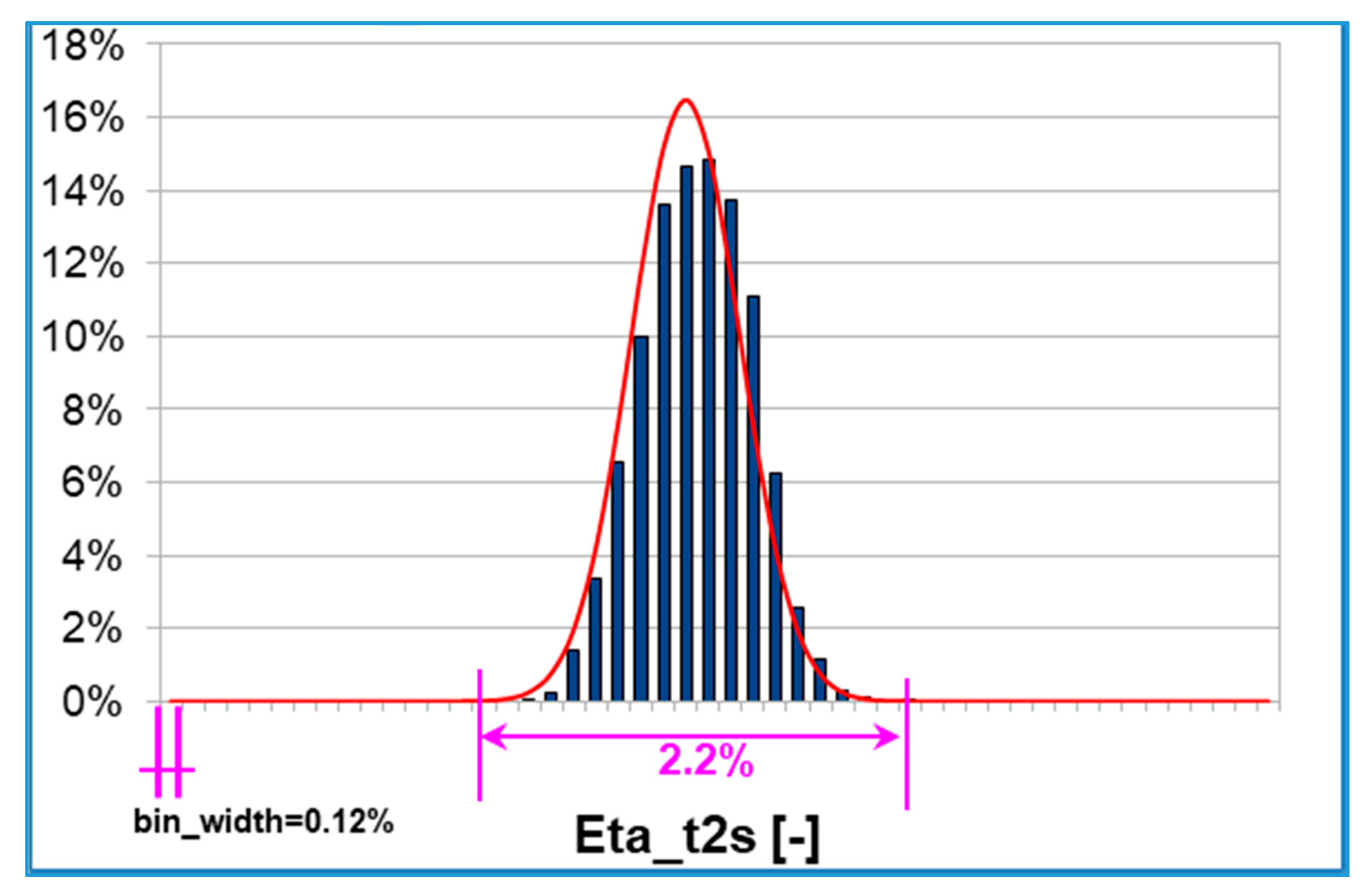
In order to compute the statistics of the response function, the SB-UQ algorithm performs 6400 (2 orders of magnitude greater than the DoE) function evaluations on the meta-model, which are visible in red scatter in Figure 5. The discretized probability distribution of the overall turbine efficiency is plotted in Figure 6, where each bin of the histogram is equal to a 0.12% efficiency difference.

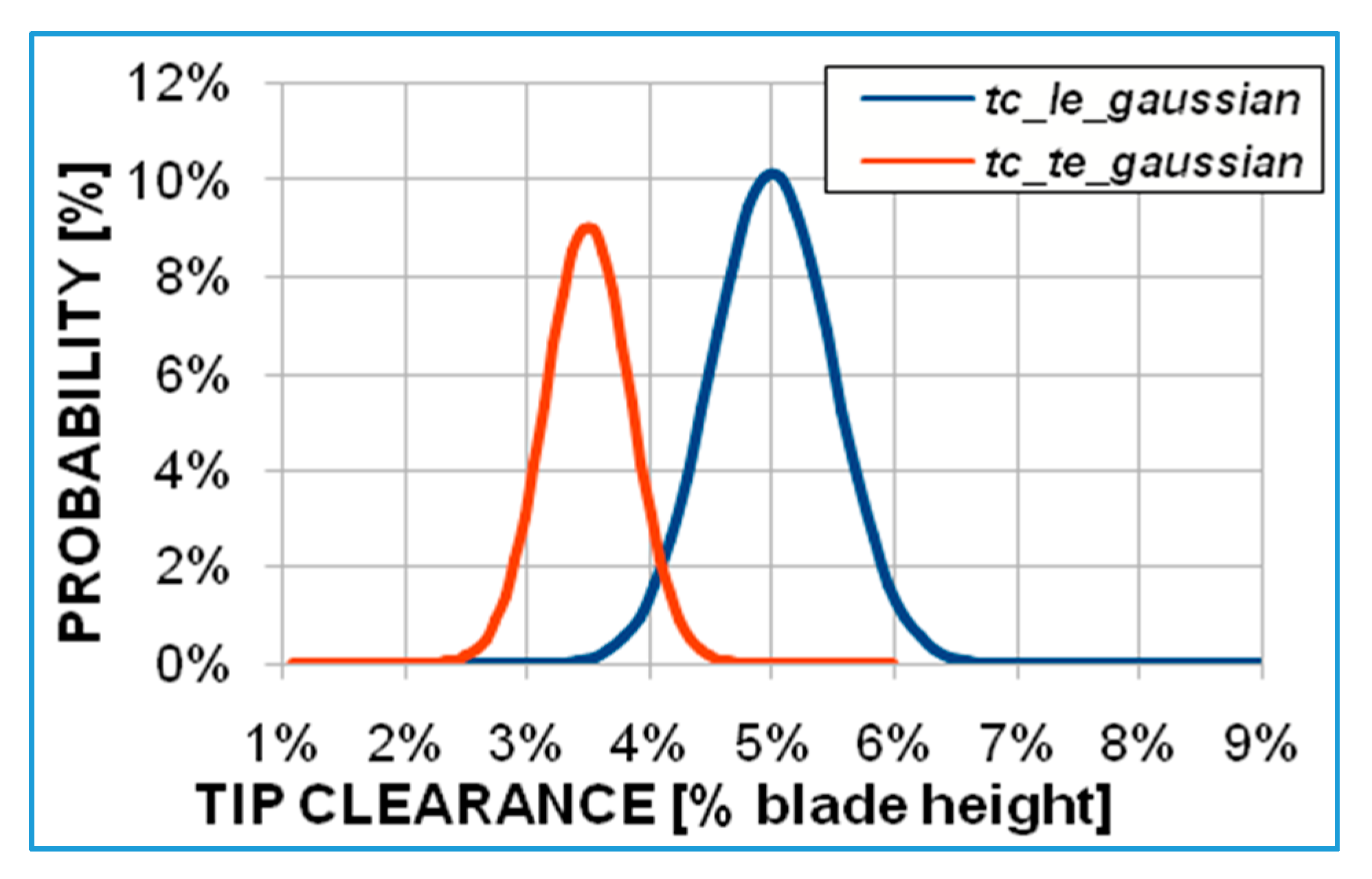
The input uncertainties (Figure 4) correspond to a 2.2% efficiency variation range, where it is possible to fall with non-zero probability. This is a significant outcome: for a fixed turbine operating point subject to rotor tip gap uncertainties (see Table 2) the overall efficiency variability is about 2%. The red line plotted in Figure 6 over the probability bars represents the corresponding Gaussian distribution with the same average and standard deviation of the discretized PDF computed by Dakota.

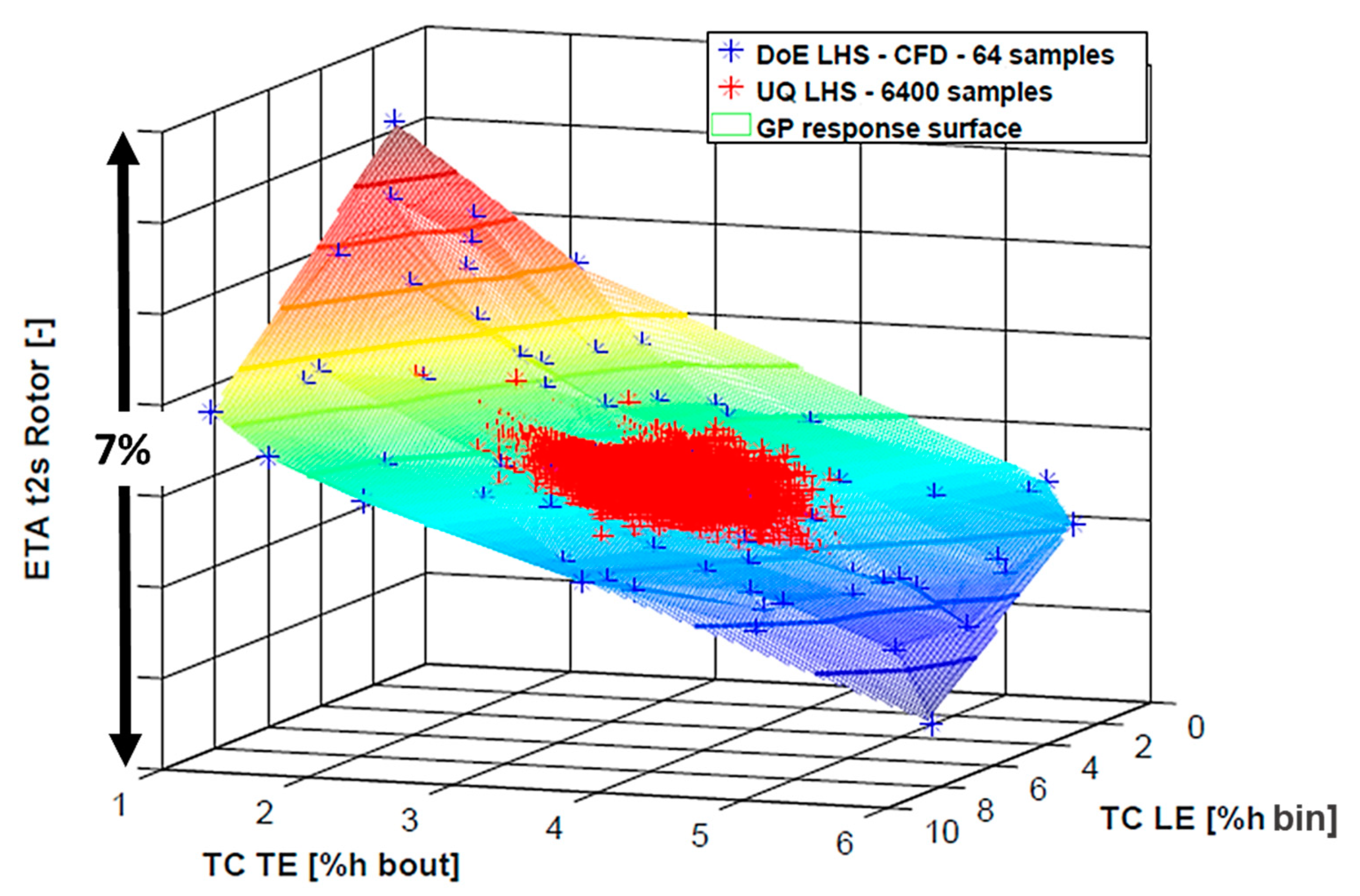
Rotor total to static efficiency (calculated with the rotor expansion ratio $PR{F}_{rotor}$) has a slightly different behavior and a wider variability inside the DoE: about 7% variation as indicated in Figure 7.

The rotor efficiency larger sensitivity (compare Figure 5, Figure 6 and Figure 7) can be explained considering that tip gap variations directly affect the rotor efficiency while the stage efficiency also includes volute and tailpipe losses that tend to hide the effect of tip clearance gap.

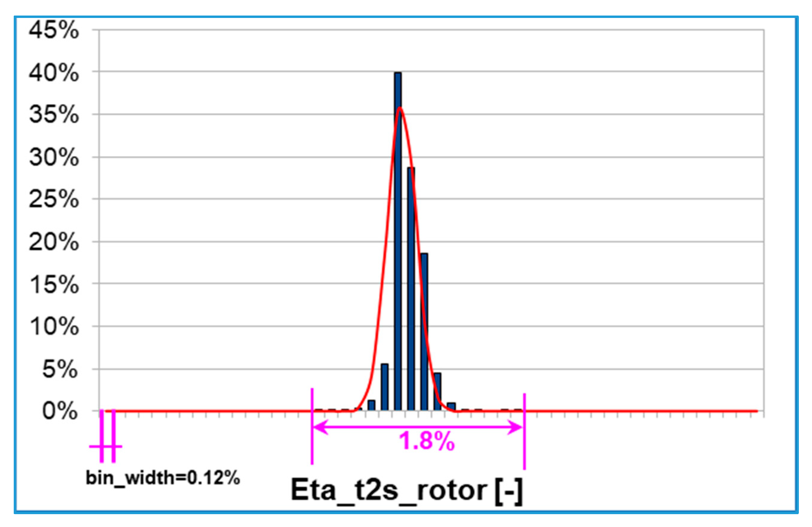
However, the rotor total to static efficiency probability distribution is sharper and less dispersed than the previous one (compare Figure 6, Figure 7 and Figure 8).

Among the statistical quantities provided by the UQ analysis, the Skewness (Equation (13)) and the excess Kurtosis (Equation (14)) are obtained from the following equations:

$$Sk=E\left[{\left(\frac{R_i-{\mu }_i}{{\sigma }_i}\right)}^3\right]\cong \frac{1}{{\sigma }_i{}^3}\left[{\displaystyle \sum }_{k=1}^{N_p}{\left(r_{ik}-{\mu }_i\right)}^3{\omega }_k\right]$$

(13)

$$Ku=E\left[{\left(\frac{R_i-{\mu }_i}{{\sigma }_i}\right)}^4\right]-3\cong \frac{1}{{\sigma }_i{}^4}\left[{\displaystyle \sum }_{k=1}^{N_p}{\left(r_{ik}-{\mu }_i\right)}^4{\omega }_k\right]-3$$

(14)

where ${\mu }_i$ is the mean, ${\sigma }_i$ the standard deviation and E is the expectation operator.

The skewness (Sk) is a measure of the asymmetry of the probability distribution of a real-valued random variable about its mean, while the excess Kurtosis (Ku) describes the shape of a PDF with respect to the Gaussian distribution having Ku = 0.

The corresponding values of these statistics moments are reported in

Table 3. SB-UQ: 3rd and 4th order moment statistics values for rotor and ‘overall’ efficiency.

QoI	Skewness (Sk)	Excess Kurtosis (Ku)
ETA_t2s_Overall	−0.0195	−0.3046
ETA_t2s_Rotor	0.2982	2.3968

and the following considerations can be drawn:

• overall efficiency: comparing the discretized probability with the corresponding Gaussian (Figure 6) it is clear that the distribution is left-skewed (Sk < 0), i.e., the left tail is longer and the mass of the distribution is concentrated on the right of the figure. Moreover, Ku < 0 and the distribution is defined ‘platykurtic’, i.e., it is flatter than the corresponding Gaussian, resulting in thinner tails;
• rotor efficiency: the distribution is right-skewed (Sk > 0) instead, i.e., the right tail is longer and the mass of the distribution is concentrated on the left of the figure. Ku > 0 and the distribution is defined ‘leptokurtic’, i.e., it is sharper than the corresponding Gaussian, resulting in fatter tails.

The difference between rotor and stage efficiency probability distributions can be explained comparing the corresponding response surfaces. In Figure 7 the surface has an inflection at the tip clearance average values. Since the input distributions are Gaussian, the majority of UQ samples falls around the mean values giving a lower variability of the rotor efficiency.

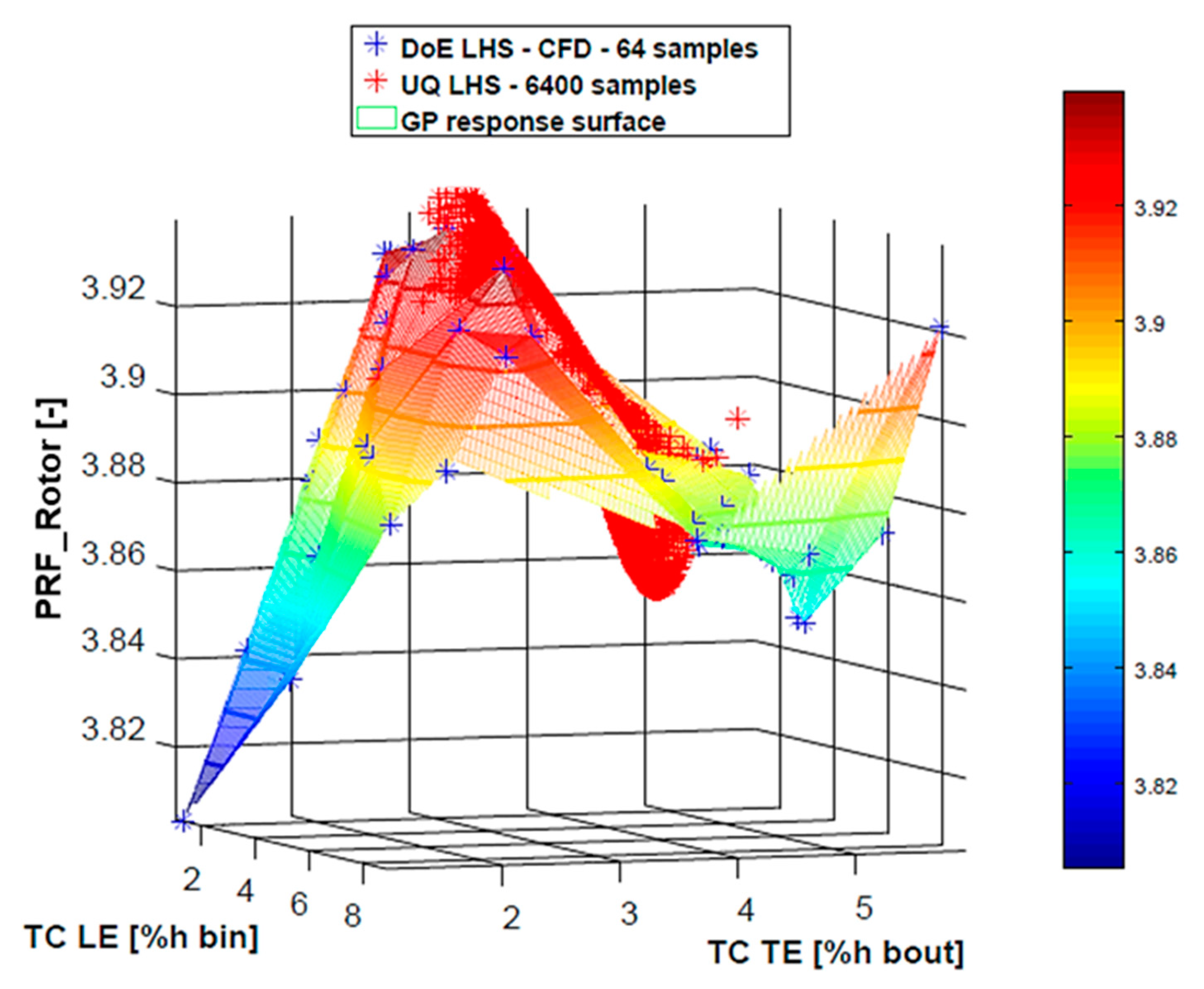
The abovementioned inflection in rotor efficiency response surface is due to the peculiar behavior of the rotor pressure ratio, whose response surface is shown in Figure 9.

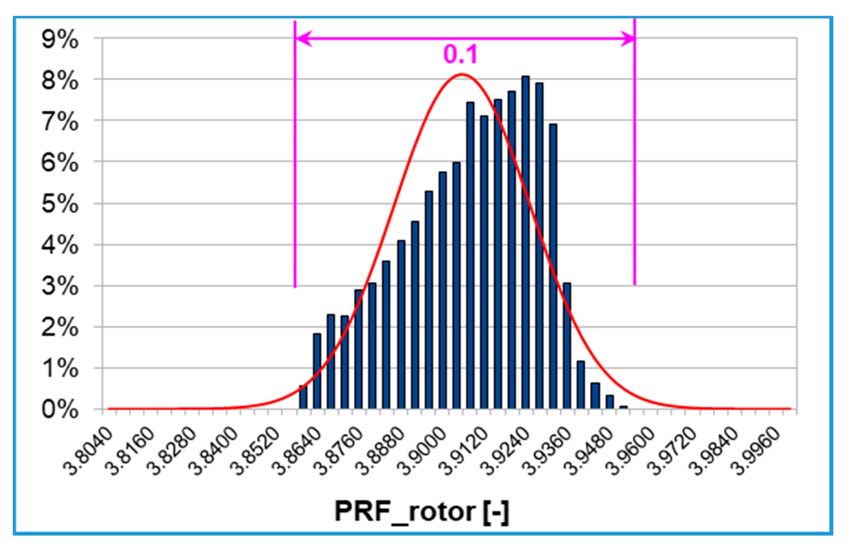
The resulting PDF is displayed in Figure 10 where the input uncertainties correspond to about 0.1 rotor pressure ratio variation range. The rotor pressure ratio probability distribution is almost uniform within this range with the highest peaks at around 8%.

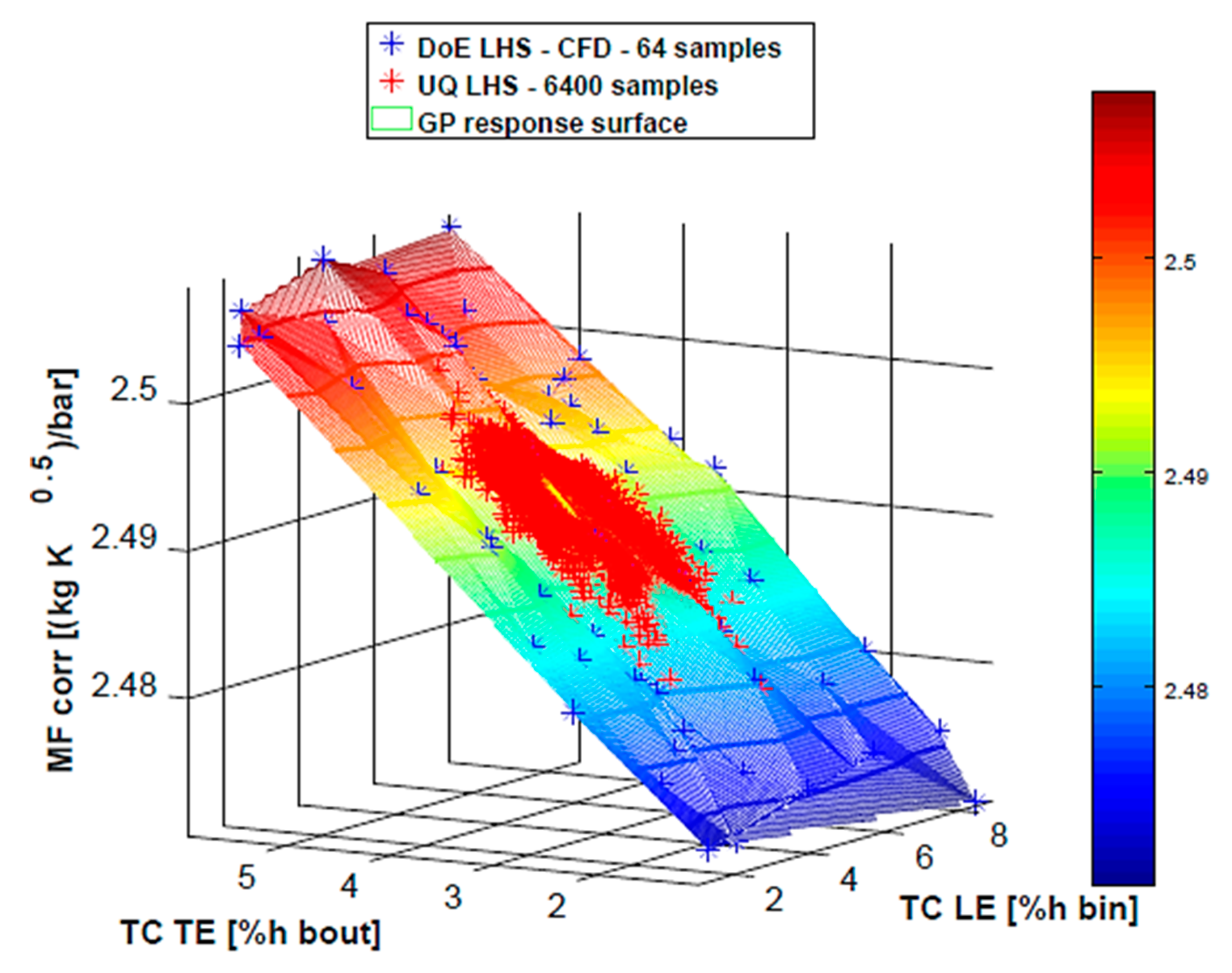
Figure 11 shows the response surface of the mass flow parameter with the dataset points. It is evident from the surface gradient that the tip gap at blade TE has a higher influence on the MFP than the tip gap at the blade LE.

The TE tip clearance reduction (i.e., TE blade tip closer to the shroud) leads to an appreciable lowering of the mass flow parameter, i.e., of the turbine exhaust gas swallowing capacity. This result matches the radial turbines design theory where the aerodynamic blockage in the exducer (final part of the blade) limits the impeller blades number.

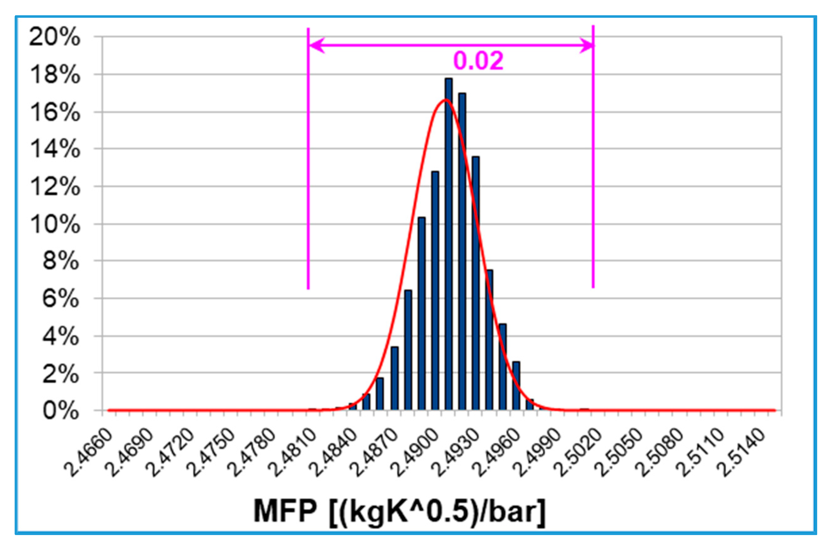
The MFP discretized probability distribution is reported in Figure 12. The 6400 results of the sampling-based UQ algorithm are concentrated in a small range of 0.02 [(kgK^0.5)/bar], equal to 0.8% of the mean value of the distribution. It can be observed that tip gap uncertainties have a limited impact on turbine mass flow, which is slightly affected by TE tip clearance.

6.2. Surrogate Model Validation

The surrogate models given by Dakota’s Surfpack toolset allows to compute diagnostics metrics on the basis of [8]:

1)

simple prediction error with respect to the training data. In this case the points $x_i$ are those used to train the model;

2)

prediction error estimated by cross-validation, when the points $x_i$ are selectively omitted from the build;

3)

prediction error with respect to challenge data, which are supplementary points $x_i$ provided by the user.

The resulting metrics must be interpreted very carefully; in case of interpolatory models, like those used for the surrogate generation, simple prediction error (1) will almost always be zero. The determination coefficient ($R^2$) is meaningful for polynomial models, but less for other model types.

In order to check the meta-model reliability, a cross-validation was performed. At first the k-fold cross-validation is considered: the DoE dataset is divided into k partitions and k meta-models are generated, each excluding the k-th partition of training data. Each surrogate is tested at the points that were excluded for the generation and the user-specified diagnostic metrics are computed with respect to the held-out data [8]. The results obtained from a 4-fold cross-validation are reported in

Table 4. Metrics for 4-fold cross validation of the response surfaces.

Metrics	Eta_ts	Eta_ts rot	PRF rot	MFP [kgK0.5/bar]
Root Mean Squared (RMS)	5.766 × 10−4	1.428 × 10−3	1.794 × 10−2	1.356 × 10−3
Mean Absolute Value (%mean value)	0.08%	0.20%	0.33%	0.04%
Maximum Absolute Value (%mean value)	0.30%	0.97%	1.52%	0.15%

, including the Root Mean Squared, the Mean Absolute Value and the Maximum Absolute Value of the prediction error (calculated between the observed value and the surrogate model prediction for the training data points). The average and maximum absolute values of the prediction error (last two rows of Table 4) are reported in relative percentage form with respect to the corresponding average values of the 64-points DoE.

The results confirm the reliability of the model, with average errors never above 0.5% and maximum errors contained within 1.5%. In addition, the Leave-one-out cross-validation or Prediction Error Sum of Squares (PRESS) was performed. In this special case of k-fold cross-validation the number of partitions is equal to the number of data points. The results given by this analysis are summarized in

Table 5. Metrics for Leave-one-out cross validation (PRESS) of the response surfaces.

Metrics	Eta_ts	Eta_ts rot	PRF rot	MFP [kgK0.5/bar]
Root Mean Squared (RMS)	5.116 × 10−4	1.339 × 10−3	1.738 × 10−2	1.393 × 10−3
Mean Absolute Value (%mean value)	0.07%	0.17%	0.29%	0.04%
Maximum Absolute Value (%mean value)	0.27%	1.03%	1.71%	0.15%

.

The results of Table 5 confirm the outcome of the 4-fold cross validation. The maximum error slightly increases (1.71%) as expected because the number of partitions used to evaluate the statistical quantities corresponds to the number of training points. Maximum errors within 2% are considered acceptable and confirm the validity of the UQ results discussed in Section 6.1. The SB-UQ approach is therefore taken as reference to assess the quality of the PDFs obtained with PCE of different orders.

6.3. PCE: Results Comparison among Different Expansion Orders

The Polynomial Chaos Expansion technique requires the order of expansion of the multivariate polynomial approximation and the polynomial order bounds for each input variable.

The GP algorithm previously used in the Surrogate-based approach (Section 6.1) requests a 2nd order polynomial for the trend function of each response function and the highest total polynomial order of any term in the trend function is 2. However, if no information on the response behavior is available, it is essential to compare the output PDF resulting from different orders of the polynomial expansion. In this paper the results from a 2nd, 3rd and 4th order polynomial expansions are compared, in order to give some guidelines for future applications of UQ approaches on twin scroll radial turbines. The comparison of the overall total to static efficiency discretized PDFs is shown in Figure 13.

It is interesting to note that 2nd and 4th order PDFs are more similar close to the mean value, while 3rd order polynomial expansion PDF differs from the previous ones, with higher probability peaks close to the distributions average value.

If the SB-UQ distribution is taken as reference, the closest is the 4th order expansion, especially taking into account the central bars, related to higher probability levels. Looking at the absolute maximum probability difference between the PCE and the SB-UQ distributions (

Table 6. Overall efficiency maximum absolute probability differences from SB-UQ approach.

Eta_t2s MAX prob. Diff. PCE—SB-UQ
2nd	3rd	4th
1.22%	2.22%	0.83%

), the 2nd and 4th differs only for 0.4%.

At this point the question is legitimate: is it worth doing 16 CFD simulations instead of 4 (minimum required number for 4th and 2nd order PCE respectively) for such a small improvement? The answer to this question can be given considering the assembly of all response functions.

One interesting result is that again the 3rd order PCE is the more distant from SB-UQ probability prediction. Figure 13 and Table 6 highlight an interesting fact: with the 2nd order PCE it is possible to get an overall efficiency probability distribution which differs from the SB-UQ by a maximum of 1%.

The PCE technique allows to obtain optimal probability predictions with a much lower computational effort: from 64 CFD simulations required for the meta-model to only 4 simulations for the 2nd order multivariate polynomial chaos expansion.

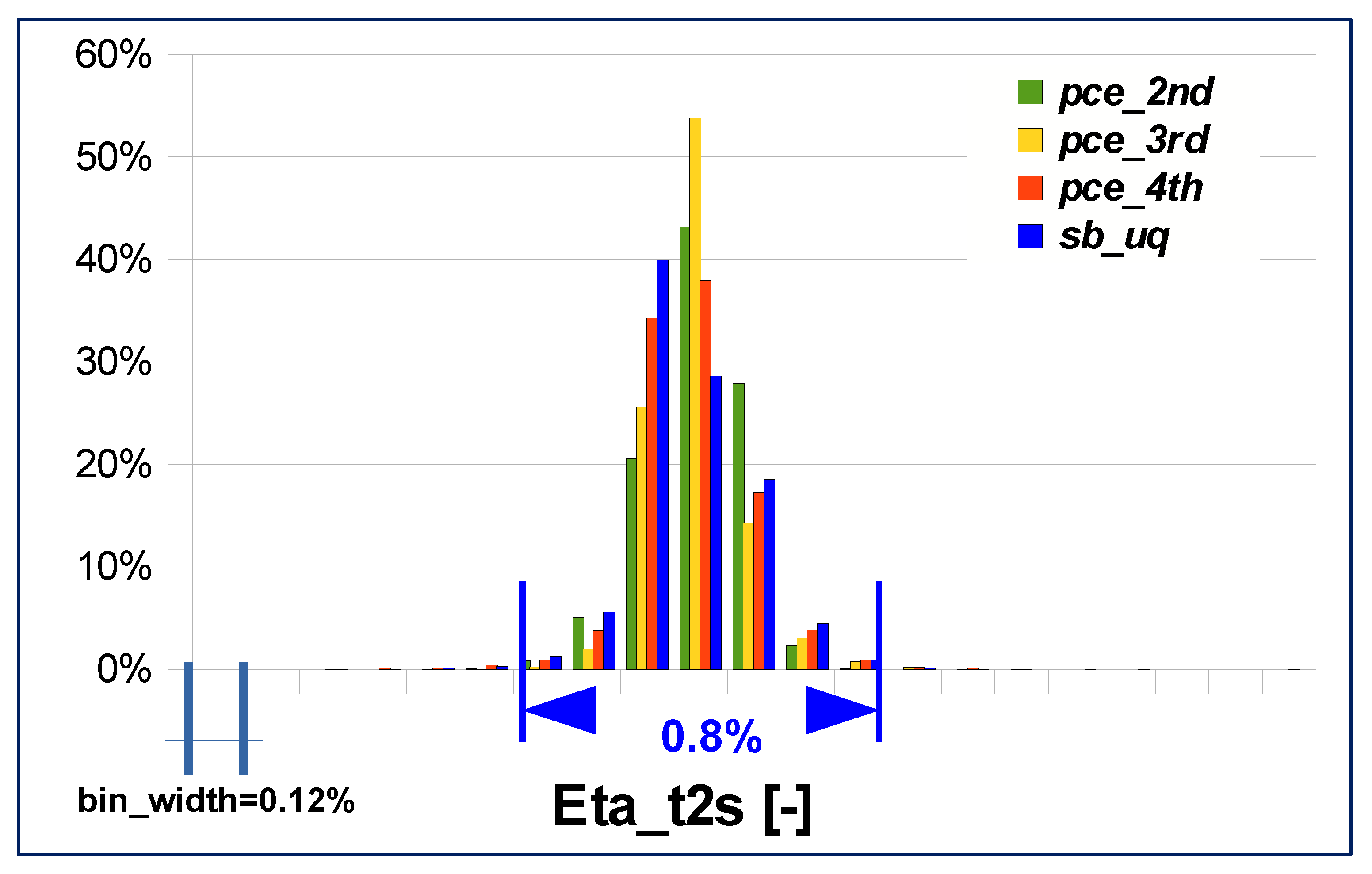
The rotor total to static efficiency is plotted in Figure 14. It can be noted that, as the overall efficiency, the 3rd order polynomial expansion is the sharpest distribution.

Lower order expansions (2nd and 3rd) show more concentrated probabilities around the PDFs mean value, while 4th order and SB-UQ have a larger probability dispersion.

The difference between the 2nd and 4th order polynomial PDFs is larger in this case as reported in

Table 7. Rotor efficiency maximum absolute probability differences from SB-UQ approach.

Eta_t2s_rot MAX prob. Diff. PCE—SB-UQ
2nd	3rd	4th
19.39%	25.13%	9.31%

; the 2nd order maximum probability difference from the SB-UQ is twice than with the 4th order PCE. The larger difference found in the rotor efficiency probability distributions would require the adoption of a 4th order PCE.

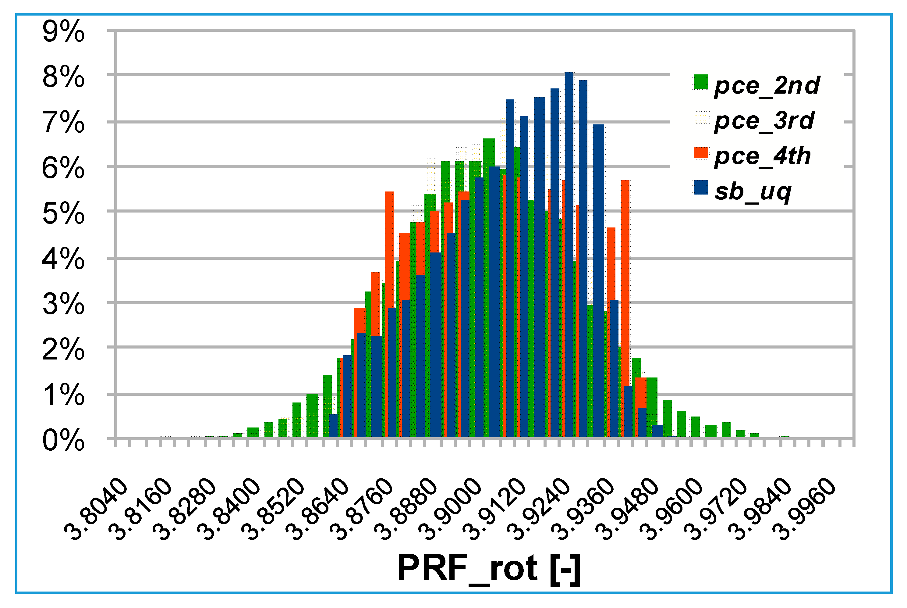
All the probability distributions for the rotor pressure ratio from the PCE differ in shape from the reference; moreover, lower orders (2nd and 3rd) have a larger dispersion within the dataset as shown in Figure 15.

The maximum percentage difference from the surrogate model is always around 3–4%, as confirmed by

Table 8. Rotor pressure ratio maximum absolute probability differences from SB-UQ approach.

PRF_rot MAX prob. Diff. PCE—SB-UQ
2nd	3rd	4th
4.52%	3.25%	3.98%

. However, it must be stressed that the 4th order PCE is the one that qualitatively best fits the results of the SB-UQ.

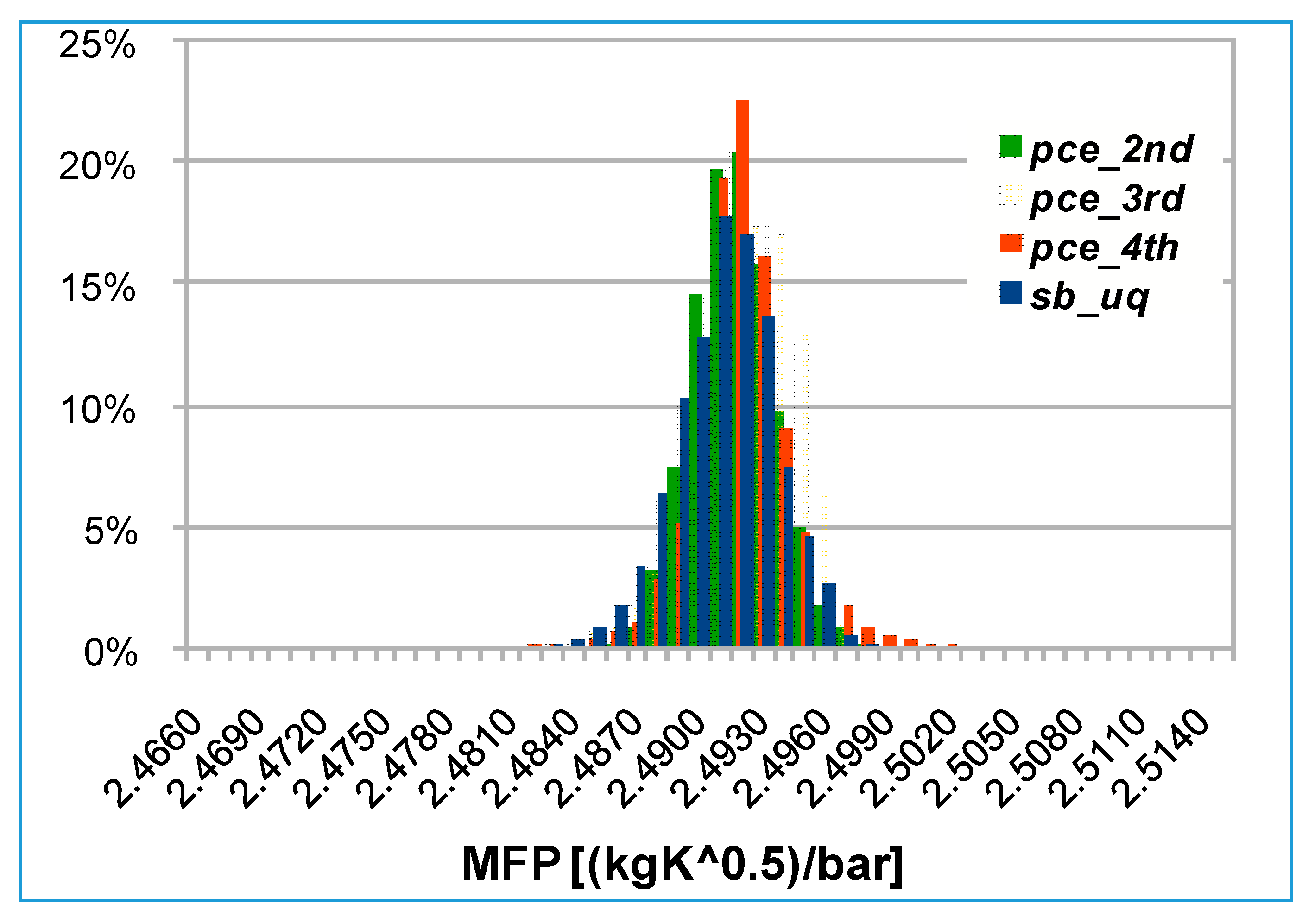
Finally, the mass flow parameter is considered: PDFs are almost entirely contained in a range of amplitude equal to 0.8% of the average value of the distribution (see Figure 16). Analyzing the data in

Table 9. Mass flow parameter maximum absolute probability differences from SB-UQ approach.

MFP MAX prob. Diff. PCE—SB-UQ
2nd	3rd	4th
5.58%	9.59%	3.34%

it can be concluded that quantitatively the 4th order PCE is the solution that best approximates the probability distribution of the surrogate-based approach with a maximum error of about 3%.

7. Conclusions

The application of the UQ analysis to a radial turbine with the introduction of uncertainties in the tip clearance gaps at blade LE and TE has demonstrated the capabilities and large potential of these numerical techniques for turbomachinery design purposes. The effects of rotor tip gap uncertainty have been quantified and overall results from radial turbine design practice has been confirmed. Two approaches have been developed and compared: response surface vs. polynomial chaos. A validation method has been developed and applied to the reference case of response surface UQ method. The use of polynomial chaos is very attractive because it requires a much lower number of individuals in the CFD database but the order of the polynomial strongly affects the final distributions in the UQ analysis. The best polynomial order for the present application case has been obtained and validated using the response surface method as reference.

The final target of this analysis is to provide a quantitative indication to the designer of how much the performance obtained preliminarily through a CFD simulation may vary due to operational geometric uncertainties due to rotor tip clearances.

The designer can extract realistic information on the performance attainable in a given working point and can correlate the simulated data with the actual performance.

References

1. Montomoli, F.; Carnevale, M.; D’Ammaro, A.; Massini, M.; Salvadori, S. Uncertainty Quantification in Computational Fluid Dynamics and Aircraft Engines; Springer: Berlin, Germany, 2019. [Google Scholar]
2. Montomoli, F.; Massini, M.; Salvadori, S. Geometrical uncertainty in turbomachinery: Tip gap and fillet radius. Comput. Fluids 2011, 46, 362–368. [Google Scholar] [CrossRef]
3. Satish, T.N.; Murthy, R.; Singh, A.K. Analysis of uncertainties in measurement of rotor blade tip clearance in gas turbine engine under dynamic condition. J. Aerosp. Eng. 2014, 228, 652–670. [Google Scholar] [CrossRef]
4. Krishnababu, S.K.; Newton, P.J.; Dawes, W.N.; Lock, G.D.; Hodson, H.P.; Hannis, J.; Whitney, C. Aerothermal Investigations of Tip Leakage Flow in Axial Flow Turbines—Part I: Effect of Tip Geometry and Tip Clearance Gap. ASME J. Turbomach. 2009, 131, 11006. [Google Scholar] [CrossRef]
5. Cravero, C.; De Domenico, D.; Ottonello, A. Numerical simulation of the performance of a twin scroll radial turbine at different operating conditions. Hindawi Int. J. Rotating Mach. 2019, 2019, 5302145. [Google Scholar] [CrossRef]
6. Cravero, C.; Macelloni, P.; Briasco, G. Three-dimensional design optimization of multi stage axial flow turbines using a RSM based approach. In Proceedings of the ASME Turbo Expo 2012, Copenhagen, DK, USA, 11–15 June 2012. [Google Scholar]
7. Cravero, C. Turbomachinery design optimization based on metamodels. In Proceedings of the 4th Inverse Problems Design and Optimization Symposium IPDO-2013, Albi, France, 26–28 June 2013; ISBN 979-10-91526-01-2. [Google Scholar]
8. Adams, B.M.; Ebeida, M.S.; Eldred, M.S.; Jakeman, J.D.; Swiler, L.P.; Stephens, J.A.; Vigil, D.M.; Wildey, T.M. Dakota: A Multilevel Parallel Object-Oriented Framework for Design Optimization, Parameter Estimation, Uncertainty Quantification, and Sensitivity Analysis: Version 6.8 User’s Manual; Technical Report SAND2014-4633; Sandia National Laboratories: Albuquerque, NM, USA, 2018.
9. Cravero, C.; De Domenico, D.; Ottonello, A. Uncertainty Quantification Approach on Numerical Simulation for Supersonic Jets Performance. Algorithms 2020, 13, 130. [Google Scholar] [CrossRef]
10. Cravero, C.; La Rocca, M.; Ottonello, A. Performance Characterization of a Twin Scroll Volute for Turbocharging Applications. In Proceedings of the ASME Turbo Expo 2018: Turbomachinery Technical Conference and Exposition, Oslo, Norway, 11–15 June 2018; ASME Paper GT2018-75522. p. V02BT44A010. [Google Scholar]
11. Romagnoli, A.; Martinez-Botas, R.F.; Rajoo, S. Steady state performance evaluation of variable geometry twin-entry turbine. Int. J. Heat Fluid Flow 2011, 32, 477–489. [Google Scholar] [CrossRef]
12. Cravero, C.; De Domenico, D.; Ottonello, A. Investigation on the degree of reaction in twin scroll radial turbines at different operating conditions for turbocharging applications. In Proceedings of the ASME Turbo Expo 2019: Turbomachinery Technical Conference and Exposition, ASME Paper GT2019-90285, ASME Turbo Expo, Phoenix, AZ, USA, 17–21 June 2019. [Google Scholar]
13. Raetz, H.; Kammeyer, J.; Natkaniec, C.K.; Seume, J.R. Numerical Investigation of Aerodynamic Radial and Axial Impeller Forces in a Turbocharger. In Proceedings of the ASME Turbo Expo 2011: Turbomachinery Technical Conference and Exposition, ASME Turbo Expo, Vancouver, BC, Canada, 6–10 June 2011. ASME Paper GT2011-46. [Google Scholar]
14. Lüddecke, B.; Nitschke, P.; Dietrich, M.; Filsinger, D.; Bargende, M. Unsteady thrust force loading of a turbocharger rotor during engine operation. In Proceedings of the ASME Turbo Expo 2015: Turbomachinery Technical Conference and Exposition, ASME Turbo Expo, Montreal, QC, Canada, 15–19 June 2015. ASME Paper GT2015-43559. [Google Scholar]
15. Cavazzuti, M. Optimization Methods: From Theory to Design-Scientific and Technological Aspects in Mechanics; Springer: Berlin, Germany, 2013. [Google Scholar]
16. Cressie, N. Statistics of Spatial Data; John Wiley and Sons: New York, NY, USA, 1991. [Google Scholar]
17. Koehler, J.R.; Owen, A.B. Computer experiments. In Handbook of Statistics; Ghosh, S., Rao, C.R., Eds.; Elsevier Science: New York, NY, USA, 1996; Volume 13. [Google Scholar]
18. Ghanem, R.; Red-Horse, J.R. Propagation of probabilistic uncertainty in complex physical systems using a stochastic finite element technique. Physica D 1999, 133, 137–144. [Google Scholar] [CrossRef]
19. Ghanem, R.G.; Spanos, P.D. Stochastic Finite Elements: A Spectral Approach; Springer-Verlag: New York, NY, USA, 1991. [Google Scholar]
20. Askey, R.; Wilson, J. Some basic hypergeometric polynomials that generalize jacobi polynomials. Mem. Am. Math. Soc. Ams Provid. RI 1985, 319. [Google Scholar] [CrossRef]
21. Adams, B.M.; Bohnhoff, W.J.; Dalbey, K.R.; Eddy, J.P.; Eldred, M.S.; Gay, D.M.; Haskell, K.; Hough, P.D.; Swiler, L.P. Dakota, a Multilevel Parallel Object-Oriented Framework for Design Optimization, Parameter Estimation, Uncertainty Quantification, and Sensitivity Analysis: Version 6.8 Theory Manual; Technical Report SAND2014-4253; Sandia National Laboratories: Albuquerque, NM, USA, 2018.
Figure 1. Unstructured grid detail on the two volute branches. In magenta the volute outlet section.
Fluids 05 00114 g001
Figure 2. Rotor channel structured mesh with volume mesh cut plane (yellow).
Fluids 05 00114 g002
Figure 3. CFD model.
Fluids 05 00114 g003
Figure 4. Input Probabilities (discrete PDF integrals).
Fluids 05 00114 g004
Figure 5. SB-UQ: overall efficiency response surface and samples.
Fluids 05 00114 g005
Figure 6. SB-UQ: overall efficiency probability bars (in blue) and related Gaussian trend (red line).
Fluids 05 00114 g006
Figure 7. SB-UQ: rotor efficiency response surface and samples.
Fluids 05 00114 g007
Figure 8. SB-UQ: rotor efficiency probability bars (in blue) and related Gaussian trend (red line).
Fluids 05 00114 g008
Figure 9. SB-UQ: rotor pressure ratio response surface and samples.
Fluids 05 00114 g009
Figure 10. SB-UQ: rotor pressure ratio probability bars (blue) and related Gaussian trend (red line).
Fluids 05 00114 g010
Figure 11. SB-UQ: mass flow parameter response surface and samples.
Fluids 05 00114 g011
Figure 12. SB-UQ: mass flow parameter probability bars (blue) and related Gaussian trend (red line).
Fluids 05 00114 g012
Figure 13. PCE vs. SB-UQ: overall efficiency probability distributions coming from different polynomial orders
Fluids 05 00114 g013
Figure 14. PCE vs. SB-UQ: rotor efficiency probability distributions coming from different polynomial orders.
Fluids 05 00114 g014
Figure 15. PCE vs. SB-UQ: rotor pressure ratio probability distributions coming from different polynomial orders.
Fluids 05 00114 g015
Figure 16. PCE vs. SB-UQ: mass flow parameter probability distributions coming from different polynomial orders.
Fluids 05 00114 g016