Abstract
A new Partially Averaged Navier-Stokes (PANS) bridging model is derived from existing and PANS formulations. The model behaves like the PANS model near rigid walls and like the PANS model away from walls. The new model is tested using well-known benchmark problems; a backward-facing step representing wall-bounded flows, and a circular cylinder representing free shear flows. Our results are compared to existing experimental data and previous simulation results using PANS and PANS . The comparisons show our model to be superior at predicting velocity profiles in both flows. In addition, Reynolds stress predictions are also shown to improve.
1. Introduction
The desire for inexpensive unsteady simulations of turbulent flows has led to the development of numerous modeling methods which aim to give accurate solutions at a reasonable computational cost. One of the earliest methods, the Unsteady Reynolds Averaged Navier-Stokes (URANS) or Very Large Eddy Simulation (VLES), is inexpensive but unable to resolve the random fluctuations associated with turbulent flows [1]. However, when used in free shear flows with good grid resolution, it can provide useful information about the large-scale structures and in particular the shedding frequency. Certainly, the most accurate method for capturing the physics of unsteady flows is Direct Numerical Simulation (DNS) [2]. In DNS, the full Navier-Stokes equations are solved with no simplifying assumptions. However, this comes at a very high computational cost and is limited to low Reynolds number flows. This is a big drawback since most flows of engineering interest have a high Reynolds number. In order to overcome the Reynolds number limitation of DNS, the Kolmogorov hypothesis [3] is used to take advantage of the universality of the small scales of turbulence at high Reynolds numbers. Based on that, Kolmogorov proposed the first two-equation eddy viscosity model [4] and opened the door for many more to come later. The scale separation operation proposed by Kolmogorov [3] is the foundation for a new method called Large Eddy Simulation (LES). In LES the smallest scales of motion are modeled, while the large scales are fully resolved [5,6,7]. This space filtering operation reduces the computational cost when compared to DNS. However, the computational cost remains high at high Reynolds numbers and hence the need for even cheaper methods.
In recent years, a new family of methods has emerged. These methods known as Hybrid RANS/LES take advantage of the vast knowledge developed in RANS to bridge the gap in the wavenumber space with LES, thus the often-used name of Bridging models [8,9]. One such method is the Detached Eddy Simulation (DES) of Squires et. al. [10]. In DES, the wall region is modeled with RANS while LES is used away from viscous walls. There are several variants of DES in the literature [11,12,13], each claiming an improvement over the original model. Another bridging method is the Partially Averaged Navier-Stokes (PANS) due to Girimaji [14]. PANS can be used to smoothly transition from URANS to DNS by changing the values of some resolution control parameters and refining the grid. Two PANS models exist in the literature [15,16], one based on the Jones and Launder RANS model [17] and the other based on the Wilcox RANS model [18]. There are several other Hybrid RANS/LES models in the literature [19,20], each claiming a specific benefit.
In this paper, we propose a new PANS model based on the and versions of PANS and using the Menter blending idea introduced in RANS [21]. Our goal is to take advantage of the near-wall benefits of PANS and the far field benefits of PANS with the overarching goal of improving predictions from the resulting model. The remainder of the paper is organized as follows; the mathematical model is derived in Section 2, followed by the results and discussion in Section 3, and the concluding remarks are given in Section 4.
2. Mathematical Model and Method of Solution
The unsteady, incompressible forms of the Navier-Stokes equations are given by
where is the instantaneous velocity and is the pressure. The Poisson equation relates pressure and velocity through
The flow variables are filtered or partially averaged, and the resulting resolved variables are given by
The velocity and pressure fields are related to the resolved and unresolved variables by
Introducing Equations (3) and (4) into Equations (1) and (2) leads to the Partially Averaged Navier-Stokes (PANS) equations
The filtering process introduces sub-filter scale stresses (SFS) which lead to a closure problem in the PANS equations. The SFS are given by the generalized central second moment of the instantaneous velocities
The pressure fluctuation p’ in Equation (4) is solved with the following Poisson Equation [14]
Modeling of the SFS stress is performed by the extension of Reynolds Averaged Navier Stokes (RANS) turbulence models to PANS. In the PANS formulation, the ratio of the unresolved to the total turbulent quantities are specified by the PANS resolution control parameters. The subscript u is used to signify unresolved quantities
In Equation (9), is the turbulent kinetic energy, the turbulent dissipation and the turbulent frequency. The resolution control parameters vary between 0 and 1 depending on the flow conditions and grid resolution. When using RANS, the values of the resolution control parameters are set to 1, whereas in DNS the values should be set to 0; i.e., all scales are resolved. This scale resolution cannot be achieved without an appropriate grid resolution based on the Reynolds number. In this paper, the values used are taken from the literature for comparisons. The grid resolution should be appropriate for the chosen values. The reader is referred to prior work for more details on these parameters.
Starting with the PANS formulation given by [14]
The turbulent dissipation rate, and the turbulent production, Pu, are given by
The resolution control parameters are used to vary the PANS model constants from the RANS constants. Only one constant must be changed in the PANS formulation
To bridge the and models, the -equation will be rewritten in terms of ω using Equation (12). To this end, the time derivative and gradient of the turbulent dissipation can be written in terms of the turbulent kinetic energy and frequency
The terms on the right-hand side of the dissipation equation, Equation (10), can also be rewritten as
Rewriting the full transformed equation and rearranging the terms gives
The first bracketed term on the left-hand side is equal to zero by virtue of Equations (11) and (12), and using
leads to the model obtained from the transformed
The model constants are given by
where . The original PANS is given by [16]
where the constants are
where . The unresolved eddy viscosity of the and PANS models can be related to one another through
The two models are bridged by multiplying the original PANS with a blending function F and the PANS obtained from the modified PANS by (1 − F) and adding the two
The blending function is given by
with
where is the distance from the wall and is the kinematic viscosity. The blended constants are given by
The model described above was then implemented in the open-source software known as OpenFOAM [22]. The grid generation was performed using either the built-in tool, blockMesh, within OpenFOAM; or using Gmesh [23] outside of OpenFOAM. All these tools are readily available for download from the web. Depending upon the size of the grid used for a given problem, a single processor or a multi-processor machine was used. For the two problems presented in this paper, computations can take hours to a few days depending on machine availability. The computations presented here are time-dependent and hence require a long integration time to achieve a statistically steady state. The boundary conditions used are the standard inflow-outflow, far field, and symmetry in the streamwise, vertical, and spanwise directions, respectively (see Reference [24] for more details).
3. Results and Discussion
Simulations have been performed on wall-bounded and free shear flows to validate the model. A backward facing step is used for the wall-bounded flow and a circular cylinder is used for the free shear flow. Experimental data [25,26] and previous PANS simulation results [14,15,16] have been used for comparisons.
3.1. Wall-Bounded Flows: Backward-Facing Step
Despite its simple geometry, a backward-facing step flow presents a challenging problem for turbulence modeling and is considered a standard test case for turbulence model validation. The relevant physics include boundary layer separation from the edge of the step, shear layer reattachment downstream, a recirculation region near the step, and accompanying turbulent motion of the fluid. For the backward-facing step, the size of the computational domain is 10H × 5H × 3H in the region upstream of the step and 20H × 6H × 3H in the region downstream of the step, where the step height is H and the dimensions are given in the streamwise, normal, and spanwise directions, respectively. A 6H wide computational domain was used to examine the effect of the spanwise dimension on the results. The domain spanning 6H has equivalent streamwise and normal dimensions to the domain spanning 3H. The Reynolds number based on the step height is 37,500. The domain is discretized with a structured mesh of hexahedral elements, as shown in Figure 1. For the 3H domain, the inlet region upstream of the step has 92 × 81 × 60 cells. Downstream of the step, the grid is 230 × 168 × 60 in the streamwise, normal, and spanwise directions, respectively. The 6H domain has 120 cells in the spanwise direction. The grid resolution gives dimensionless wall-based distances of y+ < 1, and z+ < 60 throughout the whole domain. The streamwise resolution varies from x+ < 1 at the step to a maximum of x+ < 140 at 5H and farther downstream.
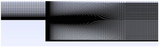
Figure 1.
View of the backward step mesh near the step.
In wall-bounded flows such as the backward-facing step, resolving the turbulence dissipation near the wall becomes critical for accurate prediction of flow quantities. Therefore, the value of should be less than 1 and it is set to 0.667 as in prior references. In addition, the value of is fixed at 0.2 indicating a high resolution of the turbulent kinetic energy. The mean turbulent kinetic energy, Reynolds stress, and velocity profiles are compared with experimental data and previous and PANS results at several locations downstream of the step. Following the available experimental data, the mean turbulent kinetic energy neglects the spanwise fluctuation contribution and is calculated using .
Before comparing the results of our new model to those in the literature and experimental data, we embark on a domain size study, namely the lateral extent of the computational domain. Prior numerical studies [15] used three step heights (3H) as the lateral dimension. However, questions arose as to whether the two-point correlation of the fluctuating velocity decayed to zero within the computational domain. To this end, another simulation was carried out with a computational domain size doubled in the lateral direction, i.e., 6H. Two-point correlations of the velocity fluctuations across the span of the domain were calculated for both the 3H and 6H cases. The sampling location was at the height of the step (1H from the lower wall) and 1H downstream of the step. Figure 2 gives the two-point correlation for the x-component of the streamwise velocity fluctuation. The figure shows that the two-point correlation decays rapidly to zero away from the center for both the 3H and 6H domains. This indicates that the 3H-wide computational domain is sufficient to capture the relevant physics. To further confirm that, comparisons of the mean velocity profiles at a downstream location of x/H = 5 are shown in Figure 3. Little to no difference between the velocity profiles is shown by the figure. Similarly, the mean kinetic energy profile at the same downstream location is shown in Figure 4. In this case, small differences are shown due to the proximity of the reattachment point. Similar results are obtained for the mean Reynolds stress profile, Figure 5. Based on these results, the 3H-wide computational domain is deemed sufficient and is used for the remainder of this paper.

Figure 2.
Two-point correlation of at 1H downstream of the step
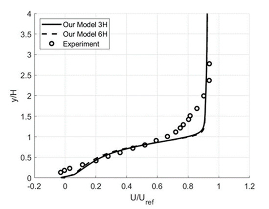
Figure 3.
Mean velocity profile at from the step .
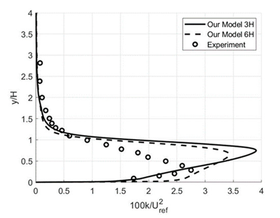
Figure 4.
Mean kinetic energy profiles at from the step
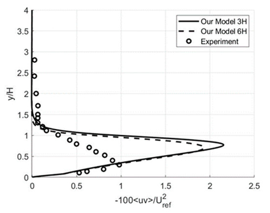
Figure 5.
Mean Reynolds stress profiles at from the step
The performance of the proposed model is compared to experimental data [25] and previous and PANS results [14,15,16]. As mentioned in the previous section, our results are obtained using a computational domain spanning 3H in width. The PANS results [15] were obtained for . Figure 6 and Figure 7 show the mean velocity profiles at x/H of 5H and 6H downstream of the step. The figures show that the new model gives the best agreement with experimental data. In addition, the predictions of the new model fall between the previous and PANS models’ results, which is expected. The downstream locations chosen are near the reattachment point.
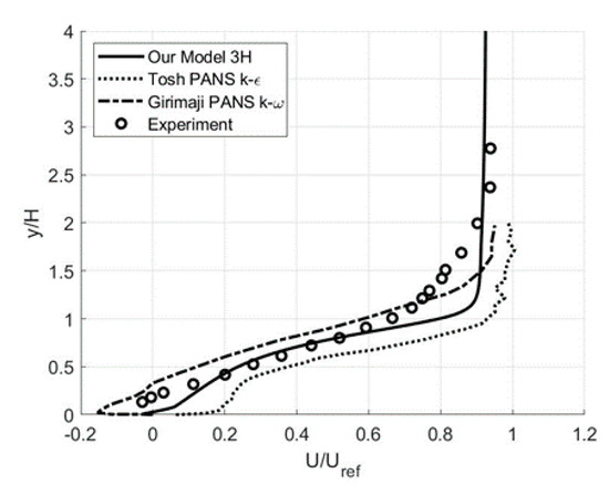
Figure 6.
Mean velocity profiles at x/H = 5 from the step .
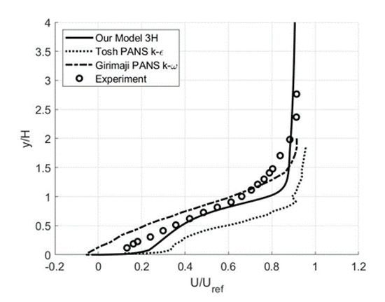
Figure 7.
Mean velocity profiles at x/H = 6 from the step
The mean turbulent kinetic energy profiles at x/H of 2 and 5 are given in Figure 8 and Figure 9. At both locations, our model predictions are in better agreement with the experimental data.
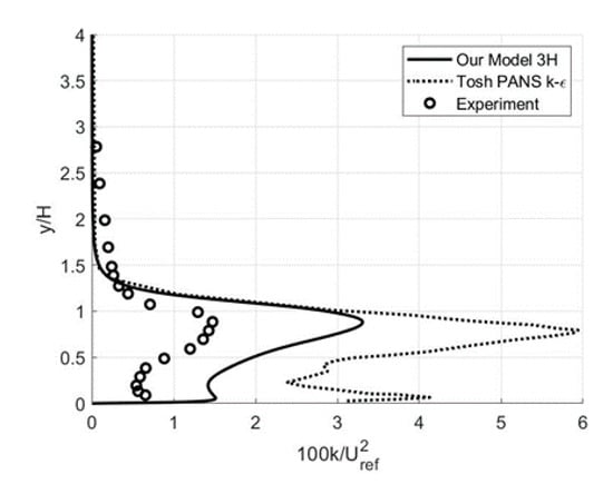
Figure 8.
Mean kinetic energy profiles at x/H = 2 from the step (
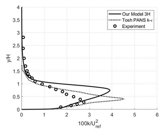
Figure 9.
Mean kinetic energy profiles at x/H = 5 from the step (
The mean Reynolds stress profiles are given in Figure 10 and Figure 11 at the downstream locations of x/H = 2 and 5 from the step. Near the step, x/H = 2, our model predictions are in better agreement with experimental data. Away from the step, x/H = 5, our model follows the experimental data closely near the wall but overpredicts the peak and its location.
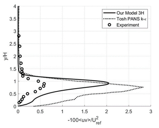
Figure 10.
Mean Reynolds stress profiles at x/H = 2 from the step
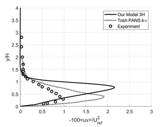
Figure 11.
Mean Reynolds stress profiles at x/H = 5 from the step
Figure 12 shows the Q-criterion iso-contours colored by velocity, which illustrates the turbulent structures shed from the step of Equation (33). The blue color indicates low velocities, and the reddish color indicates higher velocities. As expected, the blue color dominates just downstream of the step due to the recirculation zone.
where is vorticity and is the rate of strain.
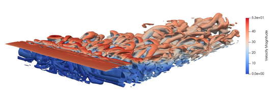
Figure 12.
Q-criterion iso-contours colored by velocity for .
3.2. Free-Shear Flows: Circular Cylinder
The flowfield around a circular cylinder is characterized by strong vortex shedding downstream of the cylinder. The size of the computational domain is 30D × 30D × 3D, where D is the diameter of the cylinder, and the dimensions are in the streamwise, normal, and spanwise directions, respectively. A coarse mesh and a fine mesh are used for the simulations. The coarse mesh consists of 240 × 320 × 48 cells and the fine mesh consists of 300 × 360 × 54 cells in the radial, angular, and spanwise directions, respectively. The coarse grid resolution gives a dimensionless wall-normal distance of y+ < 1. The spanwise resolution on the windward side of the cylinder is z+ < 920 and on the leeward side is z+ < 550. The fine grid resolution gives y+ < 1, z+ < 760 on the windward side and z+ < 500 on the leeward side. A coarse mesh is shown in Figure 13.
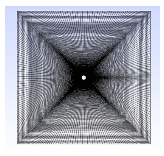
Figure 13.
Structured grid around a circular cylinder.
The flow Reynolds number based on cylinder diameter is Unlike the backward-facing step flow dominated by the step and the viscous wall, the flow physics in the case of a circular cylinder is dominated by vortex shedding and its subsequent breakdown downstream of the cylinder; accordingly, and because of the absence of walls, the value of is kept equal to 1.0 for all simulations. In order to compare to previous computational results, two values of were used, 0.5 and 0.7. A fine grid is used with and a coarser grid is used for Figure 14 shows the mean centerline streamwise velocity profile for . Our results agree with the PANS results of Girimaji et al. [16] both near the cylinder and far downstream and are in good agreement with the experimental data [26]. Figure 15 shows the mean centerline velocity profile for . Our results follow closely those of PANS across the whole domain and are in reasonable agreement with the experimental data.
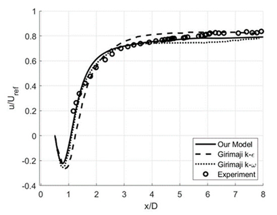
Figure 14.
The mean centerline streamwise velocity profile
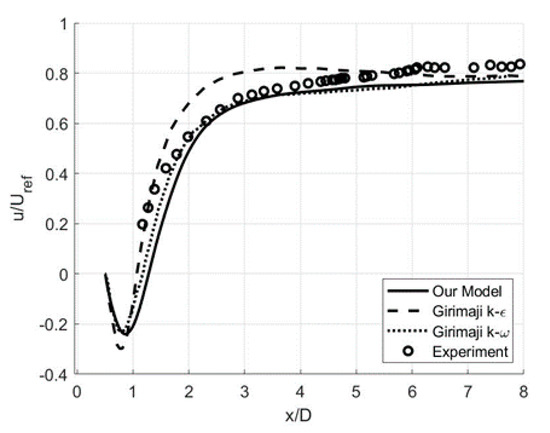
Figure 15.
The mean centerline streamwise velocity profile .
Figure 16 shows the vertical profile of the streamwise velocity at x/D = 1 and for Our model shows better agreement with the experimental data near the centerline and follows closely the PANS away from the centerline. When the grid is refined and is lowered to 0.5, the results from our model are significantly improved everywhere, as shown in Figure 17. Figure 18 shows the vertical profile of the streamwise velocity at x/D = 3 for . Though our model predictions are better than that of the PANS model, the predictions from the PANS are in better agreement with the experimental data. When the grid is refined and is lowered to 0.5, our model’s predictions are better everywhere than those of and PANS, as shown in Figure 19. Our model’s predictions are in excellent agreement with the experimental data across the entire profile.
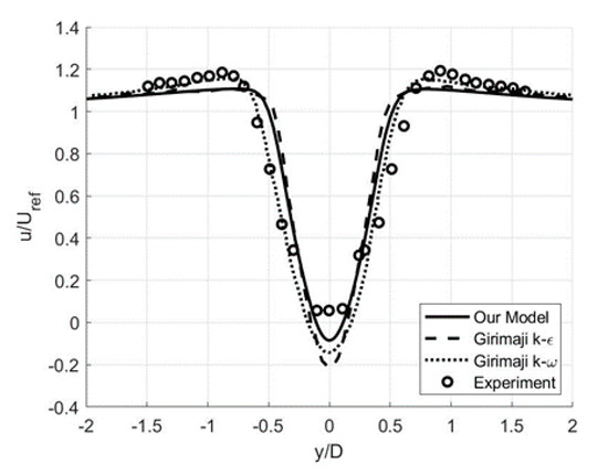
Figure 16.
The mean streamwise velocity profile at x/D = 1
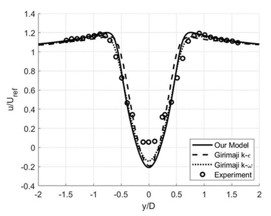
Figure 17.
The mean streamwise velocity profile at x/D = 1
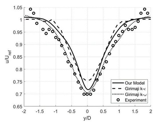
Figure 18.
The mean streamwise velocity profile at x/D = 3 .
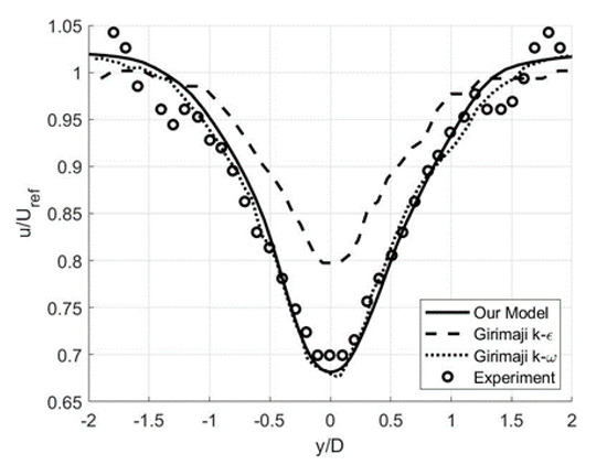
Figure 19.
The mean streamwise velocity profile at x/D = 3 .
The mean vertical velocity profile at x/D = 1 for is shown in Figure 20. Our results agree well with the experimental data and the results from the PANS. A refined grid and a lowering of to 0.5 resulted in improvements near the peak velocities and away from the centerline, Figure 21.
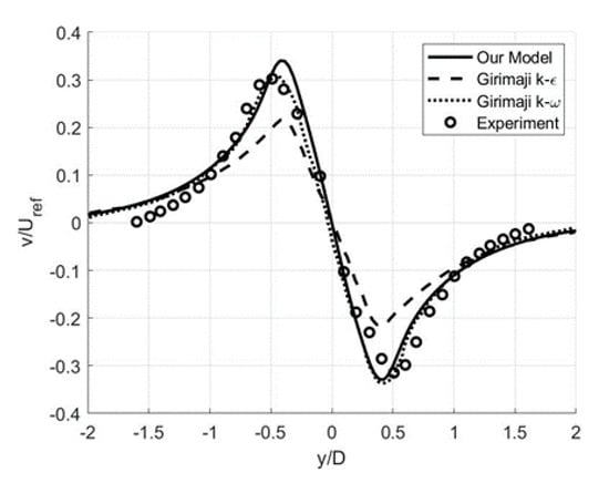
Figure 20.
The mean vertical velocity profile at x/D = 1 .
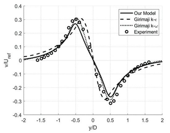
Figure 21.
The mean vertical velocity profile at x/D = 1 .
Figure 22 shows a Q-criterion iso-contours colored by velocity which illustrates the turbulent structures shed from the cylinder.
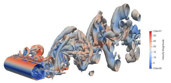
Figure 22.
Q-criterion iso-contours colored with velocity for Q = 500 .
4. Conclusions
A new Partially Averaged Navier-Stokes model has been derived. The model is based on the existing and PANS models. Menter’s [21] bridging approach is used. The new model is tested using two benchmark problems; the backward-facing step, representing wall-bounded flows, and flow over a circular cylinder, representing free shear flows. For comparison reasons, the PANS resolution control parameters were taken from the open literature with an appropriate grid resolution. For both benchmark problems, experimental data is used for comparison as well as existing computational results using PANS or .
For the backward-facing step problem, the mean velocity profile downstream of the step obtained by our model is found to be between that of the and models and in excellent agreement with the experimental data [25]. In addition, there was a marked improvement in the turbulent kinetic energy and Reynolds stress profiles predicted by our model.
For the circular cylinder, all mean velocity profiles predicted by our model; centerline streamwise, streamwise, and vertical; are in excellent agreement with the experimental data [26] for of 0.5. Our model agrees well with the PANS model and is everywhere better than the PANS model.
In conclusion, the PANS Bridging model proposed in this paper shows significant improvements in predictions over existing PANS models.
Author Contributions
Conceptualization, A.F.; methodology, A.F.; software, C.H.; validation, A.F., C.H.; formal analysis, A.F. and C.H.; investigation, C.H.; resources, C.H.; data curation, C.H.; writing—original draft preparation, A.F. and C.H.; writing—review and editing, A.F.; visualization, C.H.; supervision, A.F.; project administration, A.F.; funding acquisition, A.F. All authors have read and agreed to the published version of the manuscript.
Funding
This research received no external funding.
Acknowledgments
The computational resources used for this work were provided by the Alabama Supercomputer Authority. The second author was supported by a SMART scholarship from the US Army at Redstone Arsenal.
Conflicts of Interest
The authors declare no conflict of interest.
References
- Speziale, C.G. Turbulence Modeling for Time-Dependent RANS and VLES: A Review. AIAA J. 1998, 36, 173–184. [Google Scholar] [CrossRef]
- Le, H.; Moin, P.; Kim, J. Direct Numerical Simulation of Flow over a Backward Facing Step. J. Fluid Mech. 1997, 330, 349–374. [Google Scholar] [CrossRef]
- Kolmogorov, A.N. A Refinement of Previous Hypotheses Concerning the Local Structure of Turbulence in a Viscous Incompressible Fluid at High Reynolds Number. J. Fluid Mech. 1962, 13, 82–85. [Google Scholar] [CrossRef]
- Spalding, D.B. Kolmogorov’s two-equation model of turbulence. Proc. R. Socoety London Math. Phys. Eng. Sci. 1991, 434, 211–216. [Google Scholar] [CrossRef]
- Smagorinsky, J. General Circulation Experiments with the Primitive Equations. Mon. Weather. Rev. 1963, 93, 99–164. [Google Scholar] [CrossRef]
- Moin, P.; Kim, J. Numerical Investigation of Turbulent Channel Flow. J. Fluid Mech. 1982, 118, 341–377. [Google Scholar] [CrossRef]
- Germano, M.; Piomelli, U.; Moin, P.; Cabot, W.M. A Dynamic Subgrid-Scale Eddy Viscosity Model. Phys. Fluids A Fluid Dyn. 1991, 3, 1760–1765. [Google Scholar] [CrossRef]
- Germano, M. From RANS to DNS: Towards a Bridging Model. ERCOFTAC Series, 7. In Direct and Large-Eddy Simulation III; Voke, P.R., Sandham, N.D., Kleiser, L., Eds.; Kluwer Academic Publishers: Berlin, Germany, 1999; pp. 225–236. [Google Scholar]
- Spalart, P.R.; Jou, W.-H.; Strelets, M.; Allmaras, S.R. Comments on the Feasibility of LES for Wings, and on a Hybrid RANS/LES Approach. In Advances in DNS/LES, 1st AFOSR Int. Conf. On DNS/LES, Aug. 4–8, 1997; Greyden Press: Columbus, OH, USA, 1997. [Google Scholar]
- Squires, K.D.; Frosythe, J.R.; Spalart, P.R. Detached-Eddy Simulation of the Separated Flow Around a Forebody Cross-section. In ERCOFTAC Series, 16 “Direct and Large-Eddy Simulation IV”; Geurts, B.J., Friedrich, R., Metais, O., Eds.; Kluwer Academic Press: Berlin, Germany, 2001; Volume 8, pp. 481–500. [Google Scholar]
- Deck, S. Zonal-Detached-Eddy Simulation of the flow around a high-lift configuration. AIAA J. 2005, 43, 2372–2384. [Google Scholar] [CrossRef]
- Spalart, P.R.; Deck, S.; Shur, M.L.; Squires, K.D.; Strelets, M.K.; Travin, A.K. A new version of Detached-Eddy Simulation, resistant to ambiguous grid densities. Theor. Comp. Fluid Dyn. 2006, 20, 181–195. [Google Scholar] [CrossRef]
- Shur, M.L.; Spalart, P.R.; Strelets, M.K.; Travin, A. A hybrid RANS-LES model with delayed DES and wall-modeled LES capabilities. Int. J. Heat Fluid Flow 2008, 29, 1638–1649. [Google Scholar] [CrossRef]
- Girimaji, S. Partially Averaged Navier-Stokes Model for Turbulence: A Reynolds Averaged Navier-Stokes to Direct Numerical Simulation Bridging Method. J. Appl. Mech. 2006, 73, 413–421. [Google Scholar] [CrossRef]
- Frendi, A.; Tosh, A.; Girimaji, S. Flow Past a Backward Facing Step: Comparison of PANS, DES, and URANS Results with Experiments. Int. J. Comput. Methods Eng. Sci. Mech. 2006, 8, 23–38. [Google Scholar] [CrossRef]
- Girimaji, S.; Lakshmipathy, S. Partially Averaged Navier-Stokes Method for Turbulent Flows: K-ω Model Implementation. In Proceedings of the 44th AIAA Aerospace Sciences Meeting and Exhibit, Reno, NV, USA, 9–12 January 2006. [Google Scholar]
- Jones, W.; Launder, B. The Prediction of Laminarization with a Two-Equation Model of Turbulence. Int. J. Heat Mass Transf. 1972, 15, 301–314. [Google Scholar] [CrossRef]
- Wilcox, D.C. Reassessment of the Scale-Determining Equation for Advanced Turbulence Models. AIAA J. 1988, 26, 1299–1310. [Google Scholar] [CrossRef]
- Batten, P.; Goldberg, U.; Chakravarthy, S. LNS-An Approach Towards Embedded LES. In Proceedings of the 40th AIAA Aerospace Sciences Meeting & Exhibit, Reno, NV, USA, 14–17 January 2002. [Google Scholar]
- Speziale, C.G. Computing non-Equilibrium Flows with Time-Dependent RANS and VLES. In Proceedings of the 15th ICNMFD, Monterey, CA, USA, 24–28 June 1996. [Google Scholar]
- Menter, F.R. Two-Equation Eddy-Viscosity Turbulence Models for Engineering Applications. AIAA J. 1994, 32, 1598–1605. [Google Scholar] [CrossRef]
- OpenFOAM: The OpenFOAM Foundation. Available online: https://openfoam.org (accessed on 29 July 2020).
- Gmesh: A Three-Dimensional Finite Element Mesh Generator with Built-in Pre- and Post-Processing Facilities. Available online: https://gmsh.info/ (accessed on 29 July 2020).
- Harrison, C. Partially Averaged Navier-Stokes: A Bridging Model. Master’s Thesis, The University of Alabama in Huntsville, Huntsville, AL, USA, 2020. [Google Scholar]
- Driver, D.; Seegmiller, H. Features of a Reattaching Turbulent Shear Layer in Divergent Channel Flow. AIAA J. 1985, 23, 163–171. [Google Scholar] [CrossRef]
- Cantwell, B.; Coles, D. An Experimental Study of Entrainment and Transport in the Turbulent Near Wake of a Circular Cylinder. J. Fluid Mech. 1983, 136, 321–374. [Google Scholar] [CrossRef]
© 2020 by the authors. Licensee MDPI, Basel, Switzerland. This article is an open access article distributed under the terms and conditions of the Creative Commons Attribution (CC BY) license (http://creativecommons.org/licenses/by/4.0/).