The Effects of Grid Accuracy on Flow Simulations: A Numerical Assessment

Abstract

High-quality, accurate grid generation is a critical challenge in the computational simulation of fluid flows around complex geometries. In particular, the accuracy of the grids is an effective factor in order to achieve a successful numerical simulation. In the current study, we present a series of systematic numerical simulations for fluid flows around a NACA 0012 airfoil using different computational grid generation techniques, including the standard second-order, fourth-order compact, and Theodorsen transformation approaches, to assess the effects of grid accuracy on the flow solutions. The flow solvers are based on the second- and fourth-order schemes for spatial discretizations and Beam-Warming linearization method for time advancement. The obtained grids, as well as the metrics and the corresponding numerical flow solution for each grid generation technique, are compared and studied in detail. It is demonstrated that the quality and orthogonality of the grids is improved by using the fourth-order compact scheme. Moreover, the numerical assessment showed that the accuracy and the quality of the grids directly influence the numerical flow solutions. Finally, the higher-order accurate flow solvers are found to be more sensitive to the accuracy of the generated grid.

1. Introduction

One of the most critical subjects in computational fluid dynamics (CFD) simulation and modeling of flows around complex geometries is to generate high-quality grids on the flow region. The quality of the generated grid can strongly affect the accuracy of the numerical solution of a partial differential equation system [1,2,3,4]. In the past few decades, it has been established that the generation of high-quality grids is imperative for effective computations, and that can be equally important as improving the accuracy of the flow solver. Here, the grid quality means that the grid should be as smooth and orthogonal as possible in order to reduce the truncation error and carry out successful computational processes.

The structured and unstructured mesh generation techniques have been widely applied to a variety of flow solvers. Grid generation requires computational mapping from physical to computational space and geometry modeling. One of the most popular approaches for generating structured grids is solving a set of partial differential equations. The commonly used methods are elliptic and hyperbolic systems. Elliptic systems apply an appropriate control function to achieve grid smoothness and orthogonality. Another common method is conformal mapping containing an orthogonal transformation that yields nearly orthogonal grids in the physical space [5].

In addition to high-quality grids, it is necessary to employ high-order computational techniques to achieve high-accurate flow solutions. High-order accurate methods have been widely used for the solution of practical problems in fluid mechanics [6,7,8,9,10,11]. In Direct Numerical Simulation (DNS) and Large-Eddy Simulation (LES) of turbulent fluid flows and computational aeroacoustics, applying compact schemes is prevalent because of their spectral-like resolution, short size stencil, low dispersion and diffusion errors, and high-order accuracy [12,13,14,15,16,17,18]. It is, therefore, essential to carefully investigate the accuracy of these solutions.

Developing high-order unstructured mesh techniques is of particular interest, especially in the automatic mesh generation for commercial software. Furthermore, it is essential to develop high-order unstructured grids for high-order CFD solvers. Karman et al. [19] developed a three-dimensional mesh curving method based on an optimized mesh smoothing scheme, where they generated high-quality high-order meshes by transforming the smoothed nodes to the high-order meshes. Engvall and Evans [20] also investigated the generation of exact unstructured meshes from a geometrical point of view and proposed a surface reconstruction methodology to recover the exact computer-aided design geometries. Using the classical Winslow equations, Fortunato and Persson [21] introduced a new methodology for producing high-order unstructured curved meshes. In comparison with the optimization and elasticity analogies-based techniques, their methodology reduced the computational cost while preserving the accuracy of the curved elements. Additionally, Zhao et al. [22] developed a grid generation approach based on an improved radius basic function technique in order to generate a high-order curvilinear mesh. The proposed methodology was demonstrated to improve the accuracy of numerical solutions of curve-boundary problems.

The computational simulations of fluid mechanics problems are largely influenced by the accuracy and quality of the generated grids. Indeed, there exists an important link between the solution accuracy, mesh size, and mesh type [23]. Wang et al. [24] derived a fourth-order compact finite-difference scheme, which allowed unequal mesh-sizes to be used in all three dimensions for solving the Poisson’s equation. Their results verified that the proposed method delivered formal fourth-order accuracy of numerical solutions. In another study, Shirayama [25] evaluated the effects of grid quality on the accuracy and convergence of flow solutions and improved the grid quality by applying an adaptive gridding technique based on weight functions and model equations. To achieve high-quality Cartesian grids, a new simplified ghost-point approach was introduced by Farooq and Müller [26] for embedded solid boundaries. They specifically improved the accuracy of the Cartesian grids for compressible Euler equations to simulate transonic flow over a circular bump. In a recent study, Karcz and Kacperski [27] further concluded that the numerical results of fluid flow in the agitated vessel depend significantly on the grid density and geometrical mesh quality.

The grid orthogonality and smoothness are key factors in high-quality grid generation techniques. A number of studies in the literature have investigated the impacts of orthogonality of the grids on the predicted results and solution accuracy for a wide range of diverse CFD applications (e.g., [28,29,30,31,32,33,34]). Matsuno [2] developed a new orthogonal hyperbolic grid technique based on a high-order upwind approach and showed that the orthogonality and robustness of the generated grids result in highly accurate flow solutions. Moreover, it was concluded that low-order accurate methods are too dissipative to achieve orthogonal grids. Sankaranarayanan and Spaulding [28] also investigated the effects of the grid orthogonality and resolution on the solution accuracy of shallow water equations. The error analysis showed that the truncation error of first- and second-order derivative terms are reduced for orthogonal grids. Besides, it was shown by Bagade et al. [29] that the performance and accuracy of transient flow simulations strongly depend on the orthogonality of the grid. Bagade et al. [29] further performed a grid sensitivity analysis to demonstrate that the grid characteristics and properties are effective parameters in high accuracy flow computations. Finally, in a comprehensive computational study, Akcelik et al. [30] investigated the effects of boundary type, grid quality control function, and grid properties on their proposed orthogonal grid generation methodology. This grid generation technique was shown to provide an acceptable balance between controlling the grid orthogonality and aspect ratio.

It is well established that a numerical solution of fluid flow strongly depends on the quality of the generated grid. Yet, there exist no reliable criteria for measuring grid quality and its effects on the flow solution accuracy. For the structured grids, the transformation metrics and the corresponding Jacobian appear in the transformed governing equations in computational space. In the present work, therefore, we aim to systematically investigate the effects of grid accuracy on the numerical solution of flow problems with complex geometries. In that regard, a high-order compact finite-difference scheme is employed to assess the accuracy and quality of the grid. To this end, the accuracy of the geometric metrics of the grid produced by the second-order method is first compared with those obtained by the fourth-order compact method. The orthogonal grids produced by Theodorsen transformation are then compared with those generated through the second- and fourth-order schemes. Finally, to assess the effects of grid accuracy on flow solutions, the numerical simulation of compressible flows around NACA 0012 with different grid generation techniques are implemented and investigated in detail. The rest of this paper is organized as follows. In Section 2, the governing equations for compressible flows are derived. The numerical technique, including spacial discretization, temporal advancement, and spatial filtering, is then explained in Section 3. Section 4 provides the results of the high-order flow solver for several test cases. The elliptic grid generation and conformal mapping procedures are explained in Section 5 and Section 6, respectively. Section 7 compares the different grid generation techniques. Finally, the effect of grid accuracy on the flow solutions is studied in Section 8.

2. Governing Equations

The Navier-Stokes equations for compressible flows can be expressed in a general curvilinear frame of reference by

$$\frac{\partial \mathbf{Q}}{\partial t}+\frac{\partial \mathbf{F}}{\partial \xi }+\frac{\partial \mathbf{G}}{\partial \eta }+\frac{\partial \mathbf{H}}{\partial \zeta }=\frac{1}{Re}\left(\frac{\partial {\mathbf{F}}_{\upsilon }}{\partial \upsilon }+\frac{\partial {\mathbf{G}}_{\upsilon }}{\partial \eta }+\frac{\partial {\mathbf{H}}_{\upsilon }}{\partial \zeta }\right),$$

(1)

where t is the time, and $\xi$, $\eta$, and $\zeta$ are coordinate axes in the streamwise, spanwise, and vertical directions, respectively. Moreover, in the above equation, $\mathbf{Q}$ represents the conserved variable vector, $\mathbf{F}$, $\mathbf{G}$, and $\mathbf{H}$ denote the convective flux vectors, ${\mathbf{F}}_{\upsilon }$, ${\mathbf{G}}_{\upsilon }$, and ${\mathbf{H}}_{\upsilon }$ imply the viscous flux terms, and $Re$ is the reference Reynolds number. The vector of conserved variables is defined as

$$\mathbf{Q}=\frac{1}{J}{\left[\rho ,\rho u,\rho v,\rho w,E\right]}^{\mathrm{T}},$$

(2)

and the vectors of convective fluxes are defined as

$$\begin{array}{cc}\hfill \mathbf{F}& =\frac{1}{J}{\left[\rho U,\rho uU+{\xi }_{x}p,\rho vU+{\xi }_{y}p,\rho wU+{\xi }_{z}p,\left(E+p\right)U\right]}^{\mathrm{T}},\hfill \\ \hfill \mathbf{G}& =\frac{1}{J}{\left[\rho V,\rho uV+{\eta }_{x}p,\rho vV+{\eta }_{y}p,\rho wV+{\eta }_{z}p,\left(E+p\right)V\right]}^{\mathrm{T}},\hfill \\ \hfill \mathbf{H}& =\frac{1}{J}{\left[\rho W,\rho uW+{\zeta }_{x}p,\rho vW+{\zeta }_{y}p,\rho wW+{\zeta }_{z}p,\left(E+p\right)W\right]}^{\mathrm{T}}.\hfill \end{array}$$

(3)

Here, the superscript $\mathrm{T}$ indicates the transpose of the vector and

$$\left[\begin{array}{c}U\\ V\\ W\end{array}\right]=\left[\begin{array}{ccc}{\xi }_x& {\xi }_y& {\xi }_z\\ {\eta }_x& {\eta }_y& {\eta }_z\\ {\zeta }_x& {\zeta }_y& {\zeta }_z\end{array}\right]\left[\begin{array}{c}u\\ v\\ w\end{array}\right].$$

Also, u, v, and w are the Cartesian velocity components in x, y, and z directions, $\rho$ is the density, p is the pressure, E is the total energy, and

$$J=\frac{\partial \left(\xi ,\eta ,\zeta \right)}{\partial \left(x,y,z\right)}=\left|\begin{array}{ccc}{\xi }_x& {\xi }_y& {\xi }_z\\ {\eta }_x& {\eta }_y& {\eta }_z\\ {\zeta }_x& {\zeta }_y& {\zeta }_z\end{array}\right|$$

(4)

is the Jacobian of the transformation. The viscous flux terms in Equation (1) can be also expressed by

$$\begin{array}{cc}\hfill {\mathbf{F}}_{\upsilon }& =\frac{1}{J}{\left[0,{\xi }_x{\tau }_{xx}+{\xi }_y{\tau }_{xy}+{\xi }_z{\tau }_{xz},{\xi }_x{\tau }_{yx}+{\xi }_y{\tau }_{yy}+{\xi }_z{\tau }_{yz},{\xi }_x{\tau }_{zx}+{\xi }_y{\tau }_{zy}+{\xi }_z{\tau }_{zz},f^{*}\right]}^{\mathrm{T}},\hfill \\ \hfill {\mathbf{G}}_{\upsilon }& =\frac{1}{J}{\left[0,{\eta }_x{\tau }_{xx}+{\eta }_y{\tau }_{xy}+{\eta }_z{\tau }_{xz},{\eta }_x{\tau }_{yx}+{\eta }_y{\tau }_{yy}+{\eta }_z{\tau }_{yz},{\eta }_x{\tau }_{zx}+{\eta }_y{\tau }_{zy}+{\eta }_z{\tau }_{zz},g^{*}\right]}^{\mathrm{T}},\hfill \\ \hfill {\mathbf{H}}_{\upsilon }& =\frac{1}{J}{\left[0,{\zeta }_x{\tau }_{xx}+{\zeta }_y{\tau }_{xy}+{\zeta }_z{\tau }_{xz},{\zeta }_x{\tau }_{yx}+{\zeta }_y{\tau }_{yy}+{\zeta }_z{\tau }_{yz},{\zeta }_x{\tau }_{zx}+{\zeta }_y{\tau }_{zy}+{\zeta }_z{\tau }_{zz},h^{*}\right]}^{\mathrm{T}},\hfill \end{array}$$

(5)

in which $\tau$ indicates the viscous stress tensor. The components of the viscous stress tensor along with the expanded forms of $f^{*}$, $g^{*}$, and $h^{*}$ are presented in Appendix A. The system of equations represented in (1) is closed with the ideal-gas law and the assumption of a constant Prandtl number (see Appendix A). Finally, all variables appeared in Equations (1)–(5) are scaled by appropriate reference values; the cartesian and curvilinear coordinates by the characteristic length L, velocity components by the freestream velocity $u_{\infty }$, density and viscosity by the freestream density and viscosity, pressure by ${\rho }_{\infty }{u}_{\infty }^2$, and time by $L/u_{\infty }$. This normalization is leading to the definition of the reference Reynolds number $Re={\rho }_{\infty }{u}_{\infty }L/{\mu }_{\infty }$.

3. Numerical Method

3.1. Compact Finite Difference Scheme

The high-order compact scheme proposed by Lele [12] is applied to discretize the spatial derivatives in the dynamical governing equations. Here, using the fourth-order compact finite-difference method, the derivative $f^{\prime }$ of any scalar quantity f, including a transformation metric, a flux component, and a flow variable, can be obtained by

$$f_{i+1}^{\prime }+4f_i^{\prime }+f_{i-1}^{\prime }=\frac{3}{h}\left(f_{i+1}-f_{i-1}\right)+O\left(h^4\right),$$

(6)

in which the subscript i denotes the corresponding quantity at node i and h refers to the grid spacing difference.

For points close to the boundaries, we also considered high-order forward and backward compact schemes to preserve the tridiagonal form of the equations. The following formulations, therefore, were used to treat the physical boundary points at nodes $i=1$ and $i=I_N$, respectively:

$$f_1^{\prime }+3f_2^{\prime }=\frac{1}{6h}(-17f_1+9f_2+9f_3-f_4)+O\left(h^4\right),$$

(7)

$$3f_{I_N-1}^{\prime }+f_{I_N}^{\prime }=\frac{1}{6h}(17f_{I_N}-9f_{I_N-1}-9f_{I_N-2}+f_{I_N-3})+O\left(h^4\right).$$

(8)

This fourth-order accurate scheme near the boundaries allowed us to retain the accuracy of the numerical solution over the entire computational domain.

3.2. Temporal Discretization

The implicit linearization method for the finite-difference scheme proposed by Beam and Warming [35] is applied for the time advancement. The implicit algorithm is further extended to three dimensions. Using Equation (1) and the trapezoidal formula (see [35]), we can express the time-marching equation as

$$\begin{array}{cc}\hfill {\mathbf{Q}}^{n+1}={\mathbf{Q}}^n-\frac{\Delta t}{2}& \left[{\left(\frac{\partial }{\partial \xi }\left(\mathbf{F}-\frac{1}{Re}{\mathbf{F}}_{\upsilon }\right)+\frac{\partial }{\partial \eta }\left(\mathbf{G}-\frac{1}{Re}{\mathbf{G}}_{\upsilon }\right)+\frac{\partial }{\partial \zeta }\left(\mathbf{H}-\frac{1}{Re}{\mathbf{H}}_{\upsilon }\right)\right)}^n\right.\hfill \\ \hfill & +\left.{\left(\frac{\partial }{\partial \xi }\left(\mathbf{F}-\frac{1}{Re}{\mathbf{F}}_{\upsilon }\right)+\frac{\partial }{\partial \eta }\left(\mathbf{G}-\frac{1}{Re}{\mathbf{G}}_{\upsilon }\right)+\frac{\partial }{\partial \zeta }\left(\mathbf{H}-\frac{1}{Re}{\mathbf{H}}_{\upsilon }\right)\right)}^{n+1}\right]\hfill \\ \hfill & +O\left({\Delta t}^3\right),\hfill \end{array}$$

(9)

in which ${\mathbf{Q}}^{n+1}$ is the updated value of ${\mathbf{Q}}^n$ at the iteration $n+1$, and $\Delta t$ is the time step size. A local Taylor expansion about ${\mathbf{Q}}^n$ results in a linear relationship between the convective flux vector ${\mathbf{F}}^{n+1}$ and the conserved variable vector ${\mathbf{Q}}^{n+1}$ in a way that,

$${\mathbf{F}}^{n+1}={\mathbf{F}}^n+{\mathbf{A}}^n\left({\mathbf{Q}}^{n+1}-{\mathbf{Q}}^n\right)+\mathrm{O}\left({\Delta t}^2\right),$$

(10)

where $\mathbf{A}$ is the Jacobian matrix and ${\mathbf{A}}^n=\partial {\mathbf{F}}^n/\partial {\mathbf{Q}}^n$. Moreover, the Alternating-Direction-Implicit (ADI) method [36] and the fractional step algorithm [37] were next applied to Equation (9) to take advantage of efficient multi-dimensional implicit algorithms. By applying similar linearization to other flux terms, Equation (9) can be reduced to

$$\begin{array}{cc}\hfill \left[\mathbf{I}+\frac{\Delta t}{2}\frac{\partial }{\partial \xi }\left({\mathbf{A}}^n-\frac{1}{Re}{\mathbf{A}}_{\upsilon }^n\right)\right]& \left[\mathbf{I}+\frac{\Delta t}{2}\frac{\partial }{\partial \eta }\left({\mathbf{B}}^n-\frac{1}{Re}{\mathbf{B}}_{\upsilon }^n\right)\right]\hfill \\ \hfill & \left[\mathbf{I}+\frac{\Delta t}{2}\frac{\partial }{\partial \zeta }\left({\mathbf{C}}^n-\frac{1}{Re}{\mathbf{C}}_{\upsilon }^n\right)\right]{\mathbf{Q}}^{n+1}\hfill \\ \hfill =& \left[\mathbf{I}+\frac{\Delta t}{2}\frac{\partial }{\partial \xi }\left({\mathbf{A}}^n-\frac{1}{Re}{\mathbf{A}}_{\upsilon }^n\right)\right]\left[\mathbf{I}+\frac{\Delta t}{2}\frac{\partial }{\partial \eta }\left({\mathbf{B}}^n-\frac{1}{Re}{\mathbf{B}}_{\upsilon }^n\right)\right]\hfill \\ \hfill & \left[\mathbf{I}+\frac{\Delta t}{2}\frac{\partial }{\partial \zeta }\left({\mathbf{C}}^n-\frac{1}{Re}{\mathbf{C}}_{\upsilon }^n\right)\right]{\mathbf{Q}}^n\hfill \\ \hfill -\Delta t\left[\frac{\partial }{\partial \xi }\left({\mathbf{F}}^n-\frac{1}{Re}{\mathbf{F}}_{\upsilon }^n\right)\right.& +\left.\frac{\partial }{\partial \eta }\left({\mathbf{G}}^n-\frac{1}{Re}{\mathbf{G}}_{\upsilon }^n\right)+\frac{\partial }{\partial \zeta }\left({\mathbf{H}}^n-\frac{1}{Re}{\mathbf{H}}_{\upsilon }^n\right)\right],\hfill \end{array}$$

(11)

where $\mathbf{I}$ is the identity matrix, and ${\mathbf{B}}^n=\partial {\mathbf{G}}^n/\partial {\mathbf{Q}}^n$ and ${\mathbf{C}}^n=\partial {\mathbf{H}}^n/\partial {\mathbf{Q}}^n$ are Jacobian matrices. Similarly,

$${\mathbf{A}}_{\upsilon }^n=\frac{\partial {\mathbf{F}}_{\upsilon }^n}{\partial {\mathbf{Q}}^n},{\mathbf{B}}_{\upsilon }^n=\frac{\partial {\mathbf{G}}_{\upsilon }^n}{\partial {\mathbf{Q}}^n},{\mathbf{C}}_{\upsilon }^n=\frac{\partial {\mathbf{H}}_{\upsilon }^n}{\partial {\mathbf{Q}}^n}.$$

(12)

Using the procedure explained above, we were able to reduce the complexity of the problem from an immense matrix inversion (see Equation (9)) to a series of tridiagonal matrix inversion problems for which efficient solution algorithms exist. To solve Equation (11), three one-dimensional sweeps are employed,

$$\left[\mathbf{I}+\frac{\Delta t}{2}\frac{\partial }{\partial \xi }\left({\mathbf{A}}^n-\frac{1}{Re}{\mathbf{A}}_{\upsilon }^n\right)\right]\Delta {\mathbf{Q}}^{**}=\mathrm{RHS},$$

(13a)

$$\left[\mathbf{I}+\frac{\Delta t}{2}\frac{\partial }{\partial \eta }\left({\mathbf{B}}^n-\frac{1}{Re}{\mathbf{B}}_{\upsilon }^n\right)\right]\Delta {\mathbf{Q}}^{*}=\Delta {\mathbf{Q}}^{**},$$

(13b)

$$\left[\mathbf{I}+\frac{\Delta t}{2}\frac{\partial }{\partial \zeta }\left({\mathbf{C}}^n-\frac{1}{Re}{\mathbf{C}}_{\upsilon }^n\right)\right]\Delta {\mathbf{Q}}^n=\Delta {\mathbf{Q}}^{*},$$

(13c)

in which $\Delta {\mathbf{Q}}^{**}$ and $\Delta {\mathbf{Q}}^{*}$ are mediator variables, $\Delta {\mathbf{Q}}^n={\mathbf{Q}}^{n+1}-{\mathbf{Q}}^n$, and $\mathrm{RHS}$ refers the right-hand side of Equation (11). Equation (13a)–(13c) are sweeps in the $\xi$, $\eta$, and $\zeta$ directions, respectively. By substituting Equation (6) with first-order derivatives into Equation (13a)–(13c), we obtain the following system of equations:

$$\begin{array}{cc}\hfill (-\frac{\Delta t}{2}\left({\mathbf{A}}_{i-1}-\frac{1}{Re}{\mathbf{A}}_{\upsilon ,\left(i-1\right)}\right)& +\frac{1}{6}){\Delta \mathbf{Q}}_{i-1}^{**}+\frac{2}{3}{\Delta \mathbf{Q}}_i^{**}\hfill \\ \hfill & +\left(\frac{\Delta t}{2}\left({\mathbf{A}}_{i+1}-\frac{1}{Re}{\mathbf{A}}_{\upsilon ,\left(i+1\right)}\right)+\frac{1}{6}\right){\Delta \mathbf{Q}}_{i+1}^{**}\hfill \\ \hfill & =\mathrm{RHS},\hfill \end{array}$$

(14a)

$$\begin{array}{cc}\hfill (-\frac{\Delta t}{2}\left({\mathbf{B}}_{j-1}-\frac{1}{Re}{\mathbf{B}}_{\upsilon ,\left(j-1\right)}\right)& +\frac{1}{6}){\Delta \mathbf{Q}}_{j-1}^{*}+\frac{2}{3}{\Delta \mathbf{Q}}_j^{*}\hfill \\ \hfill & +\left(\frac{\Delta t}{2}\left({\mathbf{B}}_{j+1}-\frac{1}{Re}{\mathbf{B}}_{\upsilon ,\left(j+1\right)}\right)+\frac{1}{6}\right){\Delta \mathbf{Q}}_{j+1}^{*}\hfill \\ \hfill & =\frac{1}{6}\left({\Delta \mathbf{Q}}_{j-1}^{**}+4{\Delta \mathbf{Q}}_j^{**}+{\Delta \mathbf{Q}}_{j+1}^{**}\right),\hfill \end{array}$$

(14b)

$$\begin{array}{cc}\hfill (-\frac{\Delta t}{2}\left({\mathbf{C}}_{k-1}-\frac{1}{Re}{\mathbf{C}}_{\upsilon ,\left(k-1\right)}\right)& +\frac{1}{6}){\Delta \mathbf{Q}}_{k-1}^n+\frac{2}{3}{\Delta \mathbf{Q}}_k^n\hfill \\ \hfill & +\left(\frac{\Delta t}{2}\left({\mathbf{C}}_{k+1}-\frac{1}{Re}{\mathbf{C}}_{\upsilon ,\left(k+1\right)}\right)+\frac{1}{6}\right){\Delta \mathbf{Q}}_{k+1}^n\hfill \\ \hfill & =\frac{1}{6}\left({\Delta \mathbf{Q}}_{k-1}^{*}+4{\Delta \mathbf{Q}}_k^{*}+{\Delta \mathbf{Q}}_{k+1}^{*}\right).\hfill \end{array}$$

(14c)

Here, the updated value of the variable vector ${\mathbf{Q}}^{n+1}$ is obtained through calculating $\Delta {\mathbf{Q}}^n={\mathbf{Q}}^{n+1}-{\mathbf{Q}}^n$ from Equation (14c). The above set of equations describes a system of tridiagonal matrix inversion problem solved by Thomas algorithm.

3.3. Spatial Filtering

The nonlinear convective terms in the Navier-Stokes equations are the major source of instabilities and irregularities. The numerical instabilities result in a continuous and unrestricted generation of high-frequency wave modes. Therefore, incorporating a high-order low-pass filter into the numerical methodology is essential to handle such instabilities. Here, we implemented a high-order non-dispersive compact spatial filtering technique [38,39] as part of the numerical approach. The implicit filter applied to the solution vector can be expressed as

$${\beta }_f{\widehat{\varphi }}_{i-1}+{\widehat{\varphi }}_i+{\beta }_f{\widehat{\varphi }}_{i+1}=\sum _{n=0}^N\frac{b_n}{2}\left({\varphi }_{i+n}+{\varphi }_{i-n}\right),$$

(15)

where ${\widehat{\varphi }}_i$ is the filtered function of ${\varphi }_i$ at grid point i, ${\beta }_f$ is the coefficient of implicit terms, $b_n$ is the coefficient of explicit terms for different orders of filter, and $2\times N$ is the order of the filter. For a sixth-order filter, we have,

$$b_0=\frac{11}{16}+\frac{5}{8}{\beta }_f,b_1=\frac{15}{32}+\frac{17}{16}{\beta }_f,b_2=-\frac{3}{16}+\frac{3}{8}{\beta }_f,b_3=-\frac{1}{32}-\frac{1}{16}{\beta }_f,$$

(16)

where ${\beta }_f=0.4$. The filtering is carried out on the conserved variable vector obtained from Equation (14) after each time step and estimated using Thomas algorithm, a typical tridiagonal matrix solver. Furthermore, the sixth-order forward and backward filtering technique was applied for near boundary points,

$$\begin{array}{c}\hfill {\beta }_f{\widehat{\varphi }}_{i-1}+{\widehat{\varphi }}_i+{\beta }_f{\widehat{\varphi }}_{i+1}=\sum _{n=1}^7{a}_{n,i}{\varphi }_n(i=2,3),\end{array}$$

(17a)

$$\begin{array}{c}\hfill {\beta }_f{\widehat{\varphi }}_{i-1}+{\widehat{\varphi }}_i+{\beta }_f{\widehat{\varphi }}_{i+1}=\sum _{n=0}^6{a}_{I_N-n,i}{\varphi }_{I_N-n}(i=I_N-2,I_N-1).\end{array}$$

(17b)

The coefficients of the right-hand side of the above equations, $a_n$, are derived using Taylor and Fourier-series analyses and can be found in, for example, Gaitonde and Visbal [40]. The values at the boundaries, nodes $i=1$ and $I_N$, are determined explicitly through prescribed boundary conditions. Thus, the tridiagonal structure of the filtering was maintained entirely.

4. Flow Solution Results

In this section, we first carry out a series of numerical simulations to verify and validate the current high-order compact flow solver against experimental results for fluid flow over a flat plate and a NACA 0012 airfoil. The accuracy of the numerical method and hence the flow solver is also assessed for the flow inside a Shubinn nozzle.

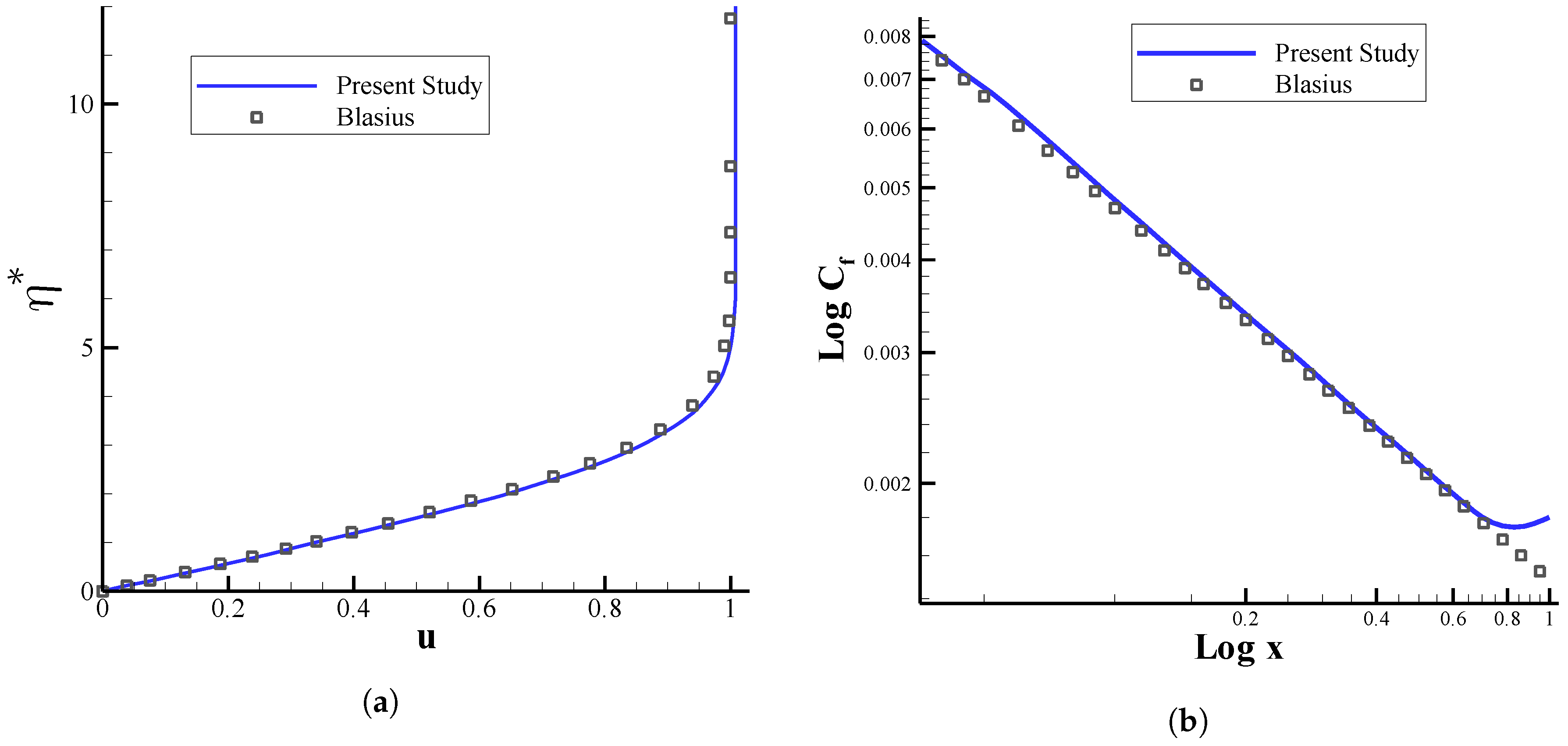
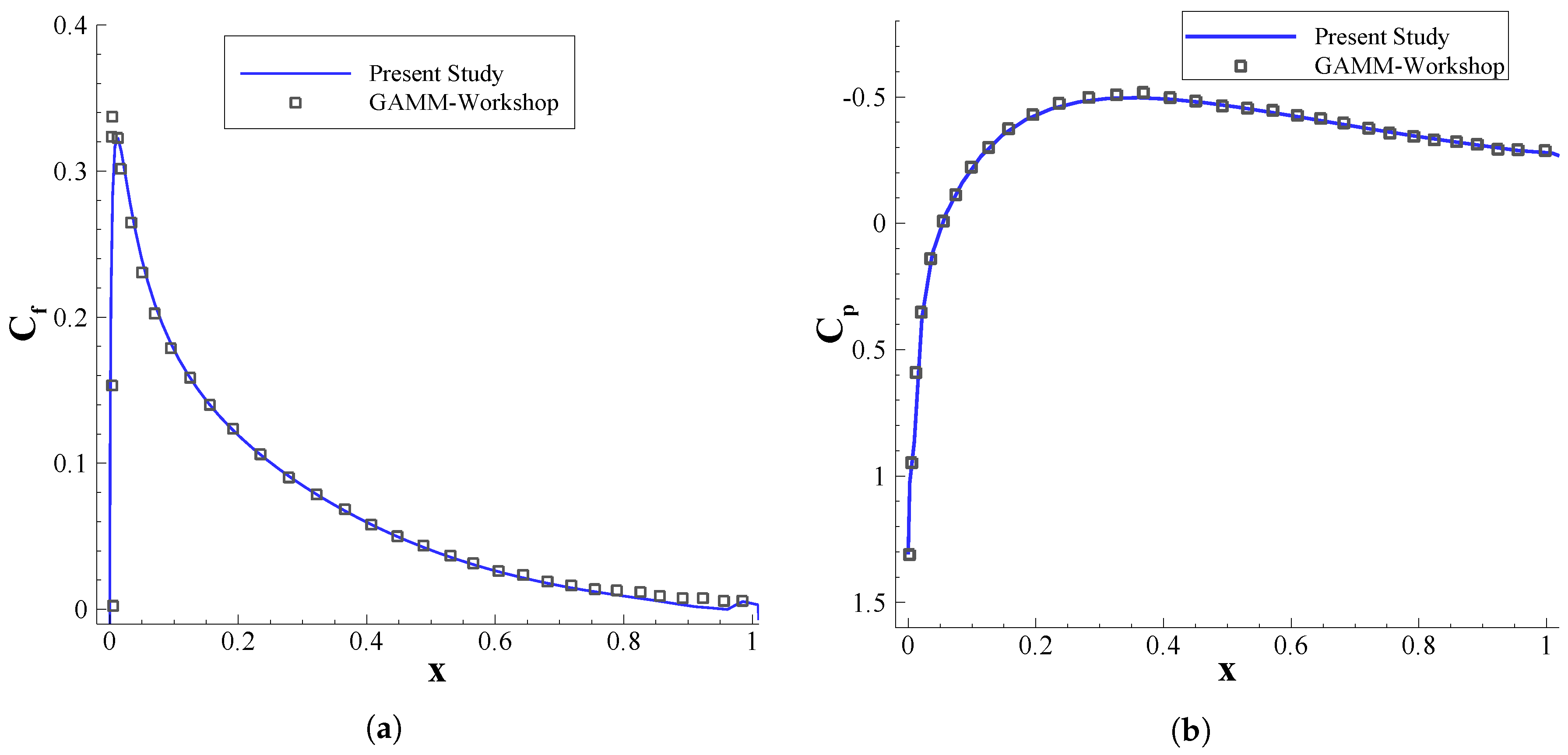
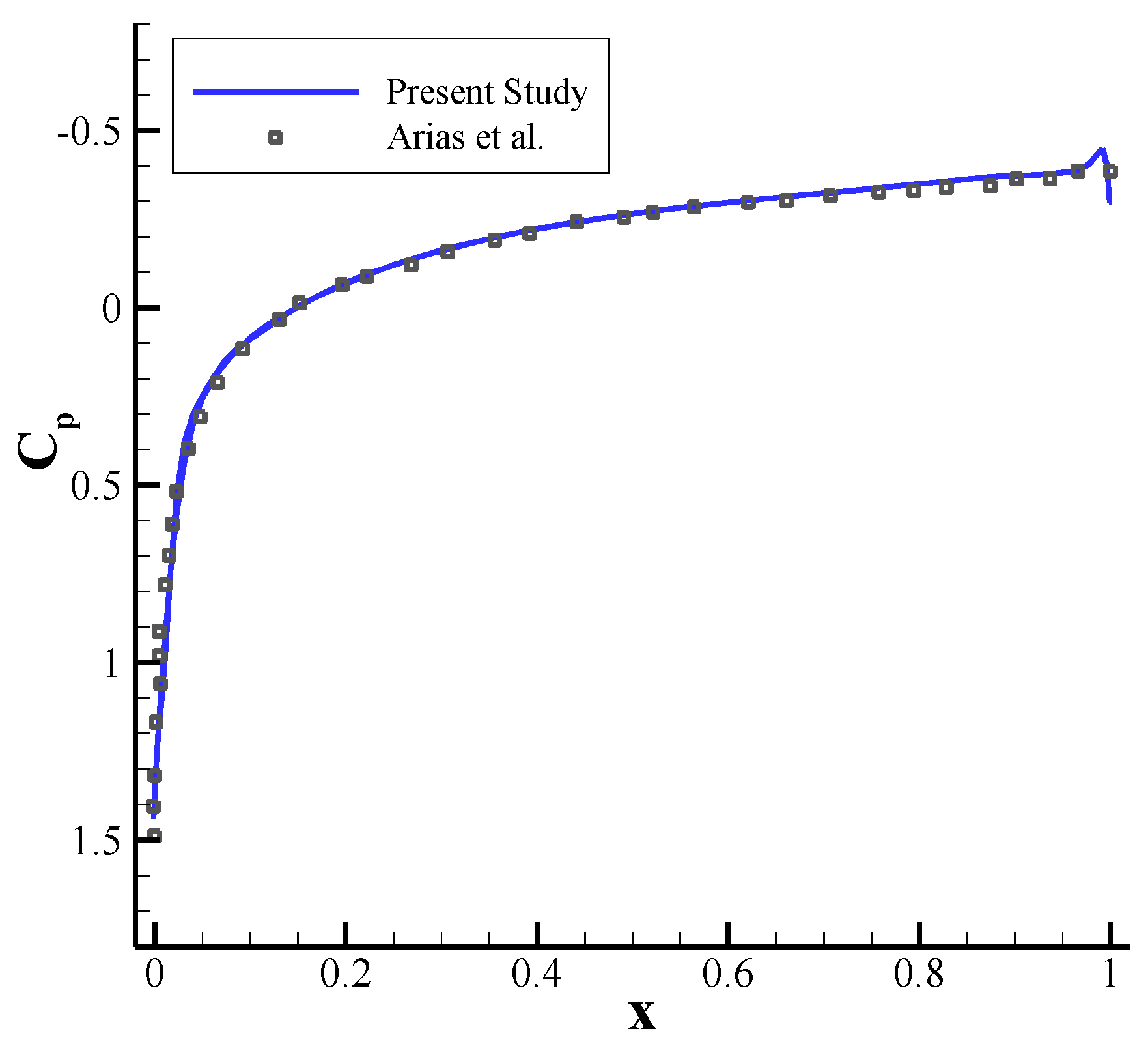
4.1. Numerical Validation

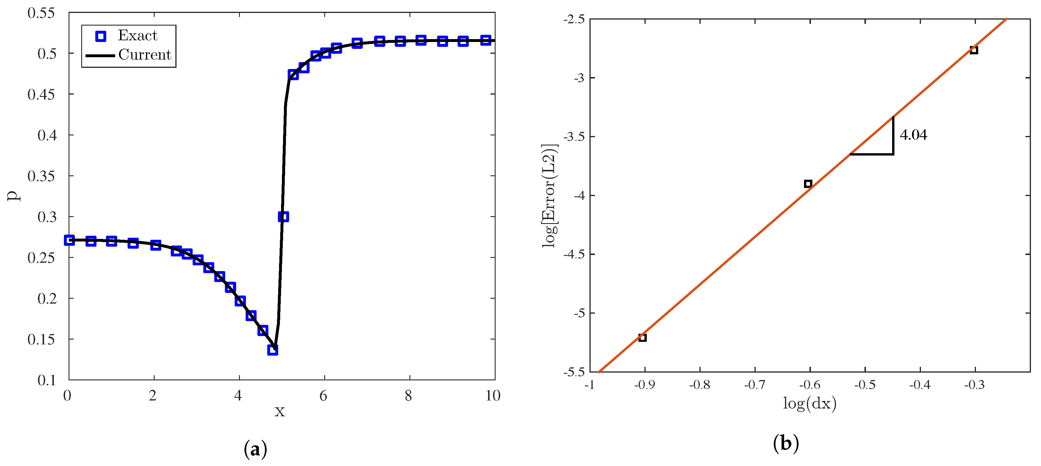
The two-dimensional laminar viscous flow over a flat plate with upstream conditions of $Ma=0.2$ and $Re=200\times {10}^3$ is solved using the high-order compact method. The profiles of horizontal velocity and friction coefficient are shown and compared with the classical Blasius solution for the flat-plate problem in Figure 1. The velocity profile is plotted against the non-dimensional position variable ${\eta }^{*}$; in the Blasius solution, ${\eta }^{*}=y\sqrt{u_{\infty }/\upsilon x}$ is a non-dimensional quantity that combines both x and y positions. The skin fiction coefficient, $C_f=2{\tau }_w/\rho u_{\infty }$ where ${\tau }_w$ is the wall shear stress, is also plotted along the length of the plate in Figure 1b. As it can be observed from Figure 1, there exist an excellent agreement between the current numerical solution and those obtained from the Blasius boundary layer solution for flow over a flat plate. The rise of the skin friction coefficient at the trailing edge of the flat plate is explained by the triple-deck theory that is not considered in the Blasius solution (see [41] for more details).

Further, we examined the fourth-order compact flow solver by simulating the flow field around a NACA 0012 airfoil with a Mach number of $0.85$ and a Reynolds number of 500. The profiles of the pressure and skin friction coefficients are presented in Figure 2. These profiles are well-matched with those of GAMM-Workshop [42]. Besides, we considered an inviscid supersonic flow around the NACA 0012 airfoil with $Ma=1.2$ to validate the correct behavior of the solver for supersonic inviscid flows as well. Figure 3 presents the pressure coefficient distribution over the airfoil, where the numerical results are compared with those obtained by Arias et al. [43]. Again, there is an excellent agreement between the two. It should be noted here that the grid around the NACA 0012 airfoil is generated using the elliptic method in x and y directions where $N_x=129$ and $N_y=37$. In the z direction the grid is uniform with $N_z=37$. In this study, the flow results of the NACA 0012 airfoil are presented in mid-plane in the z direction. The inflow and outflow boundary conditions are applied at the inlet and outlet, respectively. The wall boundary condition as well as adiabatic condition is used for the surface of the airfoil.

4.2. Accuracy Study

In order to assess the accuracy of the current compact finite-difference solver, we simulated the one-dimensional flow inside the Shubbin nozzle (see [44]) and compared the results with its corresponding exact solution. The cross-sectional area of a Shubbin nozzle is defined as

$$S\left(x\right)=1.398+0.347\left[tanh\left(0.8x-0.4\right)\right].$$

(18)

The inflow conditions are described as

$${\rho }_{in}=0.05008261,p_{in}=0.2712900,u_{in}=1.0991840,Ma=1.262214,$$

and for the outflow $p_{out}=0.5156000$. The pressure changes inside the Nozzle is demonstrated in Figure 4a. The analytical solution to the problem is also indicated in this figure, and it can be observed that the result of the present compact method agrees quite well with the exact solution.

Further, the $L2$-norm error is calculated to estimate the accuracy order of the solution. The $L2$-norm error can be defined as

$$E_{L2}=\sqrt{\frac{1}{N}\sum _{j=1}^N{(p^j-{p_e}^j)}^2},$$

(19)

where p and $p_e$ are the values of the pressure for the compact method solver and the exact solution, respectively. Figure 4b shows the $L2$-norm error, and it can be observed that the compact method presented in this study provides a fourth-order accurate solution.

5. Grid Generation

Elliptic Method

The elliptic grid generation method is based on solving a pair of Poisson equations in the computational domain with the desired grid points on the boundary of the physical domain, where the interior points can be determined by the solution of the following equations [45]:

$$\begin{array}{cc}\hfill & {\xi }_{xx}+{\xi }_{yy}=P(\xi ,\eta ),\hfill \\ \hfill & {\eta }_{xx}+{\eta }_{yy}=Q(\xi ,\eta ).\hfill \end{array}$$

(20)

Here, P and Q are the control functions. By interchanging the roles of dependent ($\xi ,\eta ,\zeta$) and independent variables ($x,y,z$), one can arrive at

$$\begin{array}{cc}\hfill & \alpha x_{\xi \xi }-2\beta x_{\xi \eta }+\gamma x_{\eta \eta }=-J^2(P{x}_{\xi }+Q{x}_{\eta }),\hfill \\ \hfill & \alpha y_{\xi \xi }-2\beta y_{\xi \eta }+\gamma y_{\eta \eta }=-J^2(P{y}_{\xi }+Q{y}_{\eta }),\hfill \end{array}$$

(21)

where

$$\begin{array}{cc}\hfill \alpha & =x_{\eta }^2+y_{\eta }^2,\hfill \\ \hfill \beta & =x_{\eta }{x}_{\xi }+y_{\eta }{y}_{\xi },\hfill \\ \hfill \gamma & =x_{\xi }^2+y_{\xi }^2,\hfill \end{array}$$

(22)

and J is the transformed Jacobian defined by $J=x_{\xi }{y}_{\eta }-x_{\eta }{y}_{\xi }$.

In order to control the grid attributes in the boundaries, grid spacing, and the orientation of coordinate lines, the control functions P and Q are defined as [46]

$$\begin{array}{cc}\hfill P& =P_L{e}^{-a_L(\eta -{\eta }_l)}+P_U{e}^{-a_U({\eta }_{max}-\eta )},\hfill \\ \hfill Q& =Q_L{e}^{-b_L(\eta -{\eta }_l)}+Q_U{e}^{-b_U({\eta }_{max}-\eta )},\hfill \end{array}$$

(23)

where $a_L$, $a_U$, $b_L$, and $b_U$ are positive constants that control the orthogonality and stretching grid nodes near the boundaries. Moreover, the functions $P_L$, $Q_L$, $P_U$, and $Q_U$ are defined near the lower and upper boundaries (see Sorenson [46] for more detail). Furthermore, to impose the orthogonality condition near the boundaries, the following equation is employed:

$$\nabla \xi ·\nabla \eta =|\nabla \xi |·|\nabla \eta |cos\theta .$$

(24)

After applying some simplifications, Equation (24) is reduced to

$$x_{\xi }{x}_{\eta }+y_{\xi }{y}_{\eta }=-{\left[(x_{\eta }^2+y_{\eta }^2)(x_{\xi }^2+y_{\xi }^2)\right]}^{\frac{1}{2}}cos\theta ,$$

(25)

where $x_{\eta }$ and $y_{\eta }$ can be expressed for $\theta =\pi /2$ as

$$\begin{array}{c}\hfill x_{\eta }=\frac{-s_{\eta }{y}_{\xi }}{{(x_{\xi }^2+y_{\xi }^2)}^{\frac{1}{2}}},\\ \hfill y_{\eta }=\frac{-s_{\eta }{x}_{\xi }}{{(x_{\xi }^2+y_{\xi }^2)}^{\frac{1}{2}}},\end{array}$$

(26)

in which

$$s_{\eta }={(x_{\eta }^2+y_{\eta }^2)}^{\frac{1}{2}}.$$

(27)

Furthermore, in order to avoid the numerical instability, especially when the control functions P and Q impose large values, the following upwind scheme is utilized for the first-order spatial derivatives:

$$\begin{array}{c}\hfill 5f_{i+1}^{\prime }+8f_i^{\prime }-f_{i-1}^{\prime }=\frac{12(f_{i+1}-f_i)}{h}+O\left(h^4\right)\mathrm{if}P\mathrm{or}Q>0,\\ \hfill -f_{i+1}^{\prime }-8f_i^{\prime }+5f_{i-1}^{\prime }=\frac{12(f_i-f_{i-1})}{h}+O\left(h^4\right)\mathrm{if}P\mathrm{or}Q<0.\end{array}$$

(28)

For the second-order derivatives, the fourth-order compact scheme is used [12],

$$f{″}_{i+1}+10f{″}_i+f{″}_{i-1}=12\frac{f_{i+1}-2f_i+f_{i-1}}{h^2}+O\left(h^4\right).$$

(29)

Equations (28) and (29) are also applied in the $\eta$ direction. As a result, there are five coupled equations at each point, namely,

$$\alpha x_{\xi \xi }-2\beta x_{\xi \eta }+\gamma x_{\eta \eta }=0,$$

(30a)

$$\begin{array}{c}\hfill 5x_{i+1}^{\prime }+8x_i^{\prime }-x_{i+1}^{\prime }=12\frac{(x_{i+1}-x_i)}{h}+O\left(h^4\right)\mathrm{if}P\mathrm{or}Q\ge 0,\\ \hfill -x_{i+1}^{\prime }-8x_i^{\prime }+5x_{i-1}^{\prime }=12\frac{(x_i-x_{i-1})}{h}+O\left(h^4\right)\mathrm{if}P\mathrm{or}Q<0,\end{array}$$

(30b)

$$\begin{array}{c}\hfill 5x_{j+1}^{\prime }+8x_j^{\prime }-x_{j+1}^{\prime }=12\frac{(x_{j+1}-x_j)}{h}+O\left(h^4\right)\mathrm{if}P\mathrm{or}Q\ge 0,\\ \hfill -x_{j+1}^{\prime }-8x_j^{\prime }+5x_{j-1}^{\prime }=12\frac{(x_j-x_{j-1})}{h}+O\left(h^4\right)\mathrm{if}P\mathrm{or}Q<0,\end{array}$$

(30c)

$$x{″}_{i+1}+10x{″}_i+x{″}_{i-1}=12\frac{x_{i+1}-2x_i+x_{i-1}}{h^2}+O\left(h^4\right),$$

(30d)

$$x{″}_{j+1}+10x{″}_j+x{″}_{j-1}=12\frac{x_{j+1}-2x_j+x_{j-1}}{h^2}+O\left(h^4\right),$$

(30e)

where subscripts i and j indicates the $\xi$- and $\eta$-direction, respectively. The above equations can be written in the following matrix form:

$$AX=B,$$

(31)

where

$$A=\left[\begin{array}{ccccc}0& J^{2}Q(\xi ,\eta )& \gamma & J^{2}P(\xi ,\eta )& \alpha \\ -12a_5& a2& 0& 0& 0\\ 24& 11& 10& 0& 0\\ -12a_5& 0& 0& a_2& 0\\ 24& 0& 0& 0& 10\end{array}\right],X=\left[\begin{array}{c}x\\ x_{\eta }\\ x_{\eta \eta }\\ x_{\xi }\\ x_{\xi \xi }\end{array}\right],$$

(32)

and

$$B=\left[\begin{array}{c}2\beta x_{\xi \eta }{|}_{(i,j)}\\ 12(a_4{x}_{i,j+1}+a_6{x}_{i,j-1})-a_1{x}_{\eta }{{|}_{(i,j-1)}-a_3{x}_{\eta }|}_{(i,j+1)}\\ 12(x_{i,j+1}+x_{i,j-1})-x_{\eta \eta }{{|}_{(i,j-1)}-x_{\eta \eta }|}_{(i,j+1)}\\ 12(a_4{x}_{i+1,j}+a_6{x}_{i-1,j})-a_1{x}_{\xi }{{|}_{(i-1,j)}-a_3{x}_{\xi }|}_{(i+1,j)}\\ 12(x_{i+1,j}+x_{i-1,j})-x_{\xi \xi }{{|}_{(i-1,j)}-x_{\xi \xi }|}_{(i+1,j)}\end{array}\right].$$

(33)

The coefficients $a_1$ to $a_6$ are reported in

Table 1. Values of constant coefficients of Equations (32) and (33).

If  P  or  $\mathit{Q}\ge 0$						If  P  or  $\mathit{Q}<0$
$a_1$	$a_2$	$a_3$	$a_4$	$a_5$	$a_6$	$a_1$	$a_2$	$a_3$	$a_4$	$a_5$	$a_6$
$-1$	8	5	1	$-1$	0	5	8	$-1$	0	1	$-1$

. The above system of equations is then solved using the Jacobi point iteration method. A similar approach is also applied in the y-direction. Again, it is worth mentioning here that the grid is uniform in the z-direction.

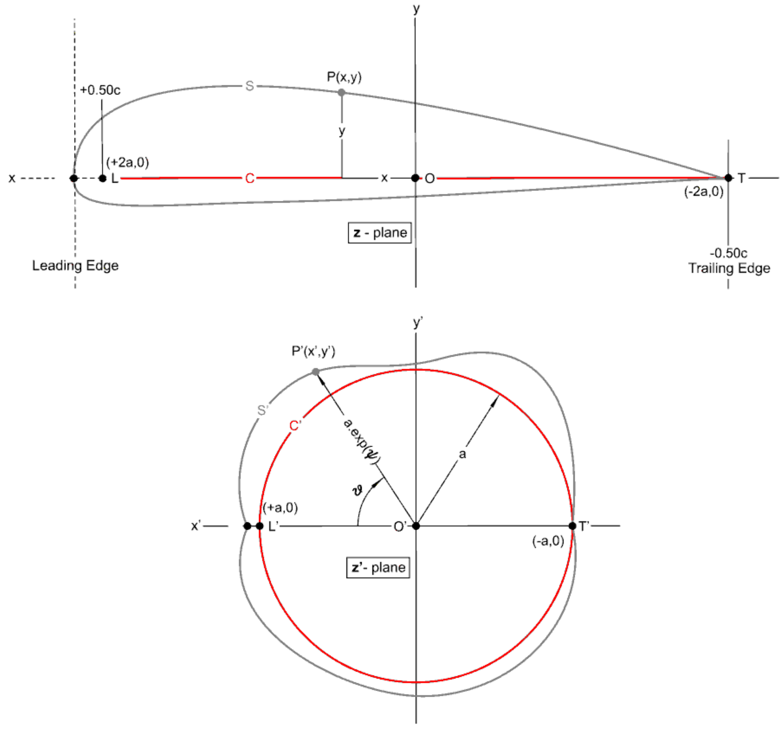
6. Conformal Mapping

In the calculation of flow around airfoils, it is often useful to map the exterior flow field of an airfoil conformally onto the interior of a circle. A direct, point-by-point transformation of an airfoil onto a circle can be performed in two distinct steps using the method suggested by Theodorsen [47,48]. The first step is to transform the airfoil onto a quasi-circle by Joukowski transformation, which can be written as

$$\zeta =z^{\prime }+\frac{a^2}{z^{\prime }},$$

(34)

where $\zeta$ and $z^{\prime }$ are the complex variables associated with the airfoil and quasi-circle planes, respectively. The second step is to map the area outside of the quasi-circle onto the interior of the circle using the following transformation:

$$\frac{z^{\prime }-z_0^{\prime }}{\zeta }=exp\sum _{n=1}^{n=\infty }\frac{A_n+i{B}_n}{{\zeta }_n},$$

(35)

in which $z_0^{\prime }$ is the center of the base circle of the radius $r_0$. This transformation not only shifts the origin of the coordinate system to the center of the quasi-circle but transforms the near-circle into an almost perfect circle. Transforming from a quasi-circle to a perfect circle with an unknown radius imposes the following boundary conditions:

$$\psi -{\psi }_0{|}_{\mathsf{\Omega }}=\sum _{n=1}^{n=\infty }\left(\frac{A_n}{{r_0}^n}cos\left(n\varphi \right)+\frac{B_n}{{r_0}^n}sin\left(n\varphi \right)\right),$$

(36)

$${\theta -\varphi |}_{\mathsf{\Omega }}=\sum _{n=1}^{n=\infty }\left(\frac{B_n}{{r_0}^n}cos\left(n\varphi \right)+\frac{A_n}{{r_0}^n}sin\left(n\varphi \right)\right),$$

(37)

where $r_0=e^{{\psi }_0}$ is the radius of the objective circle. Further, ${\psi }_0$, $A_n/r_0^n$, and $B_n/r_0^n$ can be calculated using Fourier transformation relations. The subscript $\mathsf{\Omega }$ implies that the equations are valid at the boundary points. Moreover, the quasi circle and perfect circle planes are defined as $z^{\prime }=e^{\psi +i\theta }$ and $z=e^{{\psi }_0+i\varphi }$, respectively.

The conformal mapping procedure is schematically illustrated in Figure 5, where the airfoil section with an arbitrary shape is first transformed onto a quasi-circle using the Joukowski transformation (see Equation (34)). The quasi-circle is then transformed into a circle using Equation (35); the areas outside the closed curves in the two later planes are conformal representations of the area outside the airfoil in the physical plane.

7. Grid Generation Results

To study the impact of different grid generation methods, we first considered the grid generated in the area enclosed by two semicircles using standard second-order and fourth-order compact schemes, as shown in Figure 6. Here, the term standard second-order scheme indicates that the second-order finite-difference method is applied to produce grid points by solving Equation (20). Figure 7a,b also represent the deviation of the coordinate lines generated by the second- and fourth-order finite-difference schemes from the orthogonal lines in the polar coordinates close to the lower and upper boundaries. It is observed that the error corresponding to the fourth-order compact method is significantly less than the second-order scheme by almost, on average, 90%.

Next, the O- and C-type generated grids around a NACA 0012 airfoil are respectively represented in Figure 8a,b. To generate these two types of meshes, we used three different schemes, including the fourth-order compact scheme, the Theodorsen’s scheme, and the standard second-order scheme. The set of equations expressed in Equation (21) were solved to obtain the elliptic O- and C-type grids using both second-order and compact finite-difference schemes. It can be observed from Figure 8 that the high-order compact method generates high-quality grids, which are as orthogonal as Theodorsen grids.

Further, Figure 9 and Figure 10 represent a comparison of the transformation metrics ${\xi }_x$ and ${\xi }_y$ that are obtained by different methods and located at $x=0.5$ close to the airfoil profile for both O- and C-type grids. The observed differences in the transformation metrics are of significant importance since the coordinate metrics appear in the transformed governing equations (see Equation (1)), and consequently, they can strongly affect the numerical solutions. The metrics calculated using the standard second-order and fourth-order compact schemes for the C-type grid are shown in Figure 9. In addition, the metrics of Theodorsen’s grid are compared with those of second-order and compact methods in Figure 10 for the O-type grid. Overall, the transformation metrics ${\xi }_x$ and ${\xi }_y$ of the corresponding compact method are well-matched with those obtained by Theodorsen’s approach indicating the capability of the presented high-order compact technique for accurate grid generation.

In order to assess the quality of the grids, the smoothness and orthogonality properties can be considered as follows:

$$I_o=\int \int {\left(\nabla \xi ·\nabla \eta \right)}^2{J}^{3}dxdy,$$

(38)

$$I_s=\int \int \left[{\left(\nabla \xi \right)}^2+{\left(\nabla \eta \right)}^2\right]dxdy,$$

(39)

in which $I_o$ and $I_s$ indicates the orthogonality and smoothness of the grid, respectively. The lower value of $I_o$ and $I_s$ denotes a higher quality of the generated grid. The computed values of $I_o$ and $I_s$ are reported in

Table 2. Comparison of $I_o$ and $I_s$ over the entire computational region with O-type grids generated around a NACA 0012 airfoil.

Grid Size		Theodorsen	Compact	Error%	Second-Order	Error%
$121\times 61$	$I_o$	2.52	2.56	1.53	2.70123	6.94
	$I_s$	8512.51	8203.12	N/A	8310.09	N/A
$121\times 101$	$I_o$	4766.88	4832.91	1.38	5079.71	6.56
	$I_s$	9736.31	9389.13	N/A	9512.99	N/A

for the standard second-order, fourth-order compact, and Theodorsen approaches. Here, the orthogonality factor $I_o$ for the compact method is improved by approximately 5% in comparison with the second-order scheme. Such improvements in the orthogonality factor are expected to be more substantial for grid points near the airfoil surface. Moreover, it is observed that the smoothness factor $I_s$ for the elliptic grids is generally less than the Theodorsen grid. This is due to the fact that the grid points are solved through a system of coupled equations (Equation (20)) for the compact and second-order elliptic grid generation.

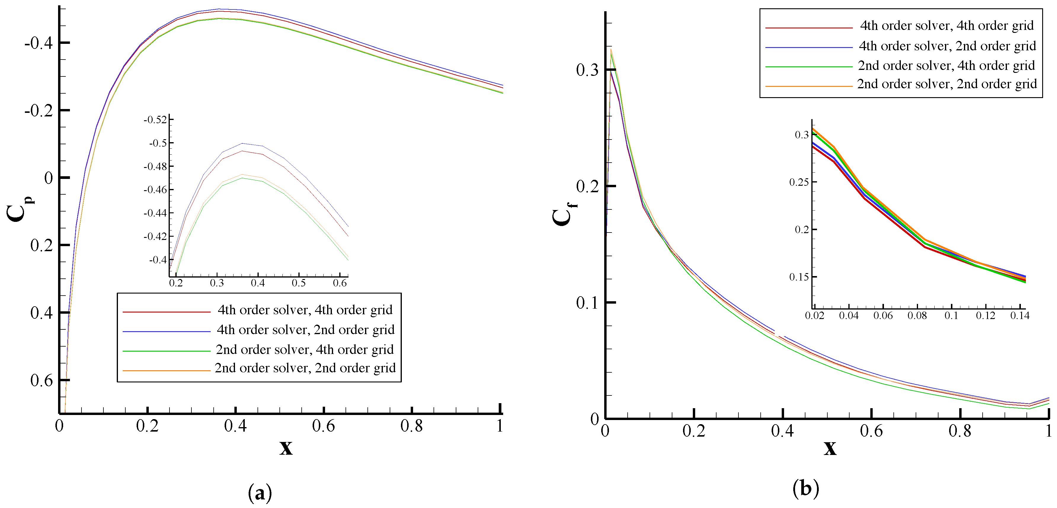
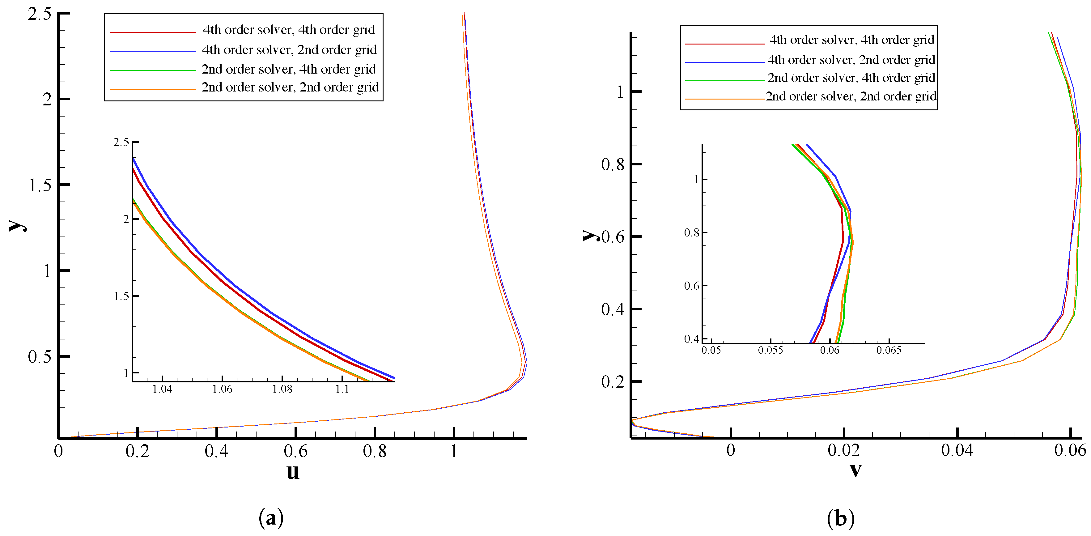
8. The Effect of the Grid Accuracy on Flow Solutions

In this section, we investigate the effects of grid accuracy on the numerical solutions of fluid flow around a NACA 0012 airfoil. The high-order compact flow solver was implemented in which the grid was generated through three different methods, including the standard second-order method, the compact scheme, and the Theodorsen technique. The distributions of pressure coefficient $C_p=2(p-p_{\infty })/\rho u_{\infty }^2$ and skin friction coefficient $C_f=2{\tau }_w/\rho u_{\infty }^2$ on the airfoil surface are respectively represented in Figure 11a,b for the subsonic, laminar flow (see, for example, [49,50,51]) with $Ma=0.5$ and $Re=10\times {10}^3$. The fourth-order compact grid generation method shows improvements in both pressure and skin friction coefficients compared to the second-order method and presents an excellent agreement with those results obtained from the Theodorsen grid generation technique. In addition to the subsonic flow, the supersonic flow over a NACA 0012 airfoil was also calculated. Figure 12 exhibits the pressure coefficient distributions for the inviscid supersonic flow with a Mach number of 1.2. Again, the zoomed-in views of this plot clearly demonstrate that the compact method agrees well with the Theodorsen method compared to the results of the second-order method. Although these figures indicate that there exists possibly an insignificant difference (approximately 5%, on average) between the results obtained from the second-order and the compact schemes, it is expected that the flow solutions are more affected by the grid accuracy for more complex geometries and turbulent flows [52,53].

As a final case, we examined the subsonic flow over the NACA 0012 airfoil but with $Ma=0.85$ and $Re=500$. Here, however, we employed the second-order flow solver in addition to the high-order compact solver to emphasize the importance of high-order solvers. The grid generation techniques remained the same as previous, i.e., second-order, fourth-order, and Theodorsen methods. Figure 13 and Figure 14 present the results of flow solutions for different flow solvers and grids. In general, the results of the high-order grid implemented with the high-order flow solver demonstrates a distinct difference compared to the results of the second-order grid coupled with the second-order solver. Moreover, the high-order compact finite-difference flow solver is more sensitive to the grid accuracy than the second-order solver. It can be argued that the truncation errors of the second-order flow solutions eliminate the effect of the grid accuracy. It can be inferred from Figure 13 that the pressure coefficient might be likely more susceptible to the accuracy of the flow solver than the skin friction coefficient. Finally, as shown in Figure 14, both horizontal and vertical velocity profiles present slight variations by either changing the accuracy of the grid generation technique or the flow solver.

9. Conclusions

In the present work, we presented a systematic numerical investigation to examine the influences of grid accuracy on the numerical solution of fluid flow problems with complex-shaped geometries. To this end, the flow field around a NACA 0012 airfoil was simulated using a high-order flow solver with various grid generation techniques. The grids around the NACA 0012 airfoil were generated using the standard second-order method and the fourth-order compact finite-difference scheme based on the elliptic approach. Moreover, following the Theodorsen approach, a conformal mapping is further employed to generate an orthogonal grid around the NACA 0012 airfoil. Here, a clear difference was observed between the grid metrics of the second- and fourth-order finite-difference schemes. Besides, compared to the Theodorsen’s orthogonal grid, the orthogonality of the grids generated by the fourth-order compact scheme is noticeably better than that of the second-order approach.

The effects of the grid accuracy on flow solutions were then evaluated for the flow fields around a NACA 0012 airfoil for which the computational grids were generated using the second-order, fourth-order compact, and Theodorsen schemes. The flow solvers were based on the standard second-order and fourth-order compact finite-difference methods. The results demonstrated that the accuracy of flow solutions are directly linked to the accuracy of the generated grids. In that regard, the grids generated using the fourth-order compact scheme showed improved results in comparison with grids generated by the second-order method. In particular, the pressure and skin-friction coefficients obtained from the numerical simulations with grids produced by the high-order compact method were well-matched with those obtained from Theodorsen conformal mapping. Furthermore, it was found that the fourth-order compact flow solver is more sensitive to the grid accuracy than the second-order one.

References

1. Soni, B.K. Grid generation: Past, present, and future. Appl. Numer. Math. 2000, 32, 361–369. [Google Scholar] [CrossRef]
2. Matsuno, K. High-order upwind method for hyperbolic grid generation. Comput. Fluids 1999, 28, 825–851. [Google Scholar] [CrossRef]
3. Vincent, P.E.; Jameson, A. Facilitating the adoption of unstructured high-order methods amongst a wider community of fluid dynamicists. Math. Model. Nat. Phenom. 2011, 6, 97–140. [Google Scholar] [CrossRef]
4. Wang, Z.; Fidkowski, K.; Abgrall, R.; Bassi, F.; Caraeni, D.; Cary, A.; Deconinck, H.; Hartmann, R.; Hillewaert, K.; Huynh, H.; et al. High-order CFD methods: Current status and perspective. Int. J. Numer. Methods Fluids 2013, 72, 811–845. [Google Scholar] [CrossRef]
5. Conti, C.; Morandi, R.; Spitaleri, R.M. On a mixed algebraic approach for generation and optimization of structured grids. In Proceedings of the 17th IMACS World Congress, Paris, France, 11–15 July 2005; pp. 1–8. [Google Scholar]
6. Gouin, M.; Ducrozet, G.; Ferrant, P. Propagation of 3D nonlinear waves over an elliptical mound with a high-order spectral method. Eur. J. Mech. B/Fluids 2017, 63, 9–24. [Google Scholar] [CrossRef]
7. Allahyari, M.; Mohseni, K. Numerical simulation of canonical shock/turbulence interaction using observable Navier-Stokes equations. Comput. Fluids 2020. Under Review. [Google Scholar]
8. Schaupp, C.; Sesterhenn, J.; Friedrich, R. On a method for direct numerical simulation of shear layer/compression wave interaction for aeroacoustic investigations. Comput. Fluids 2008, 37, 463–474. [Google Scholar] [CrossRef]
9. Emmett, M.; Zhang, W.; Bell, J.B. High-order algorithms for compressible reacting flow with complex chemistry. Combust. Theory Model. 2014, 18, 361–387. [Google Scholar] [CrossRef] [Green Version]
10. Allahyari, M.; Mohseni, K. Simulation of compressible flows and shock turbulence interaction using observable Euler and Navier-Stokes equations. Proceeding Aps Meet. Abstr. 2017, 62, A29.00006. [Google Scholar]
11. Allahyari, M.; Mohseni, K. Numerical simulation of flows with shocks and turbulence using observable methodology. In 2018 AIAA Aerospace Sciences Meeting; American Institute of Aeronautics and Astronautics: Kissimmee, FL, USA, 2018; p. AIAA 2018-0066. [Google Scholar] [CrossRef] [Green Version]
12. Lele, S.K. Compact finite difference schemes with spectral-like resolution. J. Comput. Phys. 1992, 103, 16–42. [Google Scholar] [CrossRef]
13. Laizet, S.; Lamballais, E. High-order compact schemes for incompressible flows: A simple and efficient method with quasi-spectral accuracy. J. Comput. Phys. 2009, 228, 5989–6015. [Google Scholar] [CrossRef]
14. Wang, Y.M.; Zhang, H.B. Higher-order compact finite difference method for systems of reaction–diffusion equations. J. Comput. Appl. Math. 2009, 233, 502–518. [Google Scholar] [CrossRef] [Green Version]
15. Brady, P.; Livescu, D. High-order, stable, and conservative boundary schemes for central and compact finite differences. Comput. Fluids 2019, 183, 84–101. [Google Scholar] [CrossRef] [Green Version]
16. Rahbari, I.; Paniagua, G. Acoustic streaming in turbulent compressible channel flow for heat transfer enhancement. J. Fluid Mech. 2020, 889, A2. [Google Scholar] [CrossRef]
17. Esfahanian, V.; Allahyari, M.; Hedayat, M. High order compact finite difference on multiblock domains with parallelization. In Proceedings of the 15th Conference on Fluid Dynamics, fd2013, Bandar Abbas, Iran, 18–20 December 2013. [Google Scholar]
18. Esfahanian, V.; Hedayat, M.; Baghapour, B.; Torabzadeh, M.; Hosseini, S. An Implicit Multigrid Solver for High-Order Compressible Flow Simulations on GPUs; APCOM & ISCM: Singapore, 2013. [Google Scholar]
19. Karman, S.L.; Erwin, J.T.; Glasby, R.S.; Stefanski, D. High-order mesh curving using WCN mesh optimization. In Proceedings of the 46th AIAA Fluid Dynamics Conference, Washington, DC, USA, 13–17 June 2016; p. AIAA 2016-3178. [Google Scholar]
20. Engvall, L.; Evans, J. Towards geometrically exact higher-order unstructured mesh generation. In Proceedings of the 25th International Meshing Roundtable, Washington, DC, USA, 26–30 September 2016. [Google Scholar]
21. Fortunato, M.; Persson, P.O. High-order unstructured curved mesh generation using the Winslow equations. J. Comput. Phys. 2016, 307, 1–14. [Google Scholar] [CrossRef] [Green Version]
22. Zhao, Z.; Li, M.; He, L.; Shao, S.; Zhang, L. High-order curvilinear mesh generation technique based on an improved radius basic function approach. Int. J. Numer. Methods Fluids 2019, 91, 97–111. [Google Scholar] [CrossRef]
23. Baker, T.J. Mesh generation: Art or science? Prog. Aerosp. Sci. 2005, 41, 29–63. [Google Scholar] [CrossRef]
24. Wang, J.; Zhong, W.; Zhang, J. A general meshsize fourth-order compact difference discretization scheme for 3D Poisson equation. Appl. Math. Comput. 2006, 183, 804–812. [Google Scholar] [CrossRef]
25. Shirayama, S. Effect of grid quality on the accuracy and convergency of computations. In Proceedings of the 13th Computational Fluid Dynamics Conference, Snowmass Village, CO, USA, 29 June–2 July 1997. [Google Scholar]
26. Farooq, M.A.; Müller, B. Accuracy assessment of the Cartesian grid method for compressible inviscid flows using a simplified ghost point treatment. J. Struct. Mech. 2011, 44, 279–291. [Google Scholar]
27. Karcz, J.; Kacperski, L. An effect of grid quality on the results of numerical simulations of the fluid flow field in an agitated vessel. In Proceedings of the 14th European Conference on Mixing, Warszawa, Poland, 10–13 September 2012; pp. 205–210. [Google Scholar]
28. Sankaranarayanan, S.; Spaulding, M.L. A study of the effects of grid non-orthogonality on the solution of shallow water equations in boundary-fitted coordinate systems. J. Comput. Phys. 2003, 184, 299–320. [Google Scholar] [CrossRef]
29. Bagade, P.M.; Bhumkar, Y.G.; Sengupta, T.K. An improved orthogonal grid generation method for solving flows past highly cambered aerofoils with and without roughness elements. Comput. Fluids 2014, 103, 275–289. [Google Scholar] [CrossRef]
30. Akcelik, V.; Jaramaz, B.; Ghattas, O. Nearly Orthogonal Two-Dimensional Grid Generation with Aspect Ratio Control. J. Comput. Phys. 2001, 171, 805–821. [Google Scholar] [CrossRef] [Green Version]
31. Huang, H.; Prosperetti, A. Effect of grid orthogonality on the solution accuracy of the two-dimensional convection-diffusion equation. Numer. Heat Transf. 1994, 26, 1–20. [Google Scholar] [CrossRef]
32. Putman, W.M.; Lin, S.J. Finite-volume transport on various cubed-sphere grids. J. Comput. Phys. 2007, 227, 55–78. [Google Scholar] [CrossRef]
33. Boyle, R.J.; Ameri, A.A. Grid orthogonality effects on predicted turbine midspan heat transfer and performance. J. Turbomach. 1997, 119, 31–38. [Google Scholar] [CrossRef]
34. Hefny, M.M.; Ooka, R. CFD analysis of pollutant dispersion around buildings: Effect of cell geometry. Build. Environ. 2009, 44, 1699–1706. [Google Scholar] [CrossRef]
35. Beam, R.M.; Warming, R.F. An implicit finite-difference algorithm for hyperbolic systems in conservation-law form. J. Comput. Phys. 1976, 22, 87–110. [Google Scholar] [CrossRef]
36. Douglas, J.; Gunn, J.E. A general formulation of alternating direction methods. Numer. Math. 1964, 6, 428–453. [Google Scholar] [CrossRef]
37. Janenko, N.N. The Method of Fractional Steps; Springer: Berlin/Heidelberg, Germany, 1971. [Google Scholar]
38. Zhang, X.; Blaisdell, G.A.; Lyrintzis, A.S. High-order compact schemes with filters on multi-block domains. J. Sci. Comput. 2004, 21, 321–339. [Google Scholar] [CrossRef]
39. Visbal, M.R.; Gaitonde, D.V. High-order-accurate methods for complex unsteady subsonic flows. AIAA J. 1999, 37, 1231–1239. [Google Scholar] [CrossRef]
40. Gaitonde, D.V.; Visbal, M.R. Pade-type higher-order boundary filters for the Navier-Stokes equations. AIAA J. 2000, 38, 2103–2112. [Google Scholar] [CrossRef]
41. Messiter, A.F. Boundary-layer flow near the trailing edge of a flat plate. SIAM J. Appl. Math. 1970, 18, 241–257. [Google Scholar] [CrossRef]
42. Bristeau, M.O.; Glowinski, R.; Periaux, J.; Viviand, H. Numerical Simulation of Compressible Navier-Stokes Flows: A GAMM-Workshop; Notes on Numerical Fluid Mechanics; Springer Science & Business Media: Braunschweig, Germany, 1987; Volume 18. [Google Scholar]
43. Arias, O.; Falcinelli, O.; Fico, N.; Elaskar, S. Finite volume simulation of a flow over a NACA 0012 using Jameson, MacCormack, Shu and TVD esquemes. Mec. Comput. 2007, 26, 3097–3116. [Google Scholar]
44. Shubin, G.; Stephens, A.; Glaz, H. Steady shock tracking and Newton’s method applied to one-dimensional duct flow. J. Comput. Phys. 1981, 39, 364–374. [Google Scholar] [CrossRef]
45. Joun, C.T.; Dale, A.A.; Richard, H.P. Computational Fluid Mechanics and Heat Transfer; Taylor & Francis: Gainesville, FL, USA, 1997. [Google Scholar]
46. Sorenson, S. A Computer Program to Generate Two-Dimensional Grids about Airfoils and Other Shapes by the Use of Poisson’s Equation; Technical Report NASA-TM-81198; NASA Ames Research Center: Moffett Field, CA, USA, 1980. [Google Scholar]
47. Theodorsen, T. Theory of Wing Section of Arbitrary Shapes; Technical Report NACA-TR-411; NACA Langley Aeronautical Lab: Langley Field, VA, USA, 1931. [Google Scholar]
48. Theodorsen, T.; Garrick, I.E. General potential theory of arbitrary wing sections. In Classical Aerodynamic Theory; Jones, R.T., Ed.; National Aeronautics and Space Administration: Moffett Field, CA, USA, 1979; pp. 257–290. [Google Scholar]
49. McMasters, J.H.; Henderson, M.L. Low speed single element airfoil synthesis. In Science and Technology of Low Speed and Motorless Flight; Hanson, P.W., Ed.; NASA Conference Publication: Hampton, VA, USA, 1979; pp. 1–31. [Google Scholar]
50. Yousefi, K.; Razeghi, A. Determination of the critical Reynolds number for flow over symmetric NACA airfoils. In Proceedings of the 2018 AIAA Aerospace Sciences Meeting, Kissimmee, FL, USA, 8–12 January 2018; p. AIAA 2018-0818. [Google Scholar]
51. Wang, J.; Nakata, T.; Liu, H. Development of mixed flow fans with bio-inspired grooves. Biomimetics 2019, 4, 72. [Google Scholar] [CrossRef] [PubMed] [Green Version]
52. Forrer, H.; Jeltsch, R. A higher-order boundary treatment for Cartesian-grid methods. J. Comput. Phys. 1998, 140, 259–277. [Google Scholar] [CrossRef]
53. Gullbrand, J.; Bai, X.S.; Fuchs, L. High-order Cartesian grid method for calculation of incompressible turbulent flows. Int. J. Numer. Methods Fluids 2001, 36, 687–709. [Google Scholar] [CrossRef]
Figure 1. Profiles of (a) horizontal velocity and (b) skin friction coefficient for flow over a flat plate with M a = 0.2 and R e = 200 × 10 3 . The results obtained from the Blasius boundary layer solution is also indicated by solid squares for comparison purposes.
Fluids 05 00110 g001
Figure 2. Profiles of (a) skin friction coefficient and (b) pressure coefficient over the NACA 0012 airfoil with M = 0.85 and R e = 500 . The results of the current numerical simulation are also compared with the reference solution of the GAMM-Workshop [42].
Fluids 05 00110 g002
Figure 3. Distribution of the pressure coefficient along the suction side of a NACA 0012 airfoil for inviscid flow with M = 1.2 . For comparison purposes, the results of Arias et al. [43] are also included.
Fluids 05 00110 g003
Figure 4. The supersonic flow inside a Shubin nozzle. (a) Pressure distribution along the nozzle length and its comparison with the exact solution, and (b) accuracy estimation of the fourth-order compact method.
Fluids 05 00110 g004
Figure 5. Schematic of the conformal transformation of planes in Theodorsen’s scheme [47,48].
Fluids 05 00110 g005
Figure 6. The grid generated in the area enclosed by two semicircles using the compact method.
Fluids 05 00110 g006
Figure 7. A comparison between the slope of the coordinate lines generated using the standard second-order and fourth-order compact methods and the orthogonal lines of the polar coordinate near the (a) lower and (b) upper boundaries of two semicircles.
Fluids 05 00110 g007
Figure 8. (a) O-type and (b) C-type grids generated around a NACA 0012 airfoil using different techniques, i.e., the fourth-order compact scheme, the Theodorsen’s scheme, and the standard second-order scheme.
Fluids 05 00110 g008
Figure 9. Comparison of the computational metrics (a) ξx and (b) ξy at x = 0.5 for the C-type grid.
Fluids 05 00110 g009
Figure 10. Comparison of the computational metrics (a) ξx and (b) ξy at x = 0.5 for the O-type grid.
Fluids 05 00110 g010
Figure 11. Comparison of the (a) pressure and (b) skin friction coefficients obtained using the fourth-order compact flow solver with different generated grids, including the standard second-order, compact fourth-order, and Theodorsen techniques, for flow around a NACA 0012 airfoil with M a = 0.5 and R e = 10 × 10 3 .
Fluids 05 00110 g011
Figure 12. Comparison of the pressure coefficient obtained using the fourth-order compact flow solver with different generated grids, including the standard second-order, compact fourth-order, and Theodorsen techniques, for inviscid flow around a NACA 0012 airfoil with M a = 1.2 .
Fluids 05 00110 g012
Figure 13. Comparison of the (a) pressure and (b) skin friction coefficients obtained using second- and fourth-order flow solvers with different generated grids for flow around a NACA 0012 airfoil with M a = 0.85 and R e = 500 .
Fluids 05 00110 g013
Figure 14. Comparison of the (a) horizontal and (b) vertical velocity components obtained using second- and fourth-order flow solvers with different generated grids for flow around a NACA 0012 airfoil with M a = 0.85 and R e = 500 .
Fluids 05 00110 g014