Study of Supercritical CO₂ Pipeline Flow Leaks: Effects of Equation of State, Impurity, and Outlet Diameter

Abstract

The growing need to mitigate climate change has accelerated the development of Carbon Capture, Utilization, and Storage (CCUS) technologies, where the safe transport of supercritical CO₂ (sCO₂) through pipelines is a key challenge. The flow behavior in such systems is strongly influenced by phase-change processes under transient conditions such as decompression and heat transfer and is further complicated by the presence of impurities (e.g., N₂, CH₄, and Ar). These impurities modify thermodynamic properties and phase boundaries, thereby affecting the overall flow dynamics. In this study, the influence of impurities on leakage, mass flow rate, and decompression wave propagation in sCO₂ pipelines is investigated using computational fluid dynamics (CFD) simulations. A real-fluid model (RFM) implemented in the CONVERGE CFD solver is employed, with a tabulation-based approach to accurately capture thermodynamic and transport properties across multiphase regimes. The simulations were validated against available experimental data and performed for varying impurity concentrations to assess their impact on key flow variables, including pressure, temperature, and wave speed. Although simplifying assumptions were used, the results are in fairly good agreement with experimental observations and provide a better understanding of the phase behavior induced by impurities during transient decompression. Additionally, the effects of outlet geometry, pipeline configuration, and the choice of equation of state are examined, highlighting their influence on the predicted flow response. The validity of the RFM modeling framework is further demonstrated by simulations of a large-scale pipeline configuration representative of industrial conditions, which will serve as a benchmark for future improvements.

1. Introduction

The past decade has witnessed a significant expansion of CO₂ pipeline networks globally, driven by the growing emphasis on carbon capture, utilization, and storage (CCUS) initiatives; applications in enhanced oil recovery (EOR); and the aim to reduce anthropogenic CO₂ emissions and meet global de-carbonization targets [1,2]. Recently, significant progress has been made in CCUS technologies [3,4,5], and it has been found that systems perform efficiently when the fluid (CO₂) is in a supercritical state (sCO₂). Thus, the accurate modeling of supercritical carbon-dioxide (sCO₂) transport becomes increasingly important for the design, safety assessment, cost reduction, and operational reliability of pipeline and storage systems in CCUS [6,7,8]. One of the critical questions in the safety assessment of sCO₂ transport systems pertains to the mass flow rate during depressurization or leakage, which is strongly influenced by decompression wave speed and mixture impurities. Non-equilibrium phase change retarded by nucleation and vapor-front dynamics is found to have significant effects, but only during the early leakage stage (few milliseconds) [9,10,11]. Consequently, metastability phenomena (i.e., non-equilibrium thermodynamics) are neglected in this article, as we intend to perform CFD simulations over significantly longer periods of time. Early work by Mahgerefteh et al. [12] employed 1D models to investigate the influences of friction, heat transfer, and stream impurities on decompression wave speeds in sCO₂ pipelines. Subsequent studies by Woolley et al. [6,13,14] combined experimental and numerical approaches to analyze multi-component CO₂ mixtures, providing foundational data for safety guidelines. Recent reviews [15,16,17,18] have discussed challenges in accurately modeling the decompression wave, thermophysical properties, phase equilibria, and dispersion of CO₂ and its mixtures. Shuaiwei et al. [19] showed that an isentropic assumption during depressurization predicts the decompression wave speed for CO₂ and its mixtures quite accurately. Similarly, Magen et al. [20], assuming an isentropic phase change, provided a formulation for predicting the onset of nucleation by estimating the minimum depressurization rate near the spinodal limit. Using experimental data, Xiaoqiang et al. [21] correlated the non-dimensional depressurization rate with the degree of superheating. Liao et al. [22] analyzed the critical-mass flux and decompression wave speed for CO₂ and its mixtures through 1D analysis using different models and provided a correlation for the mass flow rate. Cao et al. [23] focused on the flow field in pipe cross-sections and described the stratification of phases during pressure leakage. Hansen et al. [24,25] analyzed the problem in a vertical pipe duct and estimated reference data for a 1D phase transition model. Bhuvanker et al. [26] studied the effects of heat transfer and gravity in CO₂ blowout. Yin et al. [27] studied the depressurization phenomenon numerically using a homogeneous equilibrium model (HEM) and a homogeneous relaxation model (HRM). Log et al. [28] and Wang et al. [29] proposed correlations for the HRM relaxation time based on initial entropy. Log et al. [30] proposed a model to include the effects of nucleation and bubble growth in the source for mass transfer. Munkejord et al. [31] and Yu et al. [32] studied the effect of impurities for CO₂-N₂ mixtures. Zhu et al. [33] analyzed the effect of water hammering on phase transition for pipeline transport. Lio et al. [34] proposed a neural network model to predict critical mass flow. Yu et al. [35] studied the depressurization phenomenon during multistage throttling. While previously discussed research was conducted for pressure puncture, many studies have also been done on orifice leakage. Ding et al. [36] proposed a pressure correction procedure for estimating the corrected leakage rate. Zhang et al. [37] analyzed the near-field characteristics for sCO₂ during pressure leakage and proposed an empirical correlation of saturation pressure ($P_{sat}$) for numerical modeling. Yu et al. [38] studied the temperature distribution and CO₂ dispersion for a pipe leak buried in soil. Similarly, in [39], they analyzed the problem numerically using a leakage and seepage diffusion model. Chen et al. [40] analyzed the effect of orifice diameter; similarly, Hu et al. [41] analyzed the effect of orifice diameter for underwater pipeline leakage.

The numerical modeling of operations close to the supercritical state poses a number of challenges, the first of which is the non-linear behavior of thermodynamic and transport properties [17,32] near the critical point. A further complicating factor is the presence of impurities such as H₂O, N₂, H₂, CH₄, O₂, H₂S, SO_x, and NO_x, which significantly alter mixture thermodynamics and transport properties. Pure CO₂ can be accurately modeled using multi-parameter equations of state (EoSs) like that proposed by Span and Wagner [42], but such equations are computationally expensive. Nazeri et al. [43] demonstrated that incorporating a volume correction term into the Soave–Redlich–Kwong (SRK) EoS enhances density predictions for CO₂-rich mixtures. Similarly, Demetriades et al. [44] derived a pressure-explicit EoS for CO₂-N₂-O₂-H₂ systems, which outperformed the GERG-2008 model [45] in certain regimes. Petropoulou et al. [46] further compared various EoSs with Universal Mixing Rules (UMRs) for CO₂/CH₄ mixtures, finding that the Peng–Robinson (PR) EoS provided the best VLE predictions. Similarly, Li and Yan [47] analyzed five different cubic EoSs for VLE calculations of CO₂ and CO₂ mixtures. Diamantonis et al. [48] compared SAFT and PC-SAFT [49] with cubic EoSs for VLE modeling of CO₂ mixtures. Avendano et al. [50] presented a parameter set for the SAFT-$\gamma$ model [51] for CO₂. Accurate prediction of transport properties (e.g., viscosity and thermal conductivity) remains another key hurdle. While empirical correlations like those of Bahadori and Vuthaluru [52] and Nazeri et al. [53] have improved viscosity estimates for CO₂-rich mixtures, thermal conductivity modeling relies heavily on correlations such as those proposed by Jarrahian and Heidaryan [54] and Rostami et al. [55]. Cross-property interactions such as those studied by Hellmann et al. [56] using the classical trajectory method further complicate the picture. A persistent challenge is the scarcity of high-quality experimental data [57], which limits the validation and refinement of these models. The nonlinearities introduced by real-fluid EoSs and phase-change phenomenon increases the numerical stiffness of the system as well. This severely affects the stability and convergence of solvers, consequently raising the computational cost. Modeling of the formation of dry ice, which is very common for the case of sCO₂ depressurization, is another challenge. An accurate EoS model of solid CO₂ is needed. Trusler [58] and Jager and Span [59] proposed a Helmholtz and Gibbs energy-based model for solid CO₂, respectively. These models have been validated for various systems [60,61,62] and found to be reasonably accurate in experiments. Maltby [63] reviewed various experimental data for various CO₂ systems and found that the deviation is minimal with PR EoSs considering the overall range of various conditions. Bhatia et al. [64] found that CPA outperforms PR for the case of condensation of CO₂ through a convergent–divergent nozzle. The unsuitability of the PR EoS method when applied to the modeling of pipeline decompression was also highlighted by Flechas et al. (2020) [65], particularly because it significantly underestimates the speed of sound. Aursand et al. (2016) [66] demonstrated that impurities significantly increase the saturation pressure and cricondenbar, with implications for ductile fractures and the operating pressure. These observations motivate a more detailed investigation using recent transient CFD solvers of the influence of the EoS and CO₂ mixture composition on simulations of transient pipeline decompression. The impact of impurities and EoS accuracy were also highlighted by Vitali et al. (2023) [67], who showed that GERG-type EoSs are generally more accurate in the description of both vapor–liquid equilibrium (VLE) and density when compared with cubic EoSs. GERG-type EoSs are found to be more accurate for light component systems like CO₂+impurities. However, such an EoS is less versatile than a cubic EoS (like CPA and SRK) and involves many more parameters for each component and binary system. The overestimated predictions, with an average of up to 4.5% for PR and CPA, could be considered acceptable in the context of our current study for computational cost reasons, as the aim is solely to evaluate our new real-fluid model (RFM) [64,68,69,70,71] recently implemented in the CONVERGE solver [72], not only for CCUS pipeline applications. While previous studies have extensively investigated the accuracy of various EoSs for the prediction of thermophysical properties and phase equilibria of CO₂ and CO₂-rich mixtures, most of these analyses are conducted in isolation from the underlying flow dynamics. In particular, the impact of EoS selection on transient decompression behavior, including wave propagation, phase-transition dynamics, and the leakage mass flow rate, remains less explored within fully coupled transient CFD frameworks. In the practical analysis of pipeline safety, the choice of EoS influences the equilibrium properties and, consequently, directly affects the compressibility, density, speed of sound, and phase-envelope accuracy, which, in turn, determine the speed of the decompression wave and the critical discharge conditions. Therefore, a systematic assessment of available EoS performance within a transient, multidimensional CFD framework is essential for bridging the gap between thermodynamic modeling and engineering-scale predictions.

Despite the substantial body of work summarized above, several important limitations remain. Most existing investigations rely predominantly on one-dimensional, homogeneous equilibrium or relaxation models to predict decompression wave speeds and critical mass flux. While these approaches provide valuable theoretical insight and are computationally efficient, they inherently neglect multidimensional flow structures, spatial phase stratification, and local non-uniformity arising during realistic pipeline leakage. Furthermore, many studies emphasize either thermodynamic modeling or empirical correlations independently, with limited integration into fully coupled CFD frameworks capable of resolving transient flow–thermodynamics interactions over engineering time scales. In addition, although the influence of impurities has been recognized, systematic numerical investigations incorporating real-fluid equations of state, together with transport-property variations, remain scarce. The combined effects of non-linear thermophysical behavior near the critical region, phase change, and stiff source terms pose significant challenges for stable and efficient numerical solvers, which has limited the application of high-fidelity CFD to practical large-scale problems. Consequently, there is still a lack of robust, computationally tractable models that can accurately predict depressurization dynamics and mass discharge rates for realistic multi-component CO₂ mixtures over extended transient periods relevant to safety assessment and pipeline design. The present work aims to address these gaps by developing and applying a CFD-based framework that incorporates real-fluid thermodynamics, mixture-dependent properties, and transient multiphase effects to systematically evaluate decompression behavior and leakage characteristics of CO₂ pipelines under practical operating conditions. In the present work, a high-fidelity Real-Fluid Method (RFM) solver implemented in CONVERGE CFD v4.1 is used. The framework is validated for real gas-evaporating and non-evaporating sprays [73,74,75]. The thermophysical properties are calculated by a robust thermodynamic solver developed at IFP Energies Nouvelle [76]. Model validation leverages high-resolution experimental pressure–temperature data from Munkejord et al. [31,77,78], providing a rigorous benchmark for assessing accuracy. The selected binary systems are CO₂-N₂, CO₂-CH₄, and CO₂-Ar, representing the major non-condensable impurities relevant to current and emerging sCO₂ capture, transport, and storage applications [79]. The key contributions of this work are:

• A critical assessment of the influence of the equation of state on the prediction of thermophysical properties for sCO₂ and its mixtures;
• Depressurization analysis of the flow rate, pressure depression, and void-fraction profiles with different outlet diameters and geometries for CO₂-rich mixtures;
• An evaluation of the effect of impurities on decompression wave propagation and the resulting critical mass flow rate by simulating a binary mixture.

The following sections detail the numerical methodology (Section 2), as well as computational setup and mesh sensitivity study (Section 3). Results and discussions (Section 4) include the validation of the CPA EoS and VLE thermodynamic equilibrium. The effect of impurities is studied in detail for various parameters of concern in the pipeline industry. Section 4 also compares the simulated pressure profile, gas-fraction variations, and the thermodynamic path against experimental benchmarks. The effects of impurities on the decompression wave speed, mass flow rate, and Mach number are also discussed. Section 5 presents an exploratory study of supercritical CO₂ pipeline transport at industrial scale. Finally, the Conclusion discusses key findings and highlights the broader implications of impurity-sensitive modeling for the design and transient safety assessment of industrial-scale sCO₂ transport systems.

2. Numerical Methodology

2.1. Governing Equations

The mixture is represented as a single effective fluid in which the two phases share identical velocity, pressure, and temperature fields. Accordingly, the formulation reduces to four governing equations [68,69,70,71]:

$${\displaystyle \frac{\partial \rho }{\partial t}}+{\displaystyle \frac{\partial \rho u_i}{\partial x_i}}=0$$

(1)

$${\displaystyle \frac{\partial \rho u_i}{\partial t}}+{\displaystyle \frac{\partial \rho u_i{u}_j}{\partial x_j}}=-{\displaystyle \frac{\partial P}{\partial x_i}}+{\displaystyle \frac{\partial }{\partial x_j}}\left({\tau }_{ij}+{\tau }_{ij}^{SGS}\right)$$

(2)

$${\displaystyle \frac{\partial \rho e}{\partial t}}+{\displaystyle \frac{\partial \rho e{u}_j}{\partial x_j}}=-P{\displaystyle \frac{\partial u_j}{\partial x_j}}+\left({\tau }_{ij}+{\tau }_{ij}^{SGS}\right){\displaystyle \frac{\partial u_i}{\partial x_j}}+{\displaystyle \frac{\partial }{\partial x_j}}\left(q_j+q_j^{SGS}\right)$$

(3)

$${\displaystyle \frac{\partial \rho Y_k}{\partial t}}+{\displaystyle \frac{\partial \rho Y_k{u}_j}{\partial x_j}}=-{\displaystyle \frac{\partial }{\partial x_j}}\left(J_{kj}+J_{kj}^{SGS}\right)$$

(4)

where $\rho$, u, P, T, and e denote the mixture density, velocity, pressure, temperature, and specific internal energy. The molecular viscous stress tensor is given by

$${\tau }_{ij}=\mu \left({\displaystyle \frac{\partial u_i}{\partial x_j}}+{\displaystyle \frac{\partial u_j}{\partial x_i}}-{\displaystyle \frac{2}{3}}{\displaystyle \frac{\partial u_k}{\partial x_k}}{\delta }_{ij}\right),$$

(5)

with ${\delta }_{ij}$ representing the Kronecker delta.

The heat flux and diffusive flux of species are expressed as

$$q_j=-\lambda {\displaystyle \frac{\partial T}{\partial x_j}}+\sum _m{J}_{mj}{h}_m,J_{mj}=-\rho D_m{\displaystyle \frac{\partial Y_m}{\partial x_j}}$$

(6)

where $h_m$ is the species enthalpy, $D_m$ is the molecular diffusivity, and $Y_m$ is the mass fraction of species m. The transport coefficients ($\mu$ and $\lambda$) are obtained from the correlations of Chung et al. [80].

The subgrid-scale (SGS) stresses and fluxes are modeled by analogy with molecular terms. The SGS stress tensor is

$${\tau }_{ij}^{SGS}={\displaystyle \frac{{\mu }^{SGS}}{\mu }}{\tau }_{ij},$$

(7)

while the turbulent contributions to heat and mass transfer are

$$q_j^{SGS}=-{\lambda }_t{\displaystyle \frac{\partial T}{\partial x_j}}+\sum _m{J}_{mj}^{SGS}{h}_m,J_{mj}^{SGS}=-\rho D_{mt}{\displaystyle \frac{\partial Y_m}{\partial x_j}}$$

(8)

The turbulent transport properties are modeled as

$$D_{mt}={\displaystyle \frac{{\mu }_{SGS}}{\rho S{c}_t}},{\lambda }_t={\displaystyle \frac{C_p{\mu }_{SGS}}{P{r}_t}}$$

(9)

with $S{c}_t=0.7$, $P{r}_t=0.9$, and $C_p$ representing the specific heat at constant pressure. The eddy viscosity (${\mu }_{SGS}$) follows the $\sigma$ model [81], i.e.,

$${\mu }_{SGS}=\rho {\left(C\mathsf{\Delta }\right)}^2\delta$$

(10)

where $C=1.5$, $\mathsf{\Delta }=V^{1/3}$, V is the grid-cell volume, and $\delta ={\displaystyle \frac{{\sigma }_3({\sigma }_1-{\sigma }_2)({\sigma }_2-{\sigma }_3)}{{\sigma }_1^2}}$ using the singular values (${\sigma }_i$) of the resolved velocity-gradient tensor. In this work, cross-coupling effects such as Soret and Dufour are neglected.

2.2. Thermodynamic Modeling

The Real-Fluid Method (RFM) [68,69,70,71] is based on tabulated thermodynamic data generated using the IFPEN-Carnot library [76]. The library applies PT-flash calculations for mixtures and PH-flash for pure fluids, with different cubic and association EoSs (PR [82], CPA [83], and PC-SAFT [49]). Flashing involves a stability test (tangent-plane distance criterion) followed by phase-split determination.

The lookup tables, discretized in $(T,P,Y_k)$ for mixtures (or $(h,P)$ for pure fluids), provide the equilibrium density, internal energy, vapor fraction, heat capacity, sound speed, and transport properties. Property queries are interpolated via Inverse Distance Weighting (IDW) [84]. This methodology has been successfully applied to binary [73,75,85] and ternary [74] mixtures and is implemented in CONVERGE CFD [86].

The tables are used during runtime for:

• Property evaluation as a function expressed as $f(T,P,Y_k)$;
• Reverse lookup ($T=f(e,P,Y_k)$) after solving for internal energy.

Because of the non-linear behavior of real-fluid EoSs, the standard pressure equation must be reformulated. A pressure–density ratio is defined locally for each cell and time step to incorporate the effects of real fluid compressibility as

$${\varphi }^{\ast }={\left({\displaystyle \frac{\partial \rho }{\partial p}}\right)}_{T,Y}.$$

(11)

Within the PISO loop, the pressure equation reads

$${\displaystyle \frac{{\partial }^2(P^{\ast \ast }-P^{\ast })}{\partial x_i\partial x_i}}-{\displaystyle \frac{{\varphi }^{\ast }(P^{\ast \ast }-P^{\ast })}{d{t}^2}}={\displaystyle \frac{({\rho }^{Eo{S}^{\ast }}-{\rho }^n)}{d{t}^2}}+{\displaystyle \frac{1}{dt}}\left({\displaystyle \frac{\partial {\rho }^{\ast }{u}_i^{\ast \ast }}{\partial x_i}}-S\right)$$

(12)

where ** and * refer to successive PISO iterations, ^EoS designates the density obtained from the table, and ⁿ indicates the current time step. Although no explicit phase-change source terms are included in the transport equations under equilibrium, mass and energy transfer are consistently handled via property lookup and reverse-lookup procedures. A similar procedure is used for single-component CO₂ simulations, where the table inputs are ($h,P$). In this case, h is evaluated as ($e+P/\rho$), and the temperature is among the outputs in the table.

2.3. Numerical Schemes

The spatial discretization uses a first-order accurate Euler upwind scheme. Time integration is performed using a first-order explicit Euler forward scheme. This treatment enhances numerical robustness during the highly transient depressurization phase while maintaining computational efficiency. A dynamically adaptive time-stepping strategy is adopted. During the initial stage of depressurization, where the flow is strongly shock-dominated and characterized by steep pressure gradients, the time step is on the order of $\mathcal{O}\left(10\mathrm{ns}\right)$. As the flow transitions beyond the choked regime and pressure gradients relax, the time step is gradually increased up to $\mathcal{O}\left(10\mathrm{ms}\right)$. Numerical stability is primarily governed by shock propagation and rapid pressure-wave dynamics. The maximum allowable time step is controlled using a Courant–Friedrichs–Lewy (CFL) criterion based on the local Mach number. The maximum CFL number attained at maximum $dt$ is 2.0 for laboratory-scale pipeline simulations and 8.0 for industrial-scale pipeline configurations. The larger permissible CFL number in industrial-scale cases is attributed to the longer characteristic length scales and comparatively smoother spatial gradients following the initial decompression-front propagation. All simulations are performed on AMD EPYC Genoa 9534 processors operating at 2.45 GHz on the ORION super-computing cluster, BULL, France. A total of 128 cores are used for lab-scale pipeline flow, and 256 cores are used for the industrial-scale pipeline flow. Thermodynamic closure within the RFM framework is provided by the CPA EoS. Thermodynamic properties are evaluated using pre-tabulated data with a resolution of

$$\mathsf{\Delta }T=1\mathrm{K},\mathsf{\Delta }P=0.1\mathrm{bar},\mathsf{\Delta }Y=\mathrm{Impurity}\mathrm{mass}\mathrm{fraction}.$$

(13)

The selected tabulation resolution is consistent with prior validation studies [64,69,70,71,75], ensuring an appropriate balance between interpolation accuracy and computational cost for multi-component CO₂ mixture depressurization simulations.

3. Computational Setup

3.1. Setup Description

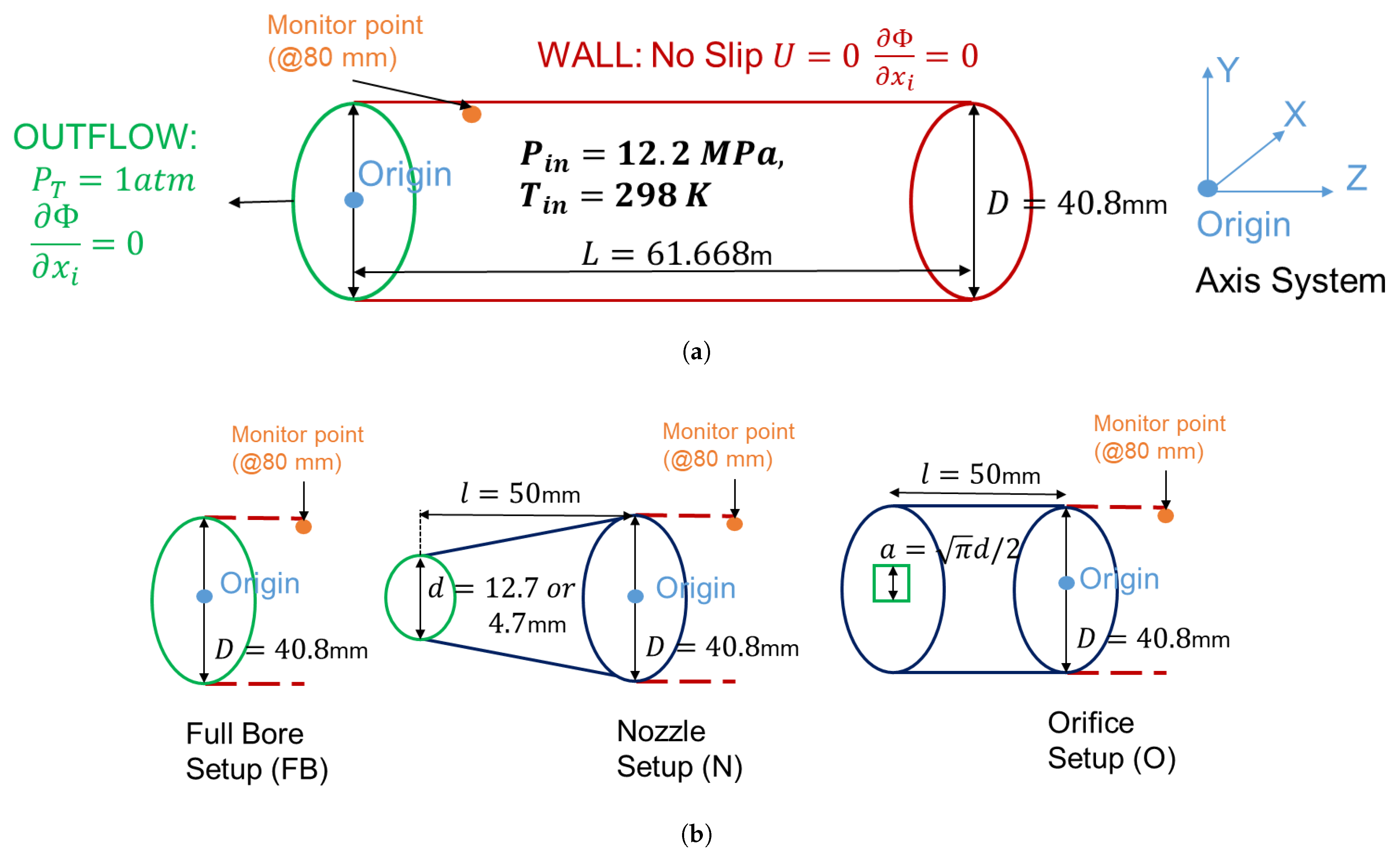
The computational domain is shown in Figure 1. It is a cylindrical pipe with a diameter of $D=40.8$ mm and a length of $L=61.7$ m, which are parameters relevant to the experimental setup of Munkejord et al. [31,77]. The domain has two boundaries. First, the OUTLET plane is located on the left side, which is the location of the disk rupture (simulating the leak), and the remaining boundaries are defined as WALL. Hence, the boundary conditions are Dirichlet conditions for pressure and Neumann conditionsfor the rest of the depending variables, such as the temperature and velocity at the outlet. The outlet pressure is defined by the atmospheric condition, with total pressure as 1 atm ($P_{amb}=0.1325$ MPa). At the wall, no slip condition is imposed. The temperature is assumed to remain constant at the wall throughout the simulation, i.e., $T_{wall}=T_0=298$ K. The pipe is initially filled with sCO₂ in a liquid-like state, as the initial condition inside the pipeline is defined by the fluid thermodynamic state ($T_0=298$ K) and $(P_0=12.27$ MPa), which is greater than the critical pressure ($P_c=7.3773$ MPa) of pure CO₂. The disk ruptures at time $t=0$, and liquid-like sCO₂ inside the pipe is exposed to atmospheric conditions ($P_{amb}=0.1325$ MPa, $T_{amb}=277$ K), causing a two-phase boiling shock including a sudden expansion wave with a violent phase change. The initial and atmospheric conditions remain the same for all the cases. The test matrix is designed to systematically assess the influence of the EoS, impurities, outlet geometry, and diameter. The test matrices for the present study are shown in

Table 1. Test matrix for depressurization simulations of supercritical CO₂–N₂ mixtures, highlighting the influence of the EoS.

Case ID	EoS	Outlet Type	Impurity (mol%)	Impurity (mass%)
C1 (No. 9 [31])	CPA	FB	N2 (1.8)	N2 (1.15)
C2 (No. 9 [31])	PR	FB	N2 (1.8)	N2 (1.15)
C3 (No. 9 [31])	SAFT	FB	N2 (1.8)	N2 (1.15)

EoS abbreviations: PR—Peng–Robinson; CPA—Cubic-Plus-Association; SAFT—Statistical Associating Fluid Theory. Outlet-type abbreviations: FB—Full bore with a 40.8 mm diameter.

,

Table 2. Test matrix for depressurization simulations of supercritical CO₂ mixtures, highlighting the influence of impurities.

Case ID	EoS	Outlet Type	Impurity (mol%)	Impurity (mass%)
C4	CPA	FB	N2 (3.6)	N2 (2.3)
C5	CPA	FB	N2 (5.4)	N2 (3.5)
C6	CPA	FB	CH4 (3.6)	CH4 (1.3)
C7	CPA	FB	CH4 (5.4)	CH4 (2.0)
C8	CPA	FB	Ar (3.6)	Ar (3.2)
C9	CPA	FB	Ar (5.4)	Ar (4.9)

EoS abbreviations: PR—Peng–Robinson; CPA—Cubic-Plus-Association; SAFT—Statistical Associating Fluid Theory. Outlet-type abbreviations: FB—Full bore with a 40.8 mm diameter.

and

Table 3. Test matrix for depressurization simulations of supercritical CO₂+N₂ mixture, highlighting the influence of outlet geometry and diameter.

Case ID	EoS	Outlet Type	Impurity (mol%)	Impurity (mass%)
C10 (No. 13 [78])	CPA	O (12.7 mm)	N2 (1.8)	N2 (1.15)
C11 (No. 16 [78])	CPA	O (4.5 mm)	N2 (1.8)	N2 (1.15)
C12 (No. 18 [78])	CPA	N (12.7 mm)	N2 (1.8)	N2 (1.15)
C13 (No. 17 [78])	CPA	N (4.5 mm)	N2 (1.8)	N2 (1.15)

EoS abbreviations: CPA—Cubic-Plus-Association. Outlet-type abbreviations: O—Orifice; N—Nozzle.

. In addition to these test cases, a reference case (C0) of pure CO₂ is also studied; the initial and atmospheric conditions are similar, i.e., ($P_0=12.22$ MPa, $T_0=297.6$ K) and ($P_{amb}=0.1325$ MPa, $T_{amb}=281$ K) [77]. The geometry for cases C10–C13 are taken from [78] and are schematically shown in Figure 1b. The new outlet plane for these cases is at a distance of $l=50$ mm from the previous outlet plane, and the boundary area is varied through d, the diameter of the orifice or nozzle. For the case of an orifice, a rectangular instead of circular boundary is chosen, keeping the geometry and net outlet boundary area identical, as depicted in Figure 1b. This point will be discussed again in Section 4.4. Fluid impurities and initial conditions are selected to provide detailed information relevant to IFPEN’s current projects. The various parameters used in the IFPEN-Carnot [76] thermodynamic solver for calculation of the thermophysical properties are summarized in

Table 4. Parameters used for calculation of thermophysical properties in IFPEN-Carnot [76]. $T_{min}$ and $T_{max}$ are the minimum and maximum temperature values required. $P_{min}$ and $P_{max}$ are the minimum and maximum pressure values required. $Y_{min}$ and $Y_{max}$ are the minimum and maximum mass fraction values required.

Mixture	Flash Type	${\mathit{T}}_{\mathit{min}}$ (in K)	${\mathit{T}}_{\mathit{max}}$ (in K)	Nsteps (for T)	${\mathit{P}}_{\mathit{min}}$ (in Bar)	${\mathit{P}}_{\mathit{max}}$ (in Bar)	Nsteps (for P)	${\mathit{Y}}_{\mathit{min}}$	${\mathit{Y}}_{\mathit{max}}$	Nsteps (for Y)
Pure CO2	PH	130	310	180	0.1	130.1	1301	-	-	-
CO2+N2	PT	130	310	180	0.1	130.1	1301	0	1	1/ΔY
CO2+CH4	PT	190	310	120	0.1	130.1	1301	0	1	1/ΔY
CO2+Ar	PT	110	310	200	0.1	130.1	1301	0	1	1/ΔY

.

3.2. Mesh Sensitivity

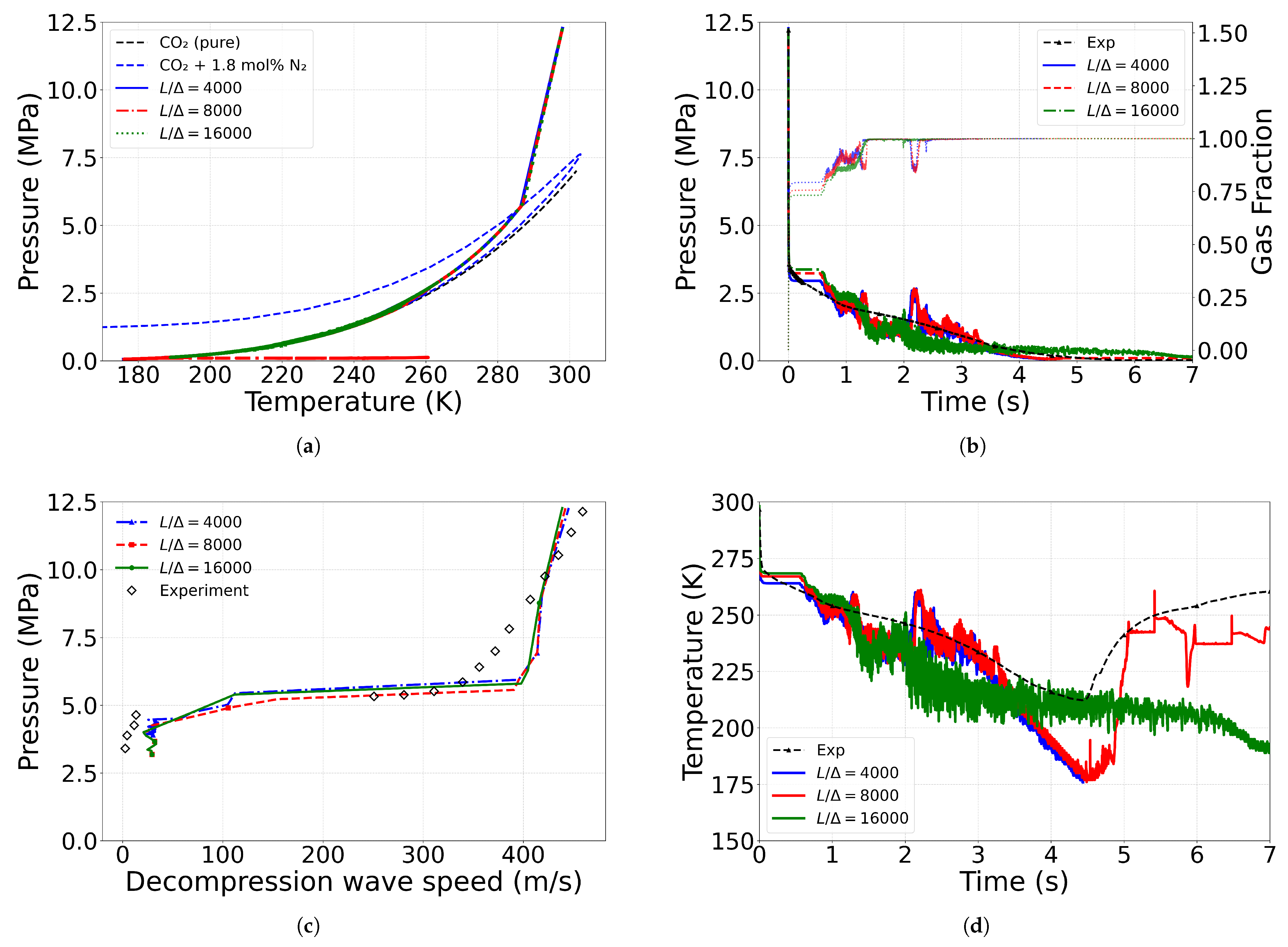
The mesh sensitivity is determined for the Case C1 in Table 1. A uniform 1D-like mesh is used for all the cases in the present work, with four fixed cells in the cross-section, i.e., ${\mathsf{\Delta }}_x={\mathsf{\Delta }}_y=20.4$ mm, and refined in the axial (z) direction, making the setup almost a 1D setup. A minimum cross-sectional resolution (four cells) is needed to adequately define the geometry and boundary conditions within the finite volume framework while focusing on the dominant axial flow dynamics. The mesh sensitivity is analyzed with three different mesh resolutions i.e., $L/{\mathsf{\Delta }}_z$ = 4000, 8000, and 16,000, corresponding to ${\mathsf{\Delta }}_z\approx 16,8$, and 4 mm and approximately $14.8,29.6$, and $59.2$ thousands of cells. The results are analyzed through a monitor point at a distance of $x=80$ mm, as shown in Figure 1, which corresponds to the normalized distance ($x/D\approx 2$) for case C1. The grid-sensitivity results are depicted in Figure 2. Apart from grid sensitivity, the result also validates the numerical model with experimental data. The error percentage in the pressure and gas volume fraction profile is less than 10% before the fluctuation in properties begins due to phase transition and local changes in the mach number but also due to the interactions with reflected pressure waves at the pipeline’s closed end on the right side. The computational resources taken for five seconds of runtime at different mesh resolutions are given in

Table 5. Computational time taken for the different mesh resolutions and five seconds of runtime in Case C1.

$\mathit{L}/{\mathbf{\Delta }}_{\mathit{z}}$	4000	8000	16,000
Total number of cells	4800	29,600	59,200
Computational time (hrs)	3.24	6.29	20.7
Node/core numbers	1/128	1/128	1/128

.

The decompression process considered in the present study is predominantly governed by axial pressure-wave propagation, with limited transverse flow development, except in the near-outlet region. This justifies the use of a quasi-one-dimensional discretization with a coarse cross-sectional resolution, enabling computational efficiency while retaining the dominant physics and in line with previous studies in the literature [28,30]. The grid-sensitivity results (Figure 2) further demonstrate that additional axial refinement does not lead to significant changes in the evolution of primary variables such as pressure and gas fraction, which control the decompression dynamics. Consequently, derived quantities, including the decompression wave speed and mass flow rate, remain consistent across grid levels. It is acknowledged that for cases involving complex outlet geometries, a fully resolved three-dimensional discretization may be required to capture localized flow features with higher fidelity. However, within the scope of the present study, the adopted mesh provides physically consistent and quantitatively reasonable predictions when compared with experimental observations, without introducing significant deviations in the key flow characteristics. Furthermore, a preliminary assessment was conducted for the CO₂+N₂ (3.6% mol) mixture (Case C4) using both rectangular and circular geometries. The results from the two configurations show good agreement over the relevant time scales, supporting the validity of the geometric assumption adopted in the present study. Temporal resolution is ensured through an adaptive time-stepping strategy based on a CFL condition, where the time step varies from $\mathcal{O}\left(10\mathrm{ns}\right)$ during the initial shock-dominated regime to $\mathcal{O}\left(10\mathrm{ms}\right)$ in the later stages. This ensures accurate resolution of rapid transients while maintaining computational efficiency over the full simulation duration. A detailed uncertainty analysis is presented in the next section to further strengthen the adequacy of the mesh resolution with $L/{\mathsf{\Delta }}_z=8000$ for the present study.

3.3. Uncertainty Analysis

The results presented in Figure 2a demonstrate that, owing to the highly coupled nature of the flow solver and the thermodynamic solver (see Section 2.2, the framework is able to accurately capture the thermodynamic path, even with relatively coarse grid resolutions. This capability is primarily attributed to the use of a consistent, high-resolution thermophysical property table across all grid configurations, ensuring uniform representation of thermodynamic states, irrespective of spatial discretization (Equation (13) and Table 4). Figure 2b–d further illustrate the evolution of the pressure, gas fraction, decompression wave speed, and temperature profiles. The methodology used to determine the decompression wave speed is described in detail in Section 4. To quantify the influence of mesh resolution on key flow and thermodynamic variables, a discretization uncertainty analysis based on the Grid Convergence Index (GCI) methodology [87] is performed. The analysis is conducted using discrete temporal sampling, with 20 representative points selected over the interval of t = 0–1.2 s. This interval corresponds to the physically most relevant regime of the decompression process, where rapid pressure evolution, phase transition, and peak mass discharge occur. Beyond $t=1.2$ s, the solution exhibits increased temporal fluctuations, and the gas fraction approaches a nearly constant value, indicating that the system has largely transitioned out of the dense and two-phase regimes. As a result, further quantitative uncertainty estimation in this region becomes less meaningful. For each sampled state, the uncertainty in key quantities of interest—namely, pressure, gas fraction, temperature, and derived parameters such as decompression wave speed—is evaluated across different grid resolutions. The resulting averaged uncertainties are summarized in

Table 6. Quantitative assessment of mesh-induced discretization uncertainty using the Grid Convergence Index (GCI) methodology [87].

Index	P	T	${\mathit{\alpha }}_{\mathit{g}}$	${\mathit{u}}_{\mathit{w}}$	Transition Pressure	$\dot{\mathit{m}}$	Ma
GCI12 (in %)	8.13	1.07	7.31	0.34	2.46	4.12	2.6
GCI23 (in %)	9.21	1.01	6.90	0.32	2.54	3.11	1.6

Abbreviations: P—Pressure; T—Temperature; ${\alpha }_g$—Gas-fraction; $u_w$—Decompression Wave Speed; $\dot{m}$—Mass flow rate; Ma—Mach number.

. Based on this analysis, the overall uncertainty is estimated to be approximately 10%, which is within the acceptable range. Apart from mesh uncertainty, uncertainty exists with respect to the calculation of thermodynamic properties. The efficacy of the IFPEN-Carnot library [76] in predicting these properties has been shown in previous works [71,85,88] and for CO₂ in [64], consistent with the reported accuracy of the CPA equation of state (Vitali et al., 2023) [67].

4. Results and Discussion

The numerical model is validated against experimental data primarily through pressure profiles, which directly characterize the decompression process. Additional engineering quantities such as the decompression wave speed, mass flow rate, and Mach number are derived consistently from these validated fields using well-defined post-processing procedures. While direct experimental validation for all derived quantities is not available for every case, the consistency of the primary thermodynamic and flow variables provides confidence in the reliability of the trends and comparisons presented in this study. Understanding the depressurization of sCO₂ requires capture of the interplay of thermodynamic and flow phenomena. The decompression wave speed ($u_w=\Vert u-c\Vert$) reflects this strong coupling between thermodynamics and the flow velocity, which, itself, depends on viscosity. The results are analyzed through pressure, temperature, and gas volume fraction data, the three independent thermodynamic properties essential to define the thermodynamic state of the binary system. These data are also used to analyze the thermodynamic path of the system during depressurization. The decompression wave speed ($u_w$) represents the propagation velocity of a given pressure level (P) along the pipeline during depressurization. It is determined by tracking the arrival time of a specific pressure value at two axial locations. The two monitor points of choice are $x_1=1.6$ m and $x_2=61.28$ m, giving a separation distance of $\delta x=x_2-x_1=59.68$ m. For a selected pressure level (P), the corresponding arrival times ($t_1\left(P\right)$ and $t_2\left(P\right)$) are identified from the pressure–time histories at $x_1$ and $x_2$, respectively. These times are defined as the instants at which the local pressure signal first reaches the given value (P) during depressurization. Linear interpolation between discrete data points is used to determine the arrival times. The decompression wave speed ($u_w$) is then computed as

$$u_w\left(P\right)={\displaystyle \frac{\delta x}{t_2\left(P\right)-t_1\left(P\right)}}.$$

(14)

Thus, $u_w\left(P\right)$ represents the propagation speed of an isobaric pressure level (P) along the pipeline. Apart from these variables, the mass flow rate and Mach number are also studied, as these metrics are crucial for the design analysis of sCO₂ dispersion modeling. The mass flow rate and Mach number are obtained at the outflow boundary.

4.1. Heat Transfer and Boundary Conditions

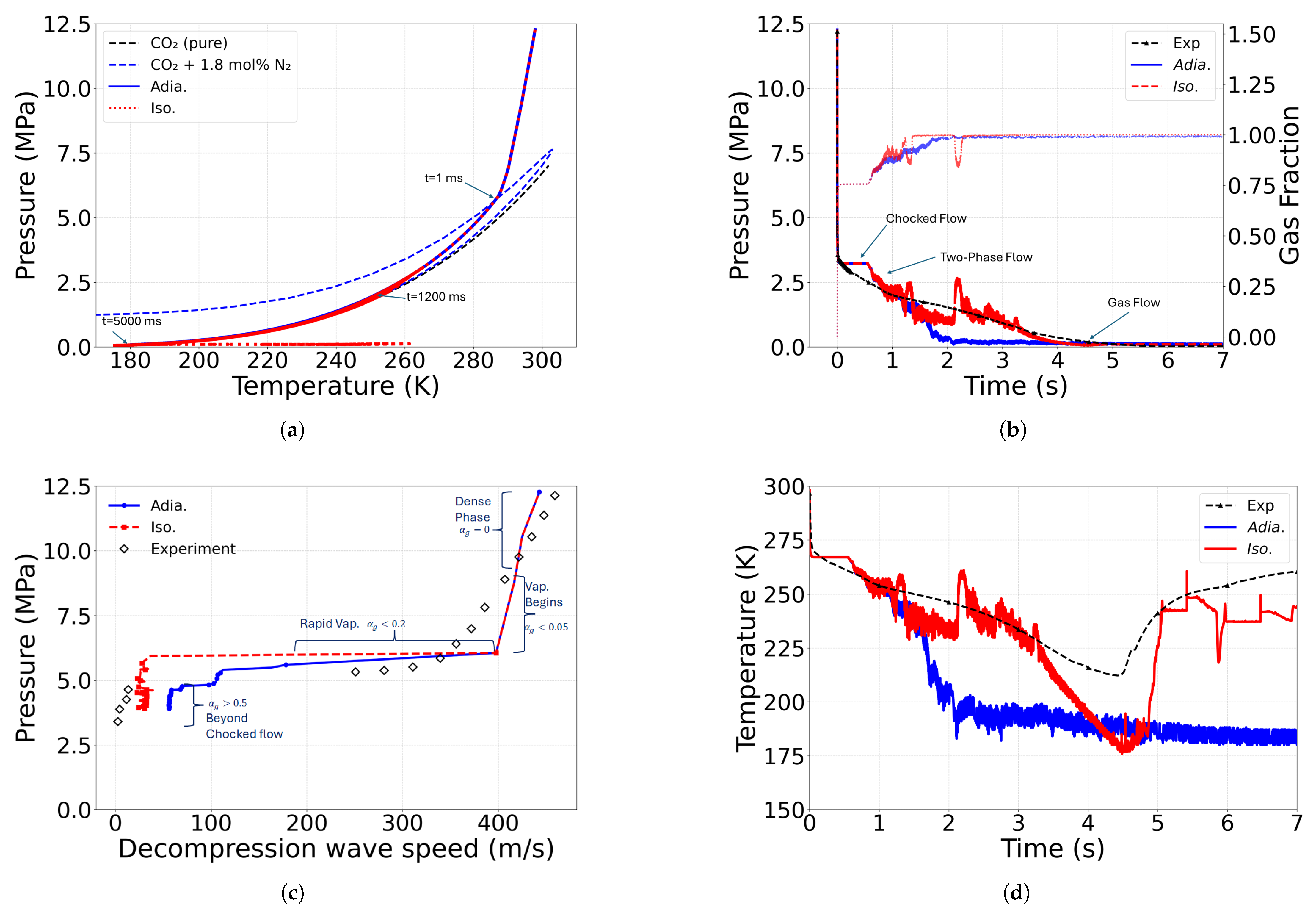
Previous studies (e.g., that by Mahgerefteh et al. [12] and subsequent works) have demonstrated that wall heat transfer and frictional effects can significantly alter decompression wave propagation. According to [12,64], for gas-like-phase sCO₂ shock-tube and convergent-divergent nozzle simulations, fluid–wall heat transfer and friction effects may be ignored for most short-duration decompression processes. However, the role of heat transfer in sCO₂ liquid-like pipeline depressurization has been widely recognized as a critical factor influencing the minimum temperature ($T_{min}$) reached during the depressurization by the two-phase fluid at the dew point. From a pipeline integrity point of view, it is well known that depressurization of CO₂ can lead to a very low $T_{min}$ within the pipeline. Performing depressurization too fast, the CO₂ might even reach the triple point (5.2 bar, −56.6 °C), resulting in the formation of dry ice and subsequent blockage of the stream, making the steel walls become brittle [89]. The present section presents a preliminary study of heat transfer and boundary conditions. It presents a qualitative trend of their effects on the cooling path and the minimum temperature ($T_{min}$) that could be attained by the system. Two boundary conditions, i.e., adiabatic and isothermal conditions, at the wall are compared. For the isothermal condition, the wall is assumed to be at the initial temperature, i.e., $T_{wall}=T_0=298$ K, throughout the observational time, i.e., 7 s. The isothermal wall assumption is a simplification compared to realistic pipeline conditions. However, the present study is on near-outlet decompression behavior, with analysis performed within 80 mm of the outlet. In this region, the transient flow and phase-change dynamics dominate over wall heat-transfer effects, particularly for short, laboratory-scale pipelines (60 m), making the assumption reasonable for the present scope. In Figure 3a,b,d, the system is found to follow the same thermodynamic path, pressure, and temperature profile in the initial phase (up to $1.5$ s), where the flow features are dominated by the initial shock-wave expansion, phase change, and Joule–Thompson cooling effect. Later on, for the two-phase state fluid and especially when the fluid becomes gaseous, the heat-transfer model starts showing major differences, as depicted in Figure 3a,c. It can be seen that a simplistic model of heat transfer that maintains the isothermal condition brings the depressurization pressure (Figure 3b) and temperature (Figure 3c) profiles close to the experimental data. Under the adiabatic condition, there is no source of heat intake into the fluid; hence, the fluid pressure rapidly decays to atmospheric pressure and stays at the minimum temperature obtained through Joule–Thompson cooling. Although the isothermal boundary condition is a better choice than an adiabatic wall, this study shows that wall heat transfer needs to be computed accurately to capture the transition of the decompression wave speed, as shown in Figure 3c for the various phases and the minimum temperature ($T_{min}$) attained by the system, as shown in Figure 3d. The isothermal condition is found to closely follow the behavior of the experimental data. In particular, the point at which the fluid transitions to the gaseous state and reaches $T_{min}$ agrees very well with the experimental results. Hence, although $T_{min}$ is underestimated when compared to available experiments, the isothermal wall is the chosen boundary condition for further study in this work.

These observations are consistent with previous studies on CO₂ pipeline decompression, where heat transfer and wall interactions have been shown to significantly influence pressure evolution and minimum temperature ($T_{min}$) prediction, particularly at longer time scales. While the isothermal assumption provides a reasonable approximation for short-duration decompression, more advanced approaches such as conjugate heat-transfer modeling are required for accurate long-term predictions and future work.

4.2. Effect of Equation of State

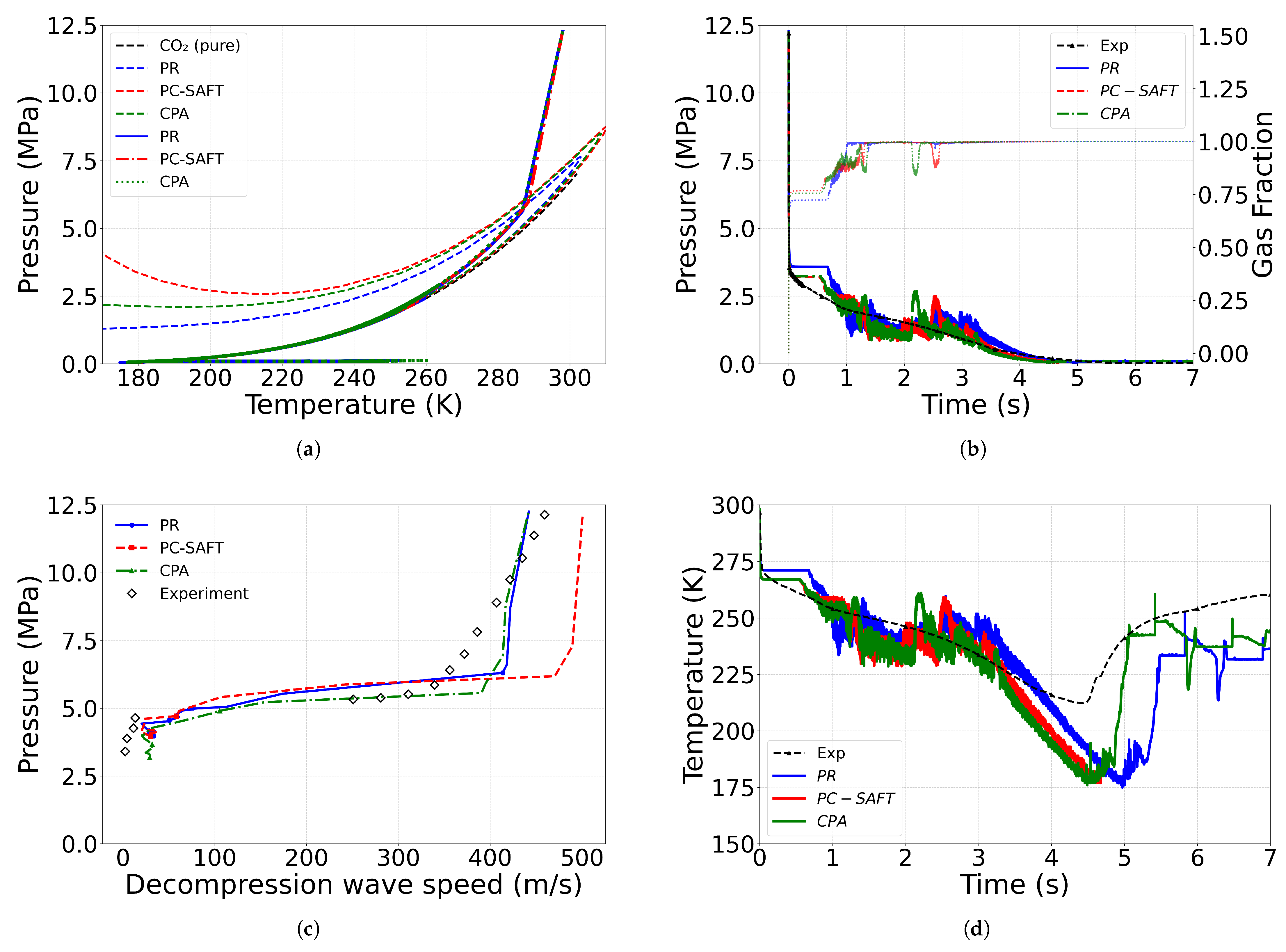
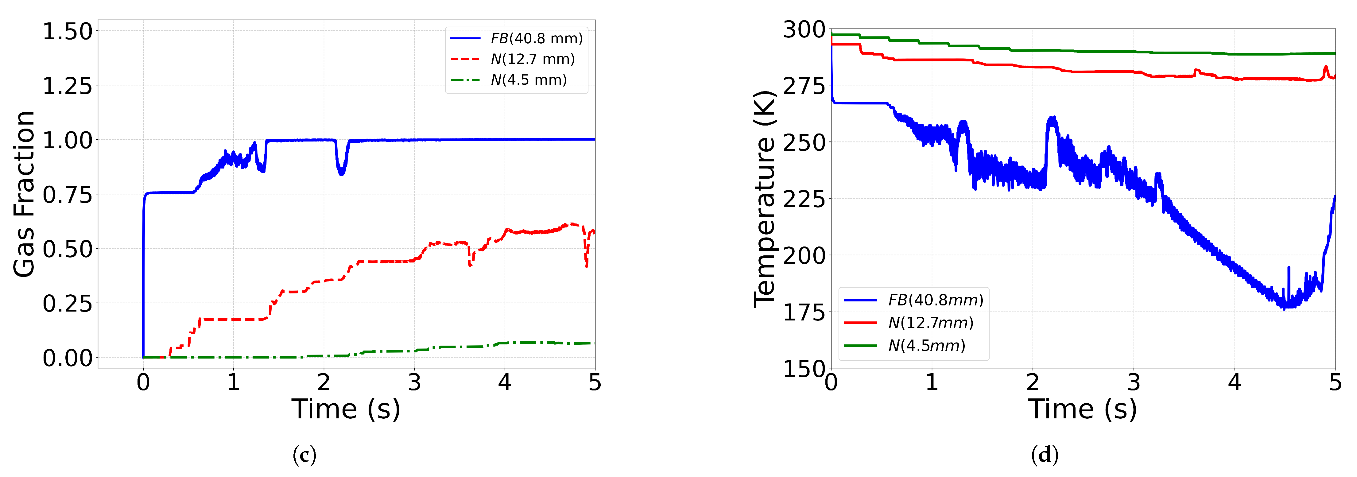
In contrast to conventional EoS assessments that focus primarily on equilibrium thermodynamic properties or vapor–liquid equilibrium prediction, the present analysis evaluates the influence of EoS selection (among available EoSs in our in-house CARNOT library [76]) on transient decompression dynamics within a CFD framework. The comparison presented here aims to assess EoS performance from both thermodynamic and flow-dynamics perspectives. It also aims to provide further justification for the conclusions set out earlier in the Introduction. Cases C1–C3 in Table 1 are investigated to assess the effect of the EoS on the depressurization behavior of sCO₂. Three widely used EoSs—namely, the CPA, Peng–Robinson (PR), and PC-SAFT EoSs—are considered in this study. These EoSs yield slight variations in the prediction of density, speed of sound, and phase equilibrium under near-critical and two-phase conditions. As a result, they influence key flow characteristics during depressurization, including pressure-wave propagation, the mass discharge rate, temperature evolution, and the onset and extent of phase change. The shape of the phase envelopes as computed from the three equations is shown in Figure 4. CPA and PC-SAFT show a higher critical temperature and pressure for the case of CO₂+N₂(1.8mol%). This also shifts the initiation point of vaporization at the bubble line (Figure 4a), resulting an order of saturation pressure of $Psa{t}_{PR}<Psa{t}_{CPA}<Psa{t}_{PC-SAFT}$ at a given temperature, while for the saturation temperature, the order is $Tsa{t}_{PR}>Tsa{t}_{CPA}>Tsa{t}_{PC-SAFT}$ at a given pressure. Because of differences in the bubble lines of the EoSs, the flow enters the two-phase flow state somewhat later for PR in comparison to CPA and PC-SAFT (see Figure 4a). Hence, a delayed chocked flow pressure and duration are observed for PR in comparison to CPA and PC-SAFT, as can be seen at about 1 s in the pressure and temperature evolution plotted in Figure 4b,d. For the current monitor point, the flow enters the gaseous phase at the dew point at about $4.5$ s after two interactions with reflected pressure waves from the closed end of the pipe, which lead to more or fewer pressure oscillations in the two-phase flow region. The depressurization rate is different at each stage of interaction, and so is the gas fraction. It should be noted that, in Figure 4a, the pressure curve remains tangent to the dew line for a considerable time. This period of low liquid fraction, lasting approximately 2.5 s, is characterized by sharp drops in both pressure and, in particular, temperature, as shown in Figure 4d. The flow leaves the phase envelope or enters the gaseous state at an almost identical thermodynamic state for all EoSs. Figure 4c shows a comparison of the decompression wave speed ($u_w$) for various EoSs, as it is highly dependent on speed of sound predicted by the EoS for a given phase and needed for ductile fracture studies, for instance. It is observed that the CPA model predicts the decompression wave speed and the transition pressure well, while the PC-SAFT model overpredicts the decompression wave speed and the PR model overpredicts the transition pressure. Although these results are in line with previous studies, the current investigations highlight that the suitability of an equation of state in decompression modeling cannot be assessed solely based on equilibrium thermodynamic accuracy. Instead, its ability to consistently predict flow-coupled quantities such as decompression wave speed and transition pressure becomes equally important. In this regard, the CPA model demonstrates improved predictive capability for the present application, justifying its selection for subsequent analyses.

4.3. Effect of Impurity

4.3.1. Comparison with Pure CO₂

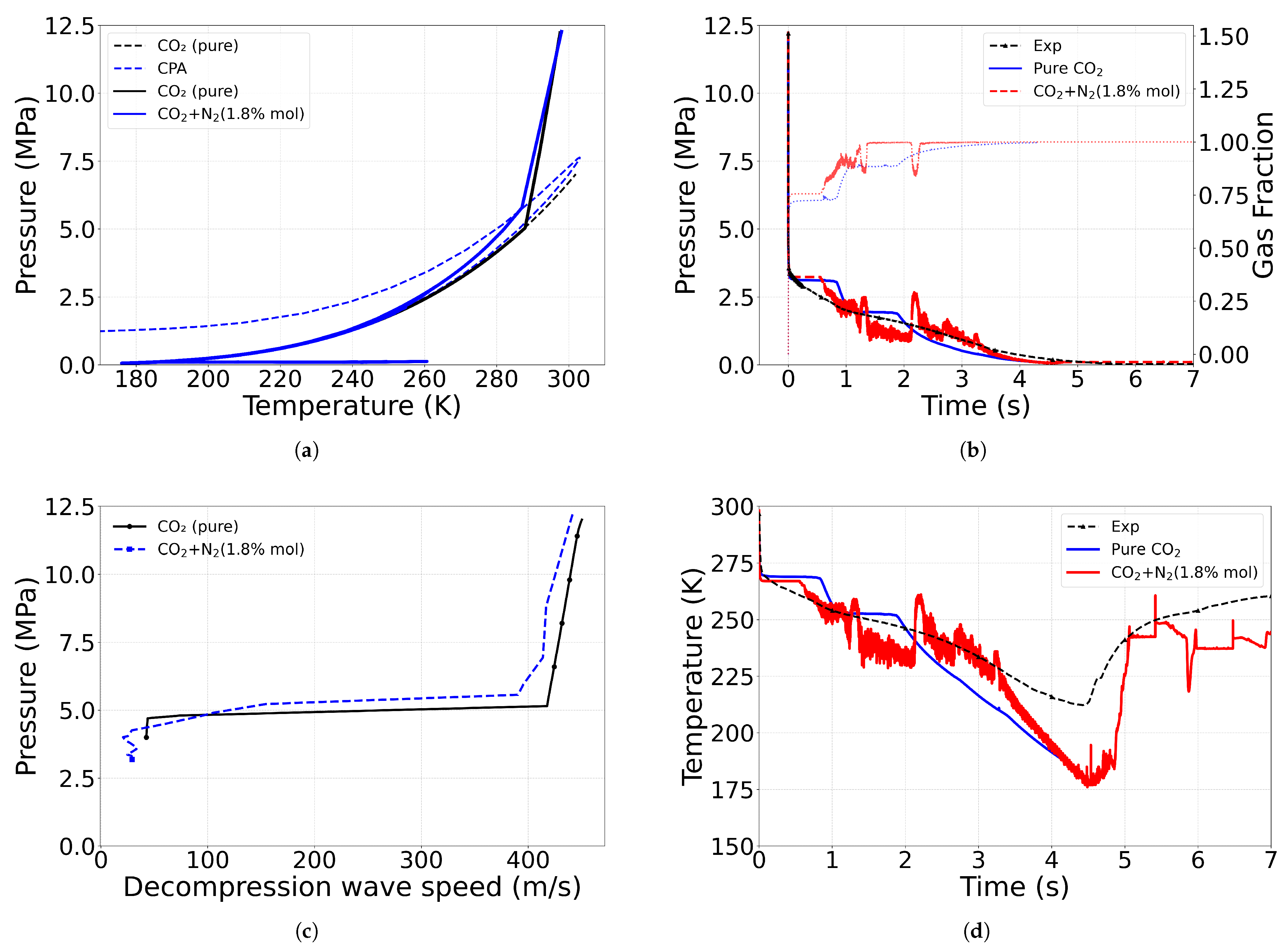
This section compares cases of pure CO₂ and the CO₂+N₂(1.8mol%) mixture, i.e., cases C0 and C1 in Table 2. It should be noted that a PH-Flash algorithm is used in the IFPEN-Carnot library [76] to determine the phase-transition and equilibrium properties of pure CO₂. The CPA EoS is used for the generation of an appropriate table of thermodynamic and transport properties, as discussed in Section 2.2. Figure 5 shows a comparison of the thermodynamic state, pressure, and gas volume fraction profiles, as well as the decompression wave speed for pure and rich CO₂ mixtures. The saturation point at which vaporization starts is well predicted for both pure CO₂ and the CO₂+N₂(1.8% mol) mixture. As shown in Figure 5a, the depressurization rate is slightly higher for pure CO₂ in comparison to CO₂ with impurities, as the steepness and the saturation point are lower for pure CO₂. The gas volume fraction at a chocked flow state is also higher for pure CO₂ in comparison to rich CO₂ mixtures (Figure 5b). In the Figure, two reflected pressure waves from the pipeline’s closed end can be clearly seen, without spurious oscillations induced by the impurity for the rich CO₂ mixture. In addition, the transition pressure for the decompression wave speed ($u_w$) for pure CO₂ is lower than with impurities, as also depicted from the phase envelope. The thermodynamic state of entering the gaseous state is close for pure and rich CO₂ mixtures. However, the period with a low liquid fraction (where the saturation line is tangent to the dew line; Figure 5a), lasting approximately 2.5 s, is characterized by a sharp drop in temperature, as shown in Figure 5d. Finally, one may note that the present simulation predicts a steeper temperature slope, in addition to a larger chocked flow state, in comparison to the experiments [31,77], which must be further investigated in future work.

4.3.2. Comparison Between Different Impurities (N₂, CH₄, and Ar)

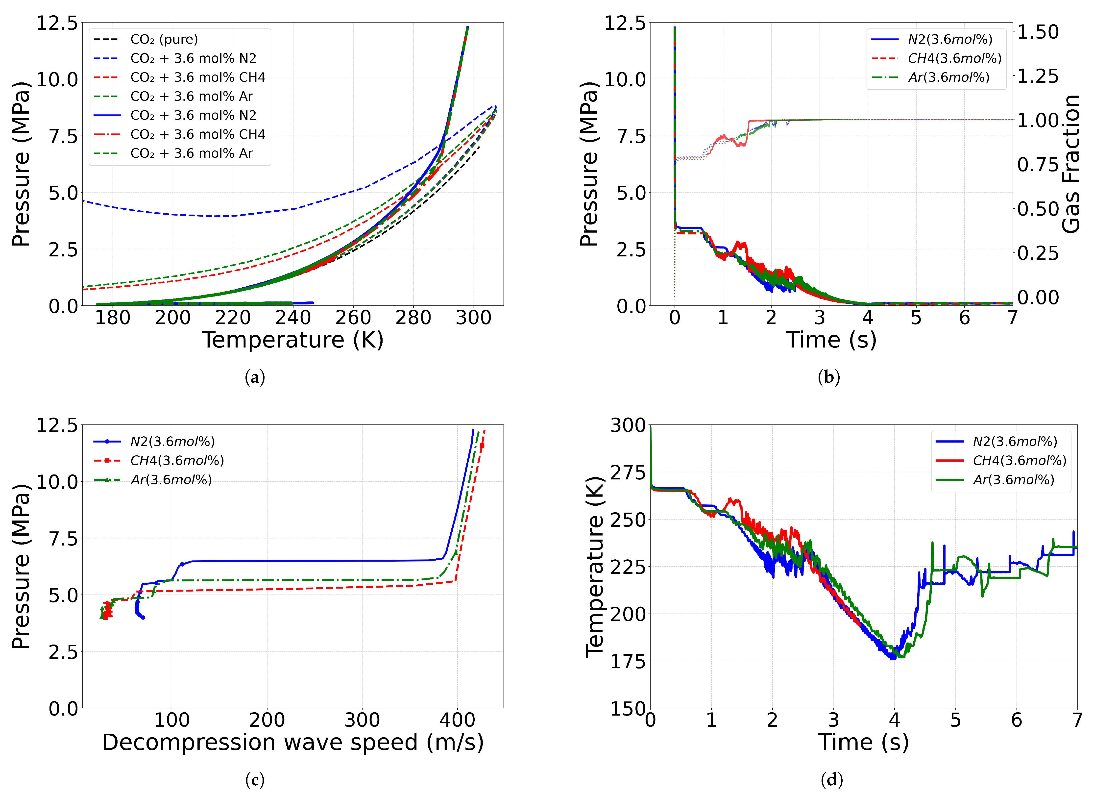
As discussed in the Introduction (Section 1), the selected binary systems are CO₂-N₂, CO₂-CH₄, and CO₂-Ar, representing the major non-condensable impurities relevant to current and emerging sCO₂ capture, transport, and storage applications [79]. The depressurization behavior of multi-component fluids is governed by a combination of thermodynamic, caloric, and transport properties, including the mixture’s molar mass, critical properties, acentric factor, phase-equilibrium characteristics, speed of sound, Joule–Thomson coefficient, and heat capacity. Figure 6 shows a comparison of the thermodynamic state, pressure, gas fraction, and decompression wave speed for Cases C4, C6, and C8. Since the speed of sound ($C_s$) and the critical compressibility factor ($Z_c$) are close to each other for all the mixtures under the given initial condition, which is very close to critical point for supercritical flows, the depressurization rate and the pressure profile are also close to each other until vaporization begins, as shown in Figure 6a. Indeed, the point of vaporization obviously differs for each case, but the thermodynamic state paths inside the phase envelope collapse again before the dew point and the gaseous phase, as also shown in Figure 6a. The transition pressure of the decompression wave speed decreases in the same order (N₂ > Ar > CH₄); then, the saturation plateaus in Figure 6c. Similarly, the decompression wave speed for the gaseous (or liquid) phase in Figure 6c also increases (or decreases) in the same order, i.e., N₂ > Ar > CH₄. Finally, changing the impurity does not induce significantly different results near the critical point during depressurization, although few differences occur in the pressure and temperature evolutions, mainly during the two-phase stage, as shown in Figure 6b,d.

4.3.3. Role of Impurity Mass Fraction

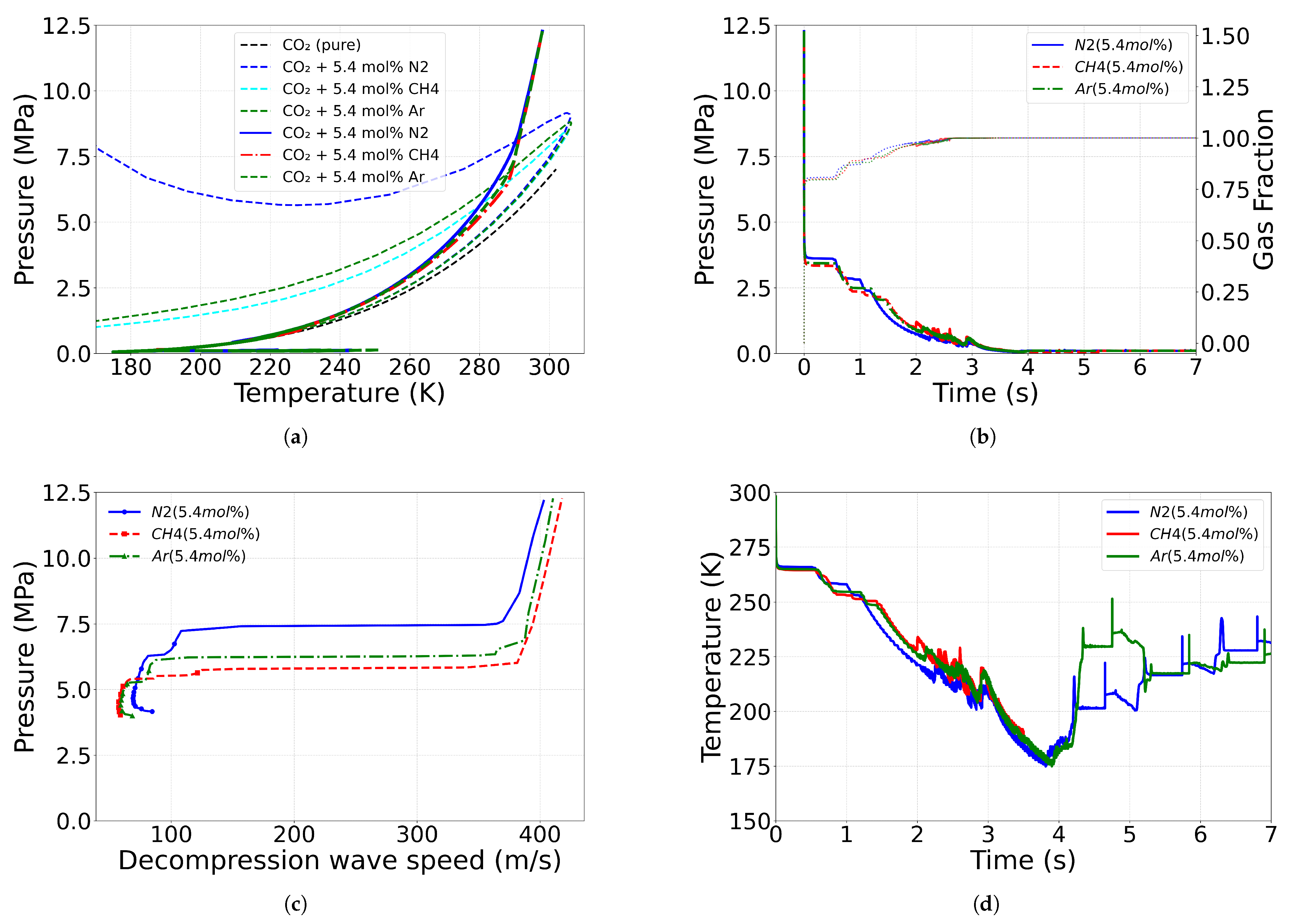
Comparison of Figure 6 and Figure 7 shows the effect of the mole fraction on the depressurization thermodynamic path, pressure, gas volume fraction, and decompression wave speed. The increase in mole fraction of impurities shifts the phase envelope upwards, accordingly shifting the onset pressure of vaporization, chocked flow pressure, and gas fraction. As shown in Figure 6c and Figure 7c, for low-composition mixtures, the decompression wave speed in the dense phase at $t=0$ is closer to pure CO₂ and remains the same for all the mixtures, i.e., 410 m/s. However, for higher impurity concentrations, the effect of impurities on the wave speed becomes visible. The decompression wave speed for dense phases decreases in the following order: CH₄ (427 m/s) > Ar (410 m/s) > N₂ (400 m/s). It should be noted that the minimum temperature ($T_{min}$) reaches very similar values, of the order of 175 K, regardless of the amount of impurities, as shown in Figure 6d and Figure 7d.

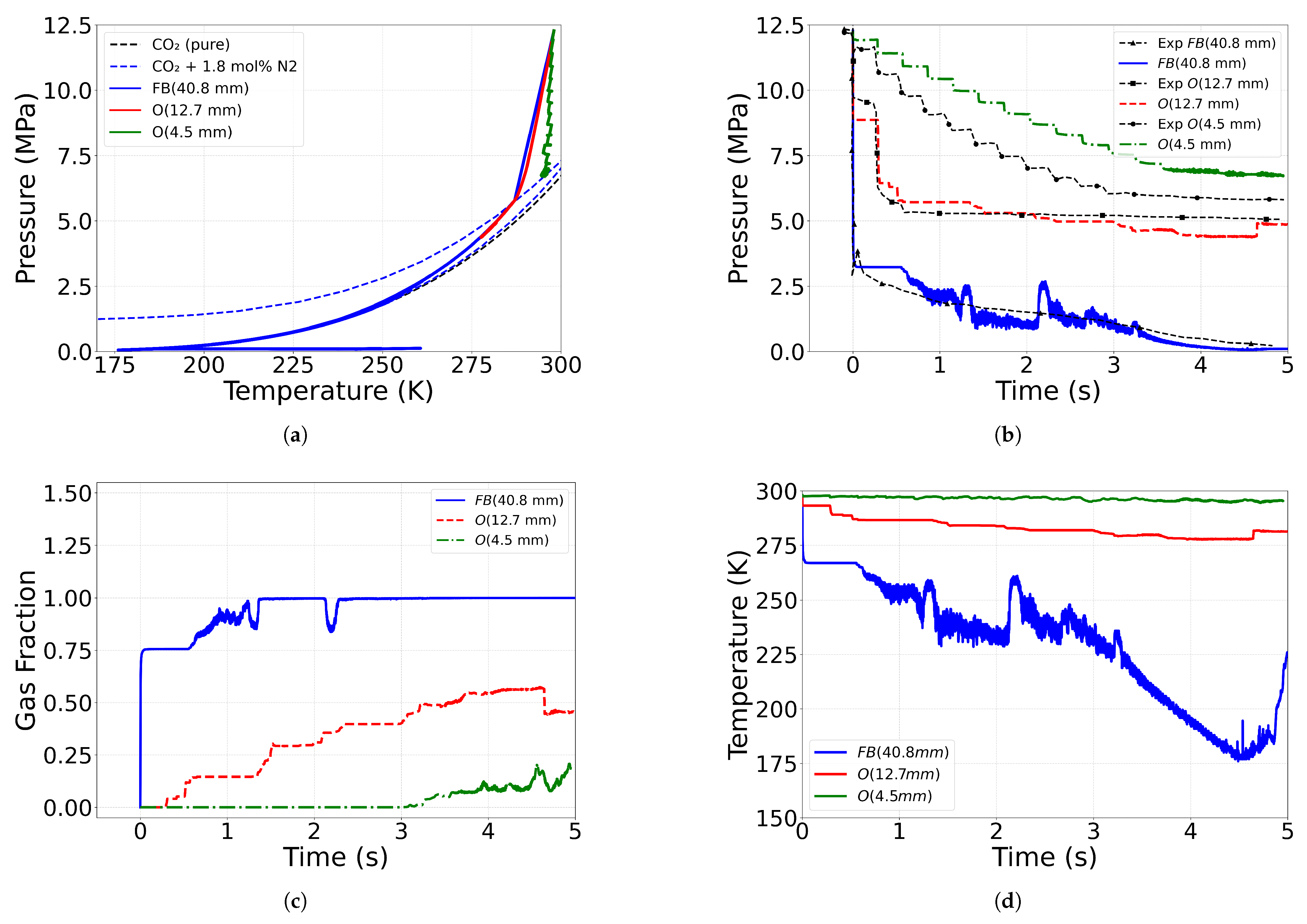
4.4. Effects of Outlet Geometry and Diameter

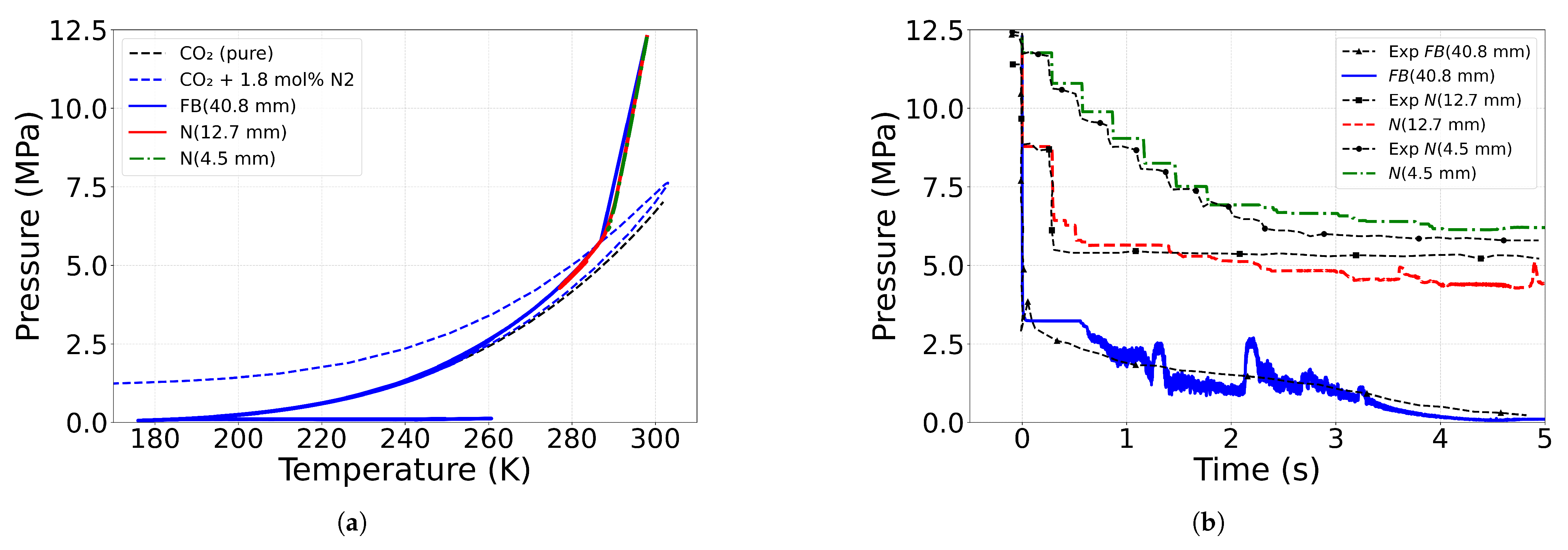
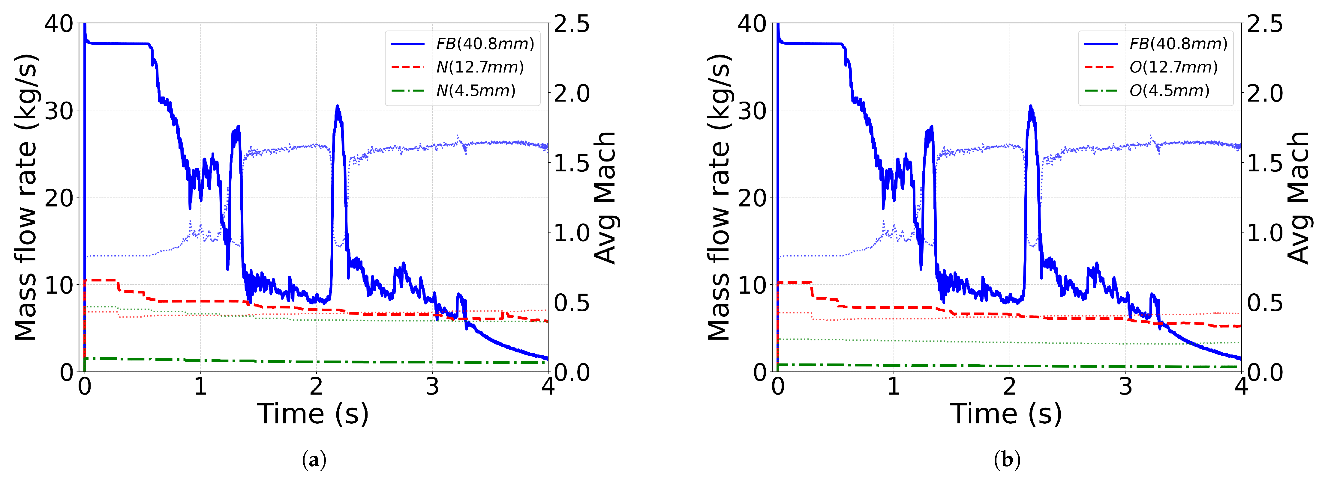
Cases C10–C13 in Table 3 analyze the effects of outlet geometry and diameter. For the case of the orifice, a rectangular outlet boundary is used as an area-equivalent representation of the circular geometry, ensuring that the effective discharge area remains identical, as depicted in Figure 1b. In our preliminary studies), it was found that such a variation in boundary geometry does not alter the pressure, gas volume fraction, or temperature traces. Thus, such a simplification is used because it improves the grid quality and facilitates mesh generation while preserving the dominant flow characteristics, since the choked mass flow rate is primarily governed by the minimum flow area and upstream thermodynamic state [78]. However, it is acknowledged that local geometric effects such as vena-contracta formation and discharge coefficient variations are inherently geometry-dependent and may not be fully captured by this representation. The results presented in this section follow a trend similar to that reported in the experimental work of Hammer et al. [78]. However, a slight difference in the chocked flow state is expected, as the present simulation in conducted with N₂ (1.8% by mol) as an impurity. Figure 8 and Figure 9 illustrate that variations in outlet geometry and diameter modify the discharge characteristics, with smoother geometries (e.g., nozzle) promoting gradual flow acceleration, while abrupt contractions (e.g., orifice) introduce additional localized losses due to rapid area change; however, as vaporization, begins the system follows a similar thermodynamic path. The resulting reduction in effective discharge capacity leads to a lower mass flow rate and, consequently, a slower depressurization rate, as reflected in the pressure profile. Therefore, the thermodynamic path tends to shift rightward, representing higher density for a reduced mass flow rate. It is noted that the present quasi-one-dimensional discretization captures the overall influence of outlet geometry through global flow quantities (see the excellent results when compared to the nozzle experiments in Figure 8b). However, localized three-dimensional effects such as separation and recirculation near sharp geometrical transitions are not explicitly resolved and may contribute to additional losses, particularly in orifice configurations (see the less accurate results when compared to the orifice experiments (4.5 mm) from the outlet in Figure 9b). The decompression wave speed does not have a clear demarcation for the dense phase and gaseous phase for these cases, as the fluid remains in the two-phase state for the simulated time. Also, a prolonged chocked flow state brings about difficulty in estimating the instantaneous time for a given pressure level and, consequently, difficulty in calculating an accurate decompression wave speed. Hence, the decompression wave-speed plot is omitted for the present section. It is also noteworthy that the simulations become numerically more unstable under choked flow conditions, therefore requiring a smaller time step $\left(dt\right)$ to maintain stability.

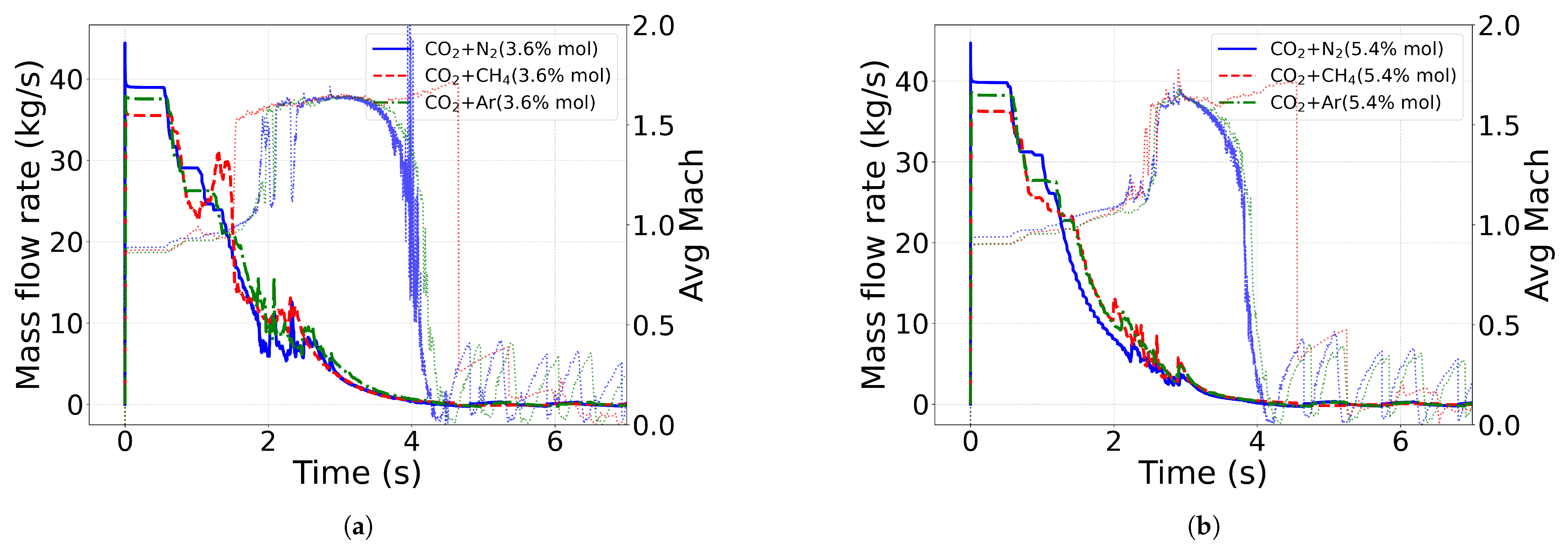
4.5. Mass Flow Rate and Mach Number

The primary objective of this work is to develop a database of the mass flow rate, pressure, and gas-phase properties that can serve as inputs for dispersion models predicting the spread of CO₂ mixtures during pressure leakage events. In current industrial practice, discharge predictions largely rely on steady or quasi-steady formulations and empirical choked-flow correlations. These approaches depend strongly on the mixture speed of sound and its variation during phase change. Therefore, the present study reports both the mass flow rate and Mach number for comparison. All reported quantities in Figure 10 correspond to mass-averaged values evaluated on the rupture/outflow plane. Density and velocity are coupled with one another, with variation always in both to maintain continuity. Initially, the density is higher, representing the presence of liquid, then reducing to air density. Accordingly, the velocity varies, and variations in pressure and temperature in previous plots and the mass fraction in Figure 10 and Figure 11 represent the sudden change in gas fraction caused during two instances of the simulation: when released from the chocked flow state and when phase changes from two-phase to the gas phase. The initial chocked flow condition is the duration of the fluid exiting at the maximum mass flow rate. This maximum mass flow rate for each impurity is found to be less dependent on the mixture composition (i.e., mol % 3.6–5.4) and mostly a function of the initial (supercritical) and outflow conditions only. However, when comparing the different impurities, the maximum mass flow rate decreases in the order of N₂ > Ar > CH₄. The flow enters the two-phase state under subsonic conditions but close to Mach 1 (i.e., $M_{en}\simeq 0.8$), while close to the gaseous state, the fluid Mach number rises rapidly to balance the decrease in density and maintain continuity. The maximum Mach number is found to be close to 1.7 (i.e., $M_{out}\simeq 1.7$) and is attained in the two-phase region before transitioning to the gaseous phase, where the Mach number decreases abruptly due to the higher speed of sound in the gaseous state. Similarly, Figure 11 reports the mass flow rate and Mach number for various outlet diameters and geometries in the present study. The mass flow rate for the nozzle is found to be closer to the experimental data but not for the orifice. This could be because of the sharp change in the flow field for the case of the orifice in comparison to the nozzle. The effect of vena-contracta and the coefficient of discharge is severe for the case of the orifice and needs to be considered and modeled more accurately.

5. sCO₂ Pipeline Transport: Industrial-Scale Simulation

For real-life applications, pipeline transport expands to the order of km instead of m. For such a configuration, a 50 km long pipeline depressurization case was studied in [89]. A simulation of this scale generates increased complexity, particularly in terms of computational costs. A wall heat-transfer model, pressure loss along the pipeline, venting tubes, turbulence, and gravity effects cannot be neglected anymore. The present study is intended as a exploratory analysis to assess the influence of decompression physics under simplified conditions and analyze the modeling capabilities of the RFM framework recently implemented by IFPEN in the CONVERGE solver. Factors such as wall friction, roughness, and terrain-induced elevation changes are important for long-distance pipeline simulations and will be addressed in future works.

5.1. Setup of the 50 km Pipeline with Venting

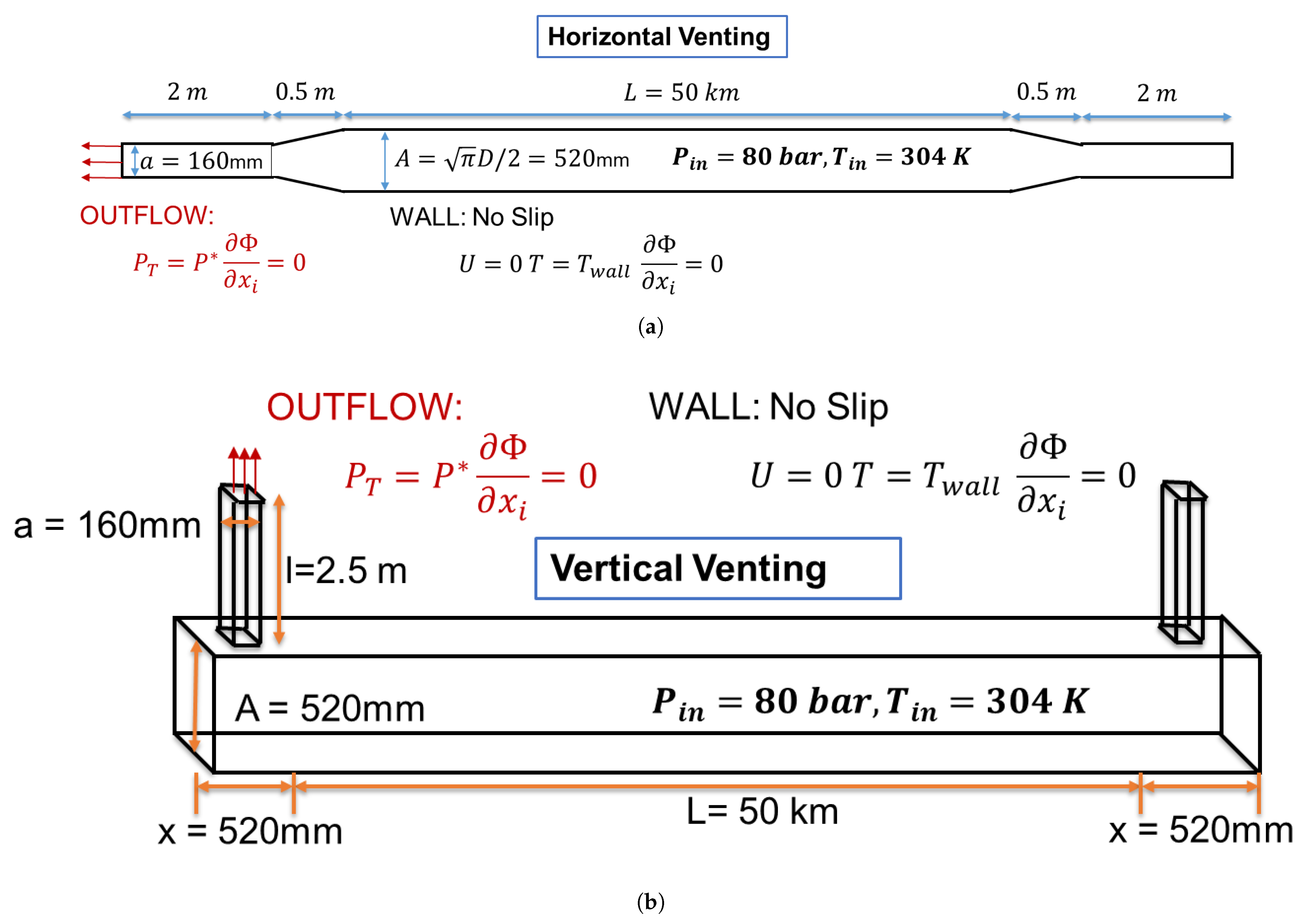
A rectangular geometry is chosen instead of a circular cylinder for simplicity for the case of 50 km long pipe depressurization, keeping the effective area identical to that of an actual circular pipeline. In a few preliminary simulations, it is observed that the venting configuration plays a significant role in the depressurization dynamics, as the venting pipe’s diameter ($d=7\mathrm{inch}$) is substantially smaller than the main pipeline’s diameter ($d=24\mathrm{inch}$). This pronounced area contraction governs the discharge characteristics and strongly influences the pressure decay rate. Therefore, two different venting configurations, i.e., horizontal and vertical venting, are investigated taking advantage of the 3D-based finite volume method used in this work. Detailed descriptions of both configurations are shown in Figure 12. The boundary conditions are similar to the previous short pipeline setup, i.e., Dirichlet for pressure at the outlet, isothermal for the wall, and no slip condition along the rest of the wall. Boundary conditions, along with initial conditions, are also shown in Figure 12.

5.2. Pressure and Temperature Profiles

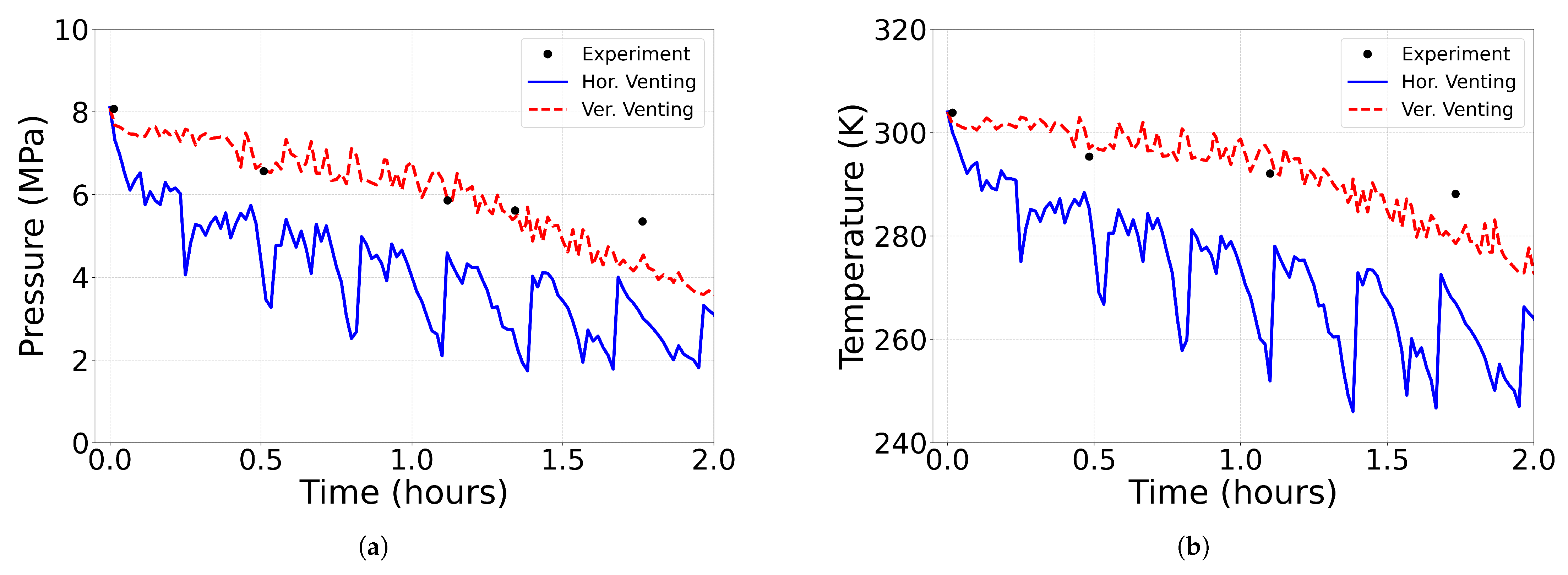
It can be seen from Figure 13a,b that the vertical venting configuration outperforms the horizontal one to a great extent, implying not only that the venting area is important but also the role of gravity for such a configuration. The pressure profiles tend to follow a trend similar to the experimental results for both the configurations, with vertical venting being closer to the experimental data. Some deviations begin when the simulation is close to 2 h in the physical time scale, as the effects of heat transfer and pipe loss are expected to be predominant after such a long duration. Hence, future work will involve analysis of the problem with a coupled conjugate heat-transfer model, along with a skelitic pipeline configuration. The horizontal venting configuration requires approximately 2 days of wall-clock time on 256 cores to simulate 2 h of physical time. In contrast, the vertical venting configuration requires nearly 8 days with identical computational resources and simulation duration. The extended computational time is primarily due to the severe time-step restriction imposed by the physics of the problem. The allowable time step is limited by stability constraints, which are directly linked to the smallest cell volume in the domain. Larger time steps would require larger cell volumes; however, this is not feasible in the present case. In the vertical venting configuration, resolving gravity-driven stratification and slip effects in the venting section requires maintenance of a minimum of 10 cells along the vertical direction. This refinement significantly reduces the minimum cell volume in the domain, thereby imposing a much smaller stable time step and consequently increasing the total computational time.

6. Conclusions

The present work shows that the real-fluid model (RFM) equilibrium framework is capable of modeling supercritical CO₂ pipeline transport problems with good accuracy. A good match was found between simulation results and experimental data, although different simplifying assumptions were employed. First, the isothermal heat-transfer model and the CPA EoS were proven to be most suitable for sCO₂ fluid simulations. Next, the role of impurities was investigated. Although impurities not only shift thermodynamic boundaries but also alter the kinetics of phase transitions, it was revealed that the amount of impurities is less predominant near critical-condition operations, as the depressurization rate, wave speed, and pressure profiles were found to be similar. The outlet geometry also tends to impact the thermodynamic path to a great extent. It was found that for nozzle geometries where there is a smooth change in the cross-section area, the simulation predictions were in excellent agreement with the experimental data. However, for the case of orifices where there is a sharp change in the cross-section area, the simulation underpredicts the leakage mass flow rate, implying a necessary computationally refined discretization for the outlet geometry. Finally, the role of the venting area was found to be predominant for the 50 km sCO₂ pipeline depressurization to capture the initial physics of depressurization. The conjugate heat-transfer (CHT) model and modeling of losses in pipes at the wall level become essential for subsequent stages when considering buried pipelines. Therefore, the present industrial-scale analysis should be interpreted as an exploratory demonstration, with future work directed toward the incorporation of conjugate heat transfer and more detailed pipeline representations for enhanced predictive capability.

References

1. Eide, L.I.; Batum, M.; Dixon, T.; Elamin, Z.; Graue, A.; Hagen, S.; Hovorka, S.; Nazarian, B.; Nøkleby, P.H.; Olsen, G.I.; et al. Enabling large-scale carbon capture, utilisation, and storage (CCUS) using offshore carbon dioxide (CO2) infrastructure developments—A review. Energies 2019, 12, 1945. [Google Scholar] [CrossRef]
2. Rui, Z.; Zeng, L.; Dindoruk, B. Challenges in the large-scale deployment of CCUS. Engineering 2025, 44, 17–20. [Google Scholar] [CrossRef]
3. Boot-Handford, M.E.; Abanades, J.C.; Anthony, E.J.; Blunt, M.J.; Brandani, S.; Mac Dowell, N.; Fernández, J.R.; Ferrari, M.C.; Gross, R.; Hallett, J.P.; et al. Carbon capture and storage update. Energy Environ. Sci. 2014, 7, 130–189. [Google Scholar] [CrossRef]
4. Leung, D.Y.; Caramanna, G.; Maroto-Valer, M.M. An overview of current status of carbon dioxide capture and storage technologies. Renew. Sustain. Energy Rev. 2014, 39, 426–443. [Google Scholar] [CrossRef]
5. Haszeldine, R.S. Carbon capture and storage: How green can black be? Science 2009, 325, 1647–1652. [Google Scholar] [CrossRef]
6. Wareing, C.J.; Fairweather, M.; Falle, S.A.; Woolley, R.M. Modelling ruptures of buried high pressure dense phase CO2 pipelines in carbon capture and storage applications—Part I. Validation. Int. J. Greenh. Gas Control 2015, 42, 701–711. [Google Scholar] [CrossRef]
7. Martynov, S.; Zheng, W.; Mahgerefteh, H.; Brown, S.; Hebrard, J.; Jamois, D.; Proust, C. Computational and experimental study of solid-phase formation during the decompression of high-pressure CO2 pipelines. Ind. Eng. Chem. Res. 2018, 57, 7054–7063. [Google Scholar] [CrossRef]
8. Brown, S.; Martynov, S.; Mahgerefteh, H.; Chen, S.; Zhang, Y. Modelling the non-equilibrium two-phase flow during depressurisation of CO2 pipelines. Int. J. Greenh. Gas Control 2014, 30, 9–18. [Google Scholar] [CrossRef]
9. Peletiri, S.P.; Rahmanian, N.; Mujtaba, I.M. CO2 Pipeline design: A review. Energies 2018, 11, 2184. [Google Scholar] [CrossRef]
10. Bielka, P.; Kuczyński, S.; Włodek, T.; Nagy, S. Risks and safety of CO2 pipeline transport: A case study of the analysis and modeling of the risk of accidental release of CO2 into the atmosphere. Energies 2024, 17, 3943. [Google Scholar] [CrossRef]
11. Lu, H.; Ma, X.; Huang, K.; Fu, L.; Azimi, M. Carbon dioxide transport via pipelines: A systematic review. J. Clean. Prod. 2020, 266, 121994. [Google Scholar] [CrossRef]
12. Mahgerefteh, H.; Brown, S.; Martynov, S. A study of the effects of friction, heat transfer, and stream impurities on the decompression behavior in CO2 pipelines. Greenh. Gases Sci. Technol. 2012, 2, 369–379. [Google Scholar] [CrossRef]
13. Woolley, R.M.; Fairweather, M.; Wareing, C.J.; Falle, S.A.; Mahgerefteh, H.; Martynov, S.; Brown, S.; Narasimhamurthy, V.D.; Storvik, I.E.; Saelen, L.; et al. CO2PipeHaz: Quantitative hazard assessment for next generation CO2 pipelines. Energy Procedia 2014, 63, 2510–2529. [Google Scholar] [CrossRef]
14. Wareing, C.J.; Fairweather, M.; Woolley, R.M.; Falle, S.A. Numerical simulation of CO2 dispersion from punctures and ruptures of buried high-pressure dense phase CO2 pipelines with experimental validation. Energy Procedia 2014, 63, 2500–2509. [Google Scholar] [CrossRef]
15. Pham, L.H.H.P.; Rusli, R. A review of experimental and modelling methods for accidental release behaviour of high-pressurised CO2 pipelines at atmospheric environment. Process Saf. Environ. Prot. 2016, 104, 48–84. [Google Scholar] [CrossRef]
16. Munkejord, S.T.; Hammer, M.; Løvseth, S.W. CO2 transport: Data and models–A review. Appl. Energy 2016, 169, 499–523. [Google Scholar] [CrossRef]
17. Vitali, M.; Corvaro, F.; Marchetti, B.; Terenzi, A. Thermodynamic challenges for CO2 pipelines design: A critical review on the effects of impurities, water content, and low temperature. Int. J. Greenh. Gas Control 2022, 114, 103605. [Google Scholar] [CrossRef]
18. Shang, Y.; Chen, X.; Yang, M.; Xing, X.; Jiao, J.; An, G.; Li, X.; Xiong, X. Comprehensive review on leakage characteristics and diffusion laws of carbon dioxide pipelines. Energy Fuels 2024, 38, 10456–10493. [Google Scholar] [CrossRef]
19. Gu, S.; Li, Y.; Teng, L.; Hu, Q.; Zhang, D.; Ye, X.; Wang, C.; Wang, J.; Iglauer, S. A new model for predicting the decompression behavior of CO2 mixtures in various phases. Process Saf. Environ. Prot. 2018, 120, 237–247. [Google Scholar] [CrossRef]
20. Magen, O.; Kozak, Y.; Di Lucchio, L.; Marengo, M.; Bar-Kohany, T. Predicting nucleation pressure under rapid depressurization: Bridging positive and negative pressure regions. Int. J. Heat Mass Transf. 2025, 251, 127309. [Google Scholar] [CrossRef]
21. He, X.; Gao, P.; Wang, J.; Zhang, Z. Experimental investigation on hot water rapid depressurization process characteristics inside and outside of the ruptured pipeline. Nucl. Eng. Des. 2024, 425, 113341. [Google Scholar] [CrossRef]
22. Liao, H.; Wang, X.; Yang, K.; Hou, Z.; Wang, H. Impurity-driven variations in CO2 critical flow dynamics: Modeling approaches for enhanced CCS safety. Energy 2025, 323, 135850. [Google Scholar] [CrossRef]
23. Cao, Q.; Yan, X.; Liu, S.; Yu, J.; Chen, S.; Zhang, Y. Temperature and phase evolution and density distribution in cross section and sound evolution during the release of dense CO2 from a large-scale pipeline. Int. J. Greenh. Gas Control 2020, 96, 103011. [Google Scholar] [CrossRef]
24. Hansen, P.M.; Gaathaug, A.V.; Bjerketvedt, D.; Vaagsaether, K. The behavior of pressurized liquefied CO2 in a vertical tube after venting through the top. Int. J. Heat Mass Transf. 2017, 108, 2011–2020. [Google Scholar] [CrossRef]
25. Hansen, P.M.; Gaathaug, A.V.; Bjerketvedt, D.; Vaagsaether, K. Rapid depressurization and phase transition of CO2 in vertical ducts–small-scale experiments and Rankine-Hugoniot analyses. J. Hazard. Mater. 2019, 365, 16–25. [Google Scholar] [CrossRef]
26. Bhuvankar, P.; Cihan, A.; Birkholzer, J. A framework to simulate the blowout of CO2 through wells in geologic carbon storage. Int. J. Greenh. Gas Control 2023, 127, 103921. [Google Scholar] [CrossRef]
27. Yin, B.; Huang, W.; Ouyang, X.; Zhao, X.; Meng, L.; Zhang, L.; Hu, Q.; Li, Y. A transient model considering non-equilibrium phase transition in CO2 pipe decompression. J. Pipeline Sci. Eng. 2025; in press.
28. Log, A.M.; Hammer, M.; Deng, H.; Austegard, A.; Hafner, A.; Munkejord, S.T. Depressurization of CO2 in a pipe: Effect of initial state on non-equilibrium two-phase flow. Int. J. Multiph. Flow 2024, 170, 104624. [Google Scholar] [CrossRef]
29. Wang, J.; Lu, Z.; Wu, S.; Zhang, Z.; Liu, J. Research on non-equilibrium characteristics and relaxation time parameter optimization in high-pressure CO2 pipeline depressurization. Int. Commun. Heat Mass Transf. 2025, 169, 109527. [Google Scholar] [CrossRef]
30. Log, A.M.; Hammer, M.; Munkejord, S.T. A flashing flow model for the rapid depressurization of CO2 in a pipe accounting for bubble nucleation and growth. Int. J. Multiph. Flow 2024, 171, 104666. [Google Scholar] [CrossRef]
31. Munkejord, S.T.; Deng, H.; Austegard, A.; Hammer, M.; Aasen, A.; Skarsvåg, H.L. Depressurization of CO2-N2 and CO2-He in a pipe: Experiments and modelling of pressure and temperature dynamics. Int. J. Greenh. Gas Control 2021, 109, 103361. [Google Scholar] [CrossRef]
32. Yu, S.; Yan, X.; He, Y.; Chen, L.; Hu, Y.; Yang, K.; Cao, Z.; Yu, J.; Chen, S. Study on the decompression behavior during large-scale pipeline puncture releases of CO2 with various N2 compositions: Experiments and mechanism analysis. Energy 2024, 296, 131180. [Google Scholar] [CrossRef]
33. Zhu, J.; Wu, J.; Xie, N.; Li, Z.; Hu, Q.; Li, Y. Study on water hammer phase transition characteristics of dense/liquid phase CO2 pipeline. Energy 2024, 311, 133470. [Google Scholar] [CrossRef]
34. Liao, H.; Yang, K.; Liang, Z.; Hu, H.; Wang, X.; Wang, H. A new paradigm in critical flow analysis: Combining Buckingham Pi theorem with neural network for improved predictions in microchannels. Chem. Eng. Sci. 2024, 299, 120483. [Google Scholar] [CrossRef]
35. Yu, S.; Yan, X.; He, Y.; Hu, Y.; Qiao, F.; Yang, K.; Cao, Z.; Chen, L.; Liu, Z.; Yu, J.; et al. Study on the effect of valve openings and multi-stage throttling structures on the pressure and temperature during CO2 pipeline venting processes. Energy 2024, 308, 132967. [Google Scholar] [CrossRef]
36. Ding, Y.; Xu, P.; Lu, Y.; Yang, M.; Zhang, J.; Liu, K. Research on pipeline leakage calculation and correction method based on numerical calculation method. Energies 2023, 16, 7255. [Google Scholar] [CrossRef]
37. Zhang, Z.; Lu, Z.; Yan, L.; Wang, J.; Yao, S. Experiment and numerical investigation on flow characteristics and near-field structure of dense phase CO2 pipeline leakage. Process Saf. Environ. Prot. 2024, 182, 327–344. [Google Scholar] [CrossRef]
38. Yu, S.; Yan, X.; He, Y.; Yu, J.; Chen, S. Study on the leakage morphology and temperature variations in the soil zone during large-scale buried CO2 pipeline leakage. Energy 2024, 288, 129674. [Google Scholar] [CrossRef]
39. Shang, Y.; Xing, X.; Chen, X.; Yang, M.; Shah, R.K.; Pang, X. Developing Transient Model and Simulating the Effects of Soil Properties on a Small Hole Leakage and Diffusion Characteristics in the Buried CO2 Pipelines. Energy Fuels 2025, 39, 11229–11243. [Google Scholar] [CrossRef]
40. Chen, L.; Yan, X.; Hu, Y.; Yang, K.; Yu, S.; Yu, J.; Chen, S. Depressurization and heat transfer during leakage of supercritical CO2 from a pipeline. Greenh. Gases Sci. Technol. 2022, 12, 616–628. [Google Scholar] [CrossRef]
41. Hu, Y.; Han, H.; Jing, R.; Hu, Q.; Li, Y. Experimental analysis of pressure response and jet behavior in underwater supercritical CO2 pipeline leakage. Ocean Eng. 2025, 341, 122469. [Google Scholar] [CrossRef]
42. Span, R.; Wagner, W. A new equation of state for carbon dioxide covering the fluid region from the triple-point temperature to 1100 K at pressures up to 800 MPa. J. Phys. Chem. Ref. Data 1996, 25, 1509–1596. [Google Scholar] [CrossRef]
43. Nazeri, M.; Chapoy, A.; Burgass, R.; Tohidi, B. Measured densities and derived thermodynamic properties of CO2-rich mixtures in gas, liquid and supercritical phases from 273 K to 423 K and pressures up to 126 MPa. J. Chem. Thermodyn. 2017, 111, 157–172. [Google Scholar] [CrossRef]
44. Demetriades, T.A.; Graham, R.S. A new equation of state for CCS pipeline transport: Calibration of mixing rules for binary mixtures of CO2 with N2, O2 and H2. J. Chem. Thermodyn. 2016, 93, 294–304. [Google Scholar] [CrossRef]
45. Kunz, O.; Wagner, W. The GERG-2008 wide-range equation of state for natural gases and other mixtures: An expansion of GERG-2004. J. Chem. Eng. Data 2012, 57, 3032–3091. [Google Scholar] [CrossRef]
46. Petropoulou, E.; Voutsas, E.; Westman, S.F.; Austegard, A.; Stang, H.G.J.; Løvseth, S.W. Vapor-liquid equilibrium of the carbon dioxide/methane mixture at three isotherms. Fluid Ph. Equilib. 2018, 462, 44–58. [Google Scholar] [CrossRef]
47. Li, H.; Yan, J. Evaluating cubic equations of state for calculation of vapor–liquid equilibrium of CO2 and CO2-mixtures for CO2 capture and storage processes. Appl. Energy 2009, 86, 826–836. [Google Scholar] [CrossRef]
48. Diamantonis, N.I.; Boulougouris, G.C.; Mansoor, E.; Tsangaris, D.M.; Economou, I.G. Evaluation of cubic, SAFT, and PC-SAFT equations of state for the vapor–liquid equilibrium modeling of CO2 mixtures with other gases. Ind. Eng. Chem. Res. 2013, 52, 3933–3942. [Google Scholar] [CrossRef]
49. Gross, J.; Sadowski, G. Perturbed-chain SAFT: An equation of state based on a perturbation theory for chain molecules. Ind. Eng. Chem. Res. 2001, 40, 1244–1260. [Google Scholar] [CrossRef]
50. Avendano, C.; Lafitte, T.; Galindo, A.; Adjiman, C.S.; Jackson, G.; Müller, E.A. SAFT-γ force field for the simulation of molecular fluids. 1. A single-site coarse grained model of carbon dioxide. J. Phys. Chem. B 2011, 115, 11154–11169. [Google Scholar] [CrossRef]
51. Lymperiadis, A.; Adjiman, C.S.; Galindo, A.; Jackson, G. A group contribution method for associating chain molecules based on the statistical associating fluid theory (SAFT-γ). J. Chem. Phys. 2007, 127. [Google Scholar] [CrossRef]
52. Bahadori, A.; Vuthaluru, H.B. Predictive tool for an accurate estimation of carbon dioxide transport properties. Int. J. Greenh. Gas Control 2010, 4, 532–536. [Google Scholar] [CrossRef]
53. Nazeri, M.; Chapoy, A.; Valtz, A.; Coquelet, C.; Tohidi, B. New experimental density data and derived thermophysical properties of carbon dioxide–Sulphur dioxide binary mixture (CO2-SO2) in gas, liquid and supercritical phases from 273 K to 353 K and at pressures up to 42 MPa. Fluid Ph. Equilib. 2017, 454, 64–77. [Google Scholar] [CrossRef]
54. Jarrahian, A.; Heidaryan, E. A novel correlation approach to estimate thermal conductivity of pure carbon dioxide in the supercritical region. J. Supercrit. Fluids 2012, 64, 39–45. [Google Scholar] [CrossRef]
55. Rostami, A.; Arabloo, M.; Ebadi, H. Genetic programming (GP) approach for prediction of supercritical CO2 thermal conductivity. Chem. Eng. Res. Des. 2017, 122, 164–175. [Google Scholar] [CrossRef]
56. Hellmann, R.; Bich, E.; Vesovic, V. Cross second virial coefficients and dilute gas transport properties of the (CH2+ CO2),(CH2+ H2S), and (H2S+ CO2) systems from accurate intermolecular potential energy surfaces. J. Chem. Thermodyn. 2016, 102, 429–441. [Google Scholar] [CrossRef]
57. Li, H.; Wilhelmsen, Ø.; Lv, Y.; Wang, W.; Yan, J. Viscosities, thermal conductivities and diffusion coefficients of CO2 mixtures: Review of experimental data and theoretical models. Int. J. Greenh. Gas Control 2011, 5, 1119–1139. [Google Scholar] [CrossRef]
58. Martin Trusler, J. Equation of state for solid phase I of carbon dioxide valid for temperatures up to 800 K and pressures up to 12 GPa. J. Phys. Chem. Ref. Data 2011, 40, 043105, Erratum in J. Phys. Chem. Ref. Data 2012, 41, 039901. [Google Scholar] [CrossRef]
59. Jäger, A.; Span, R. Equation of state for solid carbon dioxide based on the Gibbs free energy. J. Chem. Eng. Data 2012, 57, 590–597. [Google Scholar] [CrossRef]
60. Nikolaidis, I.K.; Boulougouris, G.C.; Peristeras, L.D.; Economou, I.G. Equation-of-State Modeling of Solid–Liquid–Gas Equilibrium of CO2 Binary Mixtures. Ind. Eng. Chem. Res. 2016, 55, 6213–6226. [Google Scholar] [CrossRef]
61. Løvseth, S.W.; Austegard, A.; Westman, S.F.; Stang, H.G.J.; Herrig, S.; Neumann, T.; Span, R. Thermodynamics of the carbon dioxide plus argon (CO2+ ar) system: An improved reference mixture model and measurements of vapor-liquid, vapor-solid, liquid-solid and vapor-liquid-solid phase equilibrium data at the temperatures 213–299 k and pressures up to 16 mpa. Fluid Ph. Equilib. 2018, 466, 48–78. [Google Scholar]
62. Tang, L.; Li, C.; Lim, S. Solid–liquid–vapor equilibrium model applied for a CH4–CO2 binary mixture. Ind. Eng. Chem. Res. 2019, 58, 18355–18366. [Google Scholar] [CrossRef]
63. Maltby, T.W.; Aasen, A.; Hammer, M.; Wilhelmsen, Ø. Review of Experimental Data and Evaluation of Equations of State for Modeling Formation of Solid CO2 in CCS and Natural Gas Applications. Ind. Eng. Chem. Res. 2025, 64, 24253–24263. [Google Scholar] [CrossRef]
64. Bhatia, H.; Habchi, C. Real Fluid Modeling and Simulation of the Structures and Dynamics of Condensation in CO2 Flows Shocked Inside a de Laval Nozzle, Considering the Effects of Impurities. Appl. Sci. 2023, 13, 10863. [Google Scholar] [CrossRef]
65. Flechas, T.; Laboureur, D.M.; Glover, C.J. A 2-D CFD model for the decompression of carbon dioxide pipelines using the Peng-Robinson and the Span-Wagner equation of state. Trans. Instit. Chem. Eng. Process Saf. Environ. Prot. Part B 2020, 140, 299–313. [Google Scholar] [CrossRef]
66. Aursand, E.; Aursand, P.; Hammer, M.; Lund, H. The influence of CO2 mixture composition and equations of state on simulations of transient pipeline decompression. Int. J. Greenh. Gas Control 2016, 54, 599–609. [Google Scholar] [CrossRef]
67. Vitali, M.; Leporini, M.; Masi, O.; Speranza, A.; Corvaro, F.; Marchetti, B. Net zero Flow Assurance-Validation of various equations of state for the prediction of VLE and density of CO2-rich mixtures for CCUS applications. Int. J. Greenh. Gas Control 2023, 125, 103877. [Google Scholar] [CrossRef]
68. Habchi, C.; Gaballa, H.; de Hemptinne, J.C. A new real-fluid modelling framework applied to cavitation simulation. In Proceedings of the 12th International Cavitation–CAV2024, Chania, Greece, 2–7 June 2024. [Google Scholar]
69. Jafari, S.; Gaballa, H.; Habchi, C.; de Hemptinne, J.C. Towards understanding the structure of subcritical and transcritical liquid–gas interfaces using a tabulated real fluid modeling approach. Energies 2021, 14, 5621. [Google Scholar] [CrossRef]
70. Jafari, S.; Gaballa, H.; Habchi, C.; De Hemptinne, J.C.; Mougin, P. Exploring the interaction between phase separation and turbulent fluid dynamics in multi-species supercritical jets using a tabulated real-fluid model. J. Supercrit. Fluids 2022, 184, 105557. [Google Scholar] [CrossRef]
71. Gaballa, H.; Habchi, C.; de Hemptinne, J.C. Modeling and LES of high-pressure liquid injection under evaporating and non-evaporating conditions by a real fluid model and surface density approach. Int. J. Multiph. Flow 2023, 160, 104372. [Google Scholar] [CrossRef]
72. Richards, K.J.; Senecal, P.K.; Pomraning, E. CONVERGE 4.0, Version 4.0.2; Convergent Science: Madison WI, USA, 2021.
73. Yang, S.; Yi, P.; Habchi, C. Real-fluid injection modeling and LES simulation of the ECN Spray A injector using a fully compressible two-phase flow approach. Int. J. Multiph. Flow 2020, 122, 103145. [Google Scholar] [CrossRef]
74. Yi, P.; Yang, S.; Habchi, C.; Lugo, R. A multicomponent real-fluid fully compressible four-equation model for two-phase flow with phase change. Phys. Fluids 2019, 31, 026102. [Google Scholar] [CrossRef]
75. Gaballa, H.; Jafari, S.; Habchi, C.; de Hemptinne, J.C. Numerical investigation of droplet evaporation in high-pressure dual-fuel conditions using a tabulated real-fluid model. Int. J. Heat Mass Transf. 2022, 189, 122671. [Google Scholar] [CrossRef]
76. de Hemptinne, J.C.; Ferrando, N.; Hajiw-Riberaud, M.; Lachet, V.; Maghsoodloo, S.; Mougin, P.; Ngo, T.D.; Pigeon, L.; Yanes, J.R.; Wender, A. Carnot: A thermodynamic library for energy industries. Sci. Technol. Energy Transit. 2023, 78, 30. [Google Scholar] [CrossRef]
77. Munkejord, S.T.; Austegard, A.; Deng, H.; Hammer, M.; Stang, H.J.; Løvseth, S.W. Depressurization of CO2 in a pipe: High-resolution pressure and temperature data and comparison with model predictions. Energy 2020, 211, 118560. [Google Scholar] [CrossRef]
78. Hammer, M.; Deng, H.; Austegard, A.; Log, A.M.; Munkejord, S.T. Experiments and modelling of choked flow of CO2 in orifices and nozzles. Int. J. Multiph. Flow 2022, 156, 104201. [Google Scholar] [CrossRef]
79. GRTgaz S.A. Proposition de Spécifications Dioxyde de Carbone; Technical Report; GRTgaz S.A.: Bois-Colombes, France, 2023. [Google Scholar]
80. Chung, T.H.; Ajlan, M.; Lee, L.L.; Starling, K.E. Generalized multiparameter correlation for nonpolar and polar fluid transport properties. Ind. Eng. Chem. Res. 1988, 27, 671–679. [Google Scholar] [CrossRef]
81. Nicoud, F.; Toda, H.B.; Cabrit, O.; Bose, S.; Lee, J. Using singular values to build a subgrid-scale model for large eddy simulations. Phys. Fluids 2011, 23, 085106. [Google Scholar] [CrossRef]
82. Peng, D.Y.; Robinson, D.B. A new two-constant equation of state. Ind. Eng. Chem. Fundam. 1976, 15, 59–64. [Google Scholar] [CrossRef]
83. Kontogeorgis, G.M.; Voutsas, E.C.; Yakoumis, I.V.; Tassios, D.P. An equation of state for associating fluids. Ind. Eng. Chem. Res. 1996, 35, 4310–4318. [Google Scholar] [CrossRef]
84. Ware, C.; Knight, W.; Wells, D. Memory intensive statistical algorithms for multibeam bathymetric data. Comput. Geosci. 1991, 17, 985–993. [Google Scholar] [CrossRef]
85. Gaballa, H.; Jafari, S.; Di-Lella, A.; Habchi, C.; De hemptinne, J.-C. A tabulated real-fluid modeling approach applied to renewable dual-fuel evaporation and mixing: Paper 216. In Proceedings of the International Conference on Liquid Atomization and Spray Systems (ICLASS), Edinburgh, UK, 29 August–2 September 2021; Volume 1. [Google Scholar]
86. Senecal, P.; Pomraning, E.; Richards, K.; Som, S. Grid-convergent spray models for internal combustion engine computational fluid dynamics simulations. J. Energy Resour. Technol. 2014, 136, 012204. [Google Scholar] [CrossRef]
87. Celik, I.B.; Ghia, U.; Roache, P.J.; Freitas, C.J. Procedure for estimation and reporting of uncertainty due to discretization in CFD applications. J. Fluids Eng.-Trans. ASME 2008, 130, 078001. [Google Scholar]
88. Habchi, C. A gibbs energy relaxation (GERM) model for cavitation simulation. At. Sprays 2015, 25, 317–334. [Google Scholar] [CrossRef]
89. Clausen, S.; Oosterkamp, A.; Strøm, K.L. Depressurization of a 50 km long 24 inches CO2 pipeline. Energy Procedia 2012, 23, 256–265. [Google Scholar] [CrossRef]
Figure 1. (a) Computational domain and boundary conditions for lab-scale CO2 pipeline depressurization. (b) Various outlet geometries used in the present study. Green lines shows the outflow plane. P T is the specified total pressure at the outlet. Φ designates any dependent variable, except P.
Fluids 11 00096 g001
Figure 2. These results correspond to Case C1. (a) Thermodynamic path at different grid resolutions, i.e., D / Δ z = 4000, 8000, and 16,000, for Case C1 at x = 80 mm. (b) Pressure and gas-fraction comparison at different grid resolutions, i.e., D / Δ z = 4000 , 8000 , and 16,000, experiment [31] for Case C1 at x = 80 mm. Dark lines represents pressure, while light lines represent gas-fraction profiles. (c) Comparison of decompression wave speed at grid resolutions of D / Δ z = 4000 , 8000 , and 16,000 for Case C1 with x 1 = 1.6 m and x 2 = 61.28 m. (d) Temperature comparison at different grid resolutions, i.e., D / Δ z = 4000 , 8000 , and 16,000, for Case C1 at x = 80 mm.
Fluids 11 00096 g002
Figure 3. These results correspond to Case C1. (a) Thermodynamic path for adiabatic and isothermal boundary conditions for Case C1 at x = 80 mm. (b) Pressure and gas fraction comparison under different boundary conditions for Case C1 at x = 80 mm. Dark lines represent pressure, while light lines represent gas fraction profiles. (c) Comparison of decompression wave speed under different boundary conditions for Case C1 with x 1 = 1.6 m and x 2 = 61.28 m. (d) Temperature comparison under different boundary conditions for Case C1 at x = 80 mm.
Fluids 11 00096 g003
Figure 4. These results correspond to Cases C1, C2, and C3. (a) Thermodynamic path for different equations of state for cases C1, C2, and C3 at x = 80 mm. (b) Pressure and gas fraction comparison for different EoSs for cases C1, C2, and C3 at x = 80 mm. Dark lines represents pressure, while light lines represent gas fraction profiles. (c) Comparison of decompression wave speed ( u w ) for different EoSs for cases C1, C2, and C3 with x 1 = 1.6 m and x 2 = 61.28 m. (d) Temperature comparison for different EoSs for cases C1, C2, and C3 at x = 80 mm.
Fluids 11 00096 g004
Figure 5. These results correspond to Cases C0 and C1. (a) Thermodynamic path for pure and rich CO2 mixtures at x = 80 mm. (b) Pressure and gas fraction comparison for pure and rich CO2 mixtures at x = 80 mm. Dark lines represents pressure, while light lines represent gas fraction profiles. (c) Comparison of decompression wave speed for pure and rich CO2 mixtures with x 1 = 1.6 m and x 2 = 61.28 m. (d) Temperature comparison for pure and rich CO2 mixtures at x = 80 mm.
Fluids 11 00096 g005
Figure 6. These results correspond to Cases C4, C6, and C8. (a) Thermodynamic path for various CO2-rich mixtures at 3.6% by mol concentration impurity at x = 80 mm. (b) Pressure and gas fraction comparison for various CO2-rich mixtures at 3.6% by mol concentration impurity at x = 80 mm. Dark lines represents pressure, while light lines represent gas fraction profiles. (c) Comparison of decompression wave speed for CO2-rich mixtures at 3.6% by mol concentration impurity with x 1 = 1.6 m and x 2 = 61.28 m. (d) Temperature comparison for various CO2-rich mixtures with 3.6% by mol concentration impurity at x = 80 mm.
Fluids 11 00096 g006
Figure 7. These results correspond to Cases C5, C7, and C9. (a) Thermodynamic path for various CO2-rich mixtures at 5.4% by mol concentration impurity at x = 80 mm. (b) Pressure and gas fraction comparison for various CO2-rich mixtures at 5.4% by mol concentration impurity at x = 80 mm. Dark lines represents pressure, while light lines represent gas fraction profiles. (c) Comparison of decompression wave speed for CO2-rich mixtures at 5.4% by mol concentration impurity with x 1 = 1.6 m and x 2 = 61.28 m. (d) Temperature comparison for various CO2-rich mixtures with 5.4% by mol concentration impurity at x = 80 mm.
Fluids 11 00096 g007
Figure 8. These results correspond to Cases C1, C12, and C13. (a) Thermodynamic path for different outlet diameters and nozzle geometries at x = 80 mm. (b) Pressure comparison for different outlet diameters and nozzle geometries at x = 80 mm. (c) Gas fraction comparison for different outlet diameters and nozzle geometries at x = 80 mm. (d) Temperature profiles for different outlet diameters and nozzle geometries at x = 80 mm. Outlet-type abbreviations: FB—Full Bore; N—Nozzle.
Fluids 11 00096 g008aFluids 11 00096 g008b
Figure 9. These results correspond to Cases C1, C10, and C11. (a) Thermodynamic path for different outlet diameters and orifice geometries at x = 80 mm. (b) Pressure comparison for different outlet diameters and orifice geometries at x = 80 mm. (c) Gas fraction comparison for different outlet diameters and orifice geometries at x = 80 mm. (d) Temperature profiles for different outlet diameters and orifice geometries at x = 80 mm. Outlet-type abbreviations: FB—Full Bore; O—Orifice.
Fluids 11 00096 g009
Figure 10. (a) Mass flow rate and Mach number (dotted lines) comparison for various CO2 mixtures for the composition of 3.6% by mol at x = 0 mm. These results correspond to Cases C4, C6, and C8. (b) Mass flow rate and Mach number comparison for various CO2 mixtures for the composition of 5.4% by mol at x = 0 mm. These results correspond to Cases C5, C7, and C9. The Mach number is plotted in dotted lines with same color than the mass flow rate.
Fluids 11 00096 g010
Figure 11. (a) Mass flow rate and Mach number comparison for CO2+N2 mixture for various nozzle diameters at x = 50 mm. These results correspond to Cases C1, C12, and C13. (b) Mass flow rate and Mach number comparison for CO2+N2 mixture for various orifice diameters at x = 50 mm. These results correspond to Cases C1, C10, and C11. The Mach number is plotted in dotted lines with same color than the mass flow rate.
Fluids 11 00096 g011
Figure 12. (a) Horizontal venting configuration. (b) Vertical venting configuration.
Fluids 11 00096 g012
Figure 13. (a) Pressure and (b) temperature comparison for different venting configurations and the experiment [89] for a 50 km long pipe depressurization at x = 0 mm.
Fluids 11 00096 g013