Pressure Fluctuation and Cavitation Generation Downstream of a Jet in Crossflow

Abstract

Pressure fluctuations caused by a jet in crossflow (JICF) can induce cavitation and potentially damage wall surfaces. In mercury targets for a pulsed spallation neutron source, where cavitation damage progresses due to thermal shock, mercury is confined within a vessel that incorporates a double-wall structure—comprising a narrow channel and a main flow channel—to form parallel flows and suppress damage. However, as the damage progressed, penetration holes were formed in the inner wall separating these flows, and characteristic damage patterns were observed that suggest accelerated damage progression caused by JICF, in which a jet flows from the narrow channel into the main channel. The mechanism underlying this phenomenon has not been fully clarified. Therefore, the flow field and pressure fluctuations around the penetration hole were evaluated using PIV measurements in a water loop and numerical simulations of single-phase flow, with varying jet velocity and jet width. The results revealed that inflow through the penetration in the inner wall generates JICF, which produces vortices downstream of the inflow jet and induces pressure fluctuations that may be associated with cavitation.

1. Introduction

A JICF (jet in crossflow) is a flow where a jet enters at an angle to a main flow. The jet disturbs the main flow. Bhatia et al. conducted research on effectively dispersing liquid fuel in a gas to improve combustion efficiency [1], and Meftah et al. studied the behavior of jets released into a main channel for the purpose of diluting wastewater [2]. These studies discuss the velocity field in the main flow caused by the jet, the turbulent energy, and the states of each phase. And they find that the turbulent kinetic energy reaches its maximum in the region downstream of the jet. Additionally, Wang et al. [3] evaluated the case of a jet entering a stationary liquid and showed that cavitation occurs around the jet.

Even in spallation neutron sources using liquid heavy metals as targets, damage considered to be caused by cavitation due to JICF has been observed. In spallation neutron sources, a high-intensity pulsed proton beam is injected into a liquid metal, and the neutrons generated by the spallation reaction are used in various research applications, such as identifying the internal structure of materials. During the spallation reaction, cavitation is induced, and damage occurs to the target vessel owing to strong pressure fluctuations resulting from the interaction between the pressure waves generated by the instantaneous heating of the liquid heavy metal due to the spallation reaction and the deformation of the stainless steel vessel (hereafter referred to as the target vessel) caused by the pressure waves. As the neutron intensity, which is the number of generated neutrons, increases, the amplitude of the pressure wave also increases, leading to greater damage. In SNS (Spallation Neutron Source, USA [4]) and J-PARC (Japan Proton Accelerator Complex, Japan [5]), liquid mercury targets are used to produce high-intensity neutrons. In these facilities, mercury target vessel structures with a narrow flow channel at the outer periphery of the mercury vessels, which are more robust against cavitation damage, are employed. That is, in a narrow channel, the growth of cavitation bubbles is inhibited due to the narrow channel width, and the direction of the jet ejected when the cavitation bubble collapses is parallel to the wall, so excessive impact is not applied on the wall. In the main flow channel on the inside of the narrow flow channel, cavitation damage is mitigated by injecting bubbles [6,7]. The mercury in the narrow flow channel flows at a higher velocity than in the main flow channel. However, the mitigation of damage by injecting bubbles is not complete, and damage progresses on the inner walls that separates narrow channels from the main flow channel. In SNS, after the end of the neutron production operation, damage formed on the walls in contact with mercury was observed. As a result, in addition to penetration damage holes caused by pressure waves, characteristic damage along the main flow direction of mercury from the damage holes was observed 8. However, detailed investigations have not yet been carried out. Therefore, we aimed to examine the factors leading to the occurrence of characteristic damage along the main flow direction.

When cavitation damage caused by pressure waves progresses and penetrates the inner wall, it is possible for mercury to flow from the narrow flow channel side into the main flow channel through the penetrated damage, resulting in JICF. In other words, when the damage caused by cavitation induced by pressure waves progresses to generate the penetration holes in the inner wall between the main flow channel and the narrow flow channel, it can be considered that the jet enters from the penetration hole, and cavitation occurs around the jet. Therefore, when penetration holes are formed due to the cavitation damage caused by the pressure waves, additional damage from intersecting jets may occur, while accelerating the progression of damage and potentially reducing the lifetime of the mercury target vessel. In order to use the mercury target vessel in a sound condition during the neutron production operation, it is important to assess the lifetime, considering the acceleration of damage caused by the penetration hole of the inner wall. For accurate lifetime assessment, it is crucial to understand the flow field that forms around the penetration hole and the potential for cavitation due to pressure fluctuations affected by the hole. Although Wang et al. [3] reported that cavitation occurs around the jet when the jet enters the stationary liquid, there are no reports of cavitation occurring in the presence of JICF, as is the case with mercury targets. Therefore, it is necessary to understand the flow fields and pressure fluctuations due to the JICF from the penetration holes and to assess the potential for cavitation.

In this paper, we aimed to examine the possibility of cavitation occurring as a result of the formation of penetration damage on the inner wall between the two parallel flows. However, mercury is opaque, so a water experiment was conducted first in which a velocity difference was introduced between the main channel and the narrow channel, and a slit simulating penetration damage was installed on the inner wall between them. The flow field around the slit was then observed in detail by using PIV (Particle Image Velocimetry). Based on the observations, a numerical analysis specialized for JICF in the main flow channel was proposed, in which a jet flows into the main flow, assuming that the jet width is the same as the slit width. The validity of the numerical analysis model was verified through comparison with observation results. Furthermore, the flow of JICF in mercury was numerically analyzed using this model, and pressure fluctuations downstream of the slit were evaluated. Furthermore, we discussed the possibility that cavitation could be generated by pressure fluctuations resulting from penetration through the inner wall.

2. Observation of Flow Fields Using a JICF Experiment Apparatus

2.1. JICF Experiment Apparatus

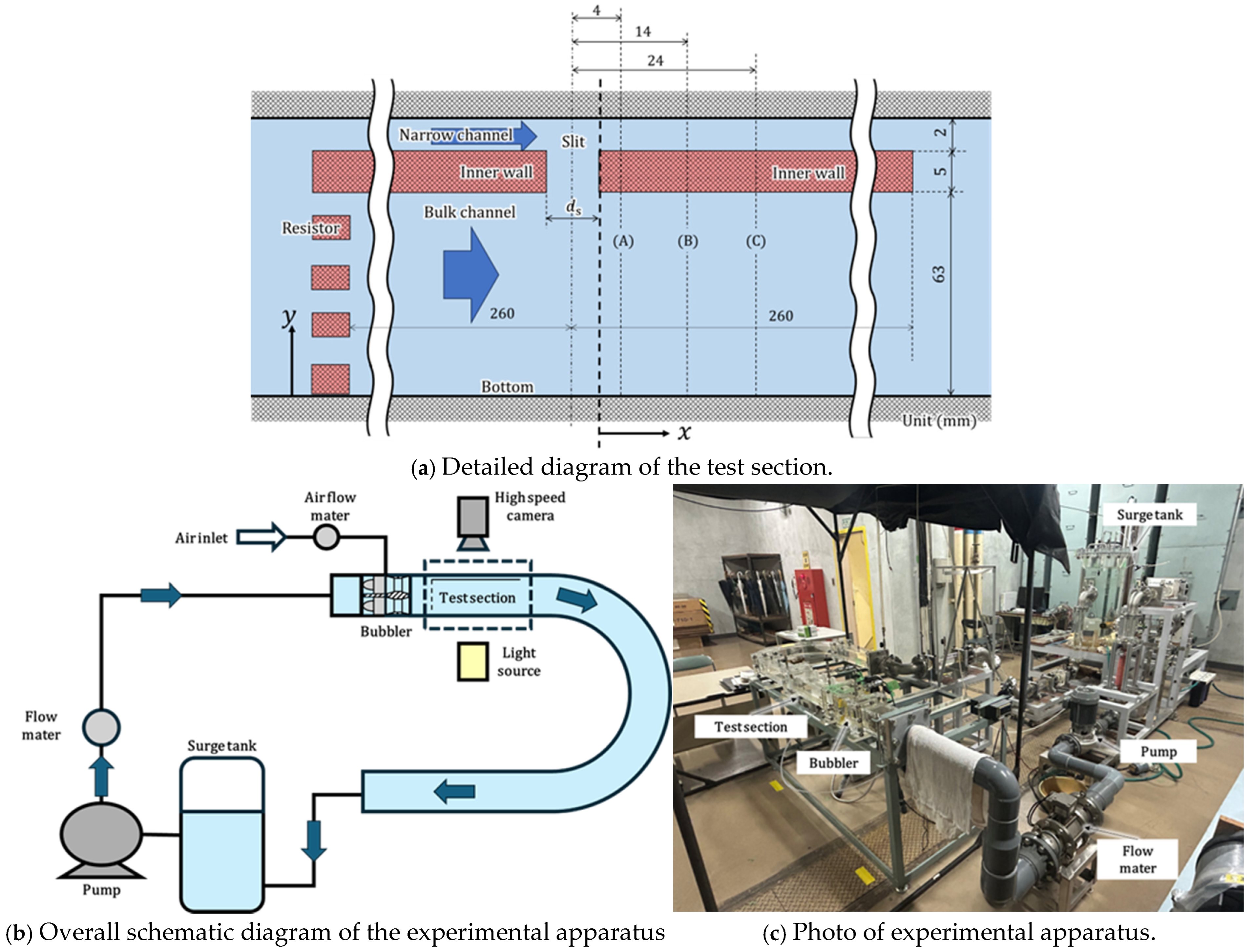
Figure 1 shows a schematic diagram of the experimental apparatus for visualizing JICF from the slit, simulating damage in the inner wall between the narrow and the main flow channels. Figure 1a shows a schematic diagram of a test section. The cross-section of the test section is 70 × 70 mm. The test section length is 520 mm. An inner wall with a slit to divide the test section into the main flow channel and the narrow flow channel was inserted. The slit was installed at the center of the test section. A resistor was installed upstream on the main flow channel to achieve a fast-speed narrow flow channel and a slow-speed main flow channel. The inner wall is 5 mm thick, dividing the test section into a narrow flow channel of 2 mm wide and a main flow channel of 63 mm wide. Owing to this geometry and the resistor set upstream of the main channel, the flow rate in the main channel is 50 times higher than at the narrow flow channel. The flow branched at the test section inlet converges at the test section outlet. The slit is provided in the inner wall at 260 mm from the test section inlet to the center of the slit. The slit width, $d_s$, was varied by replacing the inner wall. The slit width $d_s$ was set to $d_s$ = 2, 4, 6, and 8 mm. Water was used as the test fluid. Figure 1b,c show the overall experimental apparatus as a schematic diagram and photograph, respectively. A pump was installed upstream of the test section. The flow rate can be controlled by an inverter. A flowmeter was set downstream of the pump to maintain a constant flow rate in the test section. Additionally, a swirl bubbler [6] was installed upstream of the test section to generate air microbubbles, which served as a tracer for PIV measurement. The air flow rate for microbubble generation was controlled by a mass flow controller so that its ratio to the water flow rate is from 0.00115 to 0.00125. The test section is made of acrylic. The experiment was conducted by varying the slit width d_s and the water flow rate $Q_w$. The water flow rate $Q_w$ was set to $Q_w$ = 150, 175, 200, 225, and 250 L/min. The flow rate fluctuation during the test was within ±1%. A high-speed camera for capturing the flow field was mounted on the top surface shown in Figure 1a.

The experiment was conducted by the following procedure:

• Fill the experimental loop with water.
• Start the water flow. At this time, adjust the inverter output to achieve the set flow rate.
• Adjust the mass flow controller so that the air/water flow ratio is 0.0012 to inject air bubbles for the PIV tracer into the water.
• Take images of the flow conditions with the high-speed camera.

2.2. Flow Field Evaluation Using PIV

Particle Image Velocimetry (PIV) was applied to the captured video to visualize the flow of the JICF. For the tracer, microbubbles of air generated by a bubbler [6] installed upstream of the test section were used. The radius of the microbubbles ranged from 30 to 150 μm, with the peak of the number density distribution at 60 μm. It is noted that the behavior of these microbubbles was not investigated in this experiment. The video used for PIV was captured at a time interval of 333.33 μs, with 256 frames (equivalent to approximately 85 ms) and an image size of 250 × 400 pixels (equivalent to 18 mm × 28.8 mm: 72 mm/pixel). In this PIV process, the exploration region and the inspection region sizes were set to 32 × 32 and 15 × 15 pixels, respectively. In the PIV measurements, the number of microbubbles was 3 to 4 in the measurement area. For image processing, a wall and background were deleted from the image to eliminate those influences. Vectors in the regions where the exploration area overlapped with the wall and where they extended beyond the image were deleted. Furthermore, velocity vectors with a correlation coefficient of 0.5 or lower were removed and then interpolated from the surrounding vectors. PIV provides results for each frame, but to suppress variations for each frame, the results for each frame were averaged. The uncertainty in the velocity of this measurement system is ±0.03 m/s when evaluated at a 95% confidence level [9]. For PIV measurements that are not affected by time variations in the flow due to turbulence, it is necessary to use an average over enough frames. In this experimental setup, at locations not influenced by the jet (upstream in the x-direction from the slit), the average of the y-direction velocity over 256 frames must be 0 m/s. In the present measurement, the average y-direction velocity over 256 frames upstream in the x-direction from the slit at a location not influenced by the jet (x = −26 mm, y = 41 mm) was approximately 0.012 m/s. Considering the uncertainty of the measurement system, this can be regarded as 0 m/s, indicating that the measurement sufficiently suppresses velocity fluctuations due to turbulent phenomena.

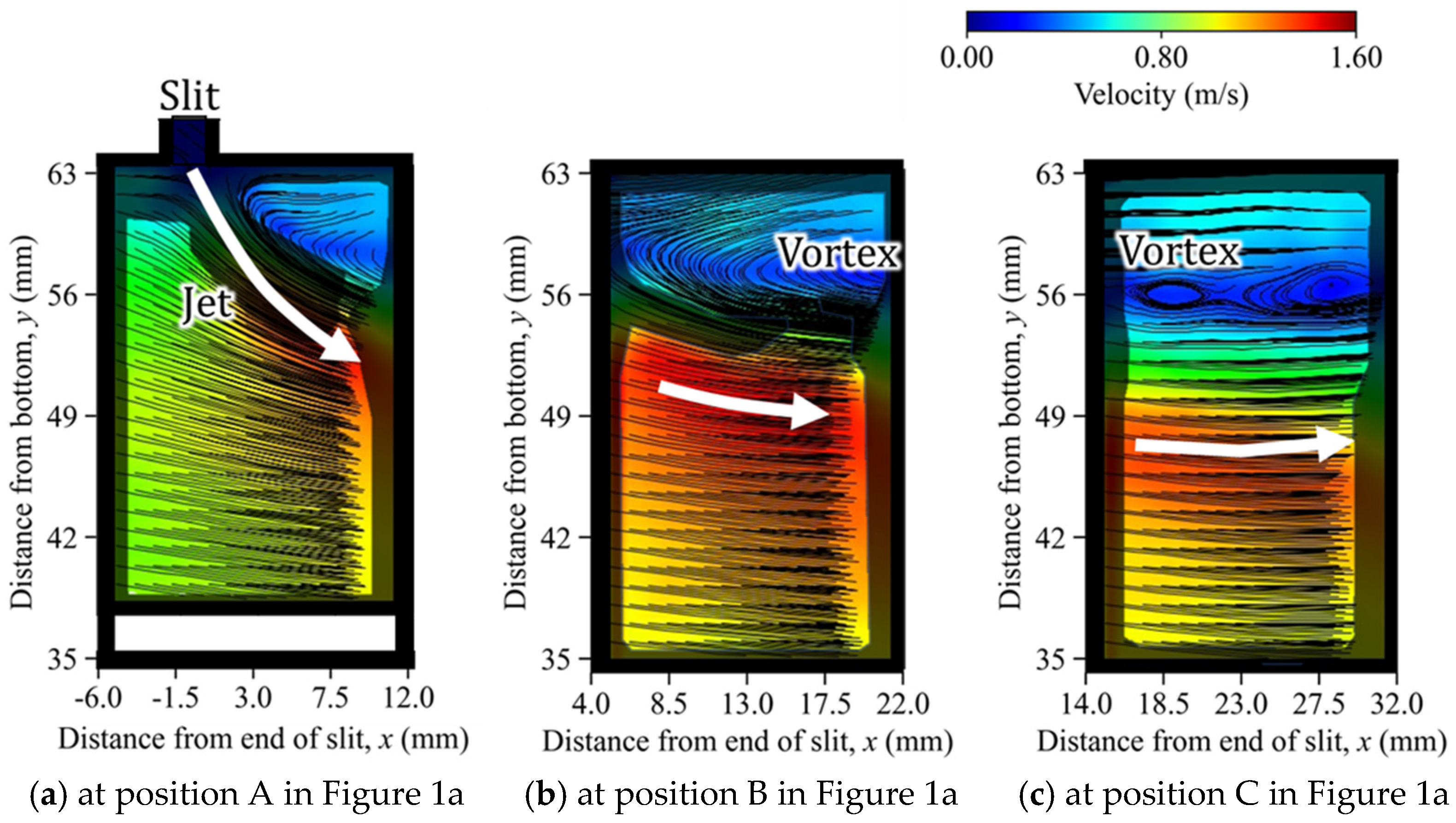
Regarding the location of taking the image, the center positions of the image were set at (A), (B), and (C), as shown in Figure 1a, which correspond to positions of 4, 14, and 24 mm downstream from the slit center in the mainstream direction (the x-direction in Figure 1a), respectively.

In this measurement, the concentration of bubbles, which are tracer particles of PIV, near the slit resulted in a poor cross-correlation coefficient for estimating the migration of tracer particles. Therefore, only the region where the normalized cross-correlation coefficient was 0.5 or higher is displayed in the measurement results.

3. Numerical Analysis

3.1. Modeling the Phenomenon

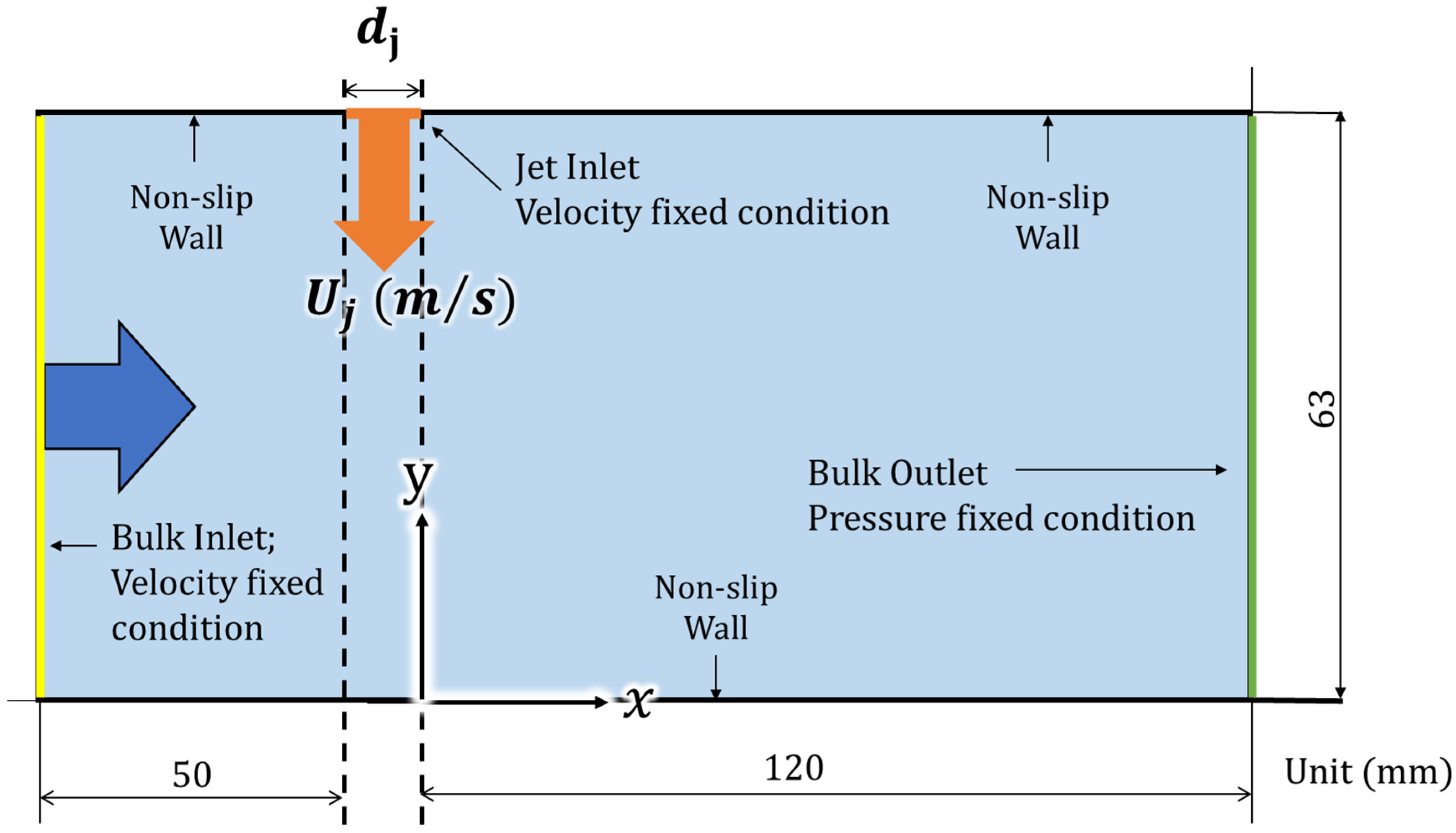
PIV experimental results (details in 4.1) indicate that the flow from the slit to the main flow channel resembles a JICF. Furthermore, the width and velocity of the jet vary depending on the slit width and the velocity difference between the main flow and the narrow flow channel. Therefore, a numerical analysis simulating the experimental JICF into the main flow, as shown in Figure 2, was conducted. In the analysis, the jet was simulated as a flow perpendicular to the main flow. The inlet jet velocity denoted as $U_j$ and the inlet width of the jet as $d_j$ were varied to evaluate the effect of $U_j$ and $d_j$ on the pressure fluctuations in the main flow. Note that this model cannot consider the phenomenon where flow from the main channel enters the narrow channel.

3.2. Simulation Analysis Method

The analysis employed the open-source analysis software OpenForm v1806 [10], utilizing the PimpleForm solver [11]. The governing equations in PimpleFoam are the Continuity Equation (1) and the Navier–Stokes (N-S) Equation (2) for incompressible fluids.

$$\nabla ·\mathit{U}=0,$$

(1)

$${\displaystyle \frac{\partial \mathit{U}}{\partial t}}+\nabla ·\left(\mathit{U}⨂\mathit{U}\right)=-{\displaystyle \frac{1}{\rho }}\nabla p+{\mathsf{\nu }\nabla }^2\mathit{U}.$$

(2)

where $U$ is the velocity, $p$ is the pressure, and $\nu$ is the kinematic viscosity. The solver employs the finite volume method for discretization. Pressure and velocity are coupled using the PISO method [11].

The flow inside the mercury target vessel is a high Reynolds number flow, necessitating the use of a turbulence model. In this study, it is crucial that the model accurately accounts for wall effects and is applicable to the high Reynolds number regime. Furthermore, a RANS model was selected since this study focuses on the pressure drop in the field rather than the time-dependent vortices caused by turbulence. Regarding RANS models, Di Zhang verified the accuracy of the k-ωSST model for flow around a cylinder and reported its good performance [12]. Furthermore, Ramponi et al. analyzed cross-ventilation in buildings and demonstrated that the k-ωSST model exhibited the highest accuracy when compared to several other models [13]. Therefore, the k-ωSST model, a type of RANS model, was selected as the turbulence model. The k-ωSST model implemented in OpenFoam is based on the model by F.R. Menter et al. [14] and is characterized by its ability to accurately compute flow fields where both low and high Reynolds number regions coexist. In the k-ωSST model, the turbulent dissipation rate ω is given by Equation (3) below, and the turbulent kinetic energy k is given by Equation (4).

$$\frac{D}{Dt}\left(\rho \omega \right)=\nabla ·\left(\rho D_{\omega }\nabla \omega \right)+\frac{\rho \gamma G}{\nu }-\frac{2}{3}\rho \gamma \omega \left(\nabla ·U\right)-\rho \beta {*\omega }^2-\rho \left(F_1-1\right)C{D}_{k\omega }+S_{\omega }$$

(3)

$${\displaystyle \frac{D}{Dt}}\left(\rho k\right)=\nabla ·\left(\rho D_k\nabla k\right)+\rho G-{\displaystyle \frac{2}{3}}\rho k\left(\nabla ·U\right)-\rho {\beta }^{*}\omega k+S_k$$

(4)

The turbulent viscosity coefficient ${\nu }_t$ was obtained using the following Equation (5) with $k$ and $\omega$ derived from these equations.

$${\nu }_t=a_1{\displaystyle \frac{k}{\max \left(a_1\omega ,b_1{F}_{2}S\right)}}$$

(5)

where ${\alpha }_{k1}, {\alpha }_{k2}, {\alpha }_{\omega 1}, {\alpha }_{\omega 2}, {\beta }_1, {\beta }_2, {\gamma }_1, {\gamma }_2, {\beta }^{*}, a_1, b_1, c_1$ are constants, and recommended values [15] were used.

Numerical analyses were conducted for water and mercury. The physical properties used in PimpleFoam are density and the kinematic viscosity coefficient. In

Table 1. Density and kinematic viscosity in standard conditions.

	Density, $\mathit{\rho } \left[\mathbf{k}\mathbf{g}/{\mathbf{m}}^3\right]$	$\mathbf{Kinematic}\mathbf{Viscosity},\mathit{\nu } [{\mathbf{m}}^2/\mathbf{s}]$
Water	1000	$0.90\times {10}^{-6}$
Mercury	13,500	$0.11\times {10}^{-6}$

, those values used in this analysis are shown. In addition, the Reynolds numbers for water and mercury are 70,000 and 570,000, respectively, in these analyses. y+ in the analyses for water and mercury are 5~30 and 50~240, respectively.

3.3. Analysis System and Conditions

Numerical analyses were conducted with the model shown in Figure 2. The jet was entered perpendicular to the mainstream flow based on the experimental results presented in Section 4. The inlet of the main flow channel was set as a fixed velocity boundary condition. The outlet was set as a fixed pressure condition at 105 Pa. All walls were set as wall boundary conditions. The jet flow was injected from the jet inlet shown in Figure 2 under a fixed velocity condition. The jet velocity $U_j$ and jet width $d_j$ were varied to evaluate the jet’s influence. To examine the dependence on mesh size, the number of mesh divisions in the analysis system was changed, and analyses were conducted. Between approximately 80,000 and 135,000 mesh divisions, the error in the analysis results (for example, pressure) was about 30%. On the other hand, between approximately 135,000 and 200,000 mesh divisions, the error decreased to about 7%, which indicated that the mesh division number is sufficient to ensure grid independence. In the present analysis, considering computational efficiency, the mesh was set to approximately 135,000 divisions.

As shown in the experimental results described later, the jet velocity $U_j$ and width $d_j$ flowing from the narrow channel into the main channel vary depending on the experimental conditions. This is thought to be due to changes in the pressure difference between the main flow and the narrow flow channels. For the mercury target, this pressure difference varies due to various factors such as thermal expansion, pressure waves, and cavitation caused by the incident proton beam. For this reason, various patterns of jet velocity $U_j$ and width $d_j$ are used for analyses. In the numerical analyses, the flow velocity $U_j$ was set to $U_j$ = 1, 2, 3, 4, 5 and 10 m/s. The jet width $d_j$ was varied from 0.5 mm to 6.0 mm. The jet velocity $U_j$ was varied from 0.3 m/s to 10 m/s.

4. Results

4.1. Flow Field Measured by PIV

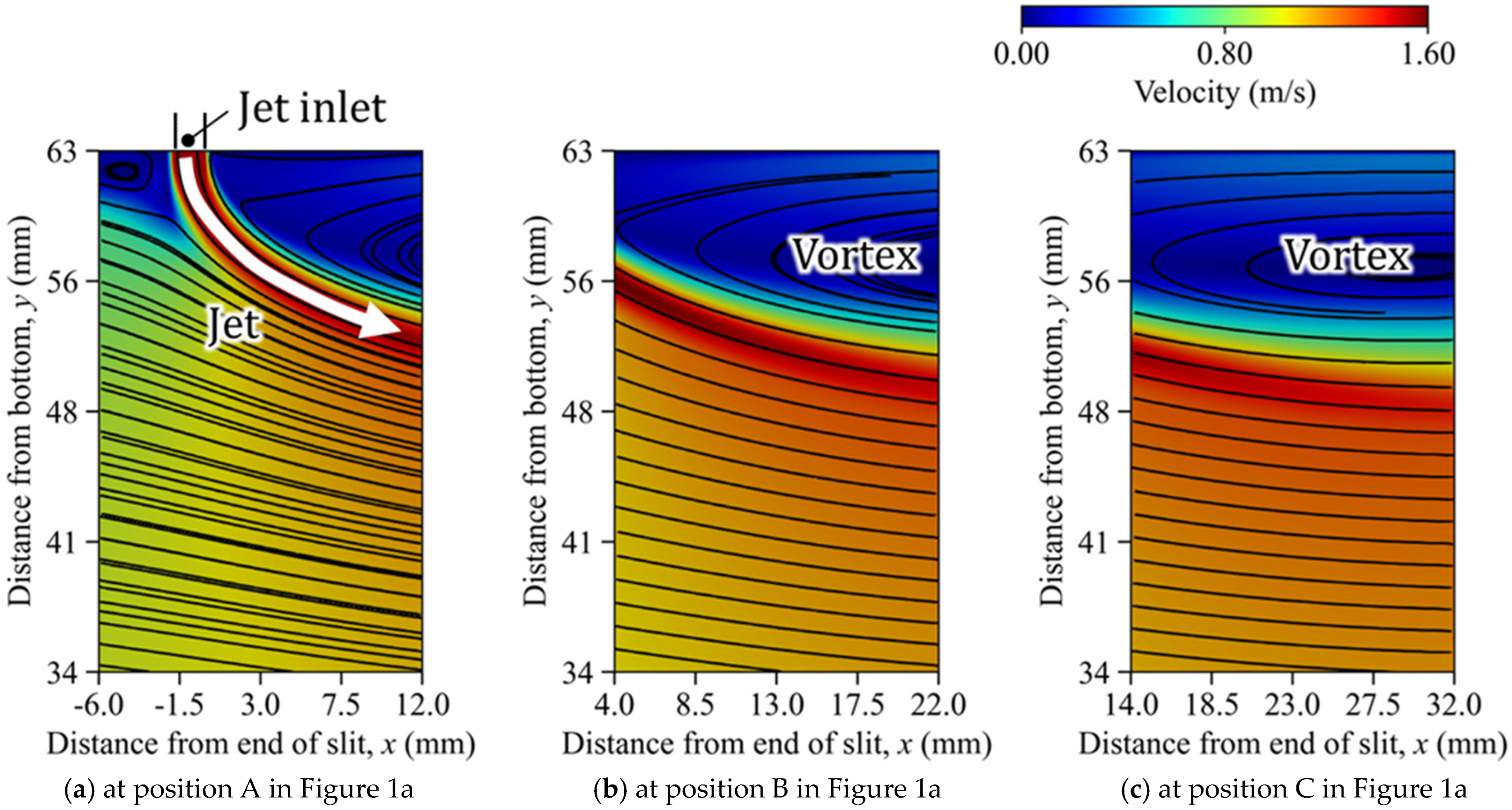
Figure 3a–c show PIV results of streamline on the velocity distributions at observation positions (A) to (C), respectively, for a slit width $d_s$ = 2 mm and water flow rate $Q_w$ = 250 L/min. Regions with the normalized cross-correlation coefficient of 0.5 or less were filled in. The velocity in the main flow channel is approximately 0.85 m/s. Streamlines extend from the slit toward the main flow channel, forming the JICF. Unfortunately, the normalized cross-correlation coefficient was 0.5 or less near the slit. Figure 4 shows the results near the slit when the flow rate was reduced to Q_w = 150 L/min. A jet flow is generated, which is thought to be flowing in from the slit, and it is considered to be forming a JICF. The flow pattern in the region with a correlation coefficient of 0.5 or more in Figure 3a is similar to that in Figure 4, and it is considered that a JICF is being formed by a jet flow from the slit. Furthermore, in the downstream area shown in Figure 3b, the jet flow in the main flow channel bends along the direction of the main flow. Meanwhile, the flow in the main channel moves downward in the image; i.e., it is pushed downward by the jet. Further downstream in Figure 3c, the jet’s speed decreases while changing direction towards the top of the image. These flows generate large vortices on the inner wall side of the main channel downstream of the slit.

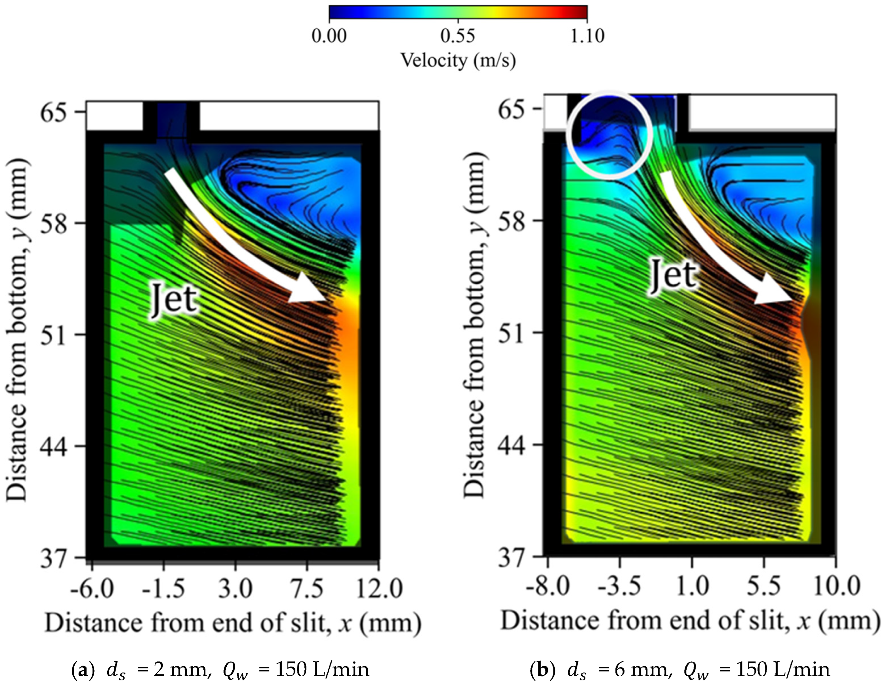
Figure 4a,b show the velocity distribution at measurement position (A) varying the $d_s$ and $Q_w$. Figure 4a shows the result under the condition of $d_s$ = 2 mm and $Q_w$ = 150 L/min. The flow pattern is very similar to Figure 3a, although the velocity is different. However, as shown in Figure 4b, when $d_s$ is wider, such as 6 mm, the flow direction from the main channel to the slit can be observed upstream of the main flow within the slit. This is thought to occur because flow separation occurs upstream within the slit due to the high-velocity flow in the narrow channel, causing a pressure drop. And due to the pressure drop within the slit, the water of the main channel is drawn into the slit.

4.2. Flow Field Simulation

To verify the analysis results, a comparison was made between the experimental and analysis results. In the analysis, the jet velocity $U_j$ is defined as the velocity at which the pressure drop across the slit, treating it as a flow path, equals the pressure difference incurred by the fluid in the main flow and narrow flow channels. This pressure difference corresponds to the pressure drop associated with the flow velocity in each path.

The comparison analysis was performed under the condition of $d_j$ = 2 mm and $U_j$ = 1.5 m/s, which corresponds to the experiment under $d_s$ = 2 mm and $Q_w$ = 250 L/min (Figure 3). Figure 5a–c show the analysis results for velocity distribution scaled to the same dimensions as Figure 3a–c. Comparing Figure 5a with Figure 3a, the jet bends downstream within the main channel, and the flow in the main channel is reproduced as downward in the image; i.e., the flow displaced by the jet flow as seen in the experiment. Additionally, comparing Figure 5b,c with Figure 3b,c, in the downstream region of the JICF, a large vortex forms near the inner wall of the main channel, consistent with the PIV results.

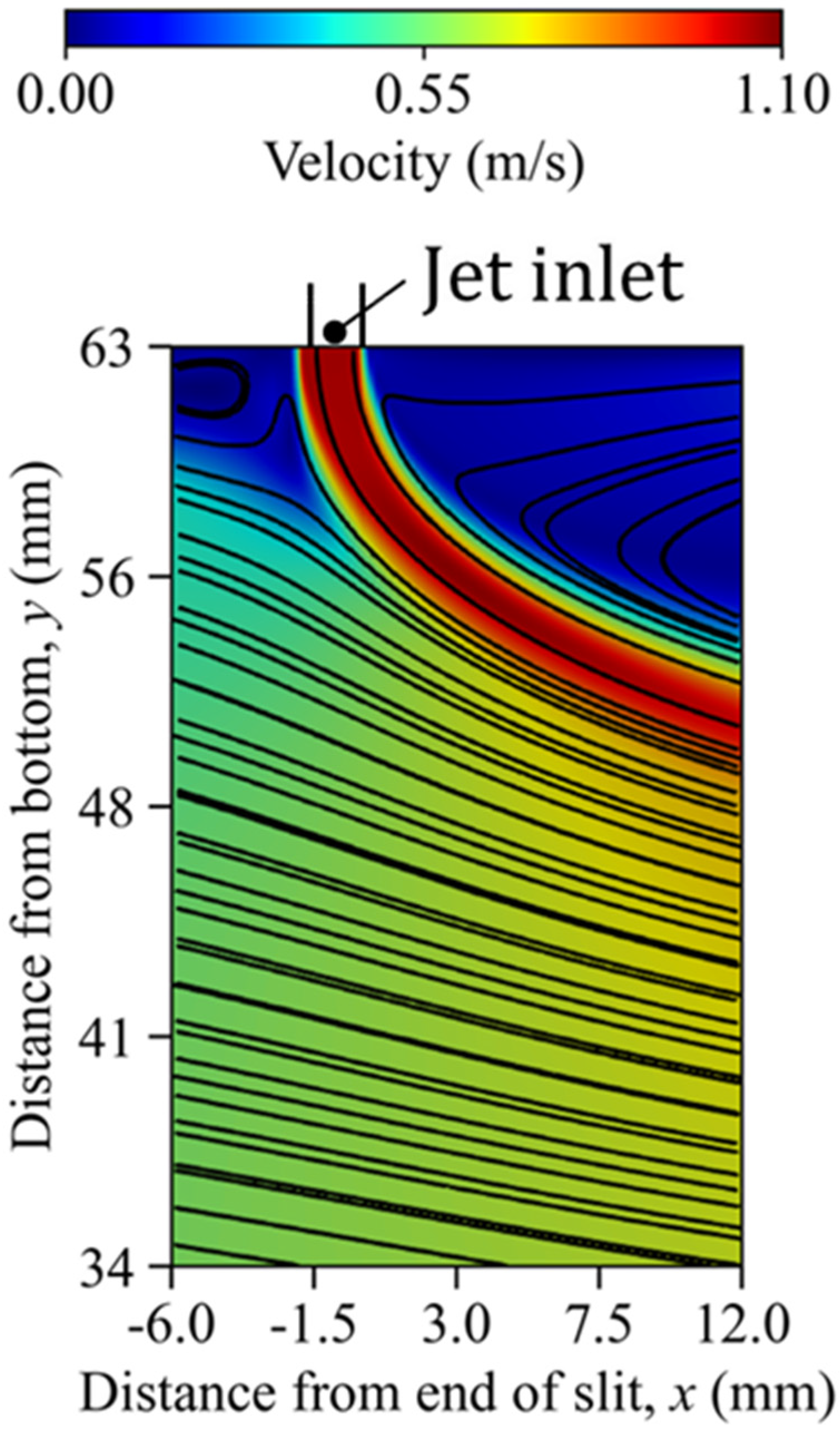
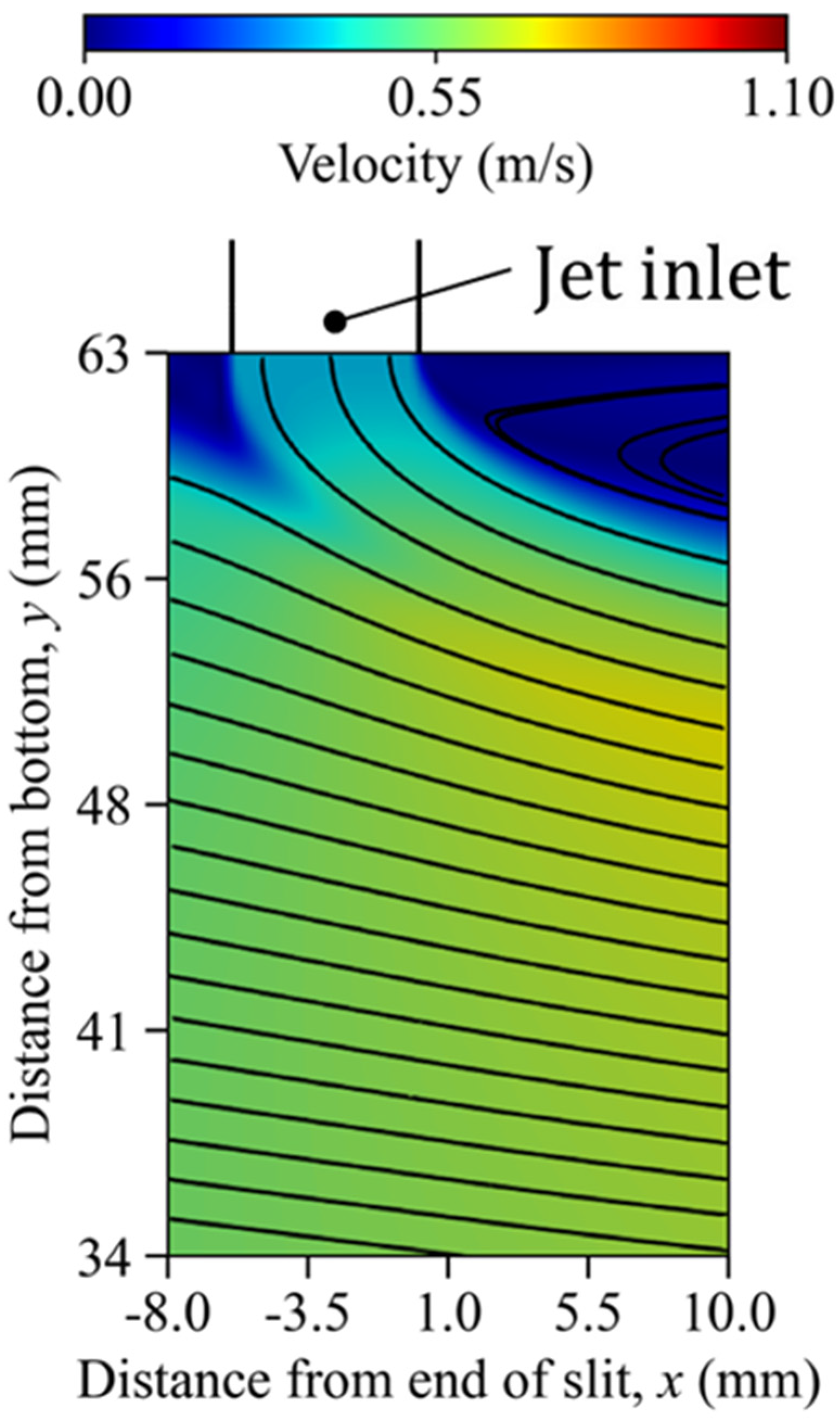
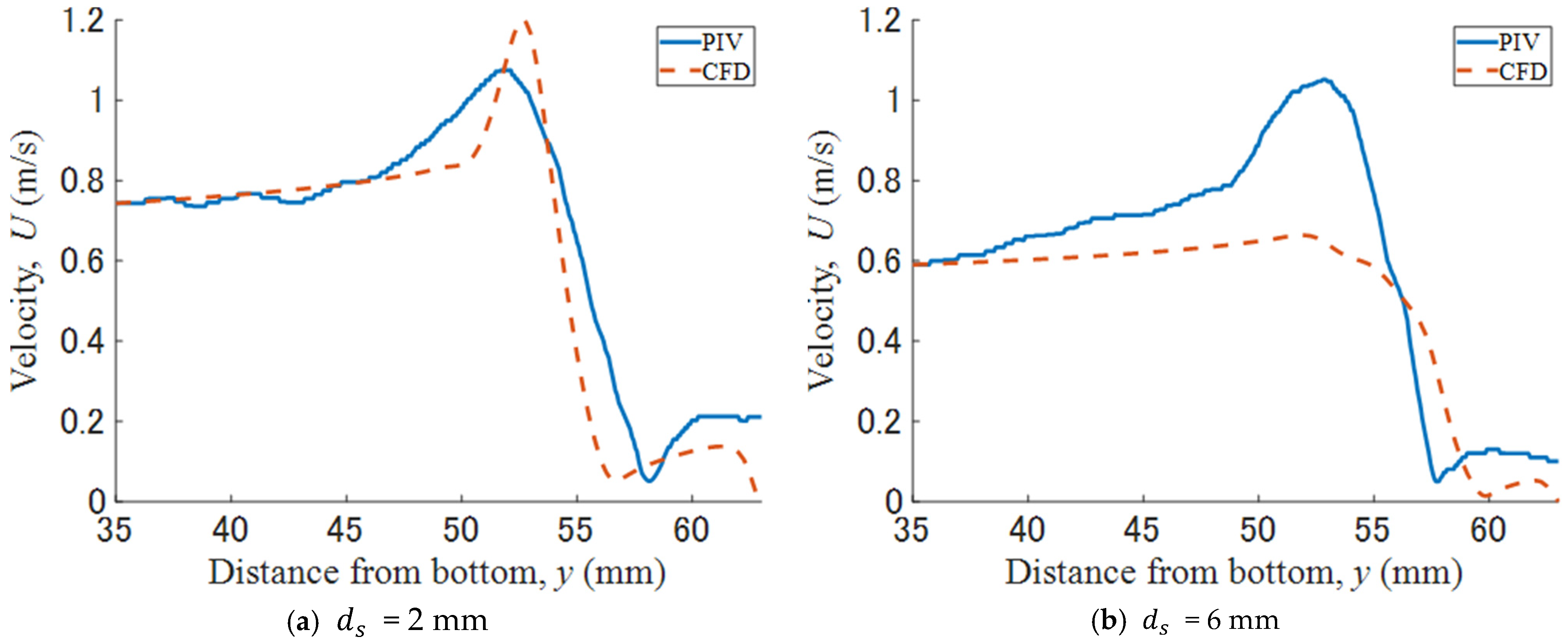
Figure 6 shows the analysis results under the condition of $U_j$ = 1.02 m/s and $d_j$ = 2 mm to compare Figure 4a. Figure 7 shows the analysis results under the condition of $U_j$ = 0.34 m/s and $d_j$ = 6 mm to compare to Figure 4b. For the jet width $d_j$ = 2 mm shown in Figure 6, a velocity distribution equivalent to the experimental results was obtained. On the other hand, in the experiment with $d_s$ = 6 mm, backflow from the main flow occurs within the upstream slit, narrowing the jet width. For $d_j$ = 6 mm, assuming $d_s$ = 6 mm, as shown in Figure 7, not only did the flow velocity values differ but so did their distribution. It fails to reproduce the narrowing of the jet width caused by backflow when the slit width increases. To validate the analysis results for d_s = 2 mm, the results were compared with the PIV results. Figure 8 shows the velocity distribution along the y-direction at x = 8 mm. Figure 8a shows a comparison of the velocity distributions for the case where $d_s$ = 2 mm. The results of the numerical analysis not only reproduce the maximum velocity observed by PIV around y = 53 mm but also capture the minimum velocity caused by the vortex around y = 63 mm. On the other hand, in the case of $d_s$ = 6 mm shown in Figure 8b, in the analysis, $d_j$ is assumed to be equal to $d_s$, which results in a slower jet velocity, and the maximum velocity is about 2/3 of the PIV results. To evaluate the validity of the velocity distribution of the analysis results, the root mean square error (RMSE) against the PIV velocity distribution was used as an indicator, and the RMSE was evaluated from the velocities at each position in the y-direction. In the case of $d_s$ = 2 mm, where no backflow occurred in the PIV, and in the cases of $d_s$ = 4, 6, and 8 mm, where backflow occurred, the RMSE values were 0.164, 0.212, 0.273, and 0.203, respectively. From these results, it can be considered that for $d_s$ ≤ 2 mm, the analysis results are relatively reasonable, although it is unclear whether backflow occurs into the slit.

5. Discussion—Pressure Fluctuation and Cavitation

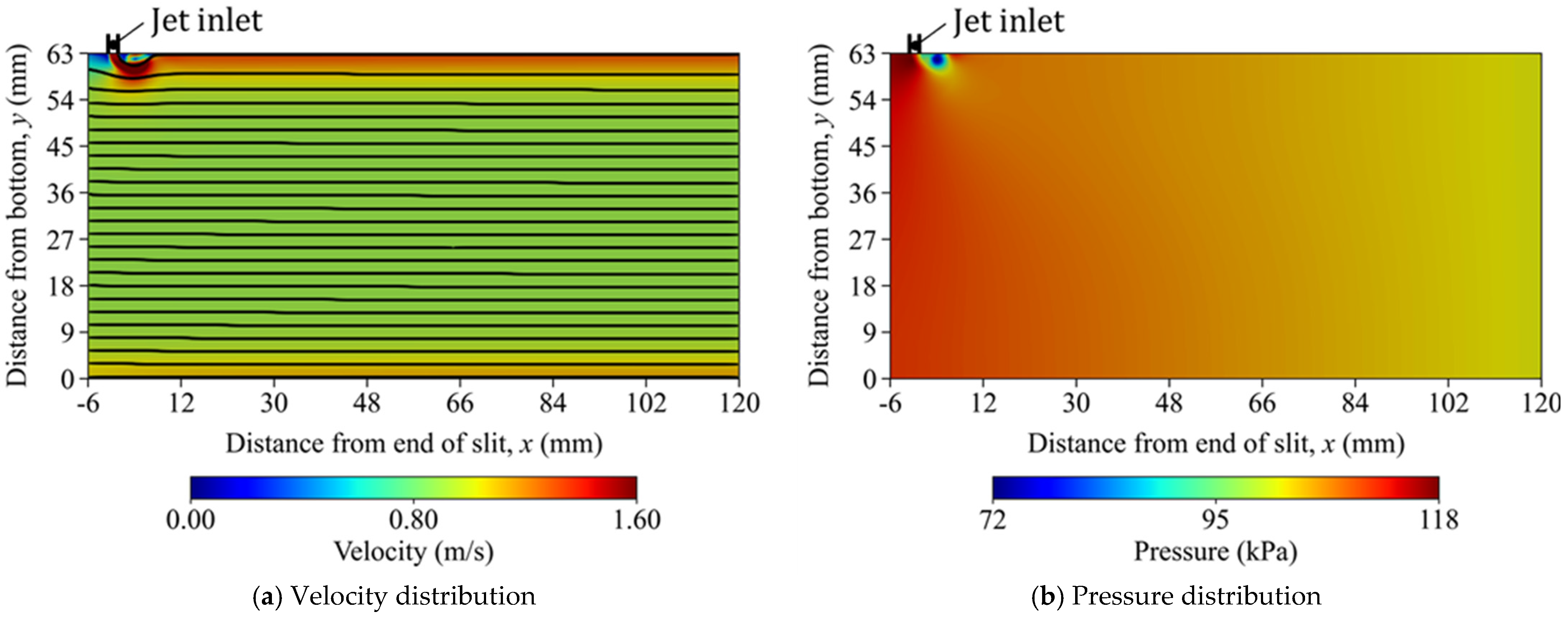
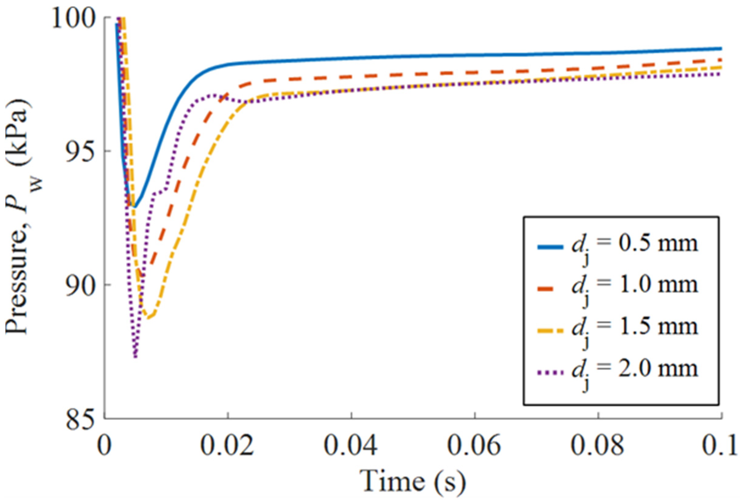
When pressure decreases due to flow field disturbance caused by the jet, cavitation can occur. Upon pressure recovery, the cavitation bubble contracts and collapses while releasing local shock pressure. Since the released local shock damages the material, the pressure field caused by the JICF was evaluated. Figure 9a,b show the velocity distribution and pressure distribution, respectively, at the time when the lowest pressure occurred in the analysis for water. The lowest pressure occurred at 14 ms after the jet began entering the main flow (beginning of the analysis). The conditions are $d_j$ = 2 mm, $U_j$ = 1.02 m/s (corresponding to $d_s$ = 2 mm, $Q_w$ = 250 L/min). The lowest pressure appears downstream of the slit, where a small vortex is generated owing to starting JICF, as shown in Figure 9a (x = 1.75 mm, y = 62 mm). Figure 10 shows the time history of pressure at the location (x = 1.75 mm, y = 62 mm) where the lowest pressure appeared under the condition of $=4$ m/s and $d_j\le$ 2 mm. After the jet begins entering the main flow channel (t = 0 s), the pressure decreases rapidly, reaching the minimum at t = 14 ms. Subsequently, the pressure recovers and converges to a constant value. Although the pressure value at this decrease is not extremely low, it indicates that the pressure fluctuation causes bubble expansion, contraction, and collapse, suggesting the potential for material damage.

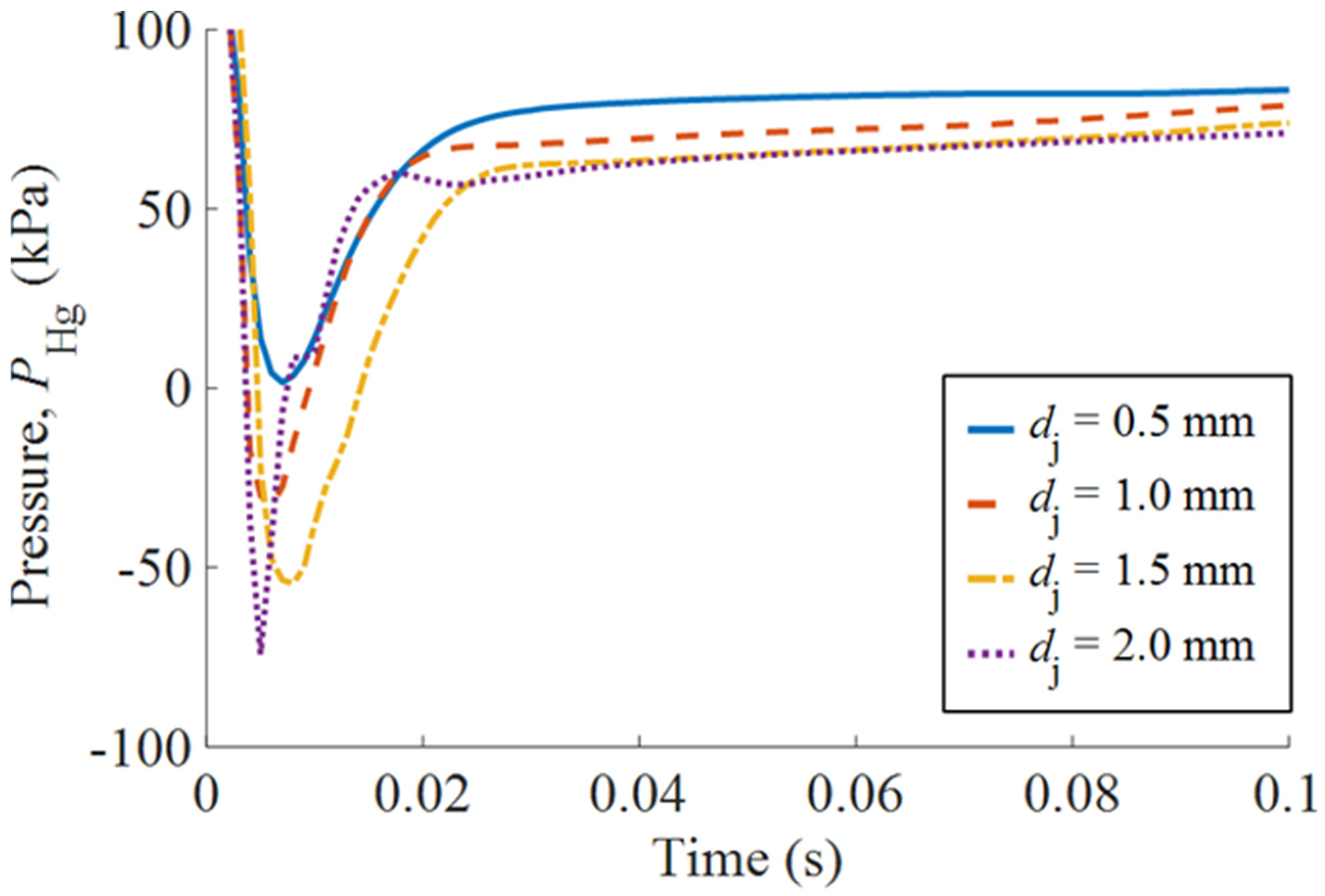
Since the density of mercury is 13.5 times greater than that of water, larger pressure fluctuations are expected. Therefore, pressure fluctuations due to the JICF in mercury were evaluated. Figure 11 shows the pressure history in mercury at x = 2.5 mm and y = 62 mm, which is near the outlet of the slit and near the top wall of the main channel. The minimum pressure is significantly lower than that for water, and the pressure decrease is about 13.5 times greater. On the other hand, the pressure fluctuation trend showed little difference between water and mercury. Also, when the jet velocity, $U_j$ is the same, the larger the jet width, $d_j$, the greater the pressure drop at the initial stage of JICF.

The inflow of the jet causes a sudden drop in pressure, and cavitation is expected to occur. The time variation in the cavitation number $\sigma$ at the location shown in the pressure history in Figure 11 was evaluated using Equation (6). Except for $d_j$ = 0.5 mm, the cavitation number, $\sigma$ is less than or equal to zero, indicating the possibility of cavitation.

$$\sigma ={\displaystyle \frac{p\left(t\right)-p_v}{0.5\rho U^2}}$$

(6)

Therefore, the possibility of bubble expansion and collapse due to the JICF was examined using the Rayleigh–Plesset equation (R-P equation, Equation (7)) using the pressure history at the position where the minimum pressure appeared in the analysis as input conditions.

$$\ddot{R}+{\displaystyle \frac{3}{2}}{\dot{R}}^2={\displaystyle \frac{1}{\rho }}\left\{p_g\left(R\right)-p\left(t\right)-p_v-{\displaystyle \frac{4\mu \dot{R}}{R}}-{\displaystyle \frac{2\kappa }{R}}\right\}$$

(7)

where, $p_g\left(R\right)$ is the pressure inside the bubble estimated by Equation (8), $p\left(t\right)$ is the pressure at the bubble interface, which is the pressure history obtained by the analysis, as shown in Figure 10, $p_v$ is the saturated vapor pressure, and $\kappa$ is the surface tension.

$$p_g\left(R\right)=\left(p_{\mathrm{\infty },0}-p_v+{\displaystyle \frac{2\kappa }{R_0}}\right){\left({\displaystyle \frac{R_0}{R}}\right)}^{3\gamma }$$

(8)

where, $p_{\mathrm{\infty },0}$ is the initial pressure and $\gamma$ is the ratio of specific heat of gas.

Table 2. Physical properties and initial pressure used in Equation (7).

	Saturated Vapor Pressure, ${\mathit{p}}_{\mathit{v}}$ [kPa]	Surface Tension, $\mathit{\kappa }$ [N/m]	Ratio of Specific Heat, $\mathit{\gamma }$	Initial Pressure, ${\mathit{p}}_{\mathbf{\infty },0}$ [kPa]
Mercury	$0.16\times {10}^{-3}$	0.48	-	100
Helium	-	-	1.67	-

shows the properties used in this calculation.

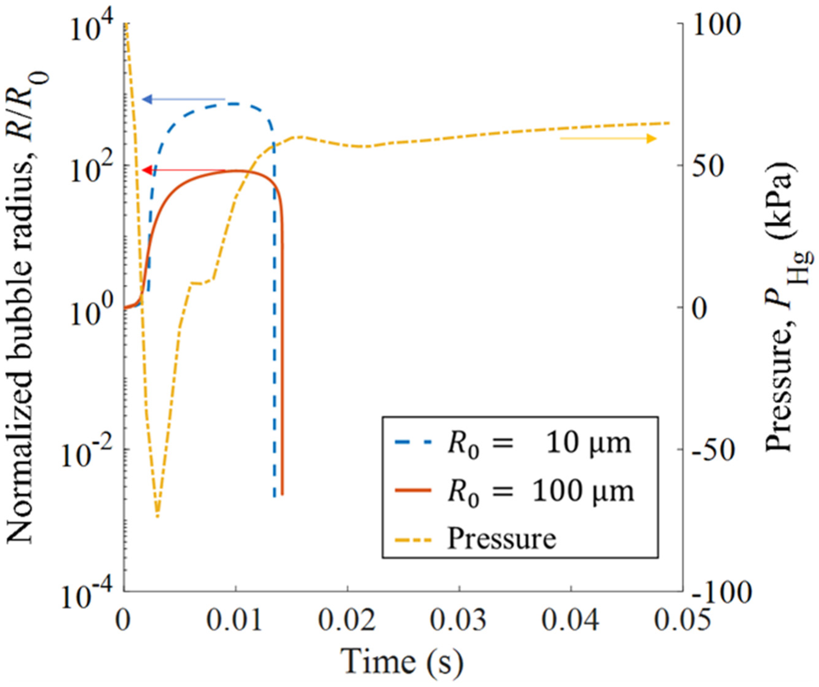
Figure 12 shows bubble behavior and pressure history under the case of jet width $d_j$ = 2 mm and jet velocity $U_j$ = 4 m/s. Initial bubble radii were evaluated for R0 = 10 μm, simulating a cavitation nucleus, and R0 = 100 μm, simulating a gas bubble injected into a mercury target. For both of the bubble radii, the bubble expands as the pressure decreases. After this, the bubble continues to expand owing to the inertia, although pressure p(t) is recovered. And then, however, the bubble begins to contract rapidly. This result suggests that damage could occur downstream of the slit due to pressure fluctuations caused by the JICF, which is generated by the penetration of the inner wall between two parallel flow channels. For water, it is noted that the pressure decrease was too small to cause bubble expansion and contraction.

This result reproduces the beginning stage of the flow of the JICF, i.e., immediately after penetration. However, a similar phenomenon, i.e., the increase in the jet velocity, could occur in the mercury target vessel. In the mercury target vessel, gas bubbles are injected into the main flow channel to reduce pressure waves. Consequently, owing to the proton beam injection, the generated pressure in the narrow flow channel is approximately three times higher than in the main flow channel [7]. This pressure difference can readily generate a JICF, accelerating damage.

As the penetration area owing to the cavitation damage in the inner wall between the narrow flow and the main flow channels expands, it becomes impossible for the narrow flow channel to keep its function. Then, damage to the outer wall of the narrow flow channel becomes severe, ultimately posing a risk of mercury leakage. Therefore, the development of methods to accurately evaluate damage to the inner wall and to detect such damage is expected. The impact load caused by bubble collapse owing to pressure fluctuations induced by the JICF could be a significant phenomenon for detecting inner wall penetration.

6. Concluding Remarks

We clarified the flow pattern when penetration damage occurs on the inner wall between two parallel flows through experiments and analyses and considered the possibility of cavitation generation due to pressure fluctuations in that case. Cavitation initiated by penetration damage is a phenomenon that should be considered, especially when evaluating the lifespan of mercury target containers with high precision. The findings obtained in this study are as follows:

(1)

The JICF is generated, flowing from the narrow channel through the slit into the main channel. The JICF in the main channel generates vortices near the inner wall of the main channel downstream of the slit. The numerical simulation, in which only the jet width and jet velocity were simulated, reproduces the flow pattern of the JICF, especially for the slit width $d_s$ = 2 mm. It is noted that the jet width could not be the same as the slit when $d_s$ > 2 mm.

(2)

The simulation revealed that pressure decreased rapidly near the inner wall downstream of the jet inlet at the beginning of the JICF. This beginning corresponds to the moments when the inner wall is penetrated and/or when the pressure difference between the narrow flow and the main flow channels increases. In the mercury target vessel, a pressure difference could occur when the pressure wave is generated during pulsed proton beam injection because the pressure wave generated in the narrow flow channel is higher than that in the main flow channel, where the pressure wave is reduced by bubbles.

(3)

The possibility of cavitation damage due to the pressure fluctuation induced by the JICF in mercury was shown by the Rayleigh–Plesset calculation. This suggests that damage could accelerate due to the JICF, which is generated by penetration of the inner wall in the mercury target vessels.

(4)

Based on these findings, the vibration of the target vessel caused by localized pressure owing to cavitation collapse induced by the JICF, which would appear after penetration of the inner wall, could be used for anomaly diagnosis.

References

1. Bhatia, B.; Johny, T.; De, A. Understanding the liquid jet break-up in various regimes at elevated pressure using a compressible VOF-LPT coupled framework. Int. J. Multiph. Flow 2023, 159, 104303. [Google Scholar] [CrossRef]
2. Meftah, M.B.; Mossa, M. Turbulence Measurement of Vertical Dense Jets in Crossflow. Water 2018, 10, 286. [Google Scholar] [CrossRef]
3. Wang, L.; Wu, W.; Li, X.; Fan, S.; Fang, Z. Coupling mechanism of structure–cavitation impact in reflux self-excited oscillating nozzles. Ocean Eng. 2025, 332, 121355. [Google Scholar] [CrossRef]
4. Available online: https://neutrons.ornl.gov/ (accessed on 20 September 2024).
5. Available online: https://j-parc.jp/c/en/index.html (accessed on 20 September 2024).
6. Kogawa, H.; Naoe, T.; Kyotoh, H.; Haga, K.; Kinoshita, H.; Futakawa, M. Development of microbubble generator for suppression of pressure waves in mercury target of spallation source. J. Nucl. Sci. Technol. 2015, 52, 1461–1469. [Google Scholar] [CrossRef]
7. Kogawa, H.; Naoe, T.; Futakawa, M.; Haga, K.; Wakui, T.; Harada, M.; Takada, H. Mitigation technologies for damage induced by pressure waves in high-power mercury spallation neutron sources (IV)–measurement of pressure wave response and microbubble effect on mitigation in mercury target at J-PARC–. J. Nucl. Sci. Technol. 2017, 54, 733–741. [Google Scholar] [CrossRef]
8. McClintock, D.A.; Liu, Y.; Bruce, D.R.; Winder, D.E.; Schwarts, R.G.; Kyte, M.; Blockland, W.; Sagrey, W.B.; Carroll, T.M.; Long, C.D.; et al. Small-bubble gas injection to mitigate cavitation-induced erosion damage and reduce strain in target vessel at the Spallation Neutron Source. Mater. Des. 2022, 221, 110937. [Google Scholar] [CrossRef]
9. Okamot, T. Handbook of Particle Image Velocimetry, 1st ed.; Morikita Publishing Co., Ltd.: Tokyo, Japan, 2013; pp. 137–164. (In Japanese) [Google Scholar]
10. Available online: https://www.openfoam.com/ (accessed on 10 December 2025).
11. Issa, R.I. Solution of the implicitly discretised fluid flow equations by operator-splitting. J. Comput. Phys. 1986, 62, 40–65. [Google Scholar] [CrossRef]
12. Zhang, D. Comparison of Various Turbulence Models for Unsteady Flow around a Finite Circular Cylinder at Re=20000. J. Phys. Conf. Ser. 2017, 910, 012027. [Google Scholar] [CrossRef]
13. Ramponi, R.; Blocken, B. CFD simulation of cross-ventilation for a generic isolated building: Impact of computational parameters. Build. Environ. 2012, 53, 34–48. [Google Scholar] [CrossRef]
14. Menter, F.R.; Kuntz, M.; Langtry, R. Ten Years of Industrial Experience with the SST Turbulence Model. In Proceedings of the 4th International Symposium on Turbulence, Heat and Mass Transfer, Antalya, Turkey, 12–17 October 2023. [Google Scholar]
15. Available online: https://www.openfoam.com/documentation/guides/latest/doc/guide-applications-solvers-incompressible-pimpleFoam.html (accessed on 10 December 2025).
Figure 1. Experimental apparatus of (a) detailed diagram of the test section. (b) Schematic diagram of the overall experimental apparatus and (c) photograph of the overall of the experimental apparatus.
Fluids 11 00097 g001
Figure 2. Numerical simulation model.
Fluids 11 00097 g002
Figure 3. Flow velocity distributions and streamlines obtained by PIV at positions (a) (A), (b) (B), and (c) (C) in Figure 1a under the condition of d s = 2 mm, Q w = 250 L/min.
Fluids 11 00097 g003
Figure 4. Flow velocity distributions and streamlines obtained by PIV at position A under the condition of (a) d s = 2 mm, Q w = 150 L/min and (b) d s = 6 mm, Q w = 150 L/min.
Fluids 11 00097 g004
Figure 5. Analysis results for the velocity distribution and streamline at positions (a) A, (b) B, and (c) C in Figure 1b under the condition of d j = 2 mm, U j = 1.5 m/s, which corresponds to d s = 2 mm, Q w = 250 L/min.
Fluids 11 00097 g005
Figure 6. Analysis results under the condition of U j = 1.02 m/s and d j = 2 mm.
Fluids 11 00097 g006
Figure 7. Analysis results under the condition of U j = 0.34 m/s and d j = 6 mm.
Fluids 11 00097 g007
Figure 8. Comparison of the velocities along the y-axis at x = 8 mm between PIV and numerical simulation (CFD) in the cases of (a) d s = 2 mm and (b) d s = 6 mm. Q w = 150 L/min.
Fluids 11 00097 g008
Figure 9. (a) Velocity distribution and (b) pressure distribution at the time when the lowest pressure occurred in the analysis of water. The lowest pressure occurred at 14 ms after the jet began entering the main flow under the case of d s = 2 mm and U j = 4 m/s.
Fluids 11 00097 g009
Figure 10. Time history of pressure at the location where the lowest pressure appeared in the simulation analysis.
Fluids 11 00097 g010
Figure 11. Time history of pressure in mercury under the condition of U j = 4 m/s.
Fluids 11 00097 g011
Figure 12. Bubble behavior and pressure history under the case of jet width d j = 2 mm and jet velocity U j = 4 m/s.
Fluids 11 00097 g012