RAE: The Rainforest Automation Energy Dataset for Smart Grid Meter Data Analysis

Abstract

Datasets are important for researchers to build models and test how well their machine learning algorithms perform. This paper presents the Rainforest Automation Energy (RAE) dataset to help smart grid researchers test their algorithms that make use of smart meter data. This initial release of RAE contains 1 Hz data (mains and sub-meters) from two residential houses. In addition to power data, environmental and sensor data from the house’s thermostat is included. Sub-meter data from one of the houses includes heat pump and rental suite captures, which is of interest to power utilities. We also show an energy breakdown of each house and show (by example) how RAE can be used to test non-intrusive load monitoring (NILM) algorithms.

Dataset: 10.7910/DVN/ZJW4LC

Dataset License: CC-BY

1. Summary

Datasets are becoming increasingly more relevant when measuring the accuracy of smart grid algorithms and seeing how well they might perform in a real-world situation. Testing the accuracy performance with real-world datasets is crucial in this field of research. Synthesized data does not realistically represent an actual dataset as “a real-world dataset would normally have certain complexity that is harder to predict and in many cases can be very difficult to deal with” [1] (p. 114). For smart grid research, it is valuable to have public datasets that show how smart meters report aggregate power readings with the accompanying sub-meter data for the different loads that comprise that aggregate reading. This is very true when testing non-intrusive load monitoring (NILM) algorithms [2,3]. NILM (sometimes referred to as load disaggregation) is a computational approach to determining what appliances are running in a given house (or building) and only involves examining the aggregate power signal from a smart meter.

For the initial release of the RAE dataset, we consider two houses: House 1 and House 2. We are actively assessing other houses that can be monitored and added to this dataset. The monitoring system that we present here is an accurate and reliable data capture system that can be easily installed in a house to collect data in the same format and frequency. Researchers interested in installing this system and adding data to RAE can contact the lead author.

In addition to smart grid and NILM, this dataset can be used in research that looks at statistical signal processing and blind source separation, energy use behaviour, eco-feedback and eco-visualizations, application and verification of theoretical algorithms/models, appliance studies, demand forecasting, smart home frameworks, grid distribution analysis, time-series data analysis, energy-efficiency studies, occupancy detection, energy policy and socio-economic frameworks, and advanced metering infrastructure (AMI) analytics.

Relation to Prior Datasets

Previously, we created a widely used dataset, named the Almanac of Minutely Power dataset (AMPds1 [4] and AMPds2 [5]), which contained data sampled at 1 min intervals. This new dataset has all power panel circuits sampled at 1 Hz. Besides AMPds and this dataset, and at the time of writing this, there are no other Canadian open public datasets.

One of the first and well-known datasets, the Reference Energy Disaggregation Data Set (REDD) [6], which was released in 2011 (USA homes), has a low-frequency sampling version where the mains are sampled at a frequency (1 Hz, or per second) that is higher than the sub-metered loads (per 3 s). It is worth noting that a more recent dataset, called the UK Domestic Appliance-Level Electricity (UK-DALE) dataset [7], employs this methodology as well. The RAE dataset has a different approach. The lower the sampling frequency, the more signal features missed at capture. Therefore, it is best to sample the sub-metered loads at a higher sampling frequency so that interesting features from the appliance’s power signature can be captured. Further, we wanted the mains data to be sampled at a sampling frequency that is common to most smart meter in-home displays (e.g., Rainforest Automation’s EMU2).

The aforementioned datasets (in the area of NILM) are considered low-frequency sampling (≤1 Hz) datasets. There are indeed high-frequency sampling datasets. REDD does have a high-frequency version of its data. Two such examples are the Building-Level fUlly labeled Electricity Disaggregation dataset (BLUED) [8], sampled at 12 kHz (USA data), and the Controlled On/Off Loads Library dataset (COOLL) [9], sampled at 100 kHz (France data). While these datasets provide valuable data for high-resolution applications, we feel that it is a more realistic scenario to use low-frequency sampled data for most smart grid and NILM systems, especially where there is a processor constraint on storage and speed.

2. Data Description

This dataset contains over 11.3 million power readings. There are up to 24 sub-meters (one for each breaker on the house’s main power panel) sampled at 1 Hz, which capture 11 electrical data-points (voltage, current, frequency, power factor, real power/energy, reactive power/energy, and apparent power/energy). There are 72 days of capture for House 1 and 59 days for House 2. We also included readings for an in-home display (IHD), which samples as a typical “smart meter communication to in-home display”-rate (per 8–15 s). For House 1, this results in roughly 414,000 samples over the 72 days of capture. By providing IHD data, researchers can gain valuable insight as to how data is given to occupants compared to a constant 1 Hz data stream. We also include environmental and sensor data from the house’s thermostat, which further augments the understanding of HVAC consumption. Figure 1 depicts an arbitrary Sunday (a 24 h period) to give the reader a visual idea of what the load consumption pattern can look like.

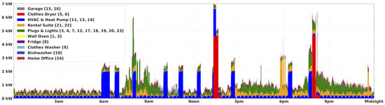
Figure 1. Plot of all loads over 24 h on Sunday, 20 March 2016 for House 1.

This dataset has two overall files, all_sites.txt and all_types.txt, and a number of site-specific data files which are described in Table 1. The file all_sites.txt contains summary information on all the monitored sites in the dataset. A house would be considered a monitoring site. As different monitoring sites are added, the type of sites will be defined in the all_types.txt file.

Table 1. Dataset file descriptions.

File Name	Description
all_sites.txt	Summary data for all monitored sites (e.g., houses). See Table 2 for a description of the columns in this file.
all_types.txt	A dictionary that describes the type of sites that were monitored.
<type>?.txt	Metadata for the given <type> of site monitored followed by its ID. For example, a house of ID 1 would have the filename house1.txt. See Table 3 for more details. There is one file for each site.
<type>?_energy_blk?.csv	Energy data recorded at hourly intervals for all sub-meters. See Table 4 for more details. There is one file for each reading block of each site.
<type>?_labels.txt	Descriptions of each sub-meter monitored (the sub-meter number followed by description), one per line. The number corresponds to the sub column in the power and energy data files. (e.g., 1 would be sub1). There is one file for each site.
<type>?_panel.pdf	A diagram of the power panel of each house showing the layout fo the breakers and what breakers where monitored. There is one file for each site.
<type>?_power_blk?.csv	Power data recorded at 1 Hz for all sub-meters. IHD data is also recorded but appears at a lower frequency. See Table 4 for more details. There is one file for each reading block of each site.
<type>?_subs_blk?.csv	Extensive electrical measurements for all sub-meters. See Table 5 for a list of these measurements. There is one file for each reading block of each site.
<type>?_tstat_blk?.csv	HVAC thermostat data recorded at approximately 5 min intervals for each thermostat in a house. Data in these files are highly diverse and depend on the thermostat make/model. To compensate for this, columns in these files are verbosely named. There is one file for each reading block of each site.

Table 2. Column descriptions for the all_sites.txt file.

Column Name	Description
type	The type of site monitored. For example, house would mean residential and could be detached, row, or apartment. Future values could include store, for a store front, industry, for an industrial complex, office, etc. See the all_types.txt file.
id	The house/store/etc. ID number, starting at 1.
power_data	An indicator of whether power and energy data is available (Yes/No). Power data is usually recorded at 1 Hz, whereas energy data is recorded in hourly intervals.
submeters	The number of power sub-meters monitored.
tstat_data	An indicator of whether HVAC thermostat data is available (Yes/No).
block_count	The number of contiguous recorded data blocks for the given house.
timezone	The timezone in which the given house is located.
active	An indicator of whether this house is still under active monitoring (Yes/No). If so, more house data will be added in the future.

Each house has a labels file to describe the loads that each sub-meter monitored accompanied by a panel file to depict the house’s power breaker panel that was sub-metered. Given that these houses are located in Canada, there are larger appliances (e.g., clothes dryers) that have two lines (or sub-meters) for monitoring (L1 and L2) a single appliance. To combine these two lines into one appliance reading, simply add the L1 sub-meter and the L2 sub-meter readings together.

Each site can have one or more contiguous sampling blocks (blk). If there is a significant period of time where the capture of a house stops and then starts, we break that up into two blocks. This helps researchers and data scientists with algorithm testing where contiguous streams of time-series data are necessary. This data, along with other meta data (see Table 3), is stored in the “<type>?.txt” file. For House 1, this file would be house1.txt. Each block has the following files associated with it (see Table 1). The power and energy files contain all real power measurements from mains and sub-meters (good for testing NILM). The subs files contain 11 electrical measurements for each sub-meter. When the HVAC system has electric heating and cooling, we include a tstat file that contains data from the house’s thermostat.

Table 3. Metadata description files for each house.

Column Name	Description
<Site Type> ID	The ID number of the monitored site. If the site is a house then the row heading will read House ID.
Type Details	A description of the monitoring site.
Location	The city, province, and country in which the monitored site is located.
Local Timezone	The local timezone of the monitored site.
Year Built	The year that the building was built.
Year Last Reno	The last year that any major renovations were made.
EnerGuide	If the building has an EnerGuide rating, when it was given.
HVAC Type	A description of the type of HVAC system installed at the monitored site.
Lighting	A description of the type of lighting used at the monitored site.
Thermostat(s)	A list of HVAC thermostats on site, including their make and model.
IHD Device	The model of Rainforest Automation in-home display used to record smart meter data.
Sub-meter Equip	The model of equipment used to monitor power panel breakers.
Sub-meter Count	The number of sub-meters/breakers monitored.
Sub-meter Mains	The aggregated total power/energy. If value calc is given, then mains is calculated by a summation of all sub-meters. Else, listed are sub-meters that monitored the mains. For example, sub1, sub2 would mean that sub-meter 1 (on L1) + sub-meter 2 (on L2) monitored the mains.
Active Site	An indicator of whether the site is still being monitored. If so, more data will be added to the dataset for this site in the future.
Other DOI/URL	A URL for a website with more information about the site. There may be other publications.
Floors	The number of floors at the site. This is followed by one line per floor. The name of the floor, the area/size of the floor, and the number of occupants that usually inhabit that floor.
Occupant Notes	The number of special occupancy notes.
Sampling Blocks	The number of contiguous monitoring blocks.
Missing Data	The number of places where missing data has occurred.

3. Methods

When designing the data capture system for RAE, we prioritized the need for accuracy and reliability. Hence, we chose commercial-grade metering equipment. We chose to use the Rainforest Automation EMU2 in-home display1 to capture smart meter data. See Table 4 (column name ihd) for the data we captured from the EMU2. The EMU2 reads data from a ZigBee-enabled smart meter at roughly 15 s intervals.

Table 4. Column descriptions for power and energy data files.

Column Name	Description
unix_ts	The Unix timestamp is UTC. Note that the local timezone is noted in the house metadata file and all_houses.txt file.
ihd	The value reported by the IHD and the given timestamp. An empty (or null) value would means there was no reading given at that timestamp.
mains	Values in this column are calculated either by a summation of all the sub-meters or by the summation of one or two specific sub-meters used to monitor the mains. This is described in the metadata file for each house.
sub?	Each sub-meter will have a column from 1 to the number of sub-meters (e.g., sub1, sub2, …, sub24).

To capture sub-meter data, we chose a Class 1 branch circuit power meter from DENT, the PowerScout 242. We had prior experience with using the DENT PowerScout 18 m. See Table 5 for the data we captured from the PowerScout 24. The PowerScout 24 can monitor up to 24 circuits at a rate of 1 Hz.

Table 5. Measurements captured by the DENT PowerScout 24.

Column	Description	Units
0	Unix Timestamp (since Epoch)	s
1	Sub-meter ID (sub)	$number$
2	Voltage (V)	V
3	Frequency (f)	Hz
4	Current (I)	A
5	Displacement Power Factor (dPF)	$ratio$
6	Apparent Power Factor (aPF)	$ratio$
7	Real Power (P)	W
8	Reactive Power (Q)	VAR
9	Apparent Power (S)	VA
10	Real Energy (Pt)	Wh
11	Reactive Energy (Qt)	VARh
12	Apparent Energy (St)	VAh

Thermostat data was collected from the EcoBee3 thermostat3 at 5 min intervals (a product limitation). Data includes set points, operation mode (heat/cool and stage), outdoor temperature and wind speed, and indoor humidity. Indoor temperature and motion is reported from the thermostat and three remote sensors (located in the living room, the basement rec room, and the master bedroom).

The hardware setup used to capture data for RAE is depicted in Figure 2, and we have released (as open source) the code4 used to capture, store, and convert the raw data. This setup is minimal and will allow us to easily install this equipment in a different house to capture data and add it to the RAE dataset.

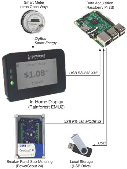
Figure 2. Diagram of the data capturing hardware/setup.

Data that is missing will be represented by a timestamp and one or more null data-points. For comma-separated value (CSV) files, this would mean no data between commas. For example, “1457282030,,,,4.582,38193.4” would mean that three readings are missing.

4. Usage Notes

4.1. House 1 Energy Consumption Analysis

The three highest consumers of energy in House 1 were the HVAC & Heat Pump (570 kWh), Plugs & Lights (531 kWh), and Rental Suite (430 kWh), as shown in Figure 3. Over the 72-day capture period, the smart meter reported a total energy consumption of 1982 kWh. A total of 1971 kWh was found when each of the 24 sub-meters real energy accumulator is summed up. There is an 11 kWh discrepancy due to the rounding errors in each sub-meter accumulator as each sub-meter reports only whole-Watt measurements. Additionally, the smart meter from the utility is a Class 1 m, whereas the sub-meters are Class 0.5. This means there is a higher measurement error in the readings from the smart meter.

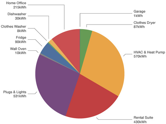
Figure 3. Percentages of energy consumed (in kWh) over the 72-day period for a total of 1971 kWh.

4.2. House 2 Energy Consumption Analysis

House 2 is a smaller (26.1 m${}^2$ less space) and more energy-efficient house than House 1. Plugs & Lights (242.5 kWh) were the highest consumers of energy, as shown in Figure 4. Over the 59-day capture period, the smart meter reported a total energy consumption of 478 kWh. A total of 497 kWh is found when each of the 21 sub-meters real energy accumulator is summed up. There is a 19 kWh discrepancy which is due to the same issues mentioned in the previous sub-section.

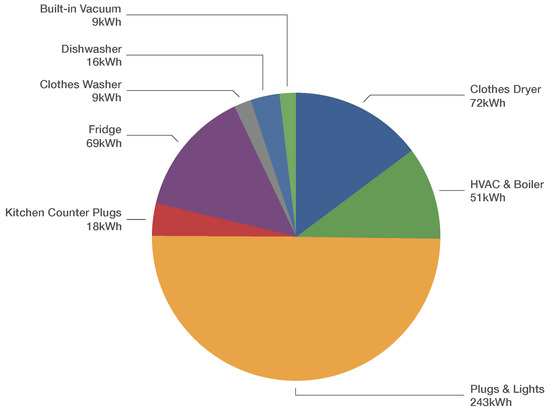
Figure 4. Percentages of energy consumed (in kWh) over the 59-day period for a total of 478 kWh.

4.3. NILM Example

We wanted to use the RAE dataset to test the accuracy of the NILM algorithm. For this, we used the SparseNILM algorithm [3]. SparseNILM uses a variant of the Viterbi algorithm to find the most likely set of appliances that are ON in each time period (as well as their power level) and a rate matching the dataset used — in this case, 1 Hz. We ran our test on a MacBook Pro (13-inch, Late 2016) having a 3.3 GHz Intel Core i7 processor with a 16 GB memory.

First, we removed the rental suite sub-panel power data so that we could test for a single occupancy home. Second, we picked six high-consuming loads (clothes dryer, furnace, heat pump, oven, fridge, and dishwasher) to disaggregate. Third, we trained the algorithm using data from the first block file (nine days). This resulted in the creation of a 2000-state hidden Markov model (HMM) that modeled all six loads. The training phase (consisting of one iteration) took 58 s to complete.

Next, we tested the accuracy of our HMM by having it disaggregate the data from the second block file (63 days). Testing took 46 min to complete, disaggregating 5.4 million samples with an average disaggregation time of 330 $\mathsf{\mu }$s per sample,. We report overall accuracy results in Table 6. Figure 5 shows the accuracy results of each appliance/load that was disaggregated. Our experiment yielded an accuracy of over 80% and very low error results.

Table 6. Overall accuracy results of our NILM test.

Accuracy Metric	Score
Precision	87.86%
Recall	85.01%
F-score	86.41%
Finite-State F-score (FS-fscore) [10]	80.47%
Normalized Disaggregation Error (NDE) [11]	0.71%
Root-Mean-Square Error (RMSE)	62.14

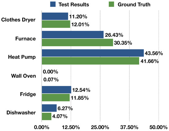
Figure 5. Appliance/load-specific accuracy results (in percentages of total desegregated, not of the total house).

References

- Hadzic, F.; Tan, H.; Dillon, T.S. Mining of Data with Complex Structures; Springer: Berlin, Germany, 2011; Volume 333. [Google Scholar]
- Hart, G.W. Nonintrusive appliance load monitoring. Proc. IEEE 1992, 80, 1870–1891. [Google Scholar] [CrossRef]
- Makonin, S.; Popowich, F.; Bajić, I.V.; Gill, B.; Bartram, L. Exploiting HMM Sparsity to Perform Online Real-Time Nonintrusive Load Monitoring. IEEE Trans. Smart Grid 2016, 7, 2575–2585. [Google Scholar] [CrossRef]
- Makonin, S.; Popowich, F.; Bartram, L.; Gill, B.; Bajić, I.V. AMPds: A public dataset for load disaggregation and eco-feedback research. In Proceedings of the 2013 IEEE Electrical Power Energy Conference, Halifax, NS, Canada, 21–23 August 2013. [Google Scholar]
- Makonin, S.; Ellert, B.; Bajić, I.; Popowich, F. Electricity, water, and natural gas consumption of a residential house in Canada from 2012 to 2014. Sci. Data 2016, 3, 160037. [Google Scholar] [CrossRef] [PubMed]
- Kolter, J.Z.; Johnson, M.J. REDD: A public data set for energy disaggregation research. In Proceedings of the Workshop on Data Mining Applications in Sustainability (SIGKDD), San Diego, CA, USA, 21 August 2011; pp. 59–62. [Google Scholar]
- Kelly, J.; Knottenbelt, W. The UK-DALE dataset, domestic appliance-level electricity demand and whole-house demand from five UK homes. Sci. Data 2015, 2, 150007. [Google Scholar] [CrossRef] [PubMed]
- Anderson, K.; Ocneanu, A.F.; Benitez, D.; Carlson, D.; Rowe, A.; Berges, M. BLUED: A fully labeled public dataset for event-based non-intrusive load monitoring research. In Proceedings of the 2nd Workshop on Data Mining Applications in Sustainability (SustKDD), San Diego, CA, USA, 21 August 2011. [Google Scholar]
- Picon, T.; Meziane, M.N.; Ravier, P.; Lamarque, G.; Novello, C.; Bunetel, J.C.L.; Raingeaud, Y. COOLL: Controlled On/Off Loads Library, a Public Dataset of High-Sampled Electrical Signals for Appliance Identification. arXiv, 2016; arXiv:preprint/1611.05803. [Google Scholar]
- Makonin, S.; Popowich, F. Nonintrusive load monitoring (NILM) performance evaluation. Energy Effic. 2014, 8, 809–814. [Google Scholar] [CrossRef]
- Parson, O.; Ghosh, S.; Weal, M.; Rogers, A. Non-Intrusive Load Monitoring Using Prior Models of General Appliance Types. In Proceedings of the Twenty-Sixth AAAI Conference on Artificial Intelligence (AAAI’12), Toronto, ON, Canada, 22–26 July 2012. [Google Scholar]