The Effect of Quantum Noise on Multipartite Entanglement from a Cascaded Parametric Amplifier

Abstract

The tripartite entanglement generated from a cascaded parametric amplifier is always present in the whole gain region in the ideal condition. However, in practical applications, the quantum entanglement is very fragile and easily deteriorated by quantum noise from interactions with external environments, e.g., the avoidable attenuation and amplification operations may lead to some degradation effects on the quantum entanglement. Therefore, in this work, bipartite entanglement for the three pairs and tripartite entanglement in this cascaded parametric amplifier under the circumstances of attenuation and amplification operations are analyzed by using positivity under partial transposition criterion. The results show that tripartite entanglement is robust to the deterioration effects from the attenuation and amplification operations rather than bipartite entanglement. Our results may find some practical applications of multipartite quantum entanglement in quantum secure communications.

1. Introduction

Attenuation and amplification operations can both introduce extra noise, which can inevitably affect the physical properties of the different systems. For example, in the classical regime it has been found that for an ideal amplification process, the noise figure (NF) of a transmitted light beam never exceeds a factor of two, while for an attenuation process, there is no limit as to how large the NF can become [1]. More importantly, in the quantum regime, the effects of attenuation and amplification on the exact solution to the master equation of a nonlinear oscillator are presented, and it is shown that amplification destroys quantum coherence more rapidly than attenuation does [2]; the behavior of the non-Gaussian state of light under the actions of probabilistic noiseless amplification and attenuation is examined, and it is found that the mean-field amplitude may decrease (increase) in the process of noiseless amplification (attenuation) [3], and the authors analyze the general laws of continuous-variable (CV) entanglement dynamics during the deterministic attenuation and amplification of the physical signal carrying the entanglement [4]. As discussed above, the attenuation and amplification operations can largely influence the behaviors of the physical systems by means of the different ways.

The parametric amplifier, for example, the four-wave mixing (FWM) process, acts as an effective quantum device to generate bipartite entanglement [5,6,7,8,9] in the CV domain. Recently, it has been reported that by cascading the two FWM processes, the tunable delay of the Einstein-Podolsky-Rosen entangled state [10], the low-noise amplification of an entangled state [11], SU(1,1) interferometer [12,13], and quantum mutual information [14] have been experimentally realized. In 2014, it has been theoretically proposed and experimentally demonstrated that a cascaded FWM system can be used to generate multiple quantum correlated beams based on the atomic ensemble [15]. After that, tripartite entanglement generated from this cascaded parametric amplifier has been theoretically proved to be present in the whole gain region in the ideal condition [16]. However, in practical applications, quantum entanglement is very fragile and easily deteriorated by the quantum noise from the interaction with external environment, e.g., unavoidable attenuation and amplification operations may lead to some deterioration effects to quantum entanglement [17]. It should be emphasized that in Ref. [18] the optical losses introduced by the attenuation operation as the inevitable experimental imperfections are used to consider their deterioration effect on the entanglement of subsystems and multipartite entanglement generated by cascaded FWM processes. In the present work the deterioration effect introduced by the amplification operation is also considered. Therefore, here bipartite entanglement for the three pairs and tripartite entanglement in this cascaded parametric amplifier under the circumstances of attenuation and amplification operations are both analyzed by using positivity under partial transposition (PPT) criterion [19,20,21,22]. The results show that tripartite entanglement is robust to the deterioration effects from the attenuation and amplification operations rather than bipartite entanglement.

This work is organized as follows. In Section 2, we describe the physical system of the cascaded FWM processes under the cases of the attenuation and amplification operations. In Section 3, the effect of the detector imperfections on bipartite entanglement and tripartite entanglement is characterized by using PPT criterion. In Section 4, the effects of the attenuation and amplification operations are also analyzed. In Section 5, we give a brief summary of this work.

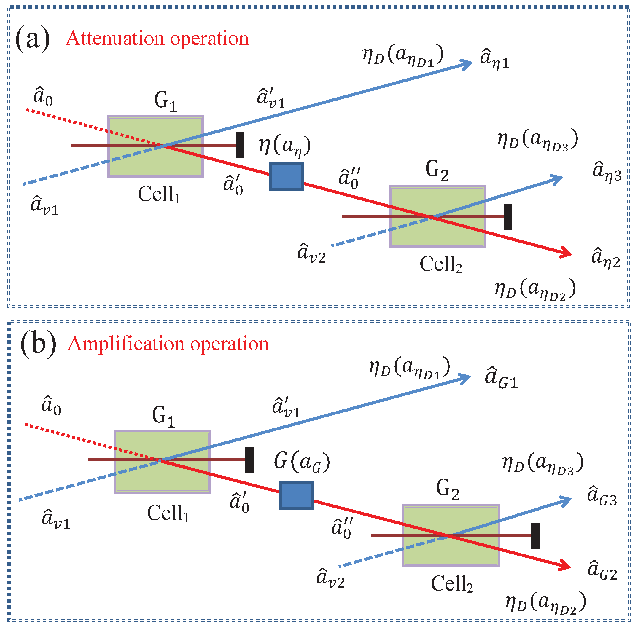
2. Cascaded FWM Processes under the Cases of the Attenuation and Amplification Operations

Cascaded FWM processes under the cases of attenuation and amplification operations are depicted in Figure 1. As depicted in Figure 1a, an intense pump beam and a much weaker signal mode are crossed in the center of cell${}_1$ with a small angle; then, the signal mode is amplified and a new idler mode is generated on the other side of the pump beam at the same time. After that, the signal mode from the first FWM process (cell${}_1$) as the seed is again seeded into the second FWM process (cell${}_2$). ${\widehat{a}}_{\eta 1}$, ${\widehat{a}}_{\eta 2}$, and ${\widehat{a}}_{\eta 3}$ are three newly-generated modes in the output stage of the cascaded processes. The detection efficiencies for the three modes ${\widehat{a}}_{\eta 1}$, ${\widehat{a}}_{\eta 2}$, and ${\widehat{a}}_{\eta 3}$ are assumed to be the same for the sake of simplicity. More importantly, the attenuation operation is acted upon by $\eta$ in Figure 1a. To analyze the effect of the attenuation operation on bipartite entanglement for the three pairs and tripartite entanglement, the input–output relation in Figure 1a can be written as

$$\begin{array}{ccc}\hfill {\widehat{a}}_{\eta 1}& =& \sqrt{{\eta }_D}{\widehat{a}}_{v1}^{{}^{\prime }}+\sqrt{1-{\eta }_D}{\widehat{a}}_{\eta D1}\hfill \\ & =& \sqrt{{\eta }_D}[\sqrt{G_1}{\widehat{a}}_{v1}+\sqrt{g_1}{\widehat{a}}_0^{†}]+\sqrt{1-{\eta }_D}{\widehat{a}}_{\eta D1}\hfill \\ & =& \sqrt{G_1{\eta }_D}{\widehat{a}}_{v1}+\sqrt{g_1{\eta }_D}{\widehat{a}}_0^{†}+\sqrt{1-{\eta }_D}{\widehat{a}}_{\eta D1},\hfill \end{array}$$

(1)

$$\begin{array}{ccc}\hfill {\widehat{a}}_{\eta 2}& =& \sqrt{{\eta }_D}[\sqrt{G_2}{\widehat{a}}_0^{{}^{″}}+\sqrt{g_2}{\widehat{a}}_{v2}^{†}]+\sqrt{1-{\eta }_D}{\widehat{a}}_{\eta D2}\hfill \\ & =& \sqrt{G_2{\eta }_D}{\widehat{a}}_0^{{}^{″}}+\sqrt{g_2{\eta }_D}{\widehat{a}}_{v2}^{†}+\sqrt{1-{\eta }_D}{\widehat{a}}_{\eta D2}\hfill \\ & =& \sqrt{G_2{\eta }_D}[\sqrt{\eta }{\widehat{a}}_0^{{}^{\prime }}+\sqrt{1-\eta }{\widehat{a}}_{\eta }]+\sqrt{g_2{\eta }_D}{\widehat{a}}_{v2}^{†}+\sqrt{1-{\eta }_D}{\widehat{a}}_{\eta D2}\hfill \\ & =& \sqrt{G_2{\eta }_D\eta }{\widehat{a}}_0^{{}^{\prime }}+\sqrt{G_2{\eta }_D(1-\eta )}{\widehat{a}}_{\eta }+\sqrt{g_2{\eta }_D}{\widehat{a}}_{v2}^{†}+\sqrt{1-{\eta }_D}{\widehat{a}}_{\eta D2}\hfill \\ & =& \sqrt{G_2{\eta }_D\eta }[\sqrt{G_1}{\widehat{a}}_0+\sqrt{g_1}{\widehat{a}}_{v1}^{†}]+\sqrt{G_2{\eta }_D(1-\eta )}{\widehat{a}}_{\eta }\hfill \\ & & +\sqrt{g_2{\eta }_D}{\widehat{a}}_{v2}^{†}+\sqrt{1-{\eta }_D}{\widehat{a}}_{\eta D2}\hfill \\ & =& \sqrt{G_1{G}_2\eta {\eta }_D}{\widehat{a}}_0+\sqrt{G_2{g}_1\eta {\eta }_D}{\widehat{a}}_{v1}^{†}+\sqrt{G_2{\eta }_D(1-\eta )}{\widehat{a}}_{\eta }\hfill \\ & & +\sqrt{g_2{\eta }_D}{\widehat{a}}_{v2}^{†}+\sqrt{1-{\eta }_D}{\widehat{a}}_{{\eta }_{D2}},\hfill \end{array}$$

(2)

$$\begin{array}{ccc}\hfill {\widehat{a}}_{\eta 3}& =& \sqrt{{\eta }_D}[\sqrt{G_2}{\widehat{a}}_{v2}+\sqrt{g_2}{\widehat{a}}_0^{{}^{″}†}]+\sqrt{1-{\eta }_D}{\widehat{a}}_{\eta D3}\hfill \\ & =& \sqrt{G_2{\eta }_D}{\widehat{a}}_{v2}+\sqrt{g_2{\eta }_D}{\widehat{a}}_0^{{}^{″}†}+\sqrt{1-{\eta }_D}{\widehat{a}}_{\eta D3}\hfill \\ & =& \sqrt{G_2{\eta }_D}{\widehat{a}}_{v2}+\sqrt{g_2{\eta }_D}[\sqrt{\eta }{\widehat{a}}_0^{{}^{\prime }†}+\sqrt{1-\eta }{\widehat{a}}_{\eta }^{†}]+\sqrt{1-{\eta }_D}{\widehat{a}}_{\eta D3}\hfill \\ & =& \sqrt{G_2{\eta }_D}{\widehat{a}}_{v2}+\sqrt{g_2{\eta }_D\eta }[\sqrt{G_1}{\widehat{a}}_0^{†}+\sqrt{g_1}{\widehat{a}}_{v1}]+\sqrt{g_2{\eta }_D(1-\eta )}{\widehat{a}}_{\eta }^{†}+\sqrt{1-{\eta }_D}{\widehat{a}}_{\eta D3}\hfill \\ & =& \sqrt{G_2{\eta }_D}{\widehat{a}}_{v2}+\sqrt{G_1{g}_2{\eta }_D\eta }{\widehat{a}}_0^{†}+\sqrt{g_1{g}_2{\eta }_D\eta }{\widehat{a}}_{v1}+\sqrt{g_2{\eta }_D(1-\eta )}{\widehat{a}}_{\eta }^{†}\hfill \\ & & +\sqrt{1-{\eta }_D}{\widehat{a}}_{\eta D3},\hfill \end{array}$$

(3)

where G_j (j = 1, 2) is the power gain in the FWM process and G_j $-g_j$ = 1. Equations (1)–(3) can be rewritten in the form of the quadrature operators as follows:

$$\begin{array}{ccc}\hfill {\widehat{X}}_{\eta 1}& =& {\widehat{a}}_{\eta 1}+{\widehat{a}}_{\eta 1}^{†}=\sqrt{G_1{\eta }_D}{\widehat{X}}_{v1}+\sqrt{g_1{\eta }_D}{\widehat{X}}_0+\sqrt{1-{\eta }_D}{\widehat{X}}_{{\eta }_{D1}},\hfill \end{array}$$

(4)

$$\begin{array}{ccc}\hfill {\widehat{X}}_{\eta 2}& =& {\widehat{a}}_{\eta 2}+{\widehat{a}}_{\eta 2}^{†}=\sqrt{G_1{G}_2\eta {\eta }_D}{\widehat{X}}_0+\sqrt{G_2{g}_1\eta {\eta }_D}{\widehat{X}}_{v1}+\sqrt{G_2{\eta }_D(1-\eta )}{\widehat{X}}_{\eta }\hfill \\ & & +\sqrt{g_2{\eta }_D}{\widehat{X}}_{v2}+\sqrt{1-{\eta }_D}{\widehat{X}}_{{\eta }_{D2}},\hfill \end{array}$$

(5)

$$\begin{array}{ccc}\hfill {\widehat{X}}_{\eta 3}& =& {\widehat{a}}_{\eta 3}+{\widehat{a}}_{\eta 3}^{†}=\sqrt{G_2{\eta }_D}{\widehat{X}}_{v2}+\sqrt{G_1{g}_2\eta {\eta }_D}{\widehat{X}}_0+\sqrt{g_1{g}_2\eta {\eta }_D}{\widehat{X}}_{v1}\hfill \\ & & +\sqrt{g_2(1-\eta ){\eta }_D}{\widehat{X}}_{\eta }+\sqrt{1-{\eta }_D}{\widehat{X}}_{{\eta }_{D3}},\hfill \end{array}$$

(6)

and

$$\begin{array}{ccc}\hfill {\widehat{Y}}_{\eta 1}& =& -i({\widehat{a}}_{\eta 1}-{\widehat{a}}_{\eta 1}^{†})=\sqrt{G_1{\eta }_D}{\widehat{Y}}_{v1}-\sqrt{g_1{\eta }_D}{\widehat{Y}}_0+\sqrt{1-{\eta }_D}{\widehat{Y}}_{{\eta }_{D1}},\hfill \end{array}$$

(7)

$$\begin{array}{ccc}\hfill {\widehat{Y}}_{\eta 2}& =& -i({\widehat{a}}_{\eta 2}-{\widehat{a}}_{\eta 2}^{†})=\sqrt{G_1{G}_2\eta {\eta }_D}{\widehat{Y}}_0-\sqrt{G_2{g}_1\eta {\eta }_D}{\widehat{Y}}_{v1}+\sqrt{G_2{\eta }_D(1-\eta )}{\widehat{Y}}_{\eta }\hfill \\ & & -\sqrt{g_2{\eta }_D}{\widehat{Y}}_{v2}+\sqrt{1-{\eta }_D}{\widehat{Y}}_{{\eta }_{D2}},\hfill \end{array}$$

(8)

$$\begin{array}{ccc}\hfill {\widehat{Y}}_{\eta 3}& =& -i({\widehat{a}}_{\eta 3}-{\widehat{a}}_{\eta 3}^{†})=\sqrt{G_2{\eta }_D}{\widehat{Y}}_{v2}-\sqrt{G_1{g}_2\eta {\eta }_D}{\widehat{Y}}_0+\sqrt{g_1{g}_2\eta {\eta }_D}{\widehat{Y}}_{v1}\hfill \\ & & -\sqrt{g_2(1-\eta ){\eta }_D}{\widehat{Y}}_{\eta }+\sqrt{1-{\eta }_D}{\widehat{Y}}_{{\eta }_{D3}},\hfill \end{array}$$

(9)

where $\widehat{X}$ and $\widehat{Y}$ represent the amplitude and phase quadratures, respectively, and have the commutation relation $[\widehat{X},\widehat{Y}]=2i$. From the above expressions for the quadrature operators, the variances and covariances of amplitude and phase quadratures can be obtained to construct covariance matrix (CM${}_{\eta 123}$). $\langle {\widehat{X}}_m^2\rangle$ denotes the amplitude quadrature variance due to the zero mean value of $\langle {\widehat{X}}_m\rangle$. Similarly, for the covariance, we use the notation $\langle {\widehat{X}}_m{\widehat{X}}_n\rangle$ and for the case where m = n it will reduce to the usual variance, $\langle {\widehat{X}}_m^2\rangle$. Therefore, the variances and covariances of tripartite entanglement under the case of attenuation operation can be expressed as

$$\begin{array}{ccc}\hfill 〈{\widehat{X}}_{\eta 1}^2〉& =& 〈{\widehat{Y}}_{\eta 1}^2〉=(2G_1-1){\eta }_D+(1-{\eta }_D),\hfill \end{array}$$

(10)

$$\begin{array}{ccc}\hfill 〈{\widehat{X}}_{\eta 2}^2〉& =& 〈{\widehat{Y}}_{\eta 2}^2〉=2G_2\eta {\eta }_D(G_1-1)+(2G_2-1){\eta }_D+(1-{\eta }_D),\hfill \end{array}$$

(11)

$$\begin{array}{ccc}\hfill 〈{\widehat{X}}_{\eta 3}^2〉& =& 〈{\widehat{Y}}_{\eta 3}^2〉=2\eta {\eta }_D(G_1-1)(G_2-1)+(2G_2-1){\eta }_D\hfill \\ & & +(1-{\eta }_D),\hfill \end{array}$$

(12)

$$\begin{array}{ccc}\hfill 〈{\widehat{X}}_{\eta 1}{\widehat{X}}_{\eta 2}〉& =& -〈{\widehat{Y}}_{\eta 1}{\widehat{Y}}_{\eta 2}〉=2{\eta }_D\sqrt{G_1(G_1-1)G_2\eta },\hfill \end{array}$$

(13)

$$\begin{array}{ccc}\hfill 〈{\widehat{X}}_{\eta 1}{\widehat{X}}_{\eta 3}〉& =& 〈{\widehat{Y}}_{\eta 1}{\widehat{Y}}_{\eta 3}〉=2{\eta }_D\sqrt{G_1(G_1-1)(G_2-1)\eta },\hfill \end{array}$$

(14)

$$\begin{array}{ccc}\hfill 〈{\widehat{X}}_{\eta 2}{\widehat{X}}_{\eta 3}〉& =& -〈{\widehat{Y}}_{\eta 2}{\widehat{Y}}_{\eta 3}〉=2\eta {\eta }_D(G_1-1)\sqrt{G_2(G_2-1)}\hfill \\ & & +2{\eta }_D\sqrt{G_2(G_2-1)}.\hfill \end{array}$$

(15)

Equations (10)–(15) contain all of the information about tripartite entanglement under the case of attenuation operation when attenuation operation is switched to amplification operation. Similarly, the input–output relation of tripartite entanglement under the case of amplification operation in Figure 1b can be given by

$$\begin{array}{ccc}\hfill {\widehat{a}}_{G1}& =& \sqrt{G_1{\eta }_D}{\widehat{a}}_{v1}+\sqrt{g_1{\eta }_D}{\widehat{a}}_0^{†}+\sqrt{1-{\eta }_D}{\widehat{a}}_{{\eta }_{D1}},\hfill \end{array}$$

(16)

$$\begin{array}{ccc}\hfill {\widehat{a}}_{G2}& =& \sqrt{G_1{G}_{2}G{\eta }_D}{\widehat{a}}_0+\sqrt{G_2{g}_{1}G{\eta }_D}{\widehat{a}}_{v1}^{†}+\sqrt{G_2{\eta }_D(G-1)}{\widehat{a}}_G^{†}\hfill \\ & & +\sqrt{g_2{\eta }_D}{\widehat{a}}_{v2}^{†}+\sqrt{1-{\eta }_D}{\widehat{a}}_{{\eta }_{D2}},\hfill \end{array}$$

(17)

$$\begin{array}{ccc}\hfill {\widehat{a}}_{G3}& =& \sqrt{G_2{\eta }_D}{\widehat{a}}_{v2}+\sqrt{G_1(G_2-1)G{\eta }_D}{\widehat{a}}_0^{†}+\sqrt{G(G_1-1)(G_2-1){\eta }_D}{\widehat{a}}_{v1}\hfill \\ & & +\sqrt{g_2(G-1){\eta }_D}{\widehat{a}}_G+\sqrt{1-{\eta }_D}{\widehat{a}}_{{\eta }_{D3}},\hfill \end{array}$$

(18)

similarly, the corresponding quadrature operators of the three modes ${\widehat{a}}_{G1}$, ${\widehat{a}}_{G2}$, and ${\widehat{a}}_{G3}$ can also be written as

$$\begin{array}{ccc}\hfill {\widehat{X}}_{G1}& =& {\widehat{a}}_{G1}+{\widehat{a}}_{G1}^{†}=\sqrt{G_1{\eta }_D}{\widehat{X}}_{v1}+\sqrt{g_1{\eta }_D}{\widehat{X}}_0+\sqrt{1-{\eta }_D}{\widehat{X}}_{{\eta }_{D1}},\hfill \end{array}$$

(19)

$$\begin{array}{ccc}\hfill {\widehat{X}}_{G2}& =& {\widehat{a}}_{G2}+{\widehat{a}}_{G2}^{†}=\sqrt{G_1{G}_{2}G{\eta }_D}{\widehat{X}}_0+\sqrt{G_2{g}_{1}G{\eta }_D}{\widehat{X}}_{v1}+\sqrt{G_2{\eta }_D(G-1)}{\widehat{X}}_G\hfill \\ & & +\sqrt{g_2{\eta }_D}{\widehat{X}}_{v2}+\sqrt{1-{\eta }_D}{\widehat{X}}_{{\eta }_{D2}},\hfill \end{array}$$

(20)

$$\begin{array}{ccc}\hfill {\widehat{X}}_{G3}& =& {\widehat{a}}_{G3}+{\widehat{a}}_{G3}^{†}=\sqrt{G_2{\eta }_D}{\widehat{X}}_{v2}+\sqrt{G_1{g}_{2}G{\eta }_D}{\widehat{X}}_0+\sqrt{g_1{g}_{2}G{\eta }_D}{\widehat{X}}_{v1}\hfill \\ & & +\sqrt{g_2(G-1){\eta }_D}{\widehat{X}}_G+\sqrt{1-{\eta }_D}{\widehat{X}}_{{\eta }_{D3}},\hfill \end{array}$$

(21)

and

$$\begin{array}{ccc}\hfill {\widehat{Y}}_{G1}& =& -i({\widehat{a}}_{G1}-{\widehat{a}}_{G1}^{†})=\sqrt{G_1{\eta }_D}{\widehat{Y}}_{v1}-\sqrt{g_1{\eta }_D}{\widehat{Y}}_0+\sqrt{1-{\eta }_D}{\widehat{Y}}_{{\eta }_{D1}},\hfill \end{array}$$

(22)

$$\begin{array}{ccc}\hfill {\widehat{Y}}_{G2}& =& -i({\widehat{a}}_{G2}-{\widehat{a}}_{G2}^{†})=\sqrt{G_1{G}_{2}G{\eta }_D}{\widehat{Y}}_0-\sqrt{G_2{g}_{1}G{\eta }_D}{\widehat{Y}}_{v1}-\sqrt{G_2{\eta }_D(G-1)}{\widehat{Y}}_G\hfill \\ & & -\sqrt{g_2{\eta }_D}{\widehat{Y}}_{v2}+\sqrt{1-{\eta }_D}{\widehat{Y}}_{{\eta }_{D2}},\hfill \end{array}$$

(23)

$$\begin{array}{ccc}\hfill {\widehat{Y}}_{G3}& =& -i({\widehat{a}}_{G3}-{\widehat{a}}_{G3}^{†})=\sqrt{G_2{\eta }_D}{\widehat{Y}}_{v2}-\sqrt{G_1{g}_{2}G{\eta }_D}{\widehat{Y}}_0+\sqrt{g_1{g}_{2}G{\eta }_D}{\widehat{Y}}_{v1}\hfill \\ & & +\sqrt{g_2(G-1){\eta }_D}{\widehat{Y}}_G+\sqrt{1-{\eta }_D}{\widehat{Y}}_{{\eta }_{D3}},\hfill \end{array}$$

(24)

thus the variances and covariances under the case of amplification operation can also be given by

$$\begin{array}{ccc}\hfill 〈{\widehat{X}}_{G1}^2〉& =& 〈{\widehat{Y}}_{G1}^2〉=(2G_1-1){\eta }_D+(1-{\eta }_D),\hfill \end{array}$$

(25)

$$\begin{array}{ccc}\hfill 〈{\widehat{X}}_{G2}^2〉& =& 〈{\widehat{Y}}_{G2}^2〉=2G_2{G}_{1}G{\eta }_D+(1-2{\eta }_D),\hfill \end{array}$$

(26)

$$\begin{array}{ccc}\hfill 〈{\widehat{X}}_{G3}^2〉& =& 〈{\widehat{Y}}_{G3}^2〉=2G{G}_1(G_2-1){\eta }_D+1,\hfill \end{array}$$

(27)

$$\begin{array}{ccc}\hfill 〈{\widehat{X}}_{G1}{\widehat{X}}_{G2}〉& =& -〈{\widehat{Y}}_{G1}{\widehat{Y}}_{G2}〉=2{\eta }_D\sqrt{G_1(G_1-1)G_{2}G},\hfill \end{array}$$

(28)

$$\begin{array}{ccc}\hfill 〈{\widehat{X}}_{G1}{\widehat{X}}_{G3}〉& =& 〈{\widehat{Y}}_{G1}{\widehat{Y}}_{G3}〉=2{\eta }_D\sqrt{G_1(G_1-1)(G_2-1)G},\hfill \end{array}$$

(29)

$$\begin{array}{ccc}\hfill 〈{\widehat{X}}_{G2}{\widehat{X}}_{G3}〉& =& -〈{\widehat{Y}}_{G2}{\widehat{Y}}_{G3}〉=2G{G}_1{\eta }_D\sqrt{G_2(G_2-1)},\hfill \end{array}$$

(30)

similarly, Equations (25)–(30) contain all of the information about tripartite entanglement under the case of the amplification operation. We will use the above expressions to analyze the entanglement properties of bipartite entanglement for the three pairs and tripartite entanglement under the cases of attenuation and amplification operations because the three modes output from the cascaded FWM system are Gaussian states, and the entanglement properties of Gaussian states can be fully quantified by CM${}_{123}$ (CM${}_{\eta 123}$ and CM${}_{G123}$) using the PPT criterion.

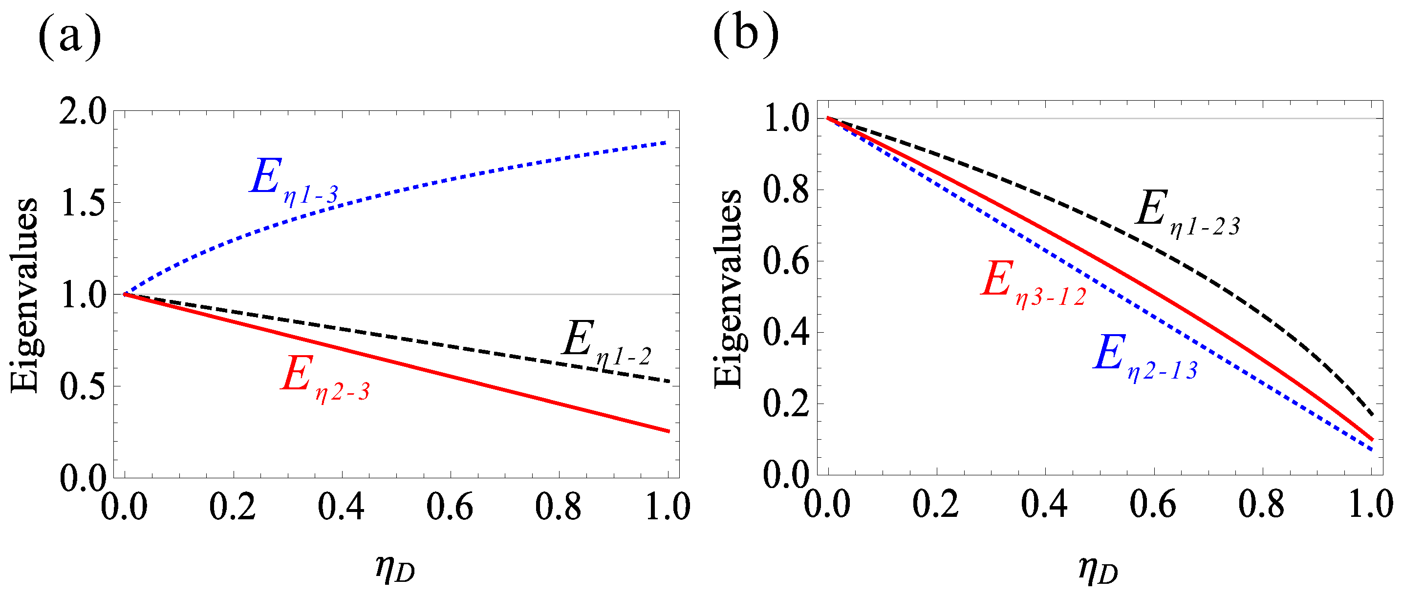
3. The Effect of the Detector Imperfections on Bipartite and Tripartite Entanglement

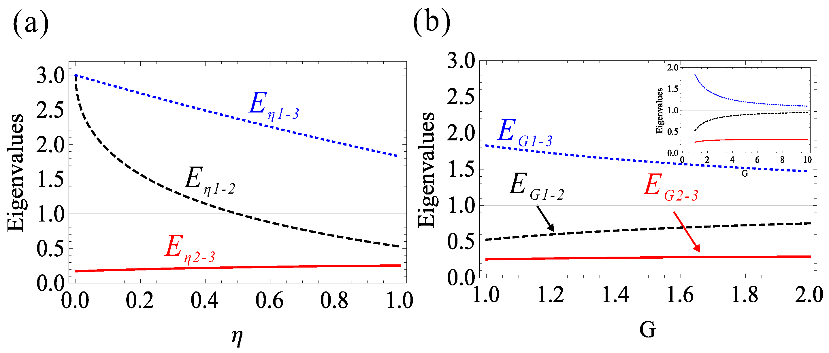
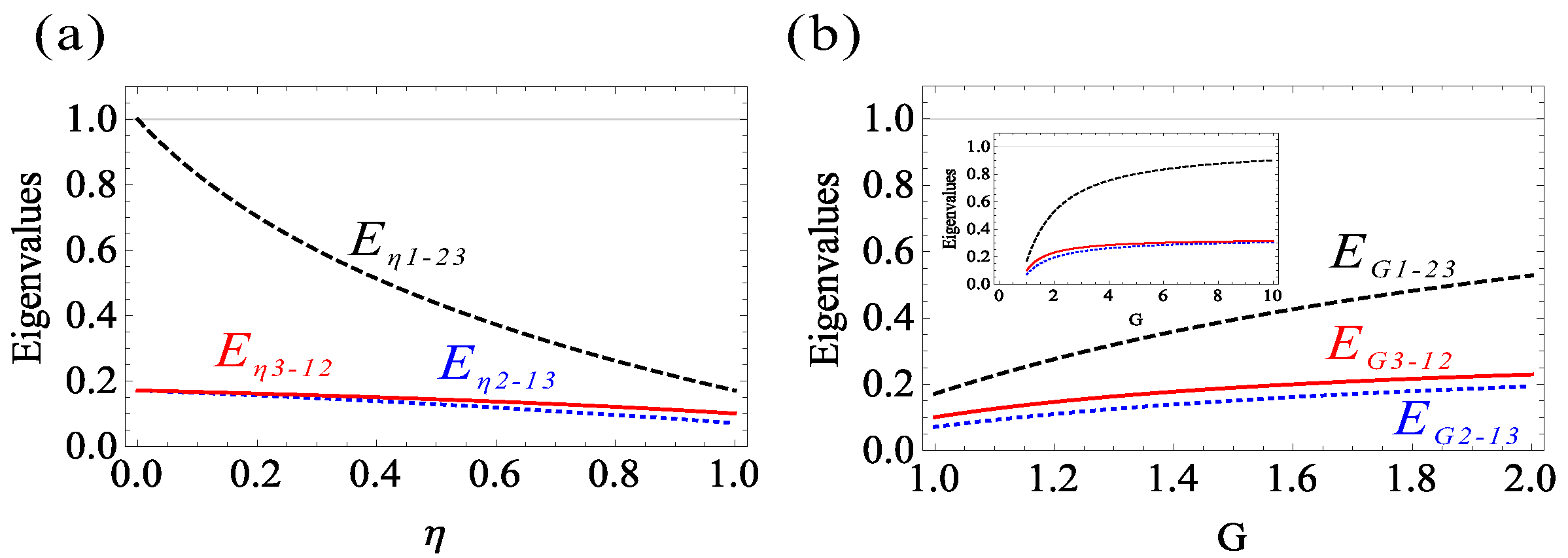
In this section, we will analyze the effect of the detector imperfections ${\eta }_D$ on bipartite and tripartite entanglement. PPT criterion as a sufficient and necessary criterion can be used to quantify the effect of the detector imperfections on quantum entanglement. Firstly, we will focus on bipartite entanglement for the three pairs. For example, only when both of the symplectic eigenvalues of the partially transposed (PT) CM${}_{\eta 12}$ no less than 1 [19,20,21,22], will bipartite entanglement between ${\widehat{a}}_{\eta 1}$ and ${\widehat{a}}_{\eta 2}$ not be present. Following this idea, the smaller symplectic eigenvalue $E_{\eta 1-2}$ can be used to quantify the entanglement between ${\widehat{a}}_{\eta 1}$ and ${\widehat{a}}_{\eta 2}$, i.e., if the smaller symplectic eigenvalue $E_{\eta 1-2}$ is smaller than 1, bipartite entanglement is present between ${\widehat{a}}_{\eta 1}$ and ${\widehat{a}}_{\eta 2}$. Utilizing Equations (10)–(15), we can get the detailed expression of $E_{\eta 1-2}$ as below

$$\begin{array}{ccc}\hfill E_{\eta 1-2}& =& 1+[-2+G_1+(1-\eta +\eta G_1)G_2]{\eta }_D\hfill \\ & & -\sqrt{[G_1^2+2G_1{G}_2(-1-\eta +\eta G_1)+G_2^2{(1-\eta +\eta G_1)}^2]{\eta }_D^2},\hfill \end{array}$$

(31)

the dependence of $E_{\eta 1-2}$ on the detector imperfections ${\eta }_D$ is the black dashed line ($G_1$ = $G_2$ = 2 and $\eta$ = 1) in Figure 2a. The degree of bipartite entanglement between ${\widehat{a}}_{\eta 1}$ and ${\widehat{a}}_{\eta 2}$ increases with the increasing of ${\eta }_D$. We can explain this as follows. Firstly, when ${\eta }_D$ = 1 the two entangled modes ${\widehat{a}}_{\eta 1}$ and ${\widehat{a}}_{\eta 2}$ are fully detected, the symplectic eigenvalue $E_{\eta 1-2}$ is smaller than 1 [16]; secondly, when ${\eta }_D$ = 0, the two detected modes ${\widehat{a}}_{\eta 1}$ and ${\widehat{a}}_{\eta 2}$ are in a vacuum state, respectively, and the entangled state translate into the product state between the two vacuum state (because the correlation term vanishes, i.e., the value of Equation (13) is equal to 0), thus the value of $E_{\eta 1-2}$ is equal to the variance of vacuum state, i.e., $E_{\eta 1-2}$ = 1; thirdly, based on the above arguments, the value of $E_{\eta 1-2}$ decreases with the increasing of ${\eta }_D$. However, it can be shown that the value of $E_{\eta 1-2}$ is always smaller than or equal to 1, meaning that bipartite entanglement between ${\widehat{a}}_{\eta 1}$ and ${\widehat{a}}_{\eta 2}$ is robust to the detector imperfections. Similarly, the smaller symplectic eigenvalue $E_{\eta 1-3}$ of ${\widehat{a}}_{\eta 1}$ and ${\widehat{a}}_{\eta 3}$ is given by

$$\begin{array}{ccc}\hfill E_{\eta 1-3}& =& [-\eta +(-1+\eta )G_2+G_1(1+\eta -\eta G_2)]{\eta }_D+\hfill \\ & & \sqrt{\begin{array}{c}1+2[-2+\eta -(-1+\eta )G_1+G_2+\eta (-1+G_1)G_2]{\eta }_D\\ -4(-1+\eta )(-1+G_1)(-1+G_2){\eta }_D^2+[\eta -(1+\eta )G_1\\ +G_2+\eta (-1+G_1)G_2{]}^2{\eta }_D^2\end{array}},\hfill \end{array}$$

(32)

the dependence of $E_{\eta 1-3}$ on ${\eta }_D$ is the blue dotted line in Figure 2a. Its behavior can be understood as follows. Firstly, when ${\eta }_D$ = 1, the two modes ${\widehat{a}}_{\eta 1}$ and ${\widehat{a}}_{\eta 3}$ with 100% detector efficiency are in thermal state, respectively, because they have been amplified by the independent parametric amplification from different FWM processes, and this leads to the absence of the direct interaction and quantum entanglement. Consequently, the symplectic eigenvalue $E_{\eta 1-3}$ is greater than 1 [16]; secondly, when ${\eta }_D$ = 0, the two modes ${\widehat{a}}_{\eta 1}$ and ${\widehat{a}}_{\eta 3}$ with 0% detector efficiency are in the vacuum state, respectively, and the unentangled state translates into the product state between the two vacuum states (because the correlation term vanishes, i.e., the value of Equation (14) is equal to 0); thus, the value of $E_{\eta 1-3}$ is equal to the variance of the vacuum state, i.e., $E_{\eta 1-3}$=1; finally, according to the above discussions, the value of $E_{\eta 1-3}$ increases with the increasing of ${\eta }_D$ in Figure 2a. However, its value is always greater than or equal to 1, meaning that bipartite entanglement between ${\widehat{a}}_{\eta 1}$ and ${\widehat{a}}_{\eta 3}$ is not robust to the detector imperfections ${\eta }_D$.

In addition, the smaller symplectic eigenvalue $E_{\eta 2-3}$ of ${\widehat{a}}_{\eta 2}$ and ${\widehat{a}}_{\eta 3}$ is given by

$$\begin{array}{ccc}\hfill E_{\eta 2-3}& =& 1+[-2+\eta -2(-1+\eta )G_2+\eta G_1(-1+2G_2)]{\eta }_D\hfill \\ & & -\sqrt{[{\eta }^2{(-1+G_1)}^2-4{(1-\eta +\eta G_1)}^2{G}_2+4{(1-\eta +\eta G_1)}^2{G}_2^2]{\eta }_D^2},\hfill \end{array}$$

(33)

the dependence of $E_{\eta 2-3}$ on ${\eta }_D$ is the red solid line in Figure 2a. Its explanations are analogous to the ones of $E_{\eta 1-2}$ and $E_{\eta 1-3}$. Its value is always smaller than or equal to 1, meaning that bipartite entanglement between ${\widehat{a}}_{\eta 2}$ and ${\widehat{a}}_{\eta 3}$ is also robust to the detector imperfections.

Secondly, the PPT criterion can also be applied to quantify the effect of quantum noise on tripartite entanglement due to PPT criterion as a sufficient and necessary criterion for all 1 × N decompositions of Gaussian states, where N + 1 is the total number of the entangled modes. For the tripartite entanglement condition, the three possible 1 × 2 partitions have to be tested. All of the partitions of the tripartite entangled state are robust to the detector imperfections when the smallest symplectic eigenvalue for each of the three PT CMs is smaller than 1, i.e., tripartite entanglement is robust to the detector imperfections. When PT operation is applied to the modes ${\widehat{a}}_{\eta 1}$, ${\widehat{a}}_{\eta 2}$, and ${\widehat{a}}_{\eta 3}$, the corresponding smallest symplectic eigenvalues are $E_{\eta 1-23}$, $E_{\eta 2-13}$, and $E_{\eta 3-12}$, respectively. The detailed expressions of $E_{\eta 1-23}$, $E_{\eta 2-13}$, and $E_{\eta 3-12}$ are not listed here due to their complexity. However, the results are depicted in Figure 2b; the values of $E_{\eta 1-23}$ (black dashed line), $E_{\eta 2-13}$ (blue dotted line), and $E_{\eta 3-12}$ (red solid line) in Figure 2b are all smaller than or equal to 1, meaning that the three 1 × 2 partitions are robust to the detector imperfections, i.e., the tripartite entanglement is robust to the detector imperfections.

Finally, as the above discussed, bipartite entanglement for the two pairs is not robust to the detector imperfections, while tripartite entanglement is robust to the detector imperfections; this is because bipartite entanglement is the result of the decoherence effect of tripartite entanglement, e.g., bipartite entanglement between ${\widehat{a}}_{\eta 1}$ and ${\widehat{a}}_{\eta 3}$ can be obtained by tracing the mode ${\widehat{a}}_{\eta 2}$ in tripartite entanglement. Therefore, tripartite entanglement containing more entanglement resources is more robust.

4. The Effect of Attenuation Operation $\eta$ and Amplification Operation G on Bipartite and Tripartite Entanglement

After the effect of detector imperfections on bipartite entanglement for the three pairs and tripartite entanglement is analyzed, their robustness degree to attenuation operation $\eta$ and amplification operation G will be investigated in this section. Firstly, we will consider the condition of bipartite entanglement using PPT criterion. The dependence of $E_{\eta 1-2}$ (black dashed line), $E_{\eta 1-3}$ (blue dotted line), and $E_{\eta 2-3}$ (red solid line) on attenuation operation $\eta$ with $G_1$ = $G_2$ = 2 and ${\eta }_D$ = 1 is depicted in Figure 3a. As depicted in Figure 3a, the value of $E_{\eta 1-2}$ decreases with the increasing of $\eta$ and is not always smaller than 1; thus, bipartite entanglement between ${\widehat{a}}_{\eta 1}$ and ${\widehat{a}}_{\eta 2}$ is not always robust to attenuation operation. These phenomena can be understood as follows. When $\eta$ = 1, the two modes ${\widehat{a}}_{\eta 1}$ and ${\widehat{a}}_{\eta 2}$ are in entangled state and the value of $E_{\eta 1-2}$ is smaller than 1 [16]; when $\eta$ = 0, the entangled state between ${\widehat{a}}_{\eta 1}$ and ${\widehat{a}}_{\eta 2}$ translates into the product state between the two thermal states (the value of Equation (13) is equal to 0), so the value of $E_{\eta 1-2}$ is equal to the smaller variance between ${\widehat{a}}_{\eta 1}$ (2$G_1$–1 > 1 for any $G_1$ > 1 in terms of $\eta$ = 0 and ${\eta }_D$ = 1 in Equation (10)) and ${\widehat{a}}_{\eta 2}$ (2$G_2$–1 > 1 for any $G_2$ >1 in terms of $\eta$ = 0 and ${\eta }_D$ = 1 in Equation (11)). Therefore, based on the above arguments, the value of $E_{\eta 1-2}$ is greater than 1 when $\eta$ = 0 (1) and not always robust to $\eta$. Similarly, the value of $E_{\eta 1-3}$ decreases with the increasing of $\eta$ and is always greater than 1; therefore, bipartite entanglement between ${\widehat{a}}_{\eta 1}$ and ${\widehat{a}}_{\eta 3}$ is not robust to attenuation operation. Similar to the above analysis, as for $E_{\eta 1-3}$, when $\eta$ = 1, the two modes ${\widehat{a}}_{\eta 1}$ and ${\widehat{a}}_{\eta 3}$ are not entangled; consequently, the value of $E_{\eta 1-3}$ is greater than 1 [16]. When $\eta$ = 0, the unentangled state between ${\widehat{a}}_{\eta 1}$ and ${\widehat{a}}_{\eta 3}$ translates into the product state between the two thermal states (the value of Equation (14) is equal to 0), so the value of $E_{\eta 1-3}$ is equal to the smaller variance between ${\widehat{a}}_{\eta 1}$ (2$G_1$–1 > 1 for any $G_1$ > 1 in terms of $\eta$ = 0 and ${\eta }_D$ = 1 in Equation (10)) and ${\widehat{a}}_{\eta 3}$ (2$G_2$–1 > 1 for any $G_2$ > 1 in terms of $\eta$ = 0 and ${\eta }_D$ = 1 in Equation (12)). In addition, the value of $E_{\eta 1-3}$ with $\eta$ = 0 (2$G_1$–1 = 2$G_2$–1 = 3) is greater than 1.8 with $\eta$ = 1 [16]). Therefore, $E_{\eta 1-3}$ also decrease with the increasing of $\eta$. More interesting is $E_{\eta 2-3}$; its value slightly increases with the increasing of $\eta$, meaning that a amplified vacuum seed can degrade the bipartite entanglement between ${\widehat{a}}_{\eta 2}$ and ${\widehat{a}}_{\eta 3}$. These phenomena can be understood as follows. When $\eta$ = 1, the seed mode for the second FWM process is a amplified vacuum state amplified by the first FWM process; it can deteriorate the bipartite entanglement between ${\widehat{a}}_{\eta 2}$ and ${\widehat{a}}_{\eta 3}$. When $\eta$ = 0, the seed mode is a vacuum state, which is better for bipartite entanglement. Thus, based on the above arguments, the symplectic eigenvalue $E_{\eta 2-3}$ characterizing bipartite entanglement with $\eta$ = 0 is smaller than the one with $\eta$ = 1; therefore, the value of $E_{\eta 2-3}$ increases with the increasing of $\eta$. However, it is still robust to attenuation operation.

Secondly, the effect of amplification operation on bipartite entanglement for the three pairs in Figure 1b will be investigated. Utilizing Equations (25)–(30), the smaller symplectic eigenvalue of ${\widehat{a}}_{G1}$ and ${\widehat{a}}_{G2}$ can be expressed as

$$\begin{array}{ccc}\hfill E_{G1-2}& =& 1-2{\eta }_D+G_1{\eta }_D+G{G}_1{G}_2{\eta }_D\hfill \\ & & -\sqrt{G_1^2{\eta }_D^2-4G{G}_1{G}_2{\eta }_D^2+2G{G}_1^2{G}_2{\eta }_D^2+G^2{G}_1^2{G}_2^2{\eta }_D^2},\hfill \end{array}$$

(34)

$E_{G1-2}$ is the black dashed line ($G_1$ = $G_2$ = 2 and ${\eta }_D$ = 1) in Figure 3b. The degree of bipartite entanglement between ${\widehat{a}}_{G1}$ and ${\widehat{a}}_{G2}$ decreases with the increasing of G. When G is large enough, the entanglement between ${\widehat{a}}_{G1}$ and ${\widehat{a}}_{G2}$ disappears because $E_{G1-2}$ is equal to 1. More importantly, as compared to the case of $E_{\eta 1-2}$, it can be shown that the value of $E_{G1-2}$ is always smaller than or equal to 1, meaning that bipartite entanglement between ${\widehat{a}}_{G1}$ and ${\widehat{a}}_{G2}$ is robust to amplification operation. In other words, the attenuation operation destroys bipartite entanglement between ${\widehat{a}}_{\eta 1}$ and ${\widehat{a}}_{\eta 2}$ more rapidly than the amplification operation does; this is because the correlation term Equation (28) for introducing bipartite entanglement increases with the increasing of G in the amplification operation. Similarly, the smaller symplectic eigenvalue $E_{G1-3}$ of ${\widehat{a}}_{G1}$ and ${\widehat{a}}_{G3}$ is given by

$$\begin{array}{ccc}\hfill E_{G1-3}& =& -{\eta }_D+G_1{\eta }_D+G{G}_1{\eta }_D-G{G}_1{G}_2{\eta }_D\hfill \\ & & +\sqrt{\begin{array}{c}1+2[-1+G_1(1-G+G{G}_2)]{\eta }_D\\ +{[-1+G_1(1+G-G{G}_2)]}^2{\eta }_D^2\end{array}},\hfill \end{array}$$

(35)

$E_{G1-3}$ is the blue dotted line in Figure 3b and its value is always greater than or equal to 1.

In addition, the smaller symplectic eigenvalue of ${\widehat{a}}_{G2}$ and ${\widehat{a}}_{G3}$ can be expressed as

$$\begin{array}{ccc}\hfill E_{G2-3}& =& 1-{\eta }_D-G{G}_1{\eta }_D+2G{G}_1{G}_2{\eta }_D\hfill \\ & & -\sqrt{{\eta }_D^2-2G{G}_1{\eta }_D^2+G^2{G}_1^2{\eta }_D^2-4G^2{G}_1^2{G}_2{\eta }_D^2+4G^2{G}_1^2{G}_2^2{\eta }_D^2},\hfill \end{array}$$

(36)

$E_{G2-3}$ is the red solid line as depicted in Figure 3b. Bipartite entanglement between ${\widehat{a}}_{G2}$ and ${\widehat{a}}_{G3}$ is robust to amplification operation due to its value is always smaller than or equal to 1 and increases with the increasing of G. Let us discuss the behavior of $E_{G2-3}$. When G = 1, the seed mode for the second FWM process is a amplified vacuum state amplified by the first FWM process, and it can deteriorate bipartite entanglement between ${\widehat{a}}_{G2}$ and ${\widehat{a}}_{G3}$. When G > 1, more extra uncorrelated noise will be introduced into the seed mode, and it will totally destroy bipartite entanglement; thus, the symplectic eigenvalue $E_{G2-3}$ charactering bipartite entanglement with G = 1 is smaller than the one with G > 1. Therefore the value of $E_{G2-3}$ increases with the increasing of G.

Finally, the effect of attenuation and amplification operations on tripartite entanglement is depicted in Figure 4. As depicted in Figure 4a, the values of $E_{\eta 1-23}$ (black dashed line), $E_{\eta 2-13}$ (blue dotted line), and $E_{\eta 3-12}$ (red solid line) with $G_1$ = $G_2$ = 2 and ${\eta }_D$ = 1 are all smaller than or equal to 1, meaning that tripartite entanglement is robust to attenuation operation. Similarly, the values of $E_{G1-23}$ (black dashed line), $E_{G2-13}$ (blue dotted line), and $E_{G3-12}$ (red solid line) in Figure 4b are also all smaller than or equal to 1, meaning that tripartite entanglement is also robust to amplification operation. Additionally, all of the traces increase with the increasing of G, which can be explained as follows. With the increasing of G, more extra uncorrelated noise will be introduced into the seed mode for the second FWM process, which can lead to the decoherence effect to tripartite entanglement; thus, the three symplectic eigenvalues ($E_{G1-23}$, $E_{G2-13}$, and $E_{G3-12}$) with G > 1 are all greater than the ones with G = 1. Therefore, all of the traces in Figure 4b increase with the increasing of G. Therefore, tripartite entanglement is robust to both attenuation and amplification operations.

5. Conclusions

In conclusion, the effect of attenuation and amplification operations on bipartite entanglement for the three pairs and tripartite entanglement generated from a cascaded parametric amplifier are analyzed by using PPT criterion. The results show that tripartite entanglement is robust to deterioration effects from attenuation and amplification operations rather than bipartite entanglement. The results presented here may find some practical applications of multipartite quantum entanglement in quantum secure communications [23] and quantum key distribution [24,25,26].

References

1. Shi, Z.; Dolgaleva, K.; Boyd, R.W. Quantum noise properties of non-ideal optical amplifiers and attenuator. J. Opt. 2011, 13, 125201. [Google Scholar] [CrossRef] [Green Version]
2. Daniel, D.J.; Milburn, G.J. Destruction of quantum coherence in a nonlinear oscillator via attenuation and amplification. Phys. Rev. A 1989, 39, 4628–4640. [Google Scholar]
3. Gagatsos, C.N.; Fiurášek, J.; Zavatta, A.; Bellini, M.; Cerf, N.J. Heralded noiseless amplification and attenuation of non-Gaussian states of light. Phys. Rev. A 2014, 89, 062311. [Google Scholar]
4. Filippov, S.N.; Ziman, M. Entanglement sensitivity to signal attenuation and amplification. Phys. Rev. A 2014, 90, 010301. [Google Scholar] [CrossRef] [Green Version]
5. Boyer, V.; Marino, A.M.; Pooser, R.C.; Lett, P.D. Entangled Images from Four-Wave Mixing. Science 2008, 321, 544–547. [Google Scholar] [CrossRef] [PubMed] [Green Version]
6. Wang, H.; Ru, N.; Lin, P. Generation of Three-Mode Entanglement Based on Parametric Amplifiers Using Quantum Entanglement Swapping. Photonics 2022, 9, 687. [Google Scholar]
7. Yu, S.; Liu, H.; Jing, J. Generation of octapartite entanglement by connecting two symmetric cascaded four-wave mixing processes with one linear beam splitter. J. Opt. Soc. Am. B 2022, 39, 619–625. [Google Scholar]
8. Mohamed, A.-B.A.; Khalil, E.M.; Abd-Rabbou, M.Y. Nonclassical atomic system dynamics time-dependently interacts with finite entangled pair coherent parametric converter cavity fields. Opt. Quan. Electron. 2021, 53, 344. [Google Scholar]
9. Khalil, E.M.; Mohamed, A.-B.A.; Obada, A.-S.F.; Eleuch, H. Quasi-Probability Husimi-Distribution Information and Squeezing in a Qubit System Interacting with a Two-Mode Parametric Amplifier Cavity. Mathematics 2020, 8, 1830. [Google Scholar] [CrossRef]
10. Marino, A.M.; Pooser, R.C.; Boyer, V.; Lett, P.D. Tunable delay of Einstein-Podolsky-Rosen entanglement. Nature 2009, 457, 859–862. [Google Scholar] [CrossRef]
11. Pooser, R.C.; Marino, A.M.; Boyer, V.; Jones, K.M.; Lett, P.D. Low-Noise Amplification of a Continuous-Variable Quantum State. Phys. Rev. Lett. 2009, 103, 010501. [Google Scholar] [CrossRef] [PubMed] [Green Version]
12. Jing, J.; Liu, C.; Zhou, Z.; Ou, Z.Y.; Zhang, W. Realization of a nonlinear interferometer with parametric amplifiers. Appl. Phys. Lett. 2011, 99, 011110. [Google Scholar] [CrossRef]
13. Hudelist, F.; Kong, J.; Liu, C.; Jing, J.; Ou, Z.Y.; Zhang, W. Quantum metrology with parametric amplifier-based photon correlation interferometers. Nat. Commun. 2014, 5, 3049. [Google Scholar] [CrossRef] [Green Version]
14. Clark, J.B.; Glasser, R.T.; Glorieux, Q.; Vogl, U.; Li, T.; Jones, K.M.; Lett, P.D. Quantum mutual information of an entangled state propagating through a fast-light medium. Nat. Photon. 2014, 8, 515–519. [Google Scholar] [CrossRef] [Green Version]
15. Qin, Z.; Cao, L.; Wang, H.; Marino, A.M.; Zhang, W.; Jing, J. Experimental Generation of Multiple Quantum Correlated Beams from Hot Rubidium Vapor. Phys. Rev. Lett. 2014, 113, 023602. [Google Scholar] [CrossRef] [Green Version]
16. Wang, H.; Zheng, Z.; Wang, Y.; Jing, J. Generation of tripartite entanglement from cascaded four-wave mixing processes. Opt. Express 2016, 24, 23459–23470. [Google Scholar] [CrossRef]
17. Shen, L.; Shi, Z.; Yang, Z. Coherent State Control to Recover Quantum Entanglement and Coherence. Entropy 2019, 21, 917. [Google Scholar] [CrossRef] [Green Version]
18. Wei, T.; Lv, S.; Jing, J. Effect of losses on multipartite entanglement from cascaded four-wave mixing processes. J. Opt. Soc. Am. B 2018, 35, 2806–2814. [Google Scholar] [CrossRef]
19. Simon, R. Peres-Horodecki Separability Criterion for Continuous Variable Systems. Phys. Rev. Lett. 2000, 84, 2726–2729. [Google Scholar] [CrossRef] [Green Version]
20. Werner, R.F.; Wolf, M.M. Bound Entangled Gaussian States. Phys. Rev. Lett. 2001, 86, 3658–3661. [Google Scholar] [CrossRef] [Green Version]
21. Barbosa, F.A.S.; de Faria, A.J.; Coelho, A.S.; Cassemiro, K.N.; Villar, A.S.; Nussenzveig, P.; Martinelli, M. Disentanglement in bipartite continuous-variable systems. Phys. Rev. A 2011, 84, 052330. [Google Scholar] [CrossRef] [Green Version]
22. Barbosa, F.A.S.; Coelho, A.S.; de Faria, A.J.; Cassemiro, K.N.; Villar, A.S.; Nussenzveig, P.; Martinelli, M. Robustness of bipartite Gaussian entangled beams propagating in lossy channels. Nat. Photon. 2010, 4, 858–861. [Google Scholar] [CrossRef] [Green Version]
23. Mazeas, F.; Traetta, M.; Bentivegna, M.; Kaiser, F.; Aktas, D.; Zhang, W.; Ramos, C.A.; Ngah, L.A.; Lunghi, T.; Picholle, É.; et al. High-quality photonic entanglement for wavelength-multiplexed quantum communication based on a silicon chip. Opt. Express 2016, 24, 28731–28738. [Google Scholar] [CrossRef] [PubMed] [Green Version]
24. Wang, Y.; Zhang, M.; Li, K.; Hu, J. Study on the surface properties and biocompatibility of nanosecond laser patterned titanium alloy. Opt. Laser Technol. 2021, 139, 106987. [Google Scholar] [CrossRef]
25. Akca, B.I.; Považay, B.; Alex, A.; Wörhoff, K.; de Ridder, R.M.; Drexler, W.; Pollnau, M. Miniature spectrometer and beam splitter for an optical coherence tomography on a silicon chip. Opt. Express 2013, 21, 16648–16656. [Google Scholar] [CrossRef] [PubMed] [Green Version]
26. Sibson, P.; Erven, C.; Godfrey, M.; Miki, S.; Yamashita, T.; Fujiwara, M.; Sasaki, M.; Terai, H.; Tanner, M.G.; Natarajan, C.M.; et al. Chip-based quantum key distribution. Nat. Commun. 2017, 8, 13984. [Google Scholar] [CrossRef] [Green Version]
Figure 1. Cascaded FWM processes under the cases of the attenuation and amplification operations. (a) Cascaded FWM processes under the case of the attenuation operation. a ^ 0 , a ^ ν 1 , and a ^ ν 2 are vacuum inputs; a ^ 0 , a ^ 0 , and a ^ ν 1 are the generated modes from the first FWM process; a ^ η D 1 , a ^ η D 2 , and a ^ η D 3 are the vacuum states induced by the detector imperfections; and a ^ η and a ^ G are the vacuum states introduced by the attenuation operation and amplification operation, respectively. η D is the detector efficiency, and η is the attenuation operation. G 1 and G 2 are the power gains of cell 1 and cell 2 , respectively. a ^ η 1 , a ^ η 2 , and a ^ η 3 are three output modes. (b) Cascaded FWM processes under the case of the amplification operation. a ^ G 1 , a ^ G 2 , and a ^ G 3 are three output modes. G is the amplification operation. See (a) for others.
Photonics 10 00307 g001
Figure 2. The effect of the detector imperfections on bipartite and tripartite entanglement. (a) The dependence of E η 1 2 (black dashed line), E η 1 3 (blue dotted line), and E η 2 3 (red solid line) on the detector imperfections η D with G 1 = G 2 = 2 and η = 1. (b) The dependence of E η 1 23 (black dashed line), E η 2 13 (blue dotted line), and E η 3 12 (red solid line) on the detector imperfections η D with G 1 = G 2 = 2 and η = 1. The horizontal line: E = 1.
Photonics 10 00307 g002
Figure 3. The effect of attenuation operation η and amplification operation G on bipartite and tripartite entanglement. (a) The dependence of E η 1 2 (black dashed line), E η 1 3 (blue dotted line), and E η 2 3 (red solid line) on attenuation operation η with G 1 = G 2 = 2 and η D = 1. (b) The dependence of E G 1 2 (black dashed line), E G 1 3 (blue dotted line), and E G 2 3 (red solid line) on amplification operation G with G 1 = G 2 = 2 and η D = 1. The horizontal line: E = 1. Inset: the expanded gain region plot for (b).
Photonics 10 00307 g003
Figure 4. The effect of attenuation operation η and amplification operation G on tripartite entanglement. (a) The dependence of E η 1 23 (black dashed line), E η 2 13 (blue dotted line), and E η 3 12 (red solid line) on attenuation operation η with G 1 = G 2 = 2 and η D = 1. (b) The dependence of E G 1 23 (black dashed line), E G 2 13 (blue dotted line), and E G 3 12 (red solid line) on amplification operation G with G 1 = G 2 = 2 and η D = 1. The horizontal line: E = 1. Inset: the expanded gain region plot for (b).
Photonics 10 00307 g004
Disclaimer/Publisher’s Note: The statements, opinions and data contained in all publications are solely those of the individual author(s) and contributor(s) and not of MDPI and/or the editor(s). MDPI and/or the editor(s) disclaim responsibility for any injury to people or property resulting from any ideas, methods, instructions or products referred to in the content.