Dynamical Modulation of Transverse Orbital Angular Momentum in Highly Confined Spatiotemporal Optical Vortex


Abstract
1. Introduction
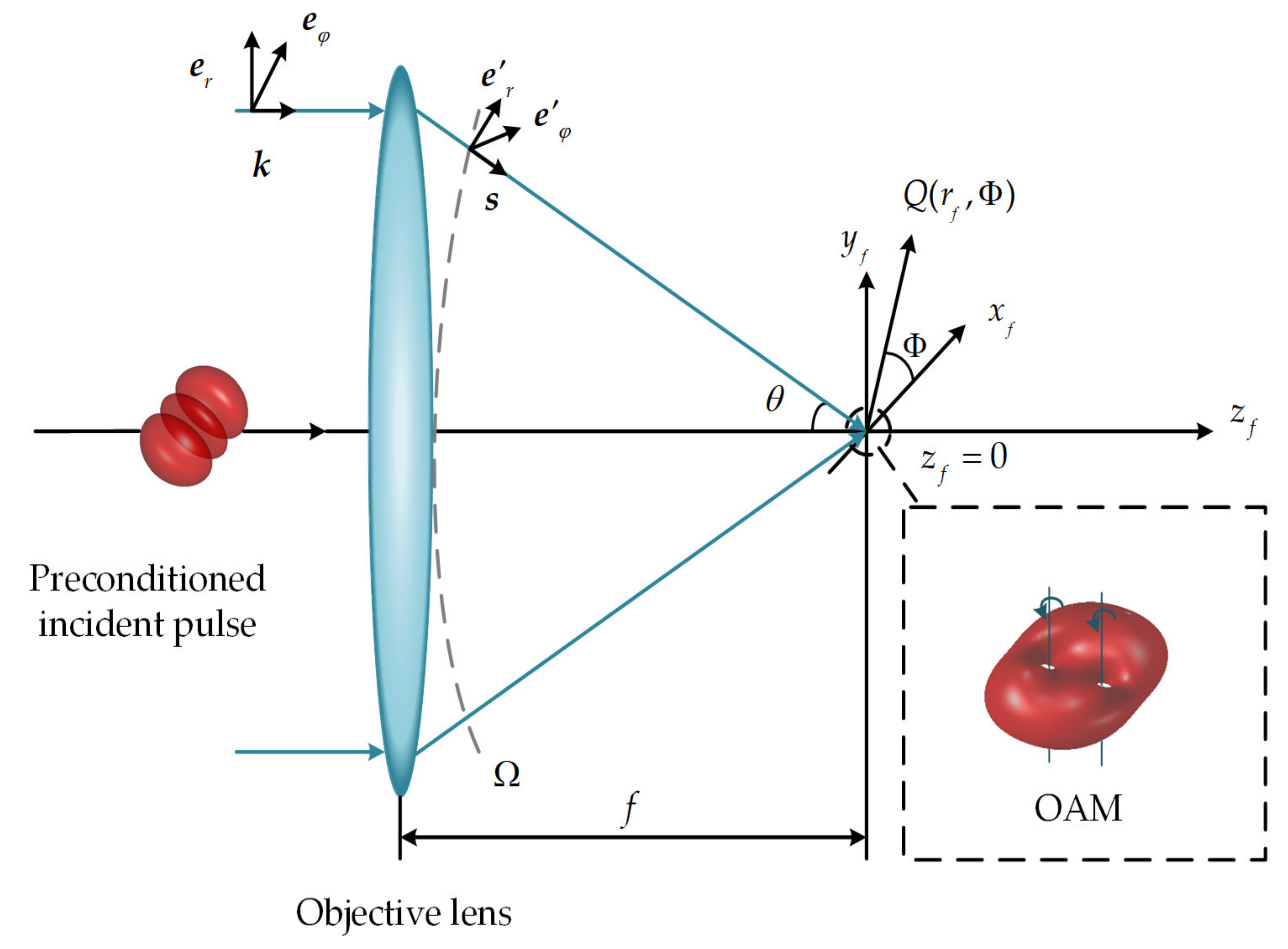
2. Methods
3. Results
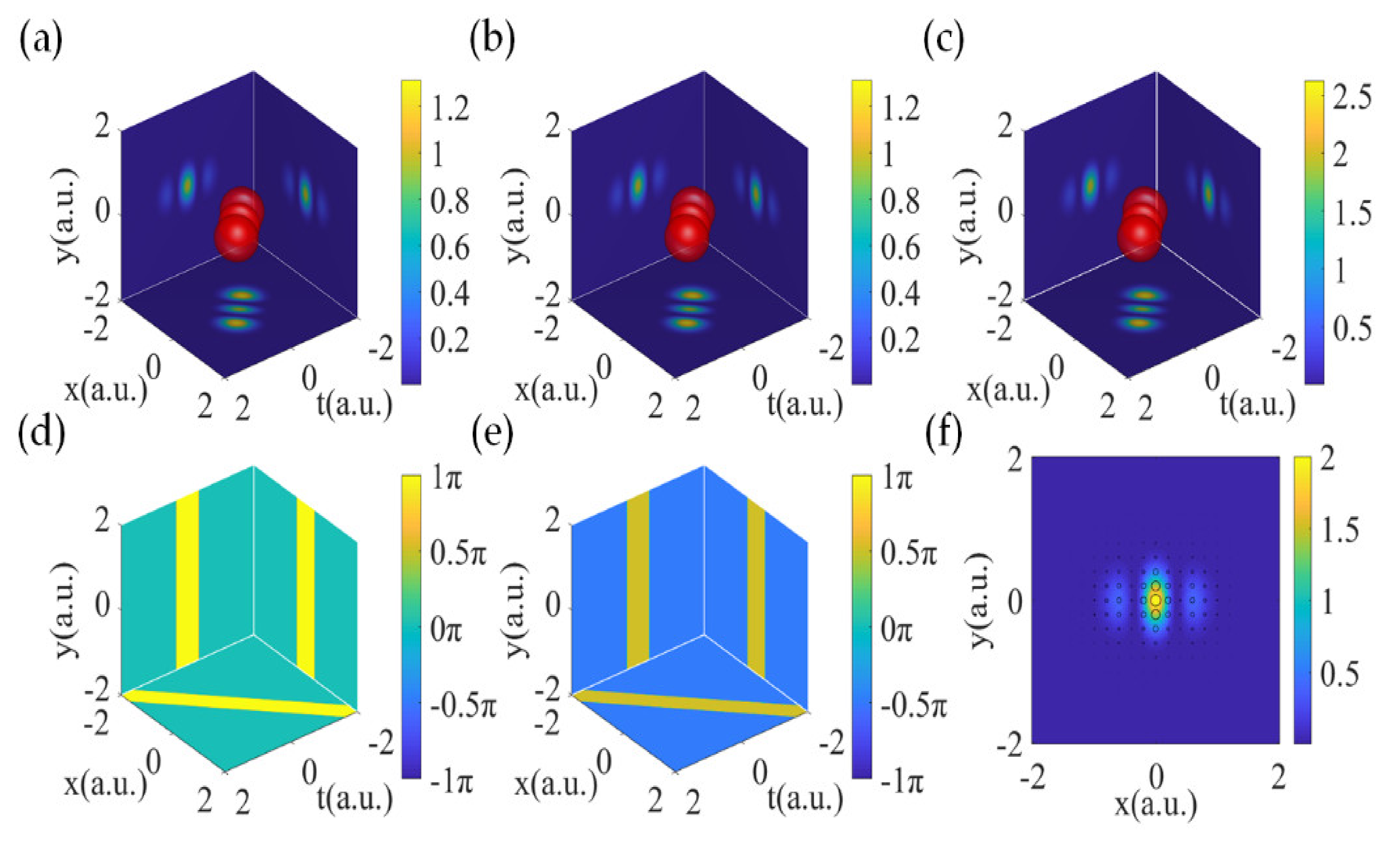
3.1. Transversely Polarized Components
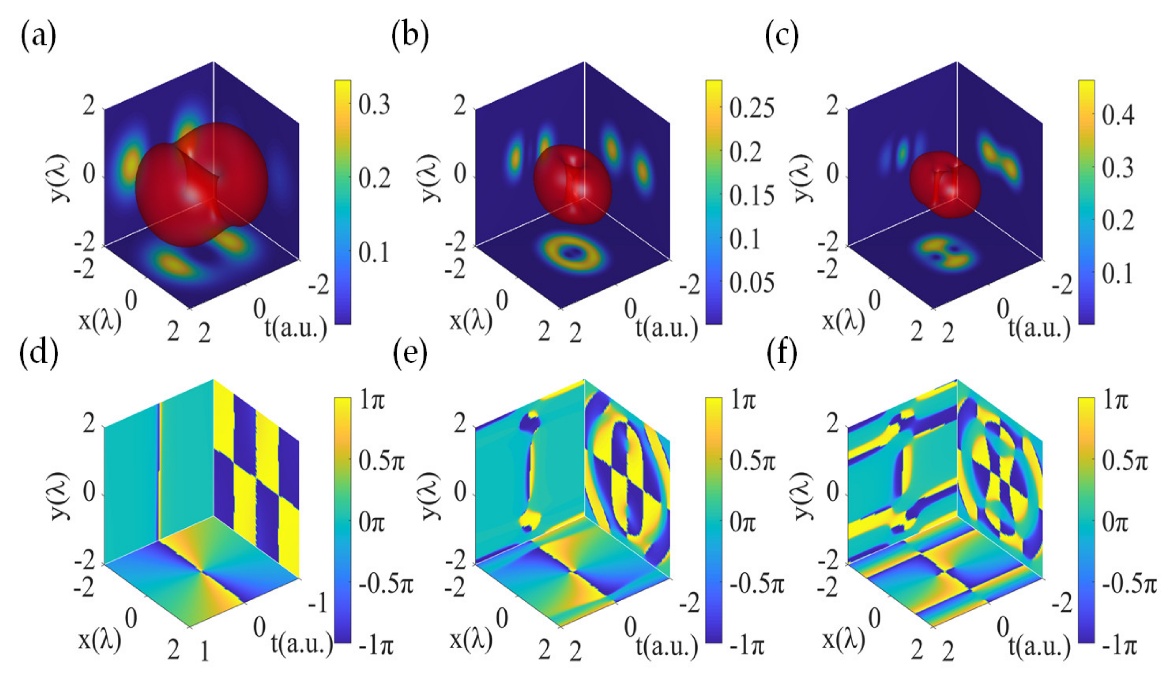
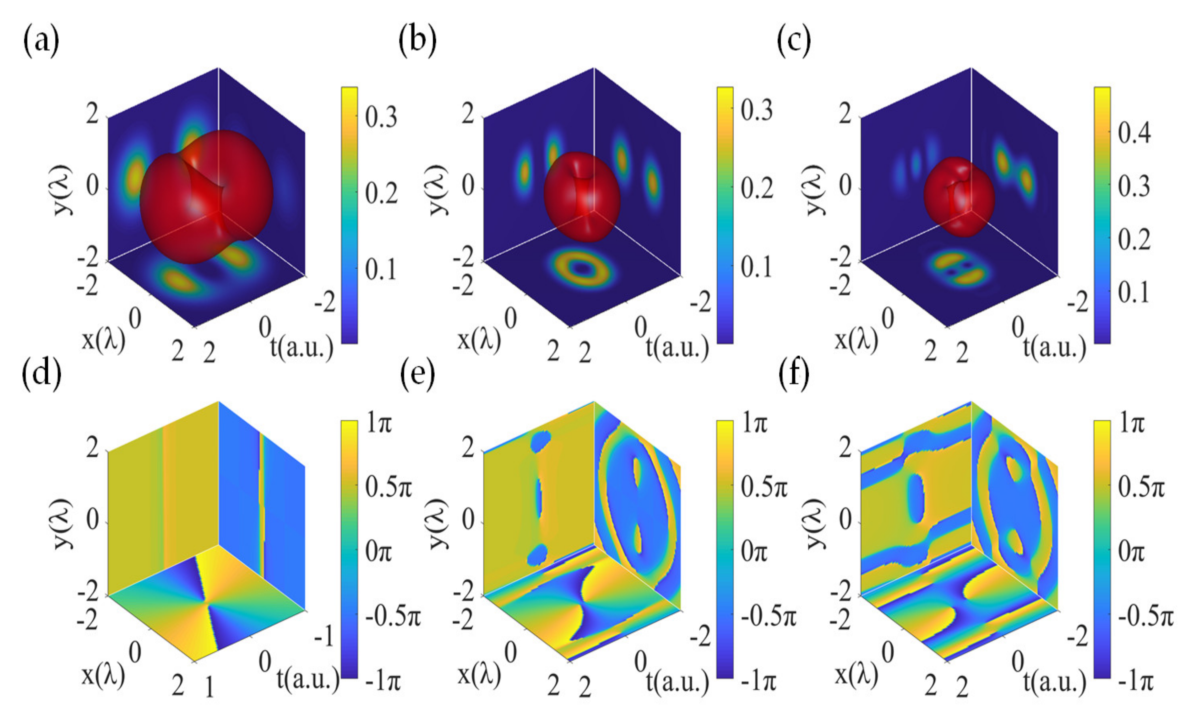
3.2. Longitudinally Polarized Components
4. Discussion
Author Contributions
Funding
Institutional Review Board Statement
Data Availability Statement
Conflicts of Interest
References
- Allen, L.; Beijersbergen, M.W.; Spreeuw, R.J.C.; Woerdman, J.P. Orbital Angular Momentum of Light and the Transformation of Laguerre-Gaussian Laser Modes. Phys. Rev. A 1992, 45, 8185–8189. [Google Scholar] [CrossRef]
- Lei, T.; Zhang, M.; Li, Y.R.; Jia, P.; Liu, G.N.; Xu, X.G.; Li, Z.H.; Min, C.J.; Lin, J.; Yu, C.Y.; et al. Massive Individual Orbital Angular Momentum Channels for Multiplexing Enabled by Dammann Gratings. Light Sci. Appl. 2015, 4, e257. [Google Scholar] [CrossRef]
- Gong, L.; Zhao, Q.; Zhang, H.; Hu, X.Y.; Huang, K.; Yang, J.M.; Li, Y.M. Optical orbital-angular-momentum multiplexed data transmission under high scattering. Light Sci. Appl. 2019, 8, 27. [Google Scholar] [CrossRef] [PubMed]
- Liu, Z.W.; Yan, S.; Liu, H.G.; Chen, X.F. Super High-Resolution Recognition of Optical Vortex Modes Assisted by a Deep-Learning Method. Phys. Rev. Lett. 2019, 123, 183902. [Google Scholar] [CrossRef] [PubMed]
- Li, S.J.; Pan, X.Z.; Ren, Y.; Liu, H.Z.; Jing, J.T. Deterministic Generation of Orbital-Angular-Momentum Multiplexed Tripartite Entanglement. Phys. Rev. Lett. 2020, 124, 083605. [Google Scholar] [CrossRef] [PubMed]
- Liu, S.; Lou, Y.; Jing, J. Orbital Angular Momentum Multiplexed Deterministic All-optical Quantum Teleportation. Nat. Commun. 2020, 11, 3875. [Google Scholar] [CrossRef]
- Tamburini, F.; Anzolin, G.; Umbriaco, G.; Bianchini, A.; Barbieri, C. Overcoming the Rayleigh Criterion Limit with Optical Vortices. Phys. Rev. Lett. 2006, 97, 163903. [Google Scholar] [CrossRef]
- Yan, L.; Gregg, P.; Karimi, E.; Rubano, A.; Marrucci, L.; Boyd, R.; Ramachandran, S. Q-plate Enabled Spectrally Diverse Orbital-Angular Momentum Conversion for Stimulated Emission Depletion Microscopy. Optica 2015, 2, 900–903. [Google Scholar] [CrossRef]
- Hoshina, M.; Yokoshi, N.; Ishihara, H. Nanoscale Rotational Optical Manipulation. Opt. Express 2020, 28, 14980–14994. [Google Scholar] [CrossRef]
- Bobkova, V.; Stegemann, J.; Droop, R.; Otte, E.; Denz, C. Optical Grinder: Sorting of Trapped Particles by Orbital Angular Momentum. Opt. Express 2021, 29, 12967–12975. [Google Scholar] [CrossRef]
- Vallone, G.; D’Ambrosio, V.; Sponselli, A.; Slussarenko, S.; Marrucci, L.; Sciarrino, F.; Villoresi, P. Free-space Quantum Key Distribution by Rotation-invariant Twisted Photons. Phys. Rev. Lett. 2014, 113, 060503. [Google Scholar] [CrossRef] [PubMed]
- Viswanathan, N.K.; Inavalli, V. Generation of Optical Vector Beams Using a Two-mode Fiber. Opt. Lett. 2009, 34, 1189–1191. [Google Scholar] [CrossRef] [PubMed]
- Leach, J.; Yao, E.; Padgett, M.J. Observation of the Vortex Structure of a Non-integer Vortex Beam. New J. Phys. 2004, 6, 71. [Google Scholar] [CrossRef]
- Zhang, H.; Zeng, J.; Lu, X.; Wang, Z.; Zhao, C.; Cai, Y. Review on Fractional Vortex Beam. Nanophotonics 2022, 11, 241–273. [Google Scholar] [CrossRef]
- Zhu, L.; Tang, M.; Li, H.; Tai, Y.; Li, X. Optical Vortex Lattice: An Exploitation of Orbital Angular Momentum. Nanophotonics 2021, 10, 2487–2496. [Google Scholar] [CrossRef]
- García-García, J.; Rickenstorff-Parrao, C.; Ramos-García, R.; Arrizón, V.; Ostrovsky, A.S. Simple Technique for Generating the Perfect Optical Vortex. Opt. Lett. 2014, 39, 5305–5308. [Google Scholar] [CrossRef]
- Hernandez-Garcia, C.; Picon, A.; San Roman, J.; Plaja, L. Attosecond Extreme Ultraviolet Vortices from High-Order Harmonic Generation. Phys. Rev. Lett. 2013, 111, 083602. [Google Scholar] [CrossRef]
- Sukhorukov, A.P.; Yangirova, V.V. Spatio-temporal Vortices: Properties, Generation and Recording. Proc. SPIE 2005, 5949, 594906. [Google Scholar]
- Bliokh, K.Y.; Nori, F. Spatiotemporal Vortex Beams and Angular Momentum. Phys. Rev. A 2012, 86, 033824. [Google Scholar] [CrossRef]
- Jhajj, N.; Larkin, I.; Rosenthal, E.W.; Zahedpour, S.; Wahlstrand, J.K.; Milchberg, H.M. Spatiotemporal Optical Vortices. Phys. Rev. X 2016, 6, 031037. [Google Scholar] [CrossRef]
- Hancock, S.W.; Zahedpour, S.; Goffin, A.; Milchberg, H.M. Free-space Propagation of Spatiotemporal Optical Vortices. Optica 2019, 6, 1547–1553. [Google Scholar] [CrossRef]
- Chong, A.; Wan, C.; Chen, J.; Zhan, Q. Generation of Spatiotemporal Optical Vortices with Controllable Transverse Orbital Angular Momentum. Nat. Photonics 2020, 14, 350–354. [Google Scholar] [CrossRef]
- Bliokh, K.Y. Spatiotemporal Vortex Pulses: Angular Momenta and Spin-orbit Interaction. Phys. Rev. Lett. 2021, 126, 243601. [Google Scholar] [CrossRef] [PubMed]
- Hancock, S.W.; Zahedpour, S.; Milchberg, H.M. Second Harmonic Generation of Spatiotemporal Optical Vortices and Conservation of Orbital Angular Momentum. Optica 2021, 8, 594–597. [Google Scholar] [CrossRef]
- Gui, G.; Brooks, N.J.; Kapteyn, H.C.; Murnane, M.M.; Liao, C. Second-harmonic Generation and the Conservation of Spatiotemporal Orbital Angular Momentum of Light. Nat. Photonics 2021, 15, 608–613. [Google Scholar] [CrossRef]
- Huang, S.L.; Wang, P.; Shen, X.; Liu, J. Properties of the Generation and Propagation of Spatiotemporal Optical Vortices. Opt. Express 2021, 29, 26995–27003. [Google Scholar] [CrossRef]
- Hancock, S.W.; Zahedpour, S.; Milchberg, H.M. Mode Structure and Orbital Angular Momentum of Spatiotemporal Optical Vortex Pulses. Phys. Rev. Lett. 2021, 127, 193901. [Google Scholar] [CrossRef]
- Cao, Q.; Chen, J.; Lu, K.; Wan, C.; Chong, A.; Zhan, Q. Sculpturing Spatiotemporal Wavepackets with Chirped Pulses. Photonics Res. 2021, 9, 2261–2264. [Google Scholar] [CrossRef]
- Chen, J.; Wan, C.; Chong, A.; Zhan, Q. Experimental Demonstration of Cylindrical Vector Spatiotemporal Optical Vortex. Nanophotonics 2021, 10, 4489–4495. [Google Scholar] [CrossRef]
- Chen, J.; Wan, C.; Chong, A.; Zhan, Q. Subwavelength Focusing of a Spatio-temporal Wave Packet with Transverse Orbital Angular Momentum. Opt. Express 2020, 28, 18472–18478. [Google Scholar] [CrossRef]
- Wan, C.; Chen, J.; Chong, A.; Zhan, Q. Generation of Ultrafast Spatiotemporal Wave Packet Embedded with Time-varying Orbital Angular Momentum. Sci. Bull. 2020, 65, 1334–1336. [Google Scholar] [CrossRef] [PubMed]
- Chen, J.; Yu, L.; Wan, C.; Zhan, Q. Spin-Orbit Coupling within Tightly Focused Circularly Polarized Spatiotemporal Vortex Wavepacket. ACS Photonics 2022, 9, 793–799. [Google Scholar] [CrossRef]
- Mazanov, M.; Sugic, D.; Alonso, M.A.; Nori, F.; Bliokh, K.Y. Transverse Shifts and Time Delays of Spatiotemporal Vortex Pulses Reflected and Refracted at a Planar Interface. Nanophotonics 2022, 11, 737–744. [Google Scholar] [CrossRef]
- Wang, H.; Guo, C.; Jin, W.; Song, A.; Fan, S. Engineering Arbitrarily Oriented Spatiotemporal Optical Vortices Using Transmission Nodal Lines. Optica 2021, 8, 966–971. [Google Scholar] [CrossRef]
- Gui, G.; Brooks, N.J.; Wang, B.; Kapteyn, H.C.; Murnane, M.M.; Liao, C. Single-frame characterization of ultrafast pulses with spatiotemporal orbital angular momentum. ACS Photonics 2022, 9, 2802–2808. [Google Scholar] [CrossRef]
- Helseth, L. Focusing of Atoms with Strongly Confined Light Potentials. Opt. Commun. 2002, 212, 343–352. [Google Scholar] [CrossRef]


Disclaimer/Publisher’s Note: The statements, opinions and data contained in all publications are solely those of the individual author(s) and contributor(s) and not of MDPI and/or the editor(s). MDPI and/or the editor(s) disclaim responsibility for any injury to people or property resulting from any ideas, methods, instructions or products referred to in the content. |
© 2023 by the authors. Licensee MDPI, Basel, Switzerland. This article is an open access article distributed under the terms and conditions of the Creative Commons Attribution (CC BY) license (https://creativecommons.org/licenses/by/4.0/).
Share and Cite
Chen, J.; Kuai, S.; Chen, G.; Yu, L.; Zhan, Q. Dynamical Modulation of Transverse Orbital Angular Momentum in Highly Confined Spatiotemporal Optical Vortex. Photonics 2023, 10, 148. https://doi.org/10.3390/photonics10020148
Chen J, Kuai S, Chen G, Yu L, Zhan Q. Dynamical Modulation of Transverse Orbital Angular Momentum in Highly Confined Spatiotemporal Optical Vortex. Photonics. 2023; 10(2):148. https://doi.org/10.3390/photonics10020148
Chicago/Turabian StyleChen, Jian, Siyu Kuai, Guoliang Chen, Lihua Yu, and Qiwen Zhan. 2023. "Dynamical Modulation of Transverse Orbital Angular Momentum in Highly Confined Spatiotemporal Optical Vortex" Photonics 10, no. 2: 148. https://doi.org/10.3390/photonics10020148
APA StyleChen, J., Kuai, S., Chen, G., Yu, L., & Zhan, Q. (2023). Dynamical Modulation of Transverse Orbital Angular Momentum in Highly Confined Spatiotemporal Optical Vortex. Photonics, 10(2), 148. https://doi.org/10.3390/photonics10020148