Lie Symmetry Classification, Optimal System, and Conservation Laws of Damped Klein–Gordon Equation with Power Law Non-Linearity

Abstract

We used the classical Lie symmetry method to study the damped Klein–Gordon equation (Kge) with power law non-linearity $u_{tt}+\alpha \left(u\right)u_t={\left(u^{\beta }{u}_x\right)}_x+f\left(u\right)$. We carried out a complete Lie symmetry classification by finding forms for $\alpha \left(u\right)$ and $f\left(u\right)$. This led to various cases. Corresponding to each case, we obtained one-dimensional optimal systems of subalgebras. Using the subalgebras, we reduced the Kge to ordinary differential equations and determined some invariant solutions. Furthermore, we obtained conservation laws using the partial Lagrangian approach.

1. Introduction

The aim of this study was to perform a complete Lie point symmetry classification of the (1 + 1)-dimensional damped Klein–Gordon equation (Kge) with power law non-linearity:

$$u_{tt}+\alpha \left(u\right)u_t={\left(u^{\beta }{u}_x\right)}_x+f\left(u\right),\beta \ne 0,$$

(1)

where $\alpha \left(u\right)u_t$ and $u^{\beta }$ represent the damping and power law non-linearity terms, respectively. The presence of the terms $\alpha \left(u\right)u_t$, ${\left(u^{\beta }{u}_x\right)}_x$, and $f\left(u\right)$ introduces non-linearity into the equation, making it pertinent to analyze the non-linear dynamics of the significant system. For example, the non-linear term $u^{\beta }{u}_x$ can introduce phenomena like solitons and shock waves. Equation (1) has a wide range of physical applications in quantum mechanics, non-linear dynamics, wave propagation, and applied mathematics research. In general, this equation presents an interplay between non-linearities and wave-like behavior, making it all-inclusive, from quantum field theory, particle physics, quantum mechanics, and mathematical physics to applied mathematics. The second-order partial differential Equation (1) is an extended form of the Klein–Gordon equation:

$$u_{tt}=u_{xx}+f\left(u\right),$$

(2)

which appears in quantum mechanics and describes the motion of spinless scalar particles. Equation (1) can be constituted as a test case in applied mathematical research for analytical as well as numerical methods for solving Pdes. To find the Lie point symmetries of (1), we followed the classical Lie group approach proposed by Sophus Lie in 1881. The group symmetry method is feasible to find exact solutions, conservation laws when a Lagrangian exists, and reductions of differential equations. This approach is efficient to deal with linear and non-linear partial differential equations (Pdes) as well as ordinary differential equations (Odes). The reader is referred to the well-known books of Ovsiannikov [1], Bluman [2,3], Olver [4], and Ibragimov [5] for detailed explanations of this versatile method.

The classical approach has been widely applied to study the group properties of various non-linear partial differential equations, including the wave and heat equations, see for example [1,6]. Azad et al. investigated Equation (2) by the classical Lie approach. They performed group classification and obtained the symmetry generators for each case. Additionally, they provided reductions and some exact solutions of the Klein–Gordon equation [7].

This study involved finding the Lie point symmetries for all viable forms of the arbitrary functions and deducing the optimal system of one-dimensional subalgebras as well as the local conservation laws via the partial Lagrangian approach. Reducing the number of independent variables of Pdes and constructing conservation laws are two important applications for identifying the solutions and physical properties of the governing equations. We found the reductions of (1) via the optimal system of one-dimensional subalgebras, as these provided the possible combinations of Lie symmetries that are helpful for determining the reduced form of the original differential equation. The two main methods for finding the optimal system include the adjoint representation method presented by Olver [4] and the global matrix method given by Ovsiannikov [1]. In general, Lie symmetry analysis is indeed a flexible method to study diverse aspects of differential equations, including the identification of conserved vectors and the deduction of solitary wave solutions. Solitary waves frequently appear in different physical systems, like plasma physics, non-linear dynamics, and water waves. Also, conservation laws are highly important as they are used to find non-local symmetries, detect the integrability of Pdes, and check the accuracy and existence of numerical solution methods. The conserved currents are useful for finding the solutions of non-linear and linear differential equations by double reduction theory. Bokhari et al. proposed the generalization of double reduction theory to obtain an invariant solution for a non-linear system of qth order Pdes [8,9].

A number of approaches are available to find the conservation laws of differential equations. One of these methods is the partial Lagrangian approach introduced by Mahomed and Kara [10], which is an efficient technique to find the conservation laws without the existence of a typical Lagrangian. Other methods include the Noether approach [11], which relies on the existence of a Lagrangian; the multiplier approach; and the direct method [12].

Tian et al. proposed an effective, efficient, and direct approach to investigate symmetry-preserving discretization for a class of generalized higher-order equations and also promulgated the open problem regarding symmetries and multipliers relating to conservation laws [13]. Moreover, Tian et al. studied the conservation laws and solitary wave solutions for a fourth-order non-linear generalized Boussinesq water wave equation in [14] as well as the chiral non-linear Schrodinger equation in $(2+1)$ dimensions, see [15]. The authors also resolved the non-local symmetries and soliton–conoidal interaction solutions of the $(2+1)$-dimensional Boussinesq equation in [16].

This paper is arranged as follows: in Section 2, we find the complete Lie point symmetries of the damped Klein–Gordon Equation (1) by deducing the particular forms of unknown arbitrary functions $\alpha \left(u\right)$ and $f\left(u\right)$. In Section 3, we list the optimal system of one-dimensional subalgebras and corresponding reductions for all the cases that arose in Section 1. The graphs of some of the exact solutions are displayed as well. In Section 4, the conservation laws, via the partial Lagrangian approach, are presented.

2. Lie Symmetry Classification

The principal Lie point symmetries of (1) are obtained in this section. Also, for all possible forms of smooth functions $f\left(u\right)$ and $\alpha \left(u\right)$, a complete Lie group classification is performed. For this, we take the Lie point symmetry generator as

$$\mathcal{X}={\xi }^1(t,x,u)\frac{\partial }{\partial t}+{\xi }^2(t,x,u)\frac{\partial }{\partial x}+\zeta (t,x,u)\frac{\partial }{\partial u}.$$

(3)

According to Lie group theory, the invariance condition leading to Lie point symmetries of (1) is

$${\mathcal{X}}^{\left[2\right]}\left(u_{tt}+\alpha \left(u\right)u_t-{\left(u^{\beta }{u}_x\right)}_x-f\left(u\right)\right){|}_{Equation\left(1\right)=0}=0,$$

(4)

where ${\mathcal{X}}^{\left[2\right]}$ is the second-order prolongation required, which is up to the order of Equation (1) and is given by

$${\mathcal{X}}^{\left[2\right]}=\mathcal{X}+{\phi }^i\frac{\partial }{\partial u_i}+{\phi }^{ij}\frac{\partial }{\partial u_{ij}},$$

(5)

where

$$\begin{array}{cc}\hfill {\phi }^i& ={\mathcal{D}}_i\left(\zeta \right)-u_j{\mathcal{D}}_i{\xi }^j,\hfill \\ \hfill {\phi }^{ij}& ={\mathcal{D}}_j\left({\phi }^i\right)-u_{ji}{\mathcal{D}}_i{\xi }^j,i,j=1,2,\hfill \end{array}$$

and ${\mathcal{D}}_i$ is the total derivative operator

$${\mathcal{D}}_i=\frac{\partial }{\partial x^i}+u_i\frac{\partial }{\partial u}+\dots ,(x^1,x^2)=(t,x).$$

We arrive at the following determining system of Pdes, after expansion of (4) and comparison of the coefficients of independent partial derivatives equated to zero,

$$\begin{array}{cc}\hfill {\zeta }_{uu}=0,{\xi }_x^1=0,{\xi }_t^2& =0,\hfill \end{array}$$

(6)

$$\begin{array}{cc}\hfill -2\beta u^{\beta -1}{\zeta }_x-(2{\zeta }_{xu}-{\xi }_{xx}^2)u^{\beta }& =0,\hfill \end{array}$$

(7)

$$\begin{array}{cc}\hfill \zeta {\alpha }_u+{\xi }_t^1\alpha \left(u\right)+2{\zeta }_{tu}-{\xi }_{tt}^1& =0,\hfill \end{array}$$

(8)

$$\begin{array}{cc}\hfill -\beta (\beta -1)\zeta u^{\beta -2}-\beta u^{\beta -1}{\zeta }_u+2\beta u^{\beta -1}({\xi }_x^2-{\xi }_t^1)& =0,\hfill \end{array}$$

(9)

$$\begin{array}{cc}\hfill -\zeta \beta u^{\beta -1}+2({\xi }_x^2-{\xi }_t^1)u^{\beta }& =0,\hfill \end{array}$$

(10)

$$\begin{array}{cc}\hfill -\zeta f_u+\alpha \left(u\right){\zeta }_t+({\zeta }_u-2{\xi }_t^1)f\left(u\right)+{\zeta }_{tt}-u^{\beta }{\zeta }_{xx}& =0.\hfill \end{array}$$

(11)

By means of Equation (10), we easily have

$$\zeta =\frac{2}{\beta }({\xi }_x^2-{\xi }_t^1)u.$$

(12)

Invoking Equations (7) and (12), we obtain

$$(3\beta +4){\xi }_{xx}^2=0.$$

(13)

The following cases arise from Equation (13)

1.

${\xi }_{xx}^2=0,$ $\beta \ne -\frac{4}{3}$,

2.

$(3\beta +4)=0.$

Case 1: 

 ${\xi }_{xx}^2=0$ and  $\beta \ne -\frac{4}{3}$

This implies

$${\xi }^2=c_{1}x+c_2.$$

Using (12) in (8), we obtain

$$\frac{2}{\beta }(c_1-{\xi }_t^1)u{\alpha }_u+\alpha {\xi }_t^1-(\frac{4}{\beta }+1){\xi }_{tt}^1=0.$$

(14)

If $\alpha \left(u\right)$ is an arbitrary function of u, then

$${\xi }^1=0,$$

which then gives from (14)

$$c_1=0,$$

implying that $\zeta =0.$ Hence, for arbitrary $\alpha \left(u\right)$, Equation (1) has a two-dimensional principal Lie algebra, spanned by

$${\mathcal{X}}_1=\frac{\partial }{\partial x},{\mathcal{X}}_2=\frac{\partial }{\partial t}.(\alpha \ne 0)$$

Now, for the complete classification of (1), we look for all the choices for which the principal Lie algebra extends. For this, differentiation of (14) w.r.t. u gives

$$\frac{2}{\beta }(c_1-{\xi }_t^1)u{\alpha }_{uu}+\left(\frac{2}{\beta }(c_1-{\xi }_t^1)+{\xi }_t^1\right){\alpha }_u=0.$$

(15)

Two subcases arise here.

1.1. 

  ${\alpha }_u\ne 0,$

1.2. 

  ${\alpha }_u=0.$

Subcase 1.1: 

  ${\alpha }_u\ne 0$

In this case, from (15), we have

$$\frac{2}{\beta }(c_1-{\xi }_t^1)u\frac{{\alpha }_{uu}}{{\alpha }_u}+\frac{2}{\beta }(c_1-{\xi }_t^1)+{\xi }_t^1=0.$$

(16)

We now consider

$$u\frac{{\alpha }_{uu}}{{\alpha }_u}=k.$$

This gives

$$\alpha =\frac{k_1}{k+1}{u}^{k+1}+k_2,k_1\ne 0as{\alpha }_u\ne 0.$$

(17)

Here, $k_1$, $k_2$ and k are constants. From this, we have two more subcases, viz.

1.1.1. 

  $k\ne -1,$

1.1.2. 

  $k=-1.$

Subcase 1.1.1: 

  $k\ne -1$

By invoking (17) in (14) and equating the coefficients of different powers of u, we arrive at

$$2c_1(k+1)-2{\xi }_t^1(k+1)+\beta {\xi }_t^1=0,$$

(18)

which gives

$${\xi }^1=-\frac{2(k+1)}{\beta -2(k+1)}{c}_{1}t+c_3,\beta \ne 2(k+1)$$

provided $k_2=0$, otherwise, there are two symmetry generators, ${\mathcal{X}}_1$ and ${\mathcal{X}}_2$, which form the principal algebra. Equation (12) implies

$$\zeta =\frac{2}{\beta -2(k+1)}{c}_{1}u.$$

Now, from (11), we have

$$f\left(u\right)=f_1{u}^{2k+3}.$$

The principal algebra in this case extends to the three-dimensional algebra spanned by ${\mathcal{X}}_1$ and ${\mathcal{X}}_2$ in addition to

$${\mathcal{X}}_3=x\frac{\partial }{\partial x}-\frac{2(k+1)}{\beta -2(k+1)}t\frac{\partial }{\partial t}+\frac{2}{\beta -2(k+1)}u\frac{\partial }{\partial u},$$

provided $\beta \ne 2(k+1).$

Subcase 1.1.1.1: 

  $\beta =2(k+1)$

If $\beta =2(k+1)$, then (18) gives $c_1=0$ as $k\ne -1$. This implies ${\xi }^2=c_2$ and

$$\zeta =-\frac{2}{\beta }{\xi }_t^{1}u.$$

By inserting this value of $\zeta$ into (8), we arrive at

$$(-\frac{2}{\beta }u{\alpha }_{uu}+(1-\frac{2}{\beta }){\alpha }_u){\xi }_t^1=0.$$

In this case, we have

$$-\frac{2}{\beta }u{\alpha }_{uu}+(1-\frac{2}{\beta }){\alpha }_u=0.$$

However, if ${\xi }_t^1=0$, there is only the principal algebra generated by ${\mathcal{X}}_1$ and ${\mathcal{X}}_2.$ After some manipulation, we deduce

$$\alpha =\frac{k_1}{k+1}{u}^{k+1},k\ne -1$$

and from (11), we determine

$$\frac{1}{k+1}[u{f}_u+(\frac{1}{k+1}{k}_1{u}^{k+1}+k_2)(-\frac{{\xi }_{tt}^1}{{\xi }_t^1}u)-\frac{{\xi }_{ttt}^1}{{\xi }_t^1}u-(2k+3)f]=0.$$

(19)

Differentiating w.r.t. t and u, respectively, gives

$$k_1{u}^k{\left(\frac{{\xi }_{tt}^1}{{\xi }_t^1}\right)}_t=0,$$

which in turn implies

$$\frac{{\xi }_{tt}^1}{{\xi }_t^1}=c_{3}as{k}_1\ne 0.$$

The resultant equation yields

$${\xi }^1=-\frac{c_4}{c_3}+c_5{e}^{-c_{3}t},c_3\ne 0.$$

(20)

From (19), we obtain

$$f\left(u\right)=-\frac{1}{{(k+1)}^2}{c}_3{k}_1{u}^{k+1}+f_1{u}^{2k+3}-\frac{1}{2(k+1)}(k_2{c}_3+c_3^2)u.$$

Here, $f_1$ is constant. For these forms of $\alpha \left(u\right)$ and $f\left(u\right)$, the principal algebra occurs, since the determining system gives $c_5=0.$

Subcase 1.1.1.1.1: 

If $\beta =2(k+1)$  and  $c_3=0$

The infinitesimals in this case are

$${\xi }^1=c_{4}t+c_5,\zeta =-\frac{1}{k+1}{c}_{4}u,k\ne -1.$$

The algebra in this case extends the principal algebra as we also have

$${\mathcal{X}}_3=t\frac{\partial }{\partial t}-\frac{1}{(k+1)}u\frac{\partial }{\partial u},$$

where

$$f\left(u\right)=f_1{u}^{2k+3}and\alpha \left(u\right)=\frac{k_1}{k+1}{u}^{k+1}.$$

Subcase 1.1.2: 

$k=-1$

This leads to

$$\alpha \left(u\right)=k_{1}ln\left(u\right)+k_2,$$

where $k_1$ and $k_2$ are constants. Substituting in (14) and equating the coefficients of different powers of u, we obtain the following infinitesimals:

$${\xi }^1=a_1,{\xi }^2=c_{2}and\zeta =0.$$

This results in ${\mathcal{X}}_1$ and ${\mathcal{X}}_2$ only.

Subcase 1.2: 

 ${\alpha }_u=0$

If ${\alpha }_u=0$, then

$$\alpha =k\left(constant\right).$$

For this form of $\alpha \left(u\right)$, (14) results in

$$k{\xi }_t^1-(\frac{4}{\beta }+1){\xi }_{tt}^1=0.$$

(21)

After some manipulations, we find

$${\xi }_t^1-\frac{\beta k}{4+\beta }{\xi }^1=-\frac{\beta }{4+\beta }{a}_1,\beta \ne -4.$$

From here, we arrive at the following two subcases.

Subcase 1.2.1: 

 $\beta \ne -4$

In this subcase, we have

$${\xi }^1=\frac{1}{k}{a}_1+a_2{e}^{\frac{\beta k}{4+\beta }t},k\ne 0.$$

Now, (11) gives

$$c_1(-u{f}_u+f)=0$$

which further leads to two subcases.

Case A: 

 $c_1=0$

This yields the following form of f

$$f\left(u\right)=-\frac{4+2\beta }{{(4+\beta )}^2}{k}^{2}u+f_1{u}^{1+\beta }.$$

The algebra in this case is three-dimensional, generated by

$${\mathcal{X}}_1=\frac{\partial }{\partial x},{\mathcal{X}}_2=\frac{1}{k}\frac{\partial }{\partial t},$$

$${\mathcal{X}}_3=e^{\frac{\beta k}{4+\beta }t}\left(\frac{\partial }{\partial t}-\frac{2k}{4+\beta }u\frac{\partial }{\partial u}\right).$$

Case B: 

 $c_1\ne 0$

In this case, we deduce

$$f\left(u\right)=-\frac{4+2\beta }{{(4+\beta )}^2}{k}^{2}u,$$

where the infinitesimals

$${\xi }^2=c_{1}x+c_2,{\xi }^1=\frac{1}{k}{a}_1+a_2{e}^{\frac{\beta k}{4+\beta }t},$$

$$\zeta =\frac{2}{\beta }(c_1-\frac{\beta k}{4+\beta }{e}^{\frac{\beta k}{4+\beta }t}{a}_2)u,$$

generate a four-dimensional Lie algebra with generator

$${\mathcal{X}}_4=x\frac{\partial }{\partial x}+\frac{2}{\beta }u\frac{\partial }{\partial u},$$

together with ${\mathcal{X}}_1$, ${\mathcal{X}}_2$ and ${\mathcal{X}}_3$ from Case A.

Subcase 1.2.1.1: 

 $\beta \ne -4,$ $k=0$

If $k=0$ then $\alpha =0.$ Therefore, (21) yields

$${\xi }^1=c_{3}t+c_4.$$

Now from (11), we obtain

$$f\left(u\right)=f_1{u}^{1-\beta k_1},$$

and this gives a three-dimensional Lie algebra spanned by the principal algebra in addition to

$${\mathcal{X}}_3=x\frac{\partial }{\partial x}+\frac{k_1}{(k_1+1)}t\frac{\partial }{\partial t}+\frac{2}{\beta (k_1+1)}u\frac{\partial }{\partial u}.$$

Herein, $f_1$ and $k_1$ are constants.

Subcase 1.2.2: 

 $\beta =-4$

For this case,

$${\xi }^1=\frac{1}{k}{a}_1,k\ne 0$$

leads to two different subcases.

Subcase 1.2.2.1: 

 $\beta =-4,$  $k\ne 0$

Here, we have

$$f\left(u\right)=f_{1}u.$$

For these forms of the functions, the principal algebra extends to three-dimensional with

$${\mathcal{X}}_3=x\frac{\partial }{\partial x}-\frac{1}{2}u\frac{\partial }{\partial u},$$

along with ${\mathcal{X}}_1$, ${\mathcal{X}}_2$ from Case A.

Subcase 1.2.2.2: 

 $\beta =-4,$  $k=0$

In this case, ${\xi }^1$ is undetermined. Differentiating (11) twice with respect to u, we find

$$(c_1-5{\xi }_t^1)g+(c_1-{\xi }_t^1)u{g}_u=0$$

(22)

and by differentiation of the resulting equation w.r.t. t, we have

$${\xi }_{tt}^1(5g+u{g}_u)=0,$$

where $g=f_{uu}.$

This gives rise to two subcases.

Case C: 

 ${\xi }_{tt}^1=0$

One has

$${\xi }^1=c_{3}t+c_4,$$

and

$$f\left(u\right)=f_2{u}^{f_1}.$$

The algebra in this case is spanned by ${\mathcal{X}}_1$, ${\mathcal{X}}_2$ and

$${\mathcal{X}}_3=x\frac{\partial }{\partial x}+\frac{f_1-1}{(f_1+3)}t\frac{\partial }{\partial t}-\frac{2}{(f_1+3)}u\frac{\partial }{\partial u}.$$

Here, $f_1$ and $f_2$ are constants.

Case D: 

 $5g+u{g}_u=0$

In this case, we have

$$g\left(u\right)=ln\left(g_1{u}^{-5}\right),$$

and from (22), we obtain

$${\xi }_t^1=0=c_1,$$

which results in ${\mathcal{X}}_1$ and ${\mathcal{X}}_2$.

Case 2: 

 $\beta =-\frac{4}{3}$  and  ${\xi }_{xx}^2\ne 0$

For this case, (12) becomes

$$\zeta =-\frac{3}{2}({\xi }_x^2-{\xi }_t^1)u.$$

(23)

Now from (8), we have

$$-\frac{3}{2}({\xi }_x^2-{\xi }_t^1)u{\alpha }_u+\alpha {\xi }_t^1+2{\xi }_{tt}^1=0$$

(24)

and differentiation w.r.t. u yields

$$(5{\xi }_t^1-3{\xi }_x^2){\alpha }_u+3({\xi }_t^1-{\xi }_x^2)u{\alpha }_{uu}=0.$$

(25)

We then need to consider the following subcases:

2.1. 

 ${\alpha }_u=0.$

2.2. 

 ${\alpha }_u\ne 0,$

Subcase 2.1: 

 ${\alpha }_u=0$

This implies

$$\alpha \left(u\right)=A\left(constant\right).$$

which reduces (24) to

$${\xi }_t^{1}A+2{\xi }_{tt}^1=0,$$

(26)

and admits the solution

$${\xi }^1=\frac{2}{A}{c}_1+c_2{e}^{-\frac{A}{2}t},A\ne 0.$$

Subcase 2.1.1: 

 $A=0$

From (26),

$${\xi }^1=c_{1}t+c_2.$$

Now from Equations (11) and (23), we obtain

$$3({\xi }_x^2-c_1)u{f}_u+3u^{-1/3}{\xi }_{xxx}^2-(3{\xi }_x^2+c_1)f=0$$

(27)

and differentiating this w.r.t. u, we arrive at

$$-2c_1{f}_u-u^{-4/3}{\xi }_{xxx}^2+(3{\xi }_x^2-c_1)u{f}_{uu}=0.$$

(28)

For arbitrary $f\left(u\right)$, only the principal algebra occurs. For $f\left(u\right)$ not arbitrary, differentiating (28) with respect to x, we find

$$3{\xi }_{xx}^2{u}^{7/3}{f}_{uu}-{\xi }_{xxxx}^2=0.$$

(29)

We consider

$$F_1=u^{7/3}{f}_{uu},$$

which gives

$$f\left(u\right)=\frac{9}{4}{F}_1{u}^{-1/3}+F_{2}u+F_3,$$

and thus (29) becomes

$$3{\xi }_{xx}^2{F}_1-{\xi }_{xxxx}^2=0.$$

(30)

Here, $F_1$, $F_2$ and $F_3$ are constants. By substituting the values in (27) and comparing the coefficients for different powers of u, we determine the following equations:

$${\xi }_{xxx}^2-3F_1{\xi }_x^2=0,$$

(31)

$$c_1{F}_2=0,$$

(32)

$$(3{\xi }_x^2+c_1)F_3=0.$$

(33)

From (32), we have two possibilities, $c_1=0,$ or $F_2=0.$

Subcase 2.1.1.1: 

 $F_2\ne 0$  and  $c_1=0$

If $c_1=0,$ then from (33), we have

$${\xi }_x^2{F}_2=0.$$

1.

If ${\xi }_x^2=0$ and $F_3\ne 0$, then $\zeta =0$ generates the principal algebra only.

2.

If ${\xi }_x^2\ne 0$ and $F_3=0$, then from Equations (30) and (31), we deduce

$${\xi }^2=-\frac{1}{3F_1}{a}_1+a_2{e}^{\sqrt{3F_1}x}+a_3{e}^{-\sqrt{3F_1}x}.$$

The principal algebra extends to four dimensions generated by

$${\mathcal{X}}_1=-\frac{1}{3F_1}\frac{\partial }{\partial x},{\mathcal{X}}_2=\frac{\partial }{\partial t},$$

$${\mathcal{X}}_3=e^{\sqrt{3F_1}x}(\frac{\partial }{\partial x}-\frac{3\sqrt{3F_1}}{2}u\frac{\partial }{\partial u}),$$

$${\mathcal{X}}_4=e^{-\sqrt{3F_1}x}(\frac{\partial }{\partial x}+\frac{3\sqrt{3F_1}}{2}u\frac{\partial }{\partial u}).$$

Subcase 2.1.1.2:  $F_2=0$ and $c_1\ne 0$

From Equation (33), we have two choices

1.

If ${\xi }_x^2\ne -\frac{1}{3}{c}_1$ and $F_3=0$, the Lie algebra in this case is five-dimensional with

$${\mathcal{X}}_5=t\frac{\partial }{\partial t}+\frac{3}{2}u\frac{\partial }{\partial u},$$

in addition to admitting ${\mathcal{X}}_1$, ${\mathcal{X}}_2$, ${\mathcal{X}}_3$ and ${\mathcal{X}}_4$ from subcase 2.1.1.1, where $f\left(u\right)=\frac{9}{4}{F}_1{u}^{-1/3}.$

2.

If ${\xi }_x^2=-\frac{1}{3}{c}_1$ and $F_3\ne 0$, then the Lie algebra in this case is determined by ${\xi }^2=-\frac{1}{3}{c}_{1}x+a_1$ and $\zeta =2c_{1}u$, which gives

$${\mathcal{X}}_3=t\frac{\partial }{\partial t}-\frac{1}{3}x\frac{\partial }{\partial x}+2u\frac{\partial }{\partial u},$$

along with the principal algebra generators ${\mathcal{X}}_1$ and ${\mathcal{X}}_2$.

Subcase 2.1.2: 

 $A\ne 0$

In this case, again from (27), we find (30), (31) and

$$c_2(F_2+\frac{3}{8}{A}^2)=0,$$

(34)

$$(-6{\xi }_x^2+A{c}_2{e}^{-\frac{A}{2}t})F_3=0.$$

(35)

Herein, different subcases result.

Subcase 2.1.2.1: 

 $c_2=0$  and  $F_2\ne -\frac{3}{8}{A}^2$

If $c_2=0,$ from (35), we have two choices

1. 

If ${\xi }_x^2=0$ and $F_3\ne 0$, we obtain the principal algebra only.

2. 

If ${\xi }_x^2\ne 0$ and $F_3=0$, then the symmetry generators are

$${\mathcal{X}}_2=\frac{2}{A}\frac{\partial }{\partial t},$$

and ${\mathcal{X}}_1$, ${\mathcal{X}}_3$ as well as ${\mathcal{X}}_4$ from subcase 2.1.1.1 (2).

Subcase 2.1.2.2: 

 $F_2=-\frac{3}{8}{A}^2$ and $c_2\ne 0$

In this case, we have two possibilities from (35).

1.

If $F_3=0$, then

$$f\left(u\right)=\frac{9}{4}{u}^{-1/3}{F}_1-\frac{3}{8}{A}^{2}u.$$

For this case, the principal algebra extends to five dimensions, in addition to ${\mathcal{X}}_3$, ${\mathcal{X}}_4$ from subcase 2.1.1.1 (2) one has

$${\mathcal{X}}_5=e^{-\frac{A}{2}t}\left(\frac{\partial }{\partial t}-\frac{3}{4}Au\frac{\partial }{\partial u}\right).$$

2.

If $F_3\ne 0$, then the symmetry generators are ${\mathcal{X}}_1$ and ${\mathcal{X}}_2$ only.

Subcase 2.2: 

 ${\alpha }_u\ne 0$

In this case, from (25), we have

$$\alpha \left(u\right)=\frac{k_1}{k+1}{u}^{k+1}+k_2.$$

Here we have two cases.

Subcase 2.2.1: 

 $k\ne -1$

If $k\ne -1$, then from (24), we deduce

$$3(k+1){\xi }^2-(3k+5){\xi }_t^1=0.$$

(36)

After some manipulations, we have

$$f\left(u\right)=F_2{u}^{2k+3},$$

and obtain the principal algebra along with

$${\mathcal{X}}_3=x\frac{\partial }{\partial x}+\frac{3(k+1)}{3k+5}t\frac{\partial }{\partial t}-\frac{3}{3k+5}u\frac{\partial }{\partial u},$$

provided $k\ne -\frac{5}{3}.$

Subcase 2.2.1.1: 

$k=-5/3$

From (23) and (36), we find

$$k_2{\xi }_t^1+2{\xi }_{tt}^1=0,$$

(37)

with solution

$${\xi }^1=\frac{2}{k_2}{a}_2+a_3{e}^{-\frac{1}{2}{k}_{2}t},$$

provided $k_2\ne 0.$ Thus, from (11), we have

$$f\left(u\right)=\frac{9}{8}{k}_1{k}_2{u}^{1/3}-\frac{3}{16}{k}_2^{2}u+f_1{u}^{-1/3}$$

and

$$\alpha \left(u\right)=-\frac{3}{2}{k}_1{u}^{-2/3}+k_2.$$

These forms of functions result in

$${\mathcal{X}}_1=\frac{\partial }{\partial x},{\mathcal{X}}_2=\frac{2}{k_2}\frac{\partial }{\partial t},$$

$${\mathcal{X}}_3=e^{-\frac{1}{2}{k}_{2}t}\left(\frac{\partial }{\partial t}-\frac{3}{4}{k}_{2}u\frac{\partial }{\partial u}\right).$$

Subsubcase 2.2.1.1.1:   $k_2=0$

In this case, Equation (37) gives

$${\xi }^1=a_{2}t+a_3.$$

And after some calculations, we arrive at

$$f\left(u\right)=f_1{u}^{-1/3}.$$

The algebra in this case is spanned by the principal algebra and

$${\mathcal{X}}_3=t\frac{\partial }{\partial t}+\frac{3}{2}u\frac{\partial }{\partial u}.$$

Subcase 2.2.2:   $k=-1$

This yields

$$\alpha \left(u\right)=k_{1}ln\left(u\right)+k_2,$$

and hence from (14) we derive

$${\xi }^1=a_1,{\xi }^2=c_{2}and\zeta =0.$$

This results in the principal algebra only.

Case 3: 

 $\beta =-\frac{4}{3}$  and  ${\xi }_{xx}^2=0$

This case reduces (25) to

$$(5{\xi }_t^1-3c_1){\alpha }_u+3({\xi }_t^1-c_1)u{\alpha }_{uu}=0$$

Again we consider two subcases.

Subcase 3.1: 

 ${\alpha }_u=0$

This implies

$$\alpha \left(u\right)=k\left(constant\right),$$

which reduces (24) to

$$k{\xi }_t^1+2{\xi }_{tt}^1,$$

leading to two more subcases.

Subcase 3.1.1: 

 $k=0$

Following the usual steps, as we performed in the above cases, we obtain the following form of function f

$$f\left(u\right)=f_1{u}^{\sigma /3},$$

which results in the principal algebra, and additionally

$${\mathcal{X}}_3=x\frac{\partial }{\partial x}+\frac{\sigma -3}{\sigma +1}t\frac{\partial }{\partial t}-\frac{6}{\sigma +1}u\frac{\partial }{\partial u},$$

provided $\sigma \ne -1$ and $\sigma \ne 3.$ Here, $\sigma$ is constant.

1. 

If $\sigma =-1$, then

$$f\left(u\right)=u^{-1/3},$$

which yields the principal algebra and ${\mathcal{X}}_5$ from subcase 2.1.1.2 (1).

2. 

If $\sigma =3$, then

$$f\left(u\right)=f_{1}u$$

and for this form of function we find

$${\mathcal{X}}_3=x\frac{\partial }{\partial x}-\frac{3}{2}u\frac{\partial }{\partial u},$$

in addition to ${\mathcal{X}}_1$ and ${\mathcal{X}}_2$.

Subcase 3.1.2: 

 $k\ne 0$

After some manipulations, we obtain

$$f\left(u\right)=-\frac{3}{4}\frac{\sigma -1}{(3\sigma -7)}(2-\sigma )k^{2}u+f_1{u}^{\sigma },$$

with the Lie algebra in this case being two-dimensional spanned by ${\mathcal{X}}_1$ and ${\mathcal{X}}_2$.

Subcase 3.2: 

 ${\alpha }_u\ne 0$

This case has the same Lie algebra as in Subcases 2.2.1 and 2.2.1.1.

The above classification is summarized in Table 1, Table 2 and Table 3.

Table 1. Complete classification.

Cases	Forms of $\mathit{\alpha }\left(\mathit{u}\right)$	Forms of $\mathit{f}\left(\mathit{u}\right)$	Lie Symmetry Algebra
Case 1
${\xi }_{xx}^2=0,$  $\beta \ne -\frac{4}{3}$	Arbitrary	Arbitrary	${\mathcal{X}}_1=\frac{\partial }{\partial x}$,  ${\mathcal{X}}_2=\frac{\partial }{\partial t}$.
Subcase 1.1:   ${\alpha }_u\ne 0$
	$\alpha =\frac{k_1}{k+1}{u}^{k+1}+k_2,$
	$k_1\ne 0$
1.1.1:  $k\ne -1$
$\beta \ne 2(k+1)$	$\alpha =\frac{k_1}{k+1}{u}^{k+1}$	$f\left(u\right)=f_1{u}^{2k+3}$	${\mathcal{X}}_1,{\mathcal{X}}_2$,   and
			${\mathcal{X}}_3=x\frac{\partial }{\partial x}-\frac{2(k+1)}{\beta -2(k+1)}$ $t\frac{\partial }{\partial t}+\frac{2}{\beta -2(k+1)}u\frac{\partial }{\partial u}$
$c_3\ne 0,$ $\beta =2(k+1)$	$\alpha =\frac{k_1}{k+1}{u}^{k+1}$	$f\left(u\right)=-\frac{1}{{(k+1)}^2}{c}_3{k}_1{u}^{k+1}$ $-\frac{1}{2(k+1)}(k_2+c_3^2)u+f_1{u}^{2k+3}$	${\mathcal{X}}_1,{\mathcal{X}}_2\mathrm{only}.$
$c_3=0,$ $\beta =2(k+1)$	$\alpha =\frac{k_1}{k+1}{u}^{k+1}$	$f\left(u\right)=f_1{u}^{2k+3}$	${\mathcal{X}}_1,{\mathcal{X}}_2$, ${\mathcal{X}}_3=t\frac{\partial }{\partial t}-\frac{1}{(k+1)}u\frac{\partial }{\partial u}$
1.1.2:   $k=-1$
$k=-1$	$\alpha =k_{1}ln\left(u\right)+k_2$		${\mathcal{X}}_1,{\mathcal{X}}_2\mathrm{only}.$
Subcase 1.2:   ${\alpha }_u=0$
	$\alpha =k$
1.2.1:  $\beta \ne -4,k\ne 0$
$\beta \ne -4$,   $c_1=0$	$\alpha =k$	$f\left(u\right)=-\frac{4+2\beta }{{(4+\beta )}^2}{k}^{2}u+f_1{u}^{1+\beta }$	${\mathcal{X}}_1=\frac{\partial }{\partial x},{\mathcal{X}}_2=\frac{1}{k}\frac{\partial }{\partial t}$,
			${\mathcal{X}}_3=e^{\frac{\beta k}{4+\beta }t}\left(\frac{\partial }{\partial t}-\frac{2k}{4+\beta }u\frac{\partial }{\partial u}\right)$
$\beta \ne -4$,   $c_1\ne 0$	$\alpha =k$	$f\left(u\right)=-\frac{4+2\beta }{{(4+\beta )}^2}{k}^{2}u$	${\mathcal{X}}_1=\frac{\partial }{\partial x},{\mathcal{X}}_2=\frac{1}{k}\frac{\partial }{\partial t},$ ${\mathcal{X}}_3=e^{\frac{\beta k}{4+\beta }t}\left(\frac{\partial }{\partial t}-\frac{2k}{4+\beta }u\frac{\partial }{\partial u}\right)$, ${\mathcal{X}}_4=x\frac{\partial }{\partial x}+\frac{2}{\beta }u\frac{\partial }{\partial u}$
1.2.1.1:   $\beta \ne -4,k=0$
	$\alpha =0$	$f\left(u\right)=f_1{u}^{1-\beta k_1}$	${\mathcal{X}}_1,{\mathcal{X}}_2,{\mathcal{X}}_3=x\frac{\partial }{\partial x}+\frac{k_1}{(k_1+1)}t\frac{\partial }{\partial t}+\frac{2}{\beta (k_1+1)}u\frac{\partial }{\partial u}$
1.2.2:   $\beta =-4$
1.2.2.1:   $\beta =-4$,   $k\ne 0$
	$\alpha =k$	$f\left(u\right)=f_{1}u$	${\mathcal{X}}_1=\frac{\partial }{\partial x},{\mathcal{X}}_2=\frac{1}{k}\frac{\partial }{\partial t},$ ${\mathcal{X}}_3=x\frac{\partial }{\partial x}-\frac{1}{2}u\frac{\partial }{\partial u}$
1.2.2.2:   $\beta =-4,k=0$
	$\alpha =0$	$f\left(u\right)=f_2{u}^{f_1}$	${\mathcal{X}}_1,{\mathcal{X}}_2,{\mathcal{X}}_3=x\frac{\partial }{\partial x}+\frac{f_1-1}{(f_1+3)}$ $t\frac{\partial }{\partial t}-\frac{2}{(f_1+3)}u\frac{\partial }{\partial u}$

Table 2. Complete classification.

Cases	Forms of $\mathit{\alpha }\left(\mathit{u}\right)$	Forms of $\mathit{f}\left(\mathit{u}\right)$	Lie Symmetry Algebra
Case 2
${\xi }_{xx}^2\ne 0$,   $\beta =-\frac{4}{3}$	Arbitrary	Arbitrary	${\mathcal{X}}_1=\frac{\partial }{\partial x}$,  ${\mathcal{X}}_2=\frac{\partial }{\partial t}$.
Subcase 2.1:   ${\alpha }_u=0$
	$\alpha =A\left(constant\right)$
2.1.1:   $A=0$
	$\alpha =0$	$f\left(u\right)=\frac{9}{4}{F}_1{u}^{-1/3}+F_{2}u+F_3$
2.1.1.1:   $F_2\ne 0,c_1=0$
$\left(\mathbf{1}\right)c_1=0$,   $F_3\ne 0$	$\alpha =0$	$f\left(u\right)=\frac{9}{4}{F}_1{u}^{-1/3}+F_{2}u+F_3$	${\mathcal{X}}_1=-\frac{1}{3F_1}\frac{\partial }{\partial x},{\mathcal{X}}_2=\frac{\partial }{\partial t}$
$\left(\mathbf{2}\right)c_1=0$,   $F_3=0$	$\alpha =0$	$f\left(u\right)=\frac{9}{4}{F}_1{u}^{-1/3}+F_{2}u$	${\mathcal{X}}_1=-\frac{1}{3F_1}\frac{\partial }{\partial x},{\mathcal{X}}_2=\frac{\partial }{\partial t}$, ${\mathcal{X}}_3=e^{\sqrt{3F_1}x}(\frac{\partial }{\partial x}-\frac{3\sqrt{3F_1}}{2}u\frac{\partial }{\partial u}),$ ${\mathcal{X}}_4=e^{-\sqrt{3F_1}x}(\frac{\partial }{\partial x}+\frac{3\sqrt{3F_1}}{2}u\frac{\partial }{\partial u})$
2.1.1.2:   $F_2=0,c_1\ne 0$
$F_3=0$	$\alpha =0$	$f\left(u\right)=\frac{9}{4}{F}_1{u}^{-1/3}$	${\mathcal{X}}_1,{\mathcal{X}}_2,$ ${\mathcal{X}}_3,{\mathcal{X}}_4\mathrm{from}\mathbf{subcase}$2.1.1.1 (2) in addition to ${\mathcal{X}}_5=t\frac{\partial }{\partial t}+\frac{3}{2}u\frac{\partial }{\partial u}$
$F_3\ne 0$	$\alpha =0$	$f\left(u\right)=\frac{9}{4}{F}_1{u}^{-1/3}+F_3$	${\mathcal{X}}_1,{\mathcal{X}}_2,$  and ${\mathcal{X}}_3=t\frac{\partial }{\partial t}-\frac{1}{3}x\frac{\partial }{\partial x}+2u\frac{\partial }{\partial u}$
2.1.2:   $A\ne 0$
	$\alpha =A$	$f\left(u\right)=\frac{9}{4}{F}_1{u}^{-1/3}+F_{2}u+F_3$
2.1.2.1:   $F_2\ne -\frac{3}{8}{A}^2,c_2=0$
$F_3=0$	$\alpha =A$	$f\left(u\right)=\frac{9}{4}{F}_1{u}^{-1/3}+F_{2}u$	${\mathcal{X}}_2=\frac{2}{A}\frac{\partial }{\partial t},$ ${\mathcal{X}}_1,$ ${\mathcal{X}}_3\mathrm{and}{\mathcal{X}}_4$ from subcase 2.1.1.1 (2)
$F_3\ne 0$	$\alpha =A$	$f\left(u\right)=\frac{9}{4}{F}_1{u}^{-1/3}+F_{2}u+F_3$	${\mathcal{X}}_1,{\mathcal{X}}_2\mathrm{only}.$
2.1.2.2:   $F_2=-\frac{3}{8}{A}^2,c_2\ne 0$
$F_3=0$	$\alpha =A$	$f\left(u\right)=\frac{9}{4}{u}^{-1/3}{F}_1-\frac{3}{8}{A}^{2}u$	${\mathcal{X}}_1,{\mathcal{X}}_2,$ ${\mathcal{X}}_3,{\mathcal{X}}_4\mathrm{from}\mathbf{subcase}$2.1.1.1 (2) in addition to ${\mathcal{X}}_5=e^{-\frac{A}{2}t}\left(\frac{\partial }{\partial t}-\frac{3}{4}Au\frac{\partial }{\partial u}\right)$
$F_3\ne 0$	$\alpha =A$	$f\left(u\right)=\frac{9}{4}{u}^{-1/3}{F}_1-\frac{3}{8}{A}^{2}u+F_3$	${\mathcal{X}}_1,{\mathcal{X}}_2\mathrm{only}.$
Subcase 2.2:   ${\alpha }_u\ne 0$
$\mathbf{2}.\mathbf{2}.\mathbf{1}:$ $k\ne -1$
$k\ne -1,k\ne -\frac{5}{3}$	$\alpha =\frac{k_1}{k+1}{u}^{k+1}+k_2$	$f\left(u\right)=F_2{u}^{2k+3}$	${\mathcal{X}}_1,{\mathcal{X}}_2,$  ${\mathcal{X}}_3=x\frac{\partial }{\partial x}+\frac{3(k+1)}{3k+5}$ $t\frac{\partial }{\partial t}-\frac{3}{3k+5}u\frac{\partial }{\partial u}$
$k\ne -1,k=-\frac{5}{3},k_2\ne 0$	$\alpha =-\frac{3}{2}{k}_1{u}^{-2/3}+k_2$	$f\left(u\right)=\frac{9}{8}{k}_1{k}_2{u}^{1/3}-\frac{3}{16}{k}_2^{2}u+$ f1u−1/3	${\mathcal{X}}_1=\frac{\partial }{\partial x},{\mathcal{X}}_2=\frac{2}{k_2}\frac{\partial }{\partial t},$  ${\mathcal{X}}_3=e^{-\frac{1}{2}{k}_{2}t}\left(\frac{\partial }{\partial t}-\frac{3}{4}{k}_{2}u\frac{\partial }{\partial u}\right)$
$k\ne -1,k=-\frac{5}{3},k_2=0$	$\alpha =-\frac{3}{2}{k}_1{u}^{-2/3}$	$f\left(u\right)=f_1{u}^{-1/3}$	${\mathcal{X}}_1,{\mathcal{X}}_2,{\mathcal{X}}_3=t\frac{\partial }{\partial t}+\frac{3}{2}u\frac{\partial }{\partial u}$
$\mathbf{2}.\mathbf{2}.\mathbf{2}:$ $k=-1$
$k=-1$	$\alpha \left(u\right)=k_{1}ln\left(u\right)+k_2$		${\mathcal{X}}_1,{\mathcal{X}}_2\mathrm{only}.$

Table 3. Complete classification.

Cases	Forms of $\mathit{\alpha }\left(\mathit{u}\right)$	Forms of $\mathit{f}\left(\mathit{u}\right)$	Lie Symmetry Algebra
Case 3
${\xi }_{xx}^2=0,$   $\beta =-\frac{4}{3}$	Arbitrary	Arbitrary	${\mathcal{X}}_1=\frac{\partial }{\partial x}$,  ${\mathcal{X}}_2=\frac{\partial }{\partial t}$
Subcase 3.1:   ${\alpha }_u=0$
	$\alpha =k\left(constant\right)$
3.1.1:   $k=0$
$\sigma \ne -1,\sigma \ne 3$	$\alpha =0$	$f\left(u\right)=f_1{u}^{\sigma /3}$	${\mathcal{X}}_1,{\mathcal{X}}_2,{\mathcal{X}}_3=x\frac{\partial }{\partial x}+\frac{\sigma -3}{\sigma +1}$ $t\frac{\partial }{\partial t}-\frac{6}{\sigma +1}u\frac{\partial }{\partial u}$
$\sigma =-1,\sigma \ne 3$	$\alpha =0$	$f\left(u\right)=f_1{u}^{-1/3}$	${\mathcal{X}}_1,{\mathcal{X}}_2,{\mathcal{X}}_3=t\frac{\partial }{\partial t}+\frac{3}{2}u\frac{\partial }{\partial u}$
$\sigma \ne -1,\sigma =3$	$\alpha =0$	$f\left(u\right)=f_{1}u$	${\mathcal{X}}_1,{\mathcal{X}}_2,{\mathcal{X}}_3=x\frac{\partial }{\partial x}-\frac{3}{2}u\frac{\partial }{\partial u}$
3.1.2:   $k\ne 0$
$\sigma \ne -1,\sigma \ne 3$	$\alpha =k$	$f\left(u\right)=-\frac{3}{4}\frac{\sigma -1}{(3\sigma -7)}(2-\sigma )k^{2}u+f_1{u}^{\sigma }$	${\mathcal{X}}_1,{\mathcal{X}}_2\mathrm{only}.$

3. Optimal System of Subalgebras

To perform the reductions of (1) in an efficient way, we look for all the disjoint linear combinations of one dimensional subalgebras, partitioned into dissimilar classes. This can be accomplished by finding the optimal system of one dimensional subalgebra. In this section, we find the optimal system using an adjoint action representation method due to Olver [4] for each case discussed above.

To find the optimal system, we take a general element $\mathcal{X}\in {\mathrm{\Gamma }}_3$, given by

$$\mathcal{X}=e_1{\mathcal{X}}_1+e_2{\mathcal{X}}_2+e_3{\mathcal{X}}_3,$$

(38)

where the adjoint action representation is defined by

$$Ad\left(e^{{\mathcal{X}}_i}\right){\mathcal{X}}_j={\mathcal{X}}_j-\epsilon [{\mathcal{X}}_i,{\mathcal{X}}_j]+\frac{{\epsilon }^2}{2!}[{\mathcal{X}}_i,[{\mathcal{X}}_i,{\mathcal{X}}_j]]+\dots \dots$$

(39)

Applying (39) on the generic element (38), we obtain the following optimal system of one dimensional subalgebras for each case:

Subcase 1.1.1: 

 

$$\begin{array}{cc}\hfill {\mathcal{X}}^1& ={\mathcal{X}}_3\pm {\mathcal{X}}_1,\hfill \\ \hfill {\mathcal{X}}^2& ={\mathcal{X}}_3,\hfill \\ \hfill {\mathcal{X}}^3& ={\mathcal{X}}_1+e_2{\mathcal{X}}_2,\hfill \\ \hfill {\mathcal{X}}^4& ={\mathcal{X}}_2.\hfill \end{array}$$

Subcase 1.1.1.1.1:

$$\begin{array}{cc}\hfill {\mathcal{X}}^1& ={\mathcal{X}}_3+e_1{\mathcal{X}}_1,\hfill \\ \hfill {\mathcal{X}}^2& ={\mathcal{X}}_1\pm {\mathcal{X}}_2,\hfill \\ \hfill {\mathcal{X}}^3& ={\mathcal{X}}_1.\hfill \end{array}$$

Subcase 1.2.1 (A):

$$\begin{array}{cc}\hfill {\mathcal{X}}^1& =e_1{\mathcal{X}}_1+{\mathcal{X}}_2,\hfill \\ \hfill {\mathcal{X}}^2& ={\mathcal{X}}_1+{\mathcal{X}}_3,\hfill \\ \hfill {\mathcal{X}}^3& ={\mathcal{X}}_1.\hfill \end{array}$$

Subcase 1.2.1 (B):

$$\begin{array}{cc}\hfill {\mathcal{X}}^1& ={\mathcal{X}}_2+{\mathcal{X}}_4,\hfill \\ \hfill {\mathcal{X}}^2& ={\mathcal{X}}_3+{\mathcal{X}}_4,\hfill \\ \hfill {\mathcal{X}}^3& ={\mathcal{X}}_4,\hfill \\ \hfill {\mathcal{X}}^4& ={\mathcal{X}}_1+{\mathcal{X}}_2,\hfill \\ \hfill {\mathcal{X}}^5& ={\mathcal{X}}_2,\hfill \\ \hfill {\mathcal{X}}^6& ={\mathcal{X}}_1+{\mathcal{X}}_3,\hfill \\ \hfill {\mathcal{X}}^7& ={\mathcal{X}}_1.\hfill \end{array}$$

Subcase 1.2.1.1:

$$\begin{array}{cc}\hfill {\mathcal{X}}^1& ={\mathcal{X}}_2+{\mathcal{X}}_3,\hfill \\ \hfill {\mathcal{X}}^2& ={\mathcal{X}}_3,\hfill \\ \hfill {\mathcal{X}}^3& =e_1{\mathcal{X}}_1+{\mathcal{X}}_2,\hfill \\ \hfill {\mathcal{X}}^4& ={\mathcal{X}}_1.\hfill \end{array}$$

Subcase 1.2.2.1:

$$\begin{array}{cc}\hfill {\mathcal{X}}^1& ={\mathcal{X}}_3+e_2{\mathcal{X}}_2,\hfill \\ \hfill {\mathcal{X}}^2& ={\mathcal{X}}_1+e_2{\mathcal{X}}_2,\hfill \\ \hfill {\mathcal{X}}^3& ={\mathcal{X}}_2.\hfill \end{array}$$

Subcase 1.2.2.2 (C):

$$\begin{array}{cc}\hfill {\mathcal{X}}^1& =\pm {\mathcal{X}}_2+{\mathcal{X}}_3,\hfill \\ \hfill {\mathcal{X}}^2& ={\mathcal{X}}_3,\hfill \\ \hfill {\mathcal{X}}^3& ={\mathcal{X}}_1+e_2{\mathcal{X}}_2,\hfill \\ \hfill {\mathcal{X}}^4& ={\mathcal{X}}_2.\hfill \end{array}$$

Subcase 2.1.1.1 (2):

$$\begin{array}{cc}\hfill {\mathcal{X}}^1& ={\mathcal{X}}_2+{\mathcal{X}}_3+{\mathcal{X}}_4,\hfill \\ \hfill {\mathcal{X}}^2& ={\mathcal{X}}_1+e_2{\mathcal{X}}_2,\hfill \\ \hfill {\mathcal{X}}^3& =e_2{\mathcal{X}}_2+{\mathcal{X}}_4,\hfill \\ \hfill {\mathcal{X}}^4& =e_2{\mathcal{X}}_2+{\mathcal{X}}_3,\hfill \\ \hfill {\mathcal{X}}^5& ={\mathcal{X}}_2.\hfill \end{array}$$

Subcase 2.1.1.2 (1):

$$\begin{array}{cc}\hfill {\mathcal{X}}^1& ={\mathcal{X}}_3+{\mathcal{X}}_4+{\mathcal{X}}_5,\hfill \\ \hfill {\mathcal{X}}^2& ={\mathcal{X}}_4+{\mathcal{X}}_5,\hfill \\ \hfill {\mathcal{X}}^3& =e_1{\mathcal{X}}_1+{\mathcal{X}}_5,\hfill \\ \hfill {\mathcal{X}}^4& ={\mathcal{X}}_3+{\mathcal{X}}_5,\hfill \\ \hfill {\mathcal{X}}^5& ={\mathcal{X}}_5,\hfill \\ \hfill {\mathcal{X}}^6& ={\mathcal{X}}_2+{\mathcal{X}}_3+{\mathcal{X}}_4,\hfill \\ \hfill {\mathcal{X}}^7& ={\mathcal{X}}_2+{\mathcal{X}}_4,\hfill \\ \hfill {\mathcal{X}}^8& ={\mathcal{X}}_1+{\mathcal{X}}_2,\hfill \\ \hfill {\mathcal{X}}^9& ={\mathcal{X}}_1,\hfill \\ \hfill {\mathcal{X}}^{10}& ={\mathcal{X}}_2+e_3{\mathcal{X}}_3,\hfill \\ \hfill {\mathcal{X}}^{11}& ={\mathcal{X}}_3,\hfill \\ \hfill {\mathcal{X}}^{12}& ={\mathcal{X}}_3+{\mathcal{X}}_4.\hfill \end{array}$$

Subcase 2.1.1.2 (2):

$$\begin{array}{cc}\hfill {\mathcal{X}}^1& ={\mathcal{X}}_2+{\mathcal{X}}_3,\hfill \\ \hfill {\mathcal{X}}^2& ={\mathcal{X}}_3,\hfill \\ \hfill {\mathcal{X}}^3& =e_1{\mathcal{X}}_1+{\mathcal{X}}_2,\hfill \\ \hfill {\mathcal{X}}^4& ={\mathcal{X}}_1.\hfill \end{array}$$

Subcase 2.1.2.1 (2): This subcase has the same optimal system as in subcase 2.1.1.1 (2).

Subcase 2.1.2.2 (1) 

 

$$\begin{array}{cc}\hfill {\mathcal{X}}^1& ={\mathcal{X}}_2+{\mathcal{X}}_3+{\mathcal{X}}_4,\hfill \\ \hfill {\mathcal{X}}^2& ={\mathcal{X}}_2+{\mathcal{X}}_4,\hfill \\ \hfill {\mathcal{X}}^3& =e_1{\mathcal{X}}_1+{\mathcal{X}}_2+{\mathcal{X}}_3,\hfill \\ \hfill {\mathcal{X}}^4& =e_1{\mathcal{X}}_1+{\mathcal{X}}_2,\hfill \\ \hfill {\mathcal{X}}^5& ={\mathcal{X}}_3+{\mathcal{X}}_4+{\mathcal{X}}_5,\hfill \\ \hfill {\mathcal{X}}^6& ={\mathcal{X}}_3+{\mathcal{X}}_4,\hfill \\ \hfill {\mathcal{X}}^7& ={\mathcal{X}}_3,\hfill \\ \hfill {\mathcal{X}}^8& =e_1{\mathcal{X}}_1+{\mathcal{X}}_5,\hfill \\ \hfill {\mathcal{X}}^9& ={\mathcal{X}}_4+{\mathcal{X}}_5,\hfill \\ \hfill {\mathcal{X}}^{10}& ={\mathcal{X}}_5,\hfill \\ \hfill {\mathcal{X}}^{11}& =e_1{\mathcal{X}}_1+{\mathcal{X}}_4,\hfill \\ \hfill {\mathcal{X}}^{12}& ={\mathcal{X}}_1.\hfill \end{array}$$

Subcase 2.2.1:

$$\begin{array}{cc}\hfill {\mathcal{X}}^1& ={\mathcal{X}}_2+{\mathcal{X}}_3,\hfill \\ \hfill {\mathcal{X}}^2& ={\mathcal{X}}_3,\hfill \\ \hfill {\mathcal{X}}^3& =e_1{\mathcal{X}}_1+{\mathcal{X}}_2,\hfill \\ \hfill {\mathcal{X}}^4& ={\mathcal{X}}_1.\hfill \end{array}$$

Subcase 2.2.1.1:

$$\begin{array}{cc}\hfill {\mathcal{X}}^1& =e_1{\mathcal{X}}_1+{\mathcal{X}}_2,\hfill \\ \hfill {\mathcal{X}}^2& =e_1{\mathcal{X}}_1+{\mathcal{X}}_3,\hfill \\ \hfill {\mathcal{X}}^3& ={\mathcal{X}}_1.\hfill \end{array}$$

Subcase 2.2.1.1.1: The optimal system of this subcase overlaps with the optimal system of subcase 1.1.1.1.1; however, the symmetry generator ${\mathcal{X}}_3$ is different.

Subcase 3.1.1:

 

$$\begin{array}{cc}\hfill {\mathcal{X}}^1& =\pm {\mathcal{X}}_2+{\mathcal{X}}_3,\hfill \\ \hfill {\mathcal{X}}^2& ={\mathcal{X}}_3,\hfill \\ \hfill {\mathcal{X}}^3& ={\mathcal{X}}_1+e_2{\mathcal{X}}_2,\hfill \\ \hfill {\mathcal{X}}^4& ={\mathcal{X}}_2.\hfill \end{array}$$

Subcase 3.1.1 (1):

$$\begin{array}{cc}\hfill {\mathcal{X}}^1& =e_1{\mathcal{X}}_1+{\mathcal{X}}_3,\hfill \\ \hfill {\mathcal{X}}^2& =e_1{\mathcal{X}}_1\pm {\mathcal{X}}_2,\hfill \\ \hfill {\mathcal{X}}^3& ={\mathcal{X}}_1.\hfill \end{array}$$

Subcase 3.1.1 (2):

$$\begin{array}{cc}\hfill {\mathcal{X}}^1& =e_2{\mathcal{X}}_2+{\mathcal{X}}_3,\hfill \\ \hfill {\mathcal{X}}^2& ={\mathcal{X}}_1+e_2{\mathcal{X}}_2,\hfill \\ \hfill {\mathcal{X}}^3& ={\mathcal{X}}_2.\hfill \end{array}$$

3.1. Reductions to Ordinary Differential Equations

In this section, we invoke the above optimal systems to perform reductions of (1) for each case. In some cases, we are able to find the exact invariant solutions.

3.2. Reductions for Arbitrary Functions $\alpha \left(u\right)$ and $f\left(u\right)$

We begin with ${\chi }_1=\frac{\partial }{\partial x}$. By the method of characteristics, we have

$$\frac{dx}{1}=\frac{dt}{0}=\frac{du}{0}$$

which yields the following invariants, $t=\omega$ and $u=\varphi \left(\omega \right)$. Using these similarity variables, we determine the following reduced Ode,

$${\varphi }^{\beta }{\varphi }^{″}+f\left(\varphi \right)+\beta {\varphi }^{\beta -1}{\varphi }^{\prime 2}=0.$$

Now, we consider the symmetry generator ${\chi }_2=\frac{\partial }{\partial t}$ and have

$$\frac{dx}{0}=\frac{dt}{1}=\frac{du}{0}$$

which gives $x=\omega$ and $u=\varphi \left(\omega \right)$. Hence, we obtain the reduced Ode

$${\varphi }^{″}+\alpha \left(\varphi \right){\varphi }^{\prime }=f\left(\varphi \right).$$

3.3. Reductions for Subcase  1.1.1

In this case, Equation (1) takes the form

$$u_{tt}+\frac{1}{k+1}{k}_1{u}^{k+1}{u}_t=f_1{u}^{2k+3}+\beta u^{\beta -1}{u}_x^2+u^{\beta }{u}_{xx}.$$

(40)

For

$${\mathcal{X}}^1=(x\pm 1)\frac{\partial }{\partial x}+\frac{2(k+1)}{\beta -2(k+1)}t\frac{\partial }{\partial t}+\frac{2}{\beta -2(k+1)}u\frac{\partial }{\partial u},$$

we find the following invariants:

$$\omega =(x\pm 1)t^{\frac{\beta -2(k+1)}{2(k+1)}},u=\varphi t^{-\frac{1}{(k+1)}},$$

and corresponding to these, (40) reduces to

$$\begin{array}{c}\left({\varphi }^{\beta }-{\rho }^2{\omega }^2\right){\varphi }^{″}-\omega {\varphi }^{\prime }\left(\kappa +\frac{1}{k+1}\rho k_1{\varphi }^{k+1}\right)+\hfill \\ \hfill \hspace{1em}\hspace{1em}\hspace{1em}\hspace{1em}\hspace{1em}\hspace{1em}\hspace{1em}\hspace{1em}\beta {\varphi }^{\beta -1}{\varphi }^{\prime 2}+\varphi (f_1{\varphi }^{2(k+1)}+\frac{k_1}{{(k+1)}^2}{\varphi }^{k+1}-\frac{k+2}{{(k+1)}^2})=0,\end{array}$$

where $\rho =\frac{{(\beta -2(k+1))}^2}{4{(k+1)}^2}$ and $\kappa =\frac{(\beta -2(k+1\left)\right)(\beta -4(k+2\left)\right)}{4{(k+1)}^2}$.

As for ${\mathcal{X}}^2$, the reduced Ode is the same as above. However, the similarity variables are

$$\omega =x{t}^{\frac{\beta -2(k+1)}{2(k+1)}},u=\varphi t^{-\frac{1}{(k+1)}}.$$

Likewise, for

$${\mathcal{X}}^3=\frac{\partial }{\partial x}+e_2\frac{\partial }{\partial t},$$

the similarity transformations are $\omega =e_{2}x-t$ and $u=\varphi \left(\omega \right)$. According to these transformations, (40) takes the form

$$({\varphi }^{\beta }-{e_2}^2){\varphi }^{″}+\frac{1}{k+1}{k}_1{\varphi }^{k+1}{\varphi }^{\prime }+\beta e_2^2{\varphi }^{\beta -1}{\varphi }^{\prime 2}+f_1{\varphi }^{2k+3}=0,$$

and this gives the traveling wave solution. Now, for the time translation generator,

$${\mathcal{X}}^4=\frac{\partial }{\partial t},$$

we obtain

$${\varphi }^{\beta }{\varphi }^{″}+\beta {\varphi }^{\beta -1}{\varphi }^{\prime 2}+f_1{\varphi }^{2k+3}=0,$$

where $\omega =x$ and $u=\varphi \left(\omega \right)$.

3.4. Reductions for Subcase  1.1.1.1.1

Equation (1) has the form

$$u_{tt}+\frac{1}{k+1}{k}_1{u}^{k+1}{u}_t=f_1{u}^{2k+3}+2(k+1)u^{2k+1}{u}_x^2+u^{2(k+1)}{u}_{xx}.$$

(41)

For the generator,

$${\mathcal{X}}^1=\frac{\partial }{\partial x}+t\frac{\partial }{\partial t}-\frac{1}{(k+1)}u\frac{\partial }{\partial u},$$

we find the following reduced form of (41):

$$\begin{array}{c}(\frac{1}{e_1^2}{\varphi }^{2(k+1)}+1){\varphi }^{″}+{\varphi }^{\prime }(\frac{1}{k+1}{k}_1{\varphi }^{k+1}-1+\frac{2}{e_1^2}(k+1){\varphi }^{2k+1}{\varphi }^{\prime })+\hfill \\ \hfill \varphi (f_1{\varphi }^{2(k+1)}+\frac{k_1}{{(k+1)}^2}{\varphi }^{k+1}-\frac{k+2}{{(k+1)}^2})=0,\end{array}$$

where the invariants corresponding to this generator are

$$\omega =\frac{1}{e_1}x-ln\left(t\right),u=\varphi t^{-\frac{1}{(k+1)}}.$$

The symmetry generator

$${\mathcal{X}}^2=\frac{\partial }{\partial x}\pm \frac{\partial }{\partial t},$$

results in the Ode,

$$\left({\varphi }^{2(k+1)}-1\right){\varphi }^{″}+{\varphi }^{\prime }{\varphi }^{k+1}\left(2(k+1){\varphi }^k{\varphi }^{\prime }-\frac{1}{k+1}{k}_1\right)+f_1{\varphi }^{2k+3}=0,$$

via the invariants $\omega =x\pm t$ and $u=\varphi \left(\omega \right)$. Now for translation in x,

$${\mathcal{X}}^3=\frac{\partial }{\partial x},$$

we have the invariants of the form $\omega =t$ and $u=\varphi \left(\omega \right)$, which reduces (41) to

$${\varphi }^{″}+\frac{1}{k+1}{k}_1{\varphi }^{\prime }{\varphi }^{k+1}-f_1{\varphi }^{2k+3}=0.$$

3.5. Reductions for Subcase  1.2.1 (A)

In this case, Equation (1) becomes

$$u_{tt}+k{u}_t=-\frac{(4+2\beta )}{{(4+\beta )}^2}{k}^{2}u+f_1{u}^{\beta +1}+\beta u^{\beta -1}{u}_x^2+u^{\beta }{u}_{xx}.$$

(42)

The symmetry generator

$${\mathcal{X}}^1=\frac{\partial }{\partial x}+\frac{1}{k}\frac{\partial }{\partial t},$$

yields the invariants

$$\omega =\frac{1}{k}x-t,u=\varphi \left(\omega \right),$$

which result in the following reduced form of (42):

$$(\frac{1}{k^2}{\varphi }^{\beta }-1){\varphi }^{″}+{\varphi }^{\prime }(\frac{1}{k^2}\beta {\varphi }^{\beta -1}+k)+\varphi (f_1{\varphi }^{\beta }-\frac{(4+2\beta )}{{(4+\beta )}^2}{k}^2)=0.$$

Corresponding to ${\mathcal{X}}^2$, the similarity transformations

$$\omega =x-\frac{1}{m}{e}^{mt},u=\varphi e^{\frac{2}{\beta }mt},$$

give rise to the reduced Ode

$$\left({\varphi }^{\beta }-1\right){\varphi }^{″}+\frac{1}{\beta }\left(\beta (k+1)+2(m+1)\right){\varphi }^{\prime }-\frac{4k^2}{4+\beta }\varphi +f_1{\varphi }^{\beta +1}+2{\varphi }^{\beta -1}{\varphi }^{\prime 2}=0,$$

where $m=-\frac{\beta k}{4+\beta }.$ Furthermore, we have

$${\varphi }^{″}+k{\varphi }^{\prime }+\frac{4k^2}{4+\beta }\varphi -f_1{\varphi }^{\beta +1}=0,$$

for the translational symmetry operator ${\mathcal{X}}^3.$

3.6. Reductions for Subcase  1.2.1 (B)

Equation (1) in this case admits the following form:

$$u_{tt}+k{u}_t=-\frac{(4+2\beta )}{{(4+\beta )}^2}{k}^{2}u+\beta u^{\beta -1}{u}_x^2+u^{\beta }{u}_{xx}.$$

(43)

For

$${\mathcal{X}}^1=x\frac{\partial }{\partial x}+\frac{1}{k}\frac{\partial }{\partial t}+\frac{2}{\beta }u\frac{\partial }{\partial u},$$

the Pde (43) reduces to the ordinary differential equation

$$({\varphi }^{\beta }-k^2){\varphi }^{″}+{\varphi }^{\prime }(\frac{\beta -4}{\beta }{\varphi }^{\beta }-k^2)+\varphi (2\frac{(2-\beta )}{{\beta }^2}{\varphi }^{\beta }-\frac{(4+2\beta )}{{(4+\beta )}^2})=0,$$

by the similarity variables $\omega =kt-ln\left(x\right)$ and $u=x^{2/\beta }\varphi .$

Also, ${\mathcal{X}}^2$ leads to

$$({\omega }^2-1){\varphi }^{″}+{\varphi }^{\prime }(\frac{4k}{4+\beta }+{\varphi }^{\beta }{\omega }^2+\beta {\omega }^2{\varphi }^{\beta -1}{\varphi }^{\prime })-\frac{4}{{\beta }^2}\varphi =0,$$

subject to the invariants

$$\omega =ln\left(x\right)+\frac{4+\beta }{\beta k}{e}^{-\frac{\beta k}{4+\beta }t},$$

and

$$u=\varphi e^{-\frac{2}{\beta }(\frac{4+\beta }{\beta k}{e}^{-\frac{\beta k}{4+\beta }t}+\frac{\beta k}{4+\beta }t)}.$$

For the generator

$${\mathcal{X}}^3=x\frac{\partial }{\partial x}+\frac{2}{\beta }u\frac{\partial }{\partial u},$$

the invariants

$$\omega =t,u=x^{2/\beta }\varphi ,$$

result in the following reduced form of (43):

$${\varphi }^{″}+k{\varphi }^{\prime }+\frac{4+2\beta }{{(4+\beta )}^2}{k}^2\varphi -(4+\beta ){\varphi }^{\beta +1}=0.$$

Now for ${\mathcal{X}}^4$, the reduced differential equation is given by

$$({\varphi }^{\beta }-k^2){\varphi }^{″}+k^2{\varphi }^{\prime }+\beta {\varphi }^{\beta -1}{\varphi }^{\prime 2}-\frac{4+2\beta }{{(4+\beta )}^2}{k}^2\varphi =0.$$

Similarly, associated with the time translation symmetry ${\mathcal{X}}^5$, (43) reduces to

$${\varphi }^{\beta }{\varphi }^{″}+\beta {\varphi }^{\beta -1}{\varphi }^{\prime 2}-\frac{4+2\beta }{{(4+\beta )}^2}\varphi =0.$$

Also, the symmetry generator ${\mathcal{X}}^6$ has the invariant transformations

$$\omega =x+\frac{4+\beta }{\beta k}{e}^{-\frac{\beta k}{4+\beta }t},u=\varphi e^{-\frac{2k}{4+\beta }t}$$

which transform (43) into the form

$$({\varphi }^{\beta }-1){\varphi }^{″}+\beta {\varphi }^{\beta -1}{\varphi }^{\prime 2}=0,$$

having the solution

$$\varphi \left(\omega \right)-\frac{\varphi {\left(\omega \right)}^{\beta +1}}{\beta +1}=d_1(d_1+\omega ).$$

In the same manner, for the translation symmetry in x, we deduce the following reduction:

$${\varphi }^{″}+k{\varphi }^{\prime }+\frac{4+2\beta }{{(4+\beta )}^2}{k}^2\varphi =0.$$

The exact invariant solution corresponding to this is

$$u(x,t)=d_1{e}^{-\frac{2+\beta }{4+\beta }kt}+d_2{e}^{-\frac{2}{4+\beta }kt},$$

with the graphical representation.

Figure 1 shows that the solution decreases exponentially in time. The terms $e^{-\frac{2+\beta }{4+\beta }kt}$ and $e^{-\frac{2}{4+\beta }kt}$ represent different components of the wave. As time increases, the shape and behavior of the solution will change with these components. Both components constitute a different decay rate of the wave. The rapid decay term $e^{-\frac{2+\beta }{4+\beta }kt}$ causes faster damping of the wave.

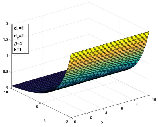
Figure 1. $u(x,t)=d_1{e}^{-\frac{2+\beta }{4+\beta }kt}+d_2{e}^{-\frac{2}{4+\beta }kt}.$

3.7. Reductions for Subcase  1.2.1.1

Equation (1) becomes

$$u_{tt}=f_1{u}^{1-\beta k_1}+\beta u^{\beta -1}{u}_x^2+u^{\beta }{u}_{xx}.$$

(44)

The generator

$${\mathcal{X}}^1=x\frac{\partial }{\partial x}+(\frac{k_1}{(k_1+1)}t+1)\frac{\partial }{\partial t}+\frac{2}{\beta (k_1+1)}u\frac{\partial }{\partial u},$$

having invariants

$$\omega =x{\left(k_{1}t+(k_1+1)\right)}^{-\frac{k_1+1}{k_1}},$$

$$u=\varphi {\left(k_{1}t+(k_1+1)\right)}^{\frac{2}{\beta k_1}}$$

transforms (44) into

$$\left({(k_1+1)}^2{\omega }^2-{\varphi }^{\beta }\right){\varphi }^{″}+\frac{2}{{\beta }^2}(2-\beta (2k_1+1)){(k_1+1)}^2\omega {\varphi }^{\prime }-\beta {\varphi }^{\beta -1}{\varphi }^{\prime 2}+\frac{4-2\beta k_1}{{\beta }^2}\varphi -f_1{\varphi }^{1-\beta k_1}=0.$$

Similarly, ${\mathcal{X}}^2$ leads to

$$(\frac{{(k_1+1)}^2}{k_1^2}{\omega }^2-{\varphi }^{\beta }){\varphi }^{″}+\frac{2}{{\beta }^2{k}^4}(2-\beta (2k_1+1)){(k_1+1)}^2\omega {\varphi }^{\prime }-\beta {\varphi }^{\beta -1}{\varphi }^{\prime 2}+\frac{4-2\beta k_1}{{\beta }^2{k}^2}\varphi -f_1{\varphi }^{1-\beta k_1}=0$$

where the similarity variables are

$$\omega =x{t}^{-\frac{k_1+1}{k_1}},$$

$$u=\varphi t^{\frac{2}{\beta k_1}}$$

Moreover, the Lie generator ${\mathcal{X}}^3$ gives the following reduced form of (44):

$$({\varphi }^{\beta }-e_1^2){\varphi }^{″}+\beta {\varphi }^{\beta -1}{\varphi }^{\prime 2}+f_1{\varphi }^{1-\beta k_1}=0.$$

Now, for ${\mathcal{X}}^4$, we have

$${\varphi }^{″}-f_1{\varphi }^{1-\beta k_1}=0,$$

by means of the invariants $\omega =t$ and $u=\varphi \left(\omega \right),$ which yields the following exact invariant solution

$$\frac{\varphi {\left(\omega \right)}^2\left(\frac{2f_1\varphi {\left(\omega \right)}^{2-\beta k_1}}{d_1(2-\beta k_1)}+1\right)F_1{\left(\frac{1}{2},\frac{1}{2-\beta k_1};1+\frac{1}{2-\beta k_1};-\frac{2f_1\varphi {\left(\omega \right)}^{2-\beta k_1}}{d_1(2-\beta k_1)}\right)}^2}{\frac{2f_1\varphi {\left(\omega \right)}^{2-\beta k_1}}{2-\beta k_1}+d_1}={(d_2+\omega )}^2.$$

3.8. Reductions for Subcase  1.2.2.1

Equation (1) in this case is

$$u_{tt}+k{u}_t=f_{1}u-4u^{-5}{u}_x^2+u^{-4}{u}_{xx}.$$

(45)

The Lie generator ${\mathcal{X}}^1$ has the similarity variables

$$\omega =ln\left(x\right)-\frac{k}{e_2}t,u=\varphi x^{-1/2},$$

that reduce (45) to the form

$$({\varphi }^{-4}-\frac{k^2}{e_2^2}){\varphi }^{″}-4{\varphi }^{-5}{\varphi }^{\prime 2}+3{\varphi }^{-4}{\varphi }^{\prime }+\frac{k^2}{e_2^2}{\varphi }^{\prime }-\frac{1}{4}{\varphi }^{-3}+f_1\varphi =0.$$

Now for ${\mathcal{X}}^2$, we have

$$({\varphi }^{-4}-\frac{k^2}{e_2^2}){\varphi }^{″}-4{\varphi }^{-5}{\varphi }^{\prime 2}+\frac{k^2}{e_2^2}{\varphi }^{\prime }+f_1\varphi =0.$$

via the similarity variables

$$\omega =x-\frac{k}{e_2}t,u=\varphi .$$

Also, for the translation in time

$${\mathcal{X}}^3=\frac{1}{k}\frac{\partial }{\partial t},$$

(45) becomes

$${\varphi }^{-4}{\varphi }^{″}-4{\varphi }^{-5}{\varphi }^{\prime 2}+f_1\varphi =0.$$

3.9. Reductions for Subcase  1.2.2.2 (C)

Equation (1) for this case is

$$u_{tt}=f_2{u}^{f_1}-4u^{-5}{u}_x^2+u^{-4}{u}_{xx}.$$

(46)

${\mathcal{X}}^1$ with the similarity variables

$$\omega =x{\left((f_1-1)t\pm (f_1+3)\right)}^{-\frac{f_1+3}{f_1-1}},$$

$$u=\varphi {\left((f_1-1)t\pm (f_1+3)\right)}^{-\frac{2}{f_1-1}},$$

converts (46) to the Ode as

$$({(3+f_1)}^2{\omega }^2-{\varphi }^{-4}){\varphi }^{″}+2{(3+f_1)}^2{\varphi }^{\prime }\omega +4{\varphi }^{-5}{\varphi }^{\prime 2}+2(f_1+1)\varphi -f_2{\varphi }^{f_1}=0.$$

For ${\mathcal{X}}^2$, we derive the following similarity transformations:

$$\omega =x{t}^{-\frac{f_1+3}{f_1-1}},$$

$$u=\varphi t^{-\frac{2}{f_1-1}},$$

which transforms (46) into

$$(\frac{{(3+f_1)}^2}{{(f_1-1)}^2}{\omega }^2-{\varphi }^{-4}){\varphi }^{″}+2\frac{{(3+f_1)}^2}{{(f_1-1)}^2}{\varphi }^{\prime }\omega +4{\varphi }^{-5}{\varphi }^{\prime 2}+2(f_1+1)\varphi -f_2{\varphi }^{f_1}=0.$$

Also, for the traveling wave symmetry generator ${\mathcal{X}}^3$, we obtain the following reduction

$$({\varphi }^{-4}{e}_2^2-1){\varphi }^{″}-4{\varphi }^{-5}{\varphi }^{\prime 2}+f_2{\varphi }^{f_1}=0.$$

Similarly, for ${\mathcal{X}}^4$, we obtain the reduction of (46) as

$${\varphi }^{-4}{\varphi }^{″}-4{\varphi }^{-5}{\varphi }^{\prime 2}+f_2{\varphi }^{f_1}=0.$$

3.10. Reductions for Subcase  2.1.1.1 (2)

In this case, (1) can be written as

$$u_{tt}=\frac{9}{4}{F}_1{u}^{-1/3}+F_{2}u-\frac{4}{3}{u}^{-7/3}{u}_x^2+u^{-4/3}{u}_{xx}.$$

(47)

The symmetry generator ${\mathcal{X}}^1$ reduces (47) to

$$({\varphi }^{-4/3}-1){\varphi }^{″}+F_2\varphi -\frac{9}{4}{F}_1{\varphi }^{-1/3}-\frac{4}{3}{\varphi }^{-7/3}{\varphi }^{\prime 2}=0,$$

where the similarity variables for this symmetry generator are

$$\omega =t-\frac{1}{\sqrt{3F_1}}ta{n}^{-1}(sinh\sqrt{3F_1}x),$$

and

$$u=\varphi {(cosh\sqrt{3F_1}x)}^{-3/2}.$$

Likewise, ${\mathcal{X}}^2$ has similarity variables $\omega =3F_1{e}_{2}x+t$ and $u=\varphi ,$ which transform (47) into

$$(9F_1^2{e}_2^2{\varphi }^{-4/3}-1){\varphi }^{″}+F_2\varphi +\frac{9}{4}{F}_1{\varphi }^{-1/3}-12F_1^2{e}_2^2{\varphi }^{-7/3}{\varphi }^{\prime 2}=0.$$

Now we consider ${\mathcal{X}}^3$, which has the respective invariants of the form

$$\omega =t-\frac{1}{\sqrt{3F_1}}{e}^{\sqrt{3F_1}x},u=\varphi e^{\frac{3\sqrt{3F_1}}{2}x},$$

and for these invariants we arrive at the following reduced differential equation:

$$({\varphi }^{-4/3}{e}_2^2-1){\varphi }^{″}+F_2\varphi -\frac{4}{3}{e}_2^2{\varphi }^{-7/3}{\varphi }^{\prime 2}=0.$$

Now for ${\mathcal{X}}^4$ we find

$$\omega =t+\frac{1}{\sqrt{3F_1}}{e}^{-\sqrt{3F_1}x},u=\varphi e^{-\frac{3\sqrt{3F_1}}{2}x},$$

which results in the same reduced differential equation given above. The reduced Ode for ${\mathcal{X}}^5$ is

$${\varphi }^{-4/3}{\varphi }^{″}+F_2\varphi -\frac{4}{3}{\varphi }^{-7/3}{\varphi }^{\prime 2}+\frac{9}{4}{F}_1{\varphi }^{-1/3}=0.$$

3.11. Reductions for Subcase  2.1.1.2 (1)

In this case, (1) takes the form

$$u_{tt}=\frac{9}{4}{F}_1{u}^{-1/3}-\frac{4}{3}{u}^{-7/3}{u}_x^2+u^{-4/3}{u}_{xx}.$$

(48)

The symmetry generator ${\mathcal{X}}^1$ reduces (48) to

$$({\varphi }^{-4/3}-1){\varphi }^{″}+F_2\varphi -\frac{9}{4}{F}_1{\varphi }^{-1/3}-\frac{4}{3}{\varphi }^{-7/3}{\varphi }^{\prime 2}-\frac{3}{4}{\varphi }^{1/3}=0,$$

where the similarity variables for this symmetry generator are

$$\omega =-\frac{1}{\sqrt{3F_1}}ta{n}^{-1}\left(e^{\sqrt{3F_1}x}\right)+ln\left(t\right),$$

and

$$u=\sqrt{3F_1}(e^{\sqrt{3F_1}x}-e^{-\sqrt{3F_1}x})+\varphi t^{3/2}.$$

For ${\mathcal{X}}^2$, the invariants are given by

$$\omega =ln\left(t\right)-\frac{1}{\sqrt{3F_1}}{e}^{\sqrt{3F_1}x},u=\varphi e^{\frac{3}{2}(\sqrt{3F_1}x+\frac{1}{\sqrt{3F_1}}{e}^{\sqrt{3F_1}x})}$$

that yields

$$({\varphi }^{-4/3}+{\omega }^2){\varphi }^{″}+{\varphi }^{-4/3}{\varphi }^{\prime }-\frac{4}{3}{\varphi }^{-7/3}{\varphi }^{\prime 2}-\frac{3}{4}{\varphi }^{1/3}=0.$$

(49)

Now for ${\mathcal{X}}^3$, the invariants

$$\omega =ln\left(t\right)+\frac{3F_1}{e_1}x,u=\varphi t^{3/2},$$

reduce (48) to

$$({\varphi }^{-4/3}-e_1^2){\varphi }^{″}-2e_1^2{\varphi }^{\prime }-\frac{3}{4}{e}_1^2\varphi -\frac{4}{3}{\varphi }^{-7/3}{\varphi }^{\prime 2}+\frac{9}{4}{F}_1{e}_1^2{\varphi }^{-1/3}=0.$$

The reduction of (48) for ${\mathcal{X}}^4$ is the same as given in (49), with respect to the following invariants:

$$\omega =ln\left(t\right)+\frac{1}{\sqrt{3F_1}}{e}^{-\sqrt{3F_1}x},u=\varphi e^{-\frac{3}{2}(\sqrt{3F_1}x+\frac{1}{\sqrt{3F_1}}{e}^{-\sqrt{3F_1}x})}.$$

The reduced differential equation for ${\mathcal{X}}^5$ is

$$({\varphi }^{-4/3}-{\omega }^2){\varphi }^{″}-\frac{3}{4}\varphi -\frac{4}{3}{\varphi }^{-7/3}{\varphi }^{\prime 2}+\frac{9}{4}{F}_1{\varphi }^{-1/3}=0,$$

subject to $\omega =xt$ and $u=\varphi t^{3/2}$.

In a like manner, for ${\mathcal{X}}^6$, the reduction of (48) is given by

$$({\varphi }^{-4/3}-1){\varphi }^{″}-\frac{9}{4}{F}_1{\varphi }^{-1/3}-\frac{4}{3}{\varphi }^{-7/3}{\varphi }^{\prime 2}=0,$$

where the similarity variables for this symmetry generator are

$$\omega =t-\frac{1}{\sqrt{3F_1}}ta{n}^{-1}(sinh\sqrt{3F_1}x),$$

and

$$u=\varphi {(cosh\sqrt{3F_1}x)}^{-3/2}.$$

Also, the Lie symmetry ${\mathcal{X}}^7$ with respective invariants

$$\omega =t-\frac{1}{\sqrt{3F_1}}{e}^{\sqrt{3F_1}x},u=\varphi e^{\frac{3\sqrt{3F_1}}{2}x},$$

gives the reduction

$$({\varphi }^{-4/3}-1){\varphi }^{″}-\frac{4}{3}{\varphi }^{-7/3}{\varphi }^{\prime 2}=0.$$

Similarly, for ${\mathcal{X}}^8$, the reduced form is

$$(9F_1^2{\varphi }^{-4/3}-1){\varphi }^{″}+\frac{9}{4}{F}_1{\varphi }^{-1/3}-12F_1^2{\varphi }^{-7/3}{\varphi }^{\prime 2}=0.$$

The reduced Ode for ${\mathcal{X}}^9$ is

$${\varphi }^{″}-\frac{9}{4}{F}_1{\varphi }^{-1/3}=0.$$

Associated to ${\mathcal{X}}^{10}$, the reduced form of (48) is given by

$$({\varphi }^{-4/3}-e_3^2){\varphi }^{″}-\frac{4}{3}{\varphi }^{-7/3}{\varphi }^{\prime 2}=0,$$

via the invariants

$$\omega =e_{3}t+\frac{1}{\sqrt{3F_1}}{e}^{-\sqrt{3F_1}x},u=\varphi e^{-\frac{3\sqrt{3F_1}}{2}x}.$$

Similarly, for ${\mathcal{X}}^{11}$, we arrive at the reduced form

$${\varphi }^{″}=0,$$

subject to the invariants

$$\omega =t,u=\varphi e^{-\frac{3\sqrt{3F_1}}{2}x}.$$

The corresponding invariant solution is

$$u(x,t)=(d_1+d_{2}t)e^{-\frac{3\sqrt{3F_1}}{2}x}.$$

Graphically, this shows exponential decay.

Figure 2 shows exponential decay in the amplitude of the wave. As x increases, the amplitude of the wave swiftly diminishes. In other words, the wave spreads linearly with time t and then diminishes exponentially as we move along the x-axis in the positive direction due to the term $e^{-\frac{3\sqrt{3F_1}}{2}x}$. This solution illustrates the behavior of the wave that spreads and grows linearly with time while also decays in amplitude with spatial distance.

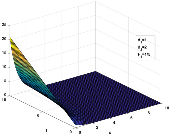
Figure 2. $u(x,t)=(d_1+d_{2}t)e^{-\frac{3\sqrt{3F_1}}{2}x}.$

The similarity variables

$$\omega =t,u=\varphi {(cosh\sqrt{3F_1}x)}^{-3/2},$$

associated with ${\mathcal{X}}^{12}$ gives the following reduction of (48):

$${\varphi }^{″}+\frac{9}{4}{F}_1{\varphi }^{-1/3}=0.$$

3.12. Reductions for Subcase  2.1.1.2 (2)

Here, (1) becomes

$$u_{tt}=F_3-\frac{4}{3}{u}^{-7/3}{u}_x^2+u^{-4/3}{u}_{xx}.$$

(50)

We begin with ${\mathcal{X}}^1$ for which the invariants

$$\omega =x^3-(t+1),$$

and

$$u=\varphi {(t+1)}^2,$$

reduce (50) to the differential equation

$$(9{\omega }^{4/3}{\varphi }^{-4/3}-{\omega }^2){\varphi }^{″}+{\varphi }^{\prime }(6{\omega }^{1/3}{\varphi }^{-4/3}-4\omega -12{\omega }^{4/3}{\varphi }^{-7/3}{\varphi }^{\prime })-2\varphi +F_3=0.$$

For ${\mathcal{X}}^2$, we obtain the same reduced Ode, as given above. However, the similarity transformations for this symmetry generator are

$$\omega =x^3-t,u=\varphi t^2.$$

Similarly, for ${\mathcal{X}}^3$, the invariants $\omega =x-e_{1}t$ and $u=\varphi \left(\omega \right),$ results in the reduction

$$({\varphi }^{-4/3}-e_1^2){\varphi }^{″}-{\omega }^{4/3}{\varphi }^{-7/3}{\varphi }^{\prime 2}-F_3=0.$$

The reduced differential equation for the translational symmetry ${\mathcal{X}}^4$ is

$${\varphi }^{″}-F_3=0,$$

subject to $\omega =t$ and $u=\varphi$. This results in the following exact solution of (50)

$$u(x,t)=d_1+d_{2}t+\frac{1}{2}{t}^2{F}_3,$$

and the graphical illustration of this solution is shown below.

Figure 3 shows the quadratic behavior of the solution that increases with time.

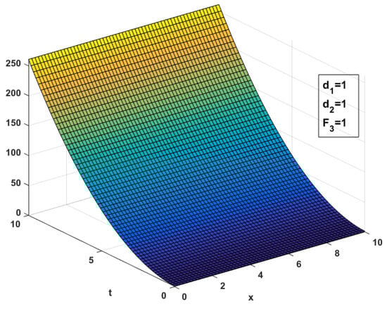
Figure 3. $u(x,t)=d_1+d_{2}t+\frac{1}{2}{t}^2{F}_3.$

3.13. Reductions for Subcase  2.1.2.1 (2)

In this case, (1) can be written as

$$u_{tt}+A{u}_t=\frac{9}{4}{F}_1{u}^{-1/3}+F_{2}u-\frac{4}{3}{u}^{-7/3}{u}_x^2+u^{-4/3}{u}_{xx}.$$

(51)

The Lie symmetry generator ${\mathcal{X}}^1$ reduces (51) to

$$({\varphi }^{-4/3}-1){\varphi }^{″}-A{\varphi }^{\prime }+F_2\varphi -\frac{9}{4}{F}_1{\varphi }^{-1/3}-\frac{4}{3}{\varphi }^{-7/3}{\varphi }^{\prime 2}=0,$$

where the similarity variables for this symmetry generator are

$$\omega =t-\frac{1}{\sqrt{3F_1}}ta{n}^{-1}(sinh\sqrt{3F_1}x),$$

and

$$u=\varphi {(cosh\sqrt{3F_1}x)}^{-3/2}.$$

The reduction of (51) for ${\mathcal{X}}^2$ is

$$(12F_1^2{e}_2^2{\varphi }^{-4/3}-A^2){\varphi }^{″}-A{\varphi }^{\prime }+F_2\varphi +\frac{9}{4}{F}_1{\varphi }^{-1/3}-12F_1^2{e}_2^2{\varphi }^{-7/3}{\varphi }^{\prime 2}=0.$$

Corresponding to ${\mathcal{X}}^3$, the invariants

$$\omega =t-\frac{1}{\sqrt{3F_1}}{e}^{\sqrt{3F_1}x},u=\varphi e^{\frac{3\sqrt{3F_1}}{2}x},$$

lead to the following reduced differential equation

$$(e_2^2{\varphi }^{-4/3}-1){\varphi }^{″}-A{\varphi }^{\prime }+F_2\varphi -\frac{4}{3}{e}_2^2{\varphi }^{-7/3}{\varphi }^{\prime 2}=0.$$

Also, ${\mathcal{X}}^4$, yields the following invariants:

$$\omega =t+\frac{1}{\sqrt{3F_1}}{e}^{-\sqrt{3F_1}x},u=\varphi e^{-\frac{3\sqrt{3F_1}}{2}x},$$

and by using these invariants we deduce the same reduced differential equation as given above.

The reduction of (51) associated to ${\mathcal{X}}^5$ is

$${\varphi }^{-4/3}{\varphi }^{″}+F_2\varphi -\frac{4}{3}{\varphi }^{-7/3}{\varphi }^{\prime 2}+\frac{9}{4}{F}_1{\varphi }^{-1/3}=0.$$

3.14. Reductions for Subcase  2.1.2.2 (1)

In this case, (1) is

$$u_{tt}+A{u}_t=\frac{9}{4}{F}_1{u}^{-1/3}-\frac{3}{16}{A}^{2}u-\frac{4}{3}{u}^{-7/3}{u}_x^2+u^{-4/3}{u}_{xx}.$$

(52)

The symmetry generator ${\mathcal{X}}^1$ reduces (52) to the Ode

$$({\varphi }^{-4/3}-1){\varphi }^{″}-A{\varphi }^{\prime }-\frac{4}{3}{\varphi }^{-7/3}{\varphi }^{\prime 2}+\frac{9}{4}{F}_1{\varphi }^{-1/3}-\frac{3}{16}{A}^2\varphi =0,$$

where the similarity variables used are

$$\omega =t-\frac{1}{\sqrt{3F_1}}{tan}^{-1}(sinh\sqrt{3F_1}x),$$

and

$$u=\varphi {(cosh\sqrt{3F_1}x)}^{-3/2}.$$

Now, ${\mathcal{X}}^2$ has the similarity variables

$$\omega =t-\frac{1}{\sqrt{3F_1}}{e}^{\sqrt{3F_1}x},u=\varphi e^{\frac{3\sqrt{3F_1}}{2}x},$$

and by using these invariants, we arrive at

$$({\varphi }^{-4/3}-1){\varphi }^{″}-A{\varphi }^{\prime }-\frac{4}{3}{\varphi }^{-7/3}{\varphi }^{\prime 2}-\frac{3}{16}{A}^2\varphi =0.$$

The similarity transformations

$$\omega =\frac{1}{e_1\sqrt{3F_1}}ln|e_1{e}^{-\sqrt{3F_1}x}+1|+t,$$

and

$$u=\varphi |{e^{-\sqrt{3F_1}x}+e_1|}^{-3/2},$$

associated with ${\mathcal{X}}^3$ transforms (52) into

$$({\varphi }^{-4/3}-1){\varphi }^{″}-A{\varphi }^{\prime }-\frac{4}{3}{\varphi }^{-7/3}{\varphi }^{\prime 2}+\frac{9}{4}{e}_1^2{F}_1{\varphi }^{-1/3}-\frac{3}{16}{A}^2\varphi =0.$$

Also, for ${\mathcal{X}}^4$, we have reduction

$$({\varphi }^{-4/3}-e_1^2){\varphi }^{″}+A{e}_1{\varphi }^{\prime }-\frac{3}{16}{A}^2\varphi -\frac{4}{3}{\varphi }^{-7/3}{\varphi }^{\prime 2}+\frac{9}{4}{F}_1{\varphi }^{-1/3}=0.$$

Similarly, for ${\mathcal{X}}^6$ the similarity variables

$$\omega =t,u=\varphi {(cosh\sqrt{3F_1}x)}^{-3/2},$$

reduce (52) to

$${\varphi }^{″}+A{\varphi }^{\prime }+\frac{9}{4}{F}_1{\varphi }^{-1/3}+\frac{3}{16}{A}^2\varphi =0.$$

For ${\mathcal{X}}^7$, we obtain the reduction of (52)

$${\varphi }^{″}+A{\varphi }^{\prime }+\frac{3}{16}{A}^2\varphi =0,$$

subject to

$$\omega =t,u=\varphi e^{-\frac{3\sqrt{3F_1}}{2}x}.$$

This reduced differential equation yields the following exact solution of (52):

$$u(x,t)=e^{-\frac{3\sqrt{3F_1}}{2}x}(d_1{e}^{-\frac{3A}{4}t}+d_2{e}^{-\frac{A}{4}t}).$$

Graphically, we have the following representation.

Figure 4 shows the diminishing behavior of the wave in both space and time. The combination of the exponential terms creates a solution that represents temporal and spatial decay. The graphs shows exponential decay as we move away from the origin. Moreover, the presence of the damping term A causes faster decay. The wave initially starts with the smaller amplitude and oscillations, but decays exponentially as it moves in both space and time. It can be seen from graphs that the wave decays with the increase in time and its oscillations become smaller and smaller.

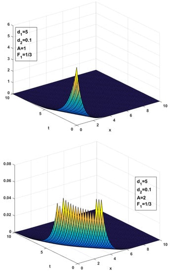
Figure 4. $u(x,t)=e^{-\frac{3\sqrt{3F_1}}{2}x}(d_1{e}^{-\frac{3A}{4}t}+d_2{e}^{-\frac{A}{4}t}).$

The similarity variables

$$\omega =x-\frac{2}{A}{e}^{\frac{A}{2}t},u=\varphi e^{-\frac{3A}{4}t},$$

associated with ${\mathcal{X}}^8$ give

$$({\varphi }^{-4/3}-1){\varphi }^{″}-\frac{4}{3}{\varphi }^{-7/3}{\varphi }^{\prime 2}+\frac{9}{4}{F}_1{\varphi }^{-1/3}=0.$$

For ${\mathcal{X}}^{10}$, the similarity variables

$$\omega =x,u=\varphi e^{-\frac{3A}{4}t},$$

reduce (52) to the Ode

$${\varphi }^{-4/3}{\varphi }^{″}-\frac{4}{3}{\varphi }^{-7/3}{\varphi }^{\prime 2}+\frac{9}{4}{F}_1{\varphi }^{-1/3}=0.$$

The symmetry generator ${\mathcal{X}}^{11}$ results in the reduction

$${\varphi }^{-4/3}{\varphi }^{″}+A{\varphi }^{\prime }-\frac{9}{4}{F}_1{e}_1^2{\varphi }^{-1/3}+\frac{3}{16}{A}^2\varphi =0,$$

subject to

$$\omega =t,u=\varphi {(e^{-\sqrt{3F_1}x}+e_1)}^{-3/2}.$$

In a like manner, ${\mathcal{X}}^{12}$ yields

$${\varphi }^{″}+A{\varphi }^{\prime }-\frac{9}{4}{F}_1{\varphi }^{-1/3}+\frac{3}{16}{A}^2\varphi =0.$$

3.15. Reductions for Subcase  2.2.1

Equation (1) in this respect takes the form

$$u_{tt}+\frac{1}{k+1}{k}_1{u}^{k+1}{u}_t=F_2{u}^{2k+3}-\frac{4}{3}{u}^{-7/3}{u}_x^2+u^{-4/3}{u}_{xx}.$$

(53)

For generator ${\mathcal{X}}^1$, we obtain the reduced form of (53),

$$\begin{array}{c}\left({\varphi }^{-4/3}-{(3k+5)}^2{\omega }^2\right){\varphi }^{″}+(3k+5)\omega {\varphi }^{\prime }\left(\frac{1}{k+1}{k}_1{\varphi }^{k+1}-3(3k+5)(6k+11)\right)-\hfill \\ \hfill \frac{4}{3}{\varphi }^{-7/3}{\varphi }^{\prime 2}+F_2{\varphi }^{2k+3}-(9k+18)\varphi +\frac{3}{k+2}{k}_1{\varphi }^{k+2}=0,\end{array}$$

where the invariants associated with this generator are

$$\omega =x{\left(\left(3\right(k+1)t+(3k+5)\right)}^{-\frac{3k+5}{3(k+1)}},$$

$$u=\varphi {\left(3(k+1)t+(3k+5)\right)}^{-\frac{1}{k+1}}.$$

Corresponding to ${\mathcal{X}}^2$, the invariants are

$$\omega =x{t}^{-\frac{3k+5}{3(k+1)}},u=\varphi t^{-\frac{1}{k+1}},$$

which yield the Ode

$$\begin{array}{c}({\varphi }^{-4/3}-\frac{{(3k+5)}^2}{{(3k+3)}^2}{\omega }^2){\varphi }^{″}+\frac{(3k+5)}{(3k+3)}\omega {\varphi }^{\prime }\left(\frac{1}{k+1}{k}_1{\varphi }^{k+1}-\frac{(3k+5)}{(3k+3)}(6k+8)\right)-\hfill \\ \hfill \frac{4}{3}{\varphi }^{-7/3}{\varphi }^{\prime 2}+F_2{\varphi }^{2k+3}-\frac{(k+2)}{{(k+1)}^2}\varphi +\frac{1}{k+1}{k}_1{\varphi }^{k+2}=0.\end{array}$$

Now, we consider ${\mathcal{X}}^3$, which reduce (53) to the Ode

$$({\varphi }^{-4/3}-e_1^2){\varphi }^{″}+\frac{k_1}{k+1}{e}_1{\varphi }^{k+1}{\varphi }^{\prime }-\frac{4}{3}{\varphi }^{-7/3}{\varphi }^{\prime 2}+F_2{\varphi }^{2k+3}=0,$$

and this gives the traveling wave solution.

The symmetry generator ${\mathcal{X}}^4$ gives the reduction

$${\varphi }^{″}+\frac{k_1}{k+1}{\varphi }^{k+1}{\varphi }^{\prime }-F_2{\varphi }^{2k+3}=0.$$

3.16. Reductions for Subcase  2.2.1.1

Equation (1) in this case becomes

$$u_{tt}+(-\frac{3}{2}{k}_1{u}^{-2/3}+k_2)u_t=\frac{9}{8}{k}_1{k}_2{u}^{1/3}-\frac{3}{16}{k}_2^{2}u+f_1{u}^{-1/3}-\frac{4}{3}{u}^{-7/3}{u}_x^2+u^{-4/3}{u}_{xx}.$$

(54)

The similarity variables associated with ${\mathcal{X}}^1$ are

$$\omega =x-\frac{k_2}{2}{e}_{1}t,u=\varphi \left(\omega \right).$$

Using these, we reduce (54) to the Ode

$$\begin{array}{c}({\varphi }^{-4/3}-\frac{k_2^2}{4}{e}_1^2){\varphi }^{″}+{\varphi }^{\prime }(\frac{k_2^2}{2}{e}_1-\frac{3}{4}{e}_1{k}_1{k}_2{\varphi }^{-2/3})-\hfill \\ \hfill \hspace{1em}\hspace{1em}\hspace{1em}\hspace{1em}\hspace{1em}\hspace{1em}\hspace{1em}\hspace{1em}\frac{4}{3}{\varphi }^{-7/3}{\varphi }^{\prime 2}+f_1{\varphi }^{-1/3}+\frac{9}{8}{k}_1{k}_2{\varphi }^{1/3}-\frac{3}{16}{k}_2^2\varphi =0.\end{array}$$

Similarly, for ${\mathcal{X}}^2$, we obtain

$$\left({\varphi }^{-4/3}-1\right){\varphi }^{″}-\frac{3}{2}{k}_1{\varphi }^{-2/3}{\varphi }^{\prime }-\frac{4}{3}{\varphi }^{-7/3}{\varphi }^{\prime 2}+f_1{\varphi }^{-1/3}=0,$$

with respect to the invariants

$$\omega =x-\frac{2}{k_2}{e}^{\frac{k_2}{2}t},u=\varphi e^{-\frac{3k_2}{4}t}.$$

Now, we take ${\mathcal{X}}^3$, which reduces (54) to

$${\varphi }^{″}-\frac{3}{2}{k}_1{\varphi }^{-2/3}{\varphi }^{\prime }+k_2{\varphi }^{\prime }+\frac{3}{16}{k}_2^2\varphi -\frac{9}{8}{k}_1{k}_2{\varphi }^{1/3}-f_1{\varphi }^{-1/3}=0.$$

3.17. Reductions for Subcase  2.2.1.1.1

In this case, we have following form of Equation (1):

$$u_{tt}-\frac{3}{2}{k}_1{u}^{-2/3}{u}_t=f_1{u}^{-1/3}-\frac{4}{3}{u}^{-7/3}{u}_x^2+u^{-4/3}{u}_{xx}.$$

(55)

Analogous to ${\mathcal{X}}^1$, the reduced Ode is

$$(\frac{1}{e_1^2}{\varphi }^{-4/3}-1){\varphi }^{″}+{\varphi }^{\prime }(\frac{3}{2}{k}_1{\varphi }^{-2/3}-2)-\frac{4}{3e_1^2}{\varphi }^{-7/3}{\varphi }^{\prime 2}+f_1{\varphi }^{-1/3}+\frac{9}{4}{k}_1{\varphi }^{1/3}-\frac{3}{4}\varphi =0,$$

with respect to the similarity variables

$$\omega =ln\left(t\right)-\frac{1}{e_1}x,u=\varphi t^{3/2}.$$

Similarly, for ${\mathcal{X}}^2$, we have

$$\left({\varphi }^{-4/3}-1\right){\varphi }^{″}-\frac{3}{2}{k}_1{\varphi }^{-2/3}{\varphi }^{\prime }-\frac{4}{3}{\varphi }^{-7/3}{\varphi }^{\prime 2}+f_1{\varphi }^{-1/3}=0,$$

with respect to the invariants

$$\omega =x-\frac{2}{k_2}{e}^{\frac{k_2}{2}t},u=\varphi e^{-\frac{3k_2}{4}t}.$$

Now consider ${\mathcal{X}}^3$, which reduces (55) to the ordinary differential equation

$${\varphi }^{″}-\frac{3}{2}{k}_1{\varphi }^{-2/3}{\varphi }^{\prime }-f_1{\varphi }^{-1/3}=0.$$

3.18. Reductions for Subcase  3.1.1

In this case, we have

$$u_{tt}=f_1{u}^{\sigma /3}-\frac{4}{3}{u}^{-7/3}{u}_x^2+u^{-4/3}{u}_{xx}.$$

(56)

The Lie symmetry ${\mathcal{X}}^1$ with the respective invariants

$$\omega =x{\left((\sigma -3)t\pm (\sigma +1)\right)}^{-\frac{\sigma +1}{(\sigma -3)}},$$

$$u=\varphi {\left((\sigma -3)t\pm (\sigma +1)\right)}^{-\frac{6}{(\sigma -3)}},$$

transforms (56) into Ode

$$\begin{array}{c}\left({\varphi }^{-4/3}-{(\sigma +1)}^2{\omega }^2\right){\varphi }^{″}-2(\sigma +1)(\sigma +5)\omega {\varphi }^{\prime }-\hfill \\ \hfill \hspace{1em}\hspace{1em}\hspace{1em}\hspace{1em}\hspace{1em}\hspace{1em}\hspace{1em}\hspace{1em}\hspace{1em}\hspace{1em}\hspace{1em}\hspace{1em}\hspace{1em}\hspace{1em}\hspace{1em}\frac{4}{3}{\varphi }^{-7/3}{\varphi }^{\prime 2}+f_1{\varphi }^{\sigma /3}-6(\sigma +3)\varphi =0.\end{array}$$

For ${\mathcal{X}}^2$, we have

$$\begin{array}{c}({\varphi }^{-4/3}-\frac{{(\sigma +1)}^2}{{(\sigma -3)}^2}{\omega }^2){\varphi }^{″}-\frac{2(\sigma +1)}{{(\sigma -3)}^2}(\sigma +5)\omega {\varphi }^{\prime }-\hfill \\ \hfill \hspace{1em}\hspace{1em}\hspace{1em}\hspace{1em}\hspace{1em}\hspace{1em}\hspace{1em}\hspace{1em}\hspace{1em}\hspace{1em}\hspace{1em}\hspace{1em}\hspace{1em}\hspace{1em}\hspace{1em}\frac{4}{3}{\varphi }^{-7/3}{\varphi }^{\prime 2}+f_1{\varphi }^{\sigma /3}-6\frac{(\sigma +3)}{{(\sigma -3)}^2}\varphi =0.\end{array}$$

Now ${\mathcal{X}}^3$ reduces (56) to the differential equation

$$\left({\varphi }^{-4/3}{e}_2^2-1\right){\varphi }^{″}-\frac{4}{3}{\varphi }^{-7/3}{\varphi }^{\prime 2}+f_1{\varphi }^{\sigma /3}=0.$$

Also, for the translation in time ${\mathcal{X}}^4$, we obtain

$${\varphi }^{-4/3}{\varphi }^{″}-\frac{4}{3}{\varphi }^{-7/3}{\varphi }^{\prime 2}+f_1{\varphi }^{\sigma /3}=0.$$

3.19. Reductions for Subcase  3.1.1 (1)

Equation (1) in this subcase is

$$u_{tt}=f_1{u}^{-1/3}-\frac{4}{3}{u}^{-7/3}{u}_x^2+u^{-4/3}{u}_{xx}.$$

(57)

Corresponding to ${\mathcal{X}}^1$, the reduction of (57) is given by

$$(\frac{1}{e_1^2}{\varphi }^{-4/3}-1){\varphi }^{″}-2{\varphi }^{\prime }-\frac{4}{3e_1^2}{\varphi }^{-7/3}{\varphi }^{\prime 2}+f_1{\varphi }^{-1/3}-\frac{3}{4}\varphi =0.$$

For ${\mathcal{X}}^2$, we have

$$\left({\varphi }^{-4/3}-e_1^2\right){\varphi }^{″}-\frac{4}{3}{\varphi }^{-7/3}{\varphi }^{\prime 2}+f_1{\varphi }^{-1/3}=0.$$

Also, for translation in x, that is, ${\mathcal{X}}^3$, we obtain

$${\varphi }^{″}-f_1{\varphi }^{-1/3}=0.$$

This leads to the following exact solution:

$$\frac{(3d_1\sqrt{f_1}\sqrt[3]{\varphi \left(\omega \right)}-d_1^{3/2}\sqrt{\frac{9f_1\varphi {\left(\omega \right)}^{2/3}}{d_1}+3}{sinh}^{-1}\left(\frac{\sqrt{3f_1}\sqrt[3]{\varphi \left(\omega \right)}}{\sqrt{d_1}}\right)+9f_1^{3/2}\varphi \left(\omega \right){)}^2}{36f_1^3(d_1+3f_1\varphi {\left(\omega \right)}^{2/3})}={(d_2+\omega )}^2$$

3.20. Reductions for Subcase  3.1.1 (2)

Equation (1) in this case is

$$u_{tt}=f_{1}u-\frac{4}{3}{u}^{-7/3}{u}_x^2+u^{-4/3}{u}_{xx}.$$

(58)

The symmetry generator ${\mathcal{X}}^1$ yields the reduction of (58)

$$({\varphi }^{-4/3}-\frac{1}{e_2^2}){\varphi }^{″}-2{\varphi }^{\prime }-\frac{4}{3}{\varphi }^{-7/3}{\varphi }^{\prime 2}+f_1\varphi +\frac{3}{4}{\varphi }^{-1/3}=0.$$

Similarly for ${\mathcal{X}}^2$, we obtain

$$\left({\varphi }^{-4/3}{e}_2^2-1\right){\varphi }^{″}-\frac{4}{3}{\varphi }^{-7/3}{\varphi }^{\prime 2}+f_1\varphi =0.$$

Also, for the translation in time, ${\mathcal{X}}^3$, we find

$${\varphi }^{-4/3}{\varphi }^{″}-\frac{4}{3}{\varphi }^{-7/3}{\varphi }^{\prime 2}+f_1\varphi =0.$$

4. Conservation Laws

Conservation laws, central to symmetry analysis, arise as a result of Noether’s theorem, which connects continuous symmetries and conserved quantities of a system. In the framework of Noether’s theorem, a conservation law is a divergence expression, indicating that certain physical quantities remain conserved due to the symmetries embedded in a system described by differential equations. The study of these conserved quantities, inter alia, are useful for double reduction, linearization of Pdes and determining nonlocal symmetries of differential equations.

In this study, we find conservation laws via the partial Lagrangian approach due to Mahomed and Kara [10]. A partial Lagrangian of Equation (1) is of the form

$$\mathcal{L}=\frac{1}{2}{u}_t^2-\frac{1}{2}{u}^{\beta }{u}_x^2+\int f\left(u\right)du,$$

(59)

where

$$\frac{\partial \mathcal{L}}{\partial u}=\alpha \left(u\right)u_t-\frac{1}{2}\beta u^{\beta -1}{u}_x^2.$$

The operator in Equation (3) associated with the Lagrangian (59) is called the partial Noether operator of Equation (1) if the condition below is satisfied, viz.

$${\chi }^{\left[1\right]}\mathcal{L}+({\mathcal{D}}_t{\xi }^1+{\mathcal{D}}_x{\xi }^2)\mathcal{L}=\mathcal{W}\frac{\partial \mathcal{L}}{\partial u}+{\mathcal{D}}_t{\mathcal{B}}^1+{\mathcal{D}}_x{\mathcal{B}}^2,$$

(60)

where,

$$\mathcal{W}=\phi -{\xi }^1{u}_t-{\xi }^2{u}_x,$$

${\mathcal{B}}^1\&{\mathcal{B}}^2$ are gauge terms depending on $(x,t,u)$. From Equation (60), we arrive at the following set of determining equations:

$$\begin{array}{cc}\hfill {\xi }^1=0,{\xi }^2=0,{\zeta }_u& =0,\hfill \end{array}$$

(61)

$$\begin{array}{cc}\hfill {\zeta }_x{u}^{\beta }+{\mathcal{B}}_u^2& =0,\hfill \end{array}$$

(62)

$$\begin{array}{cc}\hfill {\zeta }_t-\zeta \alpha \left(u\right)-{\mathcal{B}}_u^1& =0,\hfill \end{array}$$

(63)

$$\begin{array}{cc}\hfill \zeta f\left(u\right)-{\mathcal{B}}_t^1-{\mathcal{B}}_x^2& =0.\hfill \end{array}$$

(64)

From Equation (61), we have

$$\zeta =\mathcal{A}(t,x).$$

(65)

Also, Equation (63) gives

$${\mathcal{B}}^1={\mathcal{A}}_{t}u-\mathcal{A}\int \alpha \left(u\right)du+\mathcal{G}(t,x).$$

(66)

Moreover, from Equation (62), we determine

$${\mathcal{B}}^2=-\frac{1}{\beta +1}{\mathcal{A}}_x{u}^{\beta +1}+\mathcal{F}(t,x),$$

(67)

with the conserved vectors arising as

$${\mathcal{T}}^t={\mathcal{B}}^1-\mathcal{A}{u}_t,$$

$${\mathcal{T}}^x={\mathcal{B}}^2+\mathcal{A}{u}^{\beta }{u}_x,$$

subject to the condition

$$\mathcal{A}f\left(u\right)={\mathcal{A}}_{tt}u-{\mathcal{A}}_t\int \alpha \left(u\right)du+{\mathcal{G}}_t-\frac{1}{\beta +1}{\mathcal{A}}_{xx}{u}^{\beta +1}+{\mathcal{F}}_x.$$

(68)

Now we consider different cases for arbitrary $\alpha \left(u\right)$ and $f\left(u\right).$

Case 1: 

If $f\left(u\right)$, $\alpha \left(u\right)$, $u^{\beta +1}$ and u are not related, then

$$\begin{array}{cc}\hfill \mathcal{A}& =0,\hfill \\ \hfill {\mathcal{H}}_x^1+{\mathcal{H}}_t^2& =0.\hfill \end{array}$$

So, no operators are obtained in this case.

Case 2: 

If $f\left(u\right)=0$.

Subcase 2.1: 

If $\alpha \left(u\right)$ is arbitrary function of u provided $\alpha \left(u\right)\ne u^{\beta }$, the conserved vectors in this case are

$$\begin{array}{cc}\hfill {\mathcal{T}}^t& =-({\mathcal{A}}_1+{\mathcal{A}}_{2}x)\int \alpha \left(u\right)du+\mathcal{G}-({\mathcal{A}}_1+{\mathcal{A}}_{2}x)u_t,\hfill \\ \hfill {\mathcal{T}}^x& =-\frac{1}{\beta +1}{\mathcal{A}}_2{u}^{\beta +1}+\mathcal{F}+({\mathcal{A}}_1+{\mathcal{A}}_{2}x)u^{\beta }{u}_x.\hfill \end{array}$$

Here, ${\mathcal{A}}_1$ and ${\mathcal{A}}_2$ are the constants.

So, we end up having the following conserved vectors:

$$({\mathcal{T}}_1^t,{\mathcal{T}}_1^x)=\left(-\int \alpha \left(u\right)du+\mathcal{G}-u_t,u^{\beta }{u}_x+\mathcal{F}\right),$$

$$({\mathcal{T}}_2^t,{\mathcal{T}}_2^x)=\left(-x\int \alpha \left(u\right)du+\mathcal{G}-x{u}_t,x{u}^{\beta }{u}_x+\mathcal{F}-\frac{1}{\beta +1}{u}^{\beta +1}\right).$$

Subcase 2.2: If $\alpha \left(u\right)=u^{\beta }$, the conserved vectors in this case are

$$\begin{array}{cc}\hfill {\mathcal{T}}^t& =-2{\mathcal{A}}_{3}u-({\mathcal{A}}_1+{\mathcal{A}}_{2}x+{\mathcal{A}}_3(-2t+x^2))(\frac{1}{\beta +1}{u}^{\beta +1}+u_t)+\mathcal{G},\hfill \\ \hfill {\mathcal{T}}^x& =-\frac{1}{\beta +1}({\mathcal{A}}_2+2{\mathcal{A}}_{3}x)u^{\beta +1}+\mathcal{F}+({\mathcal{A}}_1+{\mathcal{A}}_{2}x+{\mathcal{A}}_3(-2t+x^2))u^{\beta }{u}_x.\hfill \end{array}$$

Herein ${\mathcal{A}}_1$, ${\mathcal{A}}_2$ and ${\mathcal{A}}_3$ are constants.

Subcase 2.3: 

If $\alpha \left(u\right)=\alpha$ is constant, the conserved vectors are

$$\begin{array}{cc}\hfill {\mathcal{T}}^t& =-({\mathcal{A}}_1+{\mathcal{A}}_{2}x)\int \alpha \left(u\right)du+\mathcal{G}-({\mathcal{A}}_1+{\mathcal{A}}_{2}x)u_t,\hfill \\ \hfill {\mathcal{T}}^x& =-\frac{1}{\beta +1}{\mathcal{A}}_2{u}^{\beta +1}+\mathcal{F}+({\mathcal{A}}_1+{\mathcal{A}}_{2}x)u^{\beta }{u}_x,\hfill \end{array}$$

where ${\mathcal{A}}_1$ and ${\mathcal{A}}_2$ are constants.

Case 3: 

If $f\left(u\right)=f_1+f_{2}u$ and $\alpha \left(u\right)$ is not linear in u, then

$$\begin{array}{cc}\hfill \mathcal{A}& =0,\hfill \\ \hfill {\mathcal{H}}_x^1+{\mathcal{H}}_t^2& =0.\hfill \end{array}$$

No operators arise in this case.

Case 4: 

If $f\left(u\right)=f_1+f_2{u}^{\beta +1}$ and $\alpha \left(u\right)$ is not linear in u, then

For $f_2>0$, the following components are obtained:

$${\mathcal{T}}^t=-({\mathcal{A}}_{1}cos\sqrt{f_2(\beta +1)}x+{\mathcal{A}}_{2}sin\sqrt{f_2(\beta +1)}x)(\int \alpha \left(u\right)du+u_t)+\mathcal{G},$$

$$\begin{array}{c}{\mathcal{T}}^x=({\mathcal{A}}_{1}sin\sqrt{f_2(\beta +1)}x-{\mathcal{A}}_{2}cos\sqrt{f_2(\beta +1)}x)[\frac{1}{\beta +1}\sqrt{f_2(\beta +1)}{u}^{\beta +1}+\hfill \\ \hfill \frac{f_1}{\sqrt{f_2(\beta +1)}}]+({\mathcal{A}}_{1}cos\sqrt{f_2(\beta +1)}x+{\mathcal{A}}_{2}sin\sqrt{f_2(\beta +1)}x)u^{\beta }{u}_x,\end{array}$$

where ${\mathcal{A}}_1$ and ${\mathcal{A}}_2$ are constants. Now, for $f_2<0$, we deduce the following components of conserved quantities:

$${\mathcal{T}}^t=-({\mathcal{A}}_1{\mathrm{e}}^{\sqrt{f_2(\beta +1)}x}+{\mathcal{A}}_2{\mathrm{e}}^{-\sqrt{f_2(\beta +1)}x})(\int \alpha \left(u\right)du+u_t)+\mathcal{G},$$

$$\begin{array}{c}{\mathcal{T}}^x={\mathcal{A}}_1{\mathrm{e}}^{\sqrt{f_2(\beta +1)}x}[-\frac{\sqrt{f_2(\beta +1)}}{\beta +1}{u}^{\beta +1}+\frac{f_1}{\sqrt{f_2(\beta +1)}}+u_x{u}^{\beta }]+\hfill \\ \hfill {\mathcal{A}}_2{\mathrm{e}}^{-\sqrt{f_2(\beta +1)x}}[\frac{\sqrt{f_2(\beta +1)}}{\beta +1}{u}^{\beta +1}-\frac{f_1}{\sqrt{f_2(\beta +1)}}+u_x{u}^{\beta }],\end{array}$$

where ${\mathcal{A}}_1$ and ${\mathcal{A}}_2$ are constants. Hence, for constants ${\mathcal{A}}_1$ and ${\mathcal{A}}_2$, there are two independent conserved quantities, i.e., ${\mathcal{T}}_1=({\mathcal{T}}_1^t,{\mathcal{T}}_1^x)$ and ${\mathcal{T}}_2=({\mathcal{T}}_2^t,{\mathcal{T}}_2^x)$ for (${\mathcal{A}}_1=1,{\mathcal{A}}_2=0$) and (${\mathcal{A}}_2=1,{\mathcal{A}}_1=0$), respectively.

Case 5: 

If $f\left(u\right)=k_1\int \alpha \left(u\right)du$.

In this case, we determine the conserved components as

$${\mathcal{T}}^t=-{\mathcal{A}}_1\left(k_{1}u+(1-k_{1}t)(\int \alpha \left(u\right)du+u_t)\right)+\mathcal{G},$$

$${\mathcal{T}}^x={\mathcal{A}}_1(1-k_{1}t)u^{\beta }{u}_x+\mathcal{F}.$$

Case 6: If $\alpha \left(u\right)=\alpha$ is constant.

Here, we have different subcases.

Subcase 6.1: 

If $f\left(u\right)=f$ is a constant, the conserved vectors in this case are

$$\begin{array}{cc}\hfill {\mathcal{T}}^t& =-({\mathcal{A}}_1+{\mathcal{A}}_{2}x)\int \alpha \left(u\right)du+\mathcal{G}-({\mathcal{A}}_1+{\mathcal{A}}_{2}x)u_t,\hfill \\ \hfill {\mathcal{T}}^x& =-\frac{1}{\beta +1}{\mathcal{A}}_2{u}^{\beta +1}+\mathcal{F}+({\mathcal{A}}_1+{\mathcal{A}}_{2}x)u^{\beta }{u}_x,\hfill \end{array}$$

where ${\mathcal{A}}_1$ and ${\mathcal{A}}_2$ are constants.

Subcase 6.2: 

If $f\left(u\right)=k_1{u}^{\beta +1}$, the conserved vectors are

$${\mathcal{T}}^t=-cos\sqrt{k_1(\beta +1)}x[{\mathcal{A}}_3(\alpha u+u_t)+{\mathcal{A}}_1\frac{{\mathrm{e}}^{\alpha t}}{\alpha }]-sin\sqrt{k_1(\beta +1)}x[{\mathcal{A}}_4(\alpha u+u_t)+{\mathcal{A}}_2\frac{{\mathrm{e}}^{\alpha t}}{\alpha }]+\mathcal{G},$$

$$\begin{array}{c}\hfill {\mathcal{T}}^x=cos\sqrt{k_1(\beta +1)}x[\frac{\sqrt{k_1(\beta +1)}}{\beta +1}({\mathcal{A}}_4+{\mathcal{A}}_2\frac{{\mathrm{e}}^{\alpha t}}{\alpha })u^{\beta +1}+({\mathcal{A}}_3+{\mathcal{A}}_1\frac{{\mathrm{e}}^{\alpha t}}{\alpha })u^{\beta }{u}_x]+\\ \hfill sin\sqrt{k_1(\beta +1)}x[\frac{\sqrt{k_1(\beta +1)}}{\beta +1}({\mathcal{A}}_3+{\mathcal{A}}_1\frac{{\mathrm{e}}^{\alpha t}}{\alpha })u^{\beta +1}+({\mathcal{A}}_4+{\mathcal{A}}_2\frac{{\mathrm{e}}^{\alpha t}}{\alpha })u^{\beta }{u}_x]+\mathcal{F}.\end{array}$$

5. Conclusions

The complete Lie point symmetry classification of (1) was performed for the arbitrary smooth functions $\alpha \left(u\right)$ and $f\left(u\right)$. All possible choices for the extension of the principal Lie symmetry algebra were covered. The optimal system of one dimensional subalgebras was obtained for each case as arising from the symmetry Lie group classification. Reductions for all the cases were performed using the Lie subalgebras. Also, exact invariant solutions and their graphs were presented in some cases. Moreover, we have also studied the conservation laws via the partial Lagrangian approach. All the possible cases were discussed in order to find the conserved vectors of (1).

References

- Ovsiannikov, L.V. Group Analysis of Differential Equations; Academic Press: New York, NY, USA, 1982. [Google Scholar]
- Bluman, G.W.; Kumei, S. Symmetries and Differential Equations; Applied Mathematical Sciences; Springer: New York, NY, USA, 1989; Volume 81. [Google Scholar]
- Bluman, G.W.; Cheviakov, A.F.; Anco, S.C. Applications of Symmetry Methods to Partial Differential Equations; Springer: New York, NY, USA, 2010. [Google Scholar]
- Olver, P.J. Applications of Lie Groups to Differential Equations; Springer Science & Business Media: Berlin/Heidelberg, Germany, 1993; Volume 107. [Google Scholar]
- Ibragimov, N.H. CRC Handbook of Lie Group Analysis of Differential Equations; CRC Press: Boca Raton, FL, USA, 1995; Volume 3. [Google Scholar]
- Ames, W.F.; Lohner, R.J.; Adams, E. Group properties of utt = [f(u)ux]x. Int. J. Non-Linear Mech. 1981, 16, 439–447. [Google Scholar] [CrossRef]
- Azad, H.; Mustafa, M.T.; Ziad, M. Group classification, optimal system and optimal reductions of a class of Klein Gordon equations. Commun. Nonlinear Sci. Numer. Simul. 2010, 15, 1132–1147. [Google Scholar] [CrossRef]
- Bokhari, A.H.; Al-Dweik, A.Y.; Zaman, F.D.; Kara, A.H.; Mahomed, F.M. Generalization of the double reduction theory. Nonlinear Anal. Real World Appl. 2010, 11, 3763–3769. [Google Scholar] [CrossRef]
- Khalique, C.M.; Mahomed, F.M. Conservation laws for equations related to soil water equations. Math. Probl. Eng. 2005, 2005, 141–150. [Google Scholar] [CrossRef]
- Kara, A.H.; Mahomed, F.M. Noether-type symmetries and conservation laws via partial Lagrangians. Nonlinear Dyn. 2006, 45, 367–383. [Google Scholar] [CrossRef]
- Noether, A.E. Invariante variations probleme. Nachr. Akad. Wiss. Göttingen Math. Phys. KI. II 1991, 1, 186–207, English Translation in Transp. Theory Stat. Phys. 1991, 1, 186–207. [Google Scholar] [CrossRef]
- Anco, S.C.; Bluman, G. Direct Construction Method for Conservation laws of Partial Differential Equations Part I: Examples of Conservation law Classifications. Eur. J. Appl. Math. 2002, 13, 545–566. [Google Scholar] [CrossRef]
- Tian, S.F.; Xu, M.J.; Zhang, T.T. A symmetry-preserving difference scheme and analytical solutions of a generalized higher-order beam equation. Proc. R. Soc. A 2021, 477, 20210455. [Google Scholar] [CrossRef]
- Tian, S.F. Lie symmetry analysis, conservation laws and solitary wave solutions to a fourth-order nonlinear generalized Boussinesq water wave equation. Appl. Math. Lett. 2020, 100, 106056. [Google Scholar] [CrossRef]
- Mao, J.; Tian, S.F.; Zhang, T.; Yan, X.J. Lie symmetry analysis, conservation laws and analytical solutions for chiral nonlinear Schrödinger equation in (2 + 1)-dimensions. Nonlinear Anal. Model. Control 2020, 25, 358–377. [Google Scholar] [CrossRef]
- Feng, L.L.; Tian, S.F.; Zhang, T. Bäcklund transformations, nonlocal symmetries and soliton–cnoidal interaction solutions of the (2 + 1)-dimensional Boussinesq equation. Bull. Malays. Math. Sci. Soc. 2020, 43, 141–155. [Google Scholar] [CrossRef]
Disclaimer/Publisher’s Note: The statements, opinions and data contained in all publications are solely those of the individual author(s) and contributor(s) and not of MDPI and/or the editor(s). MDPI and/or the editor(s) disclaim responsibility for any injury to people or property resulting from any ideas, methods, instructions or products referred to in the content. |
© 2023 by the authors. Licensee MDPI, Basel, Switzerland. This article is an open access article distributed under the terms and conditions of the Creative Commons Attribution (CC BY) license (https://creativecommons.org/licenses/by/4.0/).