Fuzzy Grey Prediction-Based Particle Filter for Object Tracking

Abstract

A particle filter is a powerful tool for object tracking based on sequential Monte Carlo methods under a Bayesian estimation framework. A major challenge for a particle filter in object tracking is how to allocate particles to a high-probability density area. A particle filter does not take into account the historical prior information on the generation of the proposal distribution and, thus, it cannot approximate posterior density well. Therefore, a new fuzzy grey prediction-based particle filter (called FuzzyGP-PF) for object tracking is proposed in this paper. First, a new prediction model which was based on fuzzy mathematics theory and grey system theory was established, coined the Fuzzy-Grey-Prediction (FGP) model. Then, the history state sequence is utilized as prior information to predict and sample a part of particles for generating the proposal distribution in the particle filter. Simulations are conducted in the context of two typical maneuvering motion scenarios and the results indicate that the proposed FuzzyGP-PF algorithm can exhibit better overall performance in object tracking.

1. Introduction

Object tracking has become a very important research topic for many years since it can be used in many applications [1,2]. We can find a variety of approaches for object tracking in related literature [3,4,5]. For object tracking problems with linear or Gaussian system models, the Kalman filter (KF) can be applied to obtain optimal solutions [6]. For problems with nonlinear system models, many nonlinear filtering methods have been proposed, such as the extended Kalman filter (EKF) [7,8] and unscented Kalman filter (UKF) [9,10], which are usually implemented to provide Gaussian approximation to the posterior probability density function in the state space. In recent years, the particle filter [11] has attracted a lot of researchers’ attention. A particle filter is a powerful tool for object tracking based on sequential Monte Carlo methods under a Bayesian estimation framework [12]. The core of particle filter is to represent the probability density of object state by a set of random samples with their associated weights and how to allocate particles to a high-probability density area. Due to this sample-based method, particle filters are able to represent a variety of complex probability densities distribution with nonlinear and non-Gaussian dynamic systems. Thus, particle filters have been applied with great success to a variety of object tracking problems [13,14].

However, a standard particle filter (SPF) is not always satisfactory which may confront the particle degeneracy [15]. That is to say, all but a few particles have negligible weights after a few iterations. Consequently, a large amount of computational efforts is devoted to updating particles whose contribution to the approximation to posterior probability density function is almost zero. For many years, much attention has been paid to solve this problem of particle degeneration. Some novel strategies were proposed to solve this problem, and many improved variants of SPF were presented. An important strategy to overcome this problem is to design better proposal distributions. One such approach is the auxiliary particle filter (APF) [16] which improves some deficiencies of the SPF algorithm when dealing with tailed observation densities. However, requiring a large number of particles is its drawback. In addition to the APF, there are other methods, such as auxiliary extended and auxiliary unscented Kalman particle filters [17], genetic particle filter (GPF) [18], risk-sensitive particle filters (RSPF) [19], and so on. Many new methods have been recently proposed in the last few years. Ding et al. proposed a new selective sampling importance resampling (SSIR) particle filter framework [20]. This framework integrates an auto-regressive filter to improve the process of sample generation. Shabat et al. proposed an accelerating particle filter using randomized multi-scale and fast multi-pole type methods [21]. The accelerating particle filter samples a small subset from the source particles using matrix decomposition methods.

In recent years, a new approach has been proposed [22,23]. This approach incorporates grey prediction [24] into particles filter (called GP-PF) based on grey system theory, in order to solve the sample degeneracy problem. The basic idea of the GP-PF is that new particles are sampled by both the state transition prior and the grey prediction method. Since the grey prediction algorithm is able to predict the system state based on historical measurements other than establishing an a priori dynamic model, the GP-PF can significantly alleviate the sample degeneracy problem, which is common in SPF, especially when it is used for object target tracking. The main advantages of GP-PF lie in two aspects: one is that it can obtain the better proposal distributions and the other is that it does not require building any a priori model of the object. However, because of the inherent drawbacks of grey prediction, the weakness of GP-PF is that it cannot obtain good tracking accuracy, though GP-PF can reduce the loss rate of object tracking to the maximum extent.

In order to further improve the tracking accuracy, this paper incorporates fuzzy theory into standard grey prediction used in a particle filter for object tracking. The proposed Fuzzy-Grey-Prediction based particle filter (called FuzzyGP-PF) has both the inherent advantages of fuzzy theory and grey prediction and, thus, can improve the object tracking performances.

The rest of this paper is organized as follows: in Section 2, we introduce the most common grey prediction model GM(1,1) (Grey Model for first-order equation with one variable) firstly, then we proposed the Fuzzy-Grey-Prediction model (FGP). In Section 3, we introduce the particle filter briefly firstly and then we proposed the object tracking algorithm based on the FGP. Section 4 shows the experiments and results in detail. Finally, the paper is concluded in Section 5.

2. Fuzzy Grey Prediction

2.1. Grey Prediction Model

The most common Grey-Prediction model is GM(1,1). The concept of the grey prediction is briefly described as follows [25]:

Let $x^{(0)}$ be a non-negative reference data sequence in real space:

$$x^{(0)}=\left\{x^{(0)}(1),x^{(0)}(2),\mathrm{...},x^{(0)}(n)\right\}$$

(1)

and take the accumulated generating operation (AGO) on $x^{(0)}$. Then the first order AGO sequence $x^{(1)}$ can be described by:

$$x^{(1)}=\left\{x^{(1)}(1),x^{(1)}(2),\mathrm{...},x^{(1)}(n)\right\}$$

(2)

where:

$$x^{(1)}(k)=\left\{{\displaystyle \sum _{i=1}^k{x}^{(0)}(i)},k=1,2,\mathrm{...},n\right\}$$

(3)

Then sequence $z^{(1)}$ can be obtained by applying the Adjacent-Mean operation to $x^{(1)}$:

$$z^{(1)}=\left\{z^{(1)}(2),z^{(1)}(3),\mathrm{...},z^{(1)}(n)\right\}$$

(4)

where:

$$z^{(1)}(k)=x^{(1)}(k)/2+x^{(1)}(k-1)/2,k=2,3,\mathrm{...},n$$

(5)

The equation:

$$x^{(0)}(k)+a{z}^{(1)}(k)=b$$

(6)

is called a grey differential equation of GM(1,1), where the parameters a and b are called the development coefficient and the grey input, respectively. The equation:

$$\frac{d{x}^{(1)}}{dt}+a{x}^{(1)}=b$$

(7)

is called the whitening equation corresponding to the grey differential equation of Equation (6). In order to find out the solution of the above differential equation, the parameters a and b must he decided. They can be solved by means of the Least-Square method as follows:

$$u={[ab]}^T={(B^{T}B)}^{-1}{B}^T{Y}_n$$

(8)

where:

$$B=\left[\begin{array}{cc}-z(2)& 1\\ -z(3)& 1\\ ⋮& ⋮\\ -z(n)& 1\end{array}\right],$$

$$Y_n=\left\{x^{(0)}(2),x^{(0)}(3),\dots ,x^{(0)}(n)\right\}.$$

Once a and b in whitening Equation (7) are decided, the value of reference data sequence x at time instant k + 1 can be obtained as follows:

First, the AGO grey data sequence can be obtained:

$${\widehat{x}}^{(1)}(k+1)=\left[x^{(0)}(1)-\frac{b}{a}\right]e^{-ak}+\frac{b}{a},k=0,1,\dots$$

(9)

Then, the forecasting value of x can be calculated by an IAGO (inverse accumulated generating operation):

$${\widehat{x}}^{(0)}(k+1)={\widehat{x}}^{(1)}(k+1)-{\widehat{x}}^{(1)}(k)=\left(1-e^{-a}\right)\left[x^{(0)}(1)-\frac{b}{a}\right]e^{-ak}$$

(10)

2.2. Fuzzy-Grey-Prediction Model

Grey systems theory is developed to study problems of “small samples and poor information”. These problems studied by grey systems theory cannot be handled successfully by using either probability statistics. Grey systems theory has no special requirements and restrictions on data sequence. Thus, its application is very broad. In the research of system, because of the existence of internal and external disturbances, when the grey prediction model is used directly, the stability and precision of the prediction cannot meet the demand. Buffer operator theory is an important aspect of grey system theory and one of the main features of the theory. In this paper, a new fuzzy buffer operator is constructed based on grey system theory “the new information priority” principle and the theory of fuzzy mathematics. It can weaken some randomness to show regularity successfully by excluding the impact of external interference.

A new fuzzy grey prediction model (called FGP) is established, and the new model is applied to the particle filter applications. The basic idea of fuzzy grey prediction is modeling to the fuzzy buffer sequence using GM(1,1), and the original data sequence is converted into the fuzzy buffer sequence by using the proposed fuzzy buffer operator.

We set an original data series is a time series data X = {x₁, x₂,…, x_n}, and we can specify a fuzzy coefficient for each moment of the data to distinguish the historical data impact on model results. The fuzzy coefficient can be decided by a fuzzy membership function. For maneuvering target tracking, this paper chooses the typical membership function of real number field R: rising half-Cauchy distribution membership function:

$$\mu (x)=\{\begin{array}{ll}0& (x\le c)\\ \frac{1}{1+a{(x-c)}^b}& (x\ge c,a>0,b>0)\end{array}$$

(11)

We can compute all of the fuzzy coefficients S = {s₁, s₂,…, s_n} when the parameter a, b, c are decided, while the choice of parameter a, b, c may be problem-dependent, it needs a concrete analysis of specific situations. Then, the converted fuzzy buffer sequence can be obtained by a proposed fuzzy buffer operator as follows:

$$x_i^f=x_i*s_i+x_n*(1-s_n)(i=1,2,\dots ,n)$$

(12)

Obviously, according to Equation (12), the last value of the sequence is not changed, while the other data in the sequence is weakened or strengthened, which depends on the value of the fuzzy coefficients. Therefore, the proposed fuzzy buffer operator is simple, but very practical.

Then, modeling to the fuzzy buffer sequence using GM(1,1), the two parameters of FGP a and b can be computed, and substituting the obtained parameters a and b into GM(1,1) to predict the required result, which completes a solution process of FGP.

3. Fuzzy-Grey-Prediction Based Particle Filter

3.1. Particle Filter

In this section the proposed Fuzzy-Grey-Prediction-based particle filter algorithm (called FuzzyGP-PF) is presented. For the sake of completeness, we briefly review the particle filter.

Due to intractable integrals, a particle filter is commonly used to approximate it by a set of random particles (or samples) drawn from a probability distribution. The posterior probability density function of the target state given the observations is represented by a set of weighted particles ${\left\{x_t^i\right\}}_{i=1}^N$ with their associated weights ${\left\{w_t^i\right\}}_{i=1}^N$, where t is the time index, i is the particle index and N is the number of particles, i.e.:

$$p(x_t|z_{1:t})\approx {\displaystyle \sum _{i=1}^N{w}_t^i\delta (x_t-x_t^i)}$$

(13)

In the processing of particle filters, the approximation can be achieved by performing the following four recursive steps, namely sampling, calculating particle weighting, state estimation, and resampling:

Step 1: Sampling: generating new particles $x_t^i\sim \pi (x_t|x_{t-1}^i,z_{1:t})$ for $i=1,2,\dots N$, where $x_t^i\sim \pi (x_t|x_{t-1}^i,z_{1:t})$ is the proposal distribution. The most popular choice of the proposal distribution is transition prior $\pi (x_t|x_{t-1}^i,z_{1:t})=p(x_t|x_{t-1})$ due to its simplicity.

Step 2: Calculating weight: the weight $w_t^i$ to the particle $x_t^i$ is determined by its observation likelihood, i.e.:

$$w_t^i=w_{t-1}^i\frac{p(z_t|x_t^i)p(x_t^i|x_{t-1}^i)}{\pi (x_t^i|x_{t-1}^i,z_{1:t})}$$

(14)

Step 3: State estimation: the mean state of the new particle set, which specifies the position of object being tracked, can be calculated using a minimum mean square error (MMSE) estimator as follows:

$$\widehat{x}=E(x_t|z_{1:t})={\displaystyle \sum _{i=1}^N{w}_t^i{x}_t^i}$$

(15)

Step 4: Resampling: resampling is an auxiliary step, which is used to alleviate the particle degeneracy problem inevitably encountered over time [9]. Drawing new particles ${\left\{{\tilde{x}}_t^i\right\}}_{i=1}^N$ from the above set of particles ${\left\{x_t^i\right\}}_{i=1}^N$ based on the particle weights according to a resampling algorithm. It is implemented by multiplying particles with high weights multiple times and diminishing particles with relatively low weights.

3.2. Proposed Tracking Algorithm

The key idea of the proposed tracking algorithm is that the history state sequence is utilized as prior information to predicting and sampling a part of particles for generating proposal distribution in particle filter. That is to say sampling particles can be achieved by following two ways: one is a few of the particles sampled from the proposal distribution produced by predicting the state of the object using FGP, and the other is sampled by the SPF, as in the operation of the state transition prior.

The outline of the tracking algorithm FuzzyGP-PF as follows, where N is the total number of particles, and N_grey is the number of particles generated by fuzzy grey prediction; L is the length of the data series used for fuzzy grey prediction algorithm.

The proposed tracking algorithm

for $i=1,2,\dots N$, initialization

Initialize particles $x_0^i$;

end for

for $t=1,2,\dots$

if $t\le L$, normal Sampling

for $i=1,2,\dots N$

Generate samples $x_t^i$ according to motion model of target tracking;

end for

else

for $i=1,2,\dots N_{grey}$

Generate samples $x_t^i$ by making a prediction for state of target using fuzzy grey prediction;

end for

for $i=N_{grey}+1,N_{grey}+2,\dots ,N$

Normal sampling, generate samples $x_t^i$ according to motion model of target tracking;

end for

end if

for $i=1,2,\dots N$, calculating the weight of particles, $w_t^i=w_{t-1}^{i}p(z_t|x_t^i)$; end for

for $i=1,2,\dots N$, normalize the weight: ${\overline{w}}_t^i=w_t^i/{\displaystyle \sum _{i=1}^N{w}_t^i}$; end for

State estimation: $\widehat{x}={\displaystyle \sum _{i=1}^N{w}_t^i{x}_t^i}$

Resample to obtain a new particle set ${\text{{}{x}_t^i,1/N\}}_{i=1}^N$

end for

4. Simulation Experiments and Results

To validate the proposed algorithm, two typical scenarios of maneuvering target tracking are examined: one case corresponds to small maneuvers with an acceleration model and the other corresponds to large maneuvers with constant turn model. We compare the performance of the FuzzyGP-PF with the SPF and the GP-PF [22] in terms of tracking accuracy, computational complexity, and tracking lost probability. We have implemented these algorithms in Matlab R2010b (MathWorks, Natick, MA, USA), and simulation results are obtained from 100 independent runs.

4.1. Scenario 1: Small Maneuvers with Acceleration Model

4.1.1. Motion Model

For the case, motion model of target tracking is defined as:

$$x_k=A{x}_{k-1}+B{v}_k+B{\omega }_k$$

(16)

where $x_k=[p{x}_{k}s{x}_{k}p{y}_{k}s{y}_k{]}^{\prime }$ is the object state vector at time kT (k is the time index); the variables $(p{x}_k,p{y}_k)$ and $(s{x}_k,s{y}_k)$ represent the object position and speed in the x and y coordinate, respectively; A is the state transition matrix, and B is the noise matrix; $v_k=[a{x}_k,a{y}_k{]}^{\prime }$ is acceleration input vector [26]. Different $v_k$ in Equation (16) construct different maneuvering models; ${\omega }_k$ is the vector of input white noise with zero mean and covariance matrix Q. Matrix A and B are defined as follows:

$$A=\left(\begin{array}{cccc}1& T& 0& 0\\ 0& 1& 0& 0\\ 0& 0& 1& T\\ 0& 0& 0& 1\end{array}\right)$$

(17)

$$B=\left(\begin{array}{c}{T}^2/2\\ T\\ 0\\ 0\end{array}\begin{array}{c}0\\ 0\\ T^2/2\\ T\end{array}\right)$$

(18)

The measurement equation is:

$$z_k=H{x}_k+u_k$$

(19)

where the measurement matrix H is defined as:

$$H=\left(\begin{array}{l}\begin{array}{cccc}1& 0& 0& 0\end{array}\\ \begin{array}{cccc}0& 0& 1& 0\end{array}\end{array}\right)$$

(20)

It is obvious that $z_k=[z_{px},z_{py}]$ consists of position measurements in the x and y direction. The measurement noise $u_k$ is a zero-mean Gaussian noise vector with covariance matrix R.

Once the motion model is determined, a few of the particles sampled from the proposal distribution produced by predicting the state of object using FGP which can be achieved as follows:

$$x_k^i=[p{x}_k^{grey}s{x}_{k}p{y}_k^{grey}s{y}_k{]}^{\prime }+B{\omega }_k^i\text{,}k=1,2,\mathrm{...},N_{grey}$$

(21)

where $p{x}_k^{grey}$ and $p{y}_k^{grey}$ can be obtained by predicting using FGP, $s{x}_k=(p{x}_k^{grey}-p{x}_{k-1}^{grey})/T$, $s{y}_k=(p{y}_k^{grey}-p{y}_{k-1}^{grey})/T$, and ${\omega }_k^i\sim N(0,Q)$.

Additionally, the other particles can be sampled by the state transition prior from particles of time index k − 1:

$$x_k^i=A{x}_{k-1}^i+B{\omega }_k^i\text{,}k=N_{grey}+1,\mathrm{...},N$$

(22)

For a more clear view of the differences of the tracking performance by different methods, the following experiment configurations are the same as [15]. The object moves from position (0 m, 0 m) with initial speed (10 m/s, 10 m/s). Table 1 lists the detailed description of the object motion.

Table 1. Description of object motion.

Time Index (0.5 s)	Object Motion
0–125	Constant velocity
126–140	Constant acceleration (8 m/s2, 0 m/s2)
141–190	Constant velocity
191–215	Constant acceleration (−8 m/s2, 0 m/s2)
216–220	Constant acceleration (0 m/s2, 8 m/s2)
221–300	Constant velocity

4.1.2. Tracking Performance Comparison

The common parameters in this case are given as follows: the particle number for grey prediction is N_grey = N/10, L = 10 (L is used for sampling step in fuzzy grey prediction algorithm); a = 0.01, b = 0.1, c = 0 (a, b, c is used for the fuzzy membership function); sampling interval T = 0.5 s; Q = [4², 0; 0, 4²], R = [20², 0; 0, 20²] (Q and R is covariance matrix used for the noise vector).

Table 2 shows the tracking results by the SPF, the GP-PF, and the proposed FuzzyGP-PF when the particle number N is 500. The position RMSE (root mean squared error) for FuzzyGP-PF is smaller than SPF and GP-PF, while the consumption of time of the three methods is approximately equal. The third column of the table shows that the tracking lost probability of SPF is 45%, and the other two methods have no tracking lost. For the same experiment configurations, in fact, the tracking lost probability of SPF is 100% when $N\le 200$ and have no tracking lost when $N\ge 800$.

Table 2. Tracking performance comparison (Number of particles is 500).

Algorithms	Position RMSE (m)	Consumption Time (s)	Tracking Lost Probability (%)
SPF	12.8325	8.2194	45%
GP-PF	9.7711	8.3964	0%
FuzzyGP-PF	7.1294	8.5065	0%

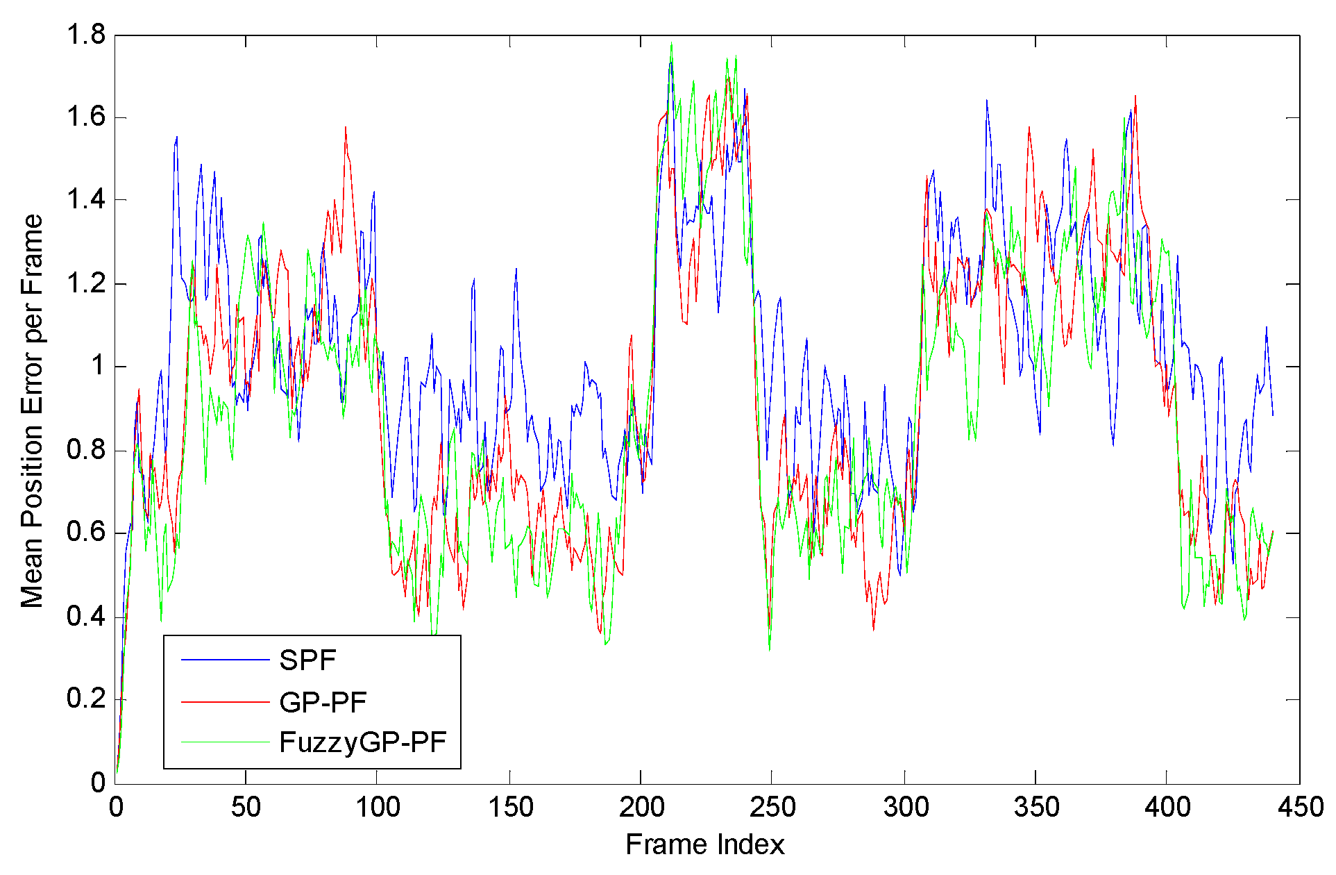
Figure 1 shows the tracking results by the SPF, the GP-PF, and the proposed FuzzyGP-PF. For a more clear view of the differences of the tracking performance by different methods, Figure 2 shows the mean error per frame of estimated position corresponding to the three methods. It is clear that when the target is during the maneuvering, the SPF cannot maintain good tracking accuracy. This happens because the target state changes dramatically, the most particles can no longer represent the true motion of the target well and, thus, the weights of these particles become negligible. Under such circumstance, the SPF cannot work well. Besides that, we can see that the speed of target changing abruptly leads to the increase of the mean position error of GP-PF and FuzzyGP-PF, but the FuzzyGP-PF work better than GP-PF, obviously.

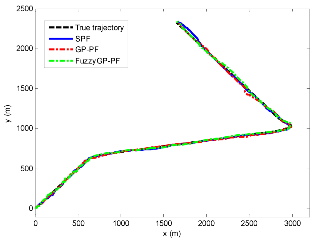
Figure 1. Estimated trajectory by the SPF, GP-PF, and FuzzyGP-PF.

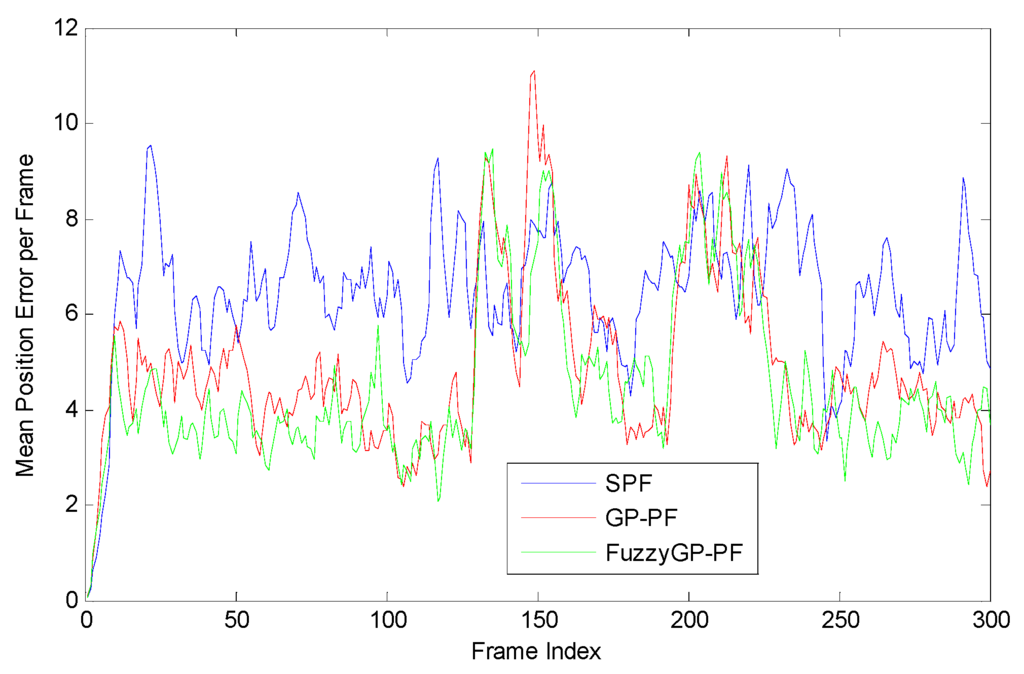
Figure 2. Mean position error per frame by SPF, GP-PF, and FuzzyGP-PF.

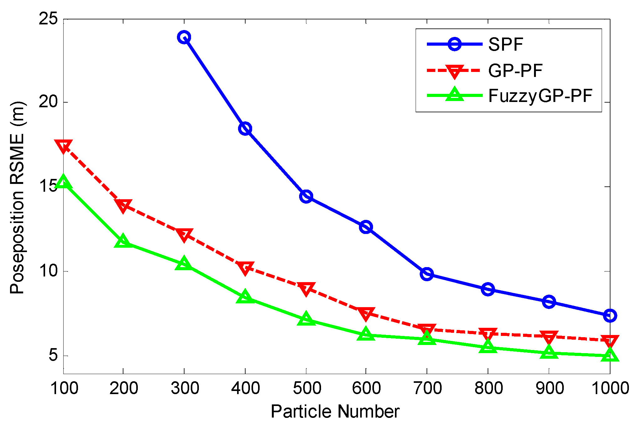
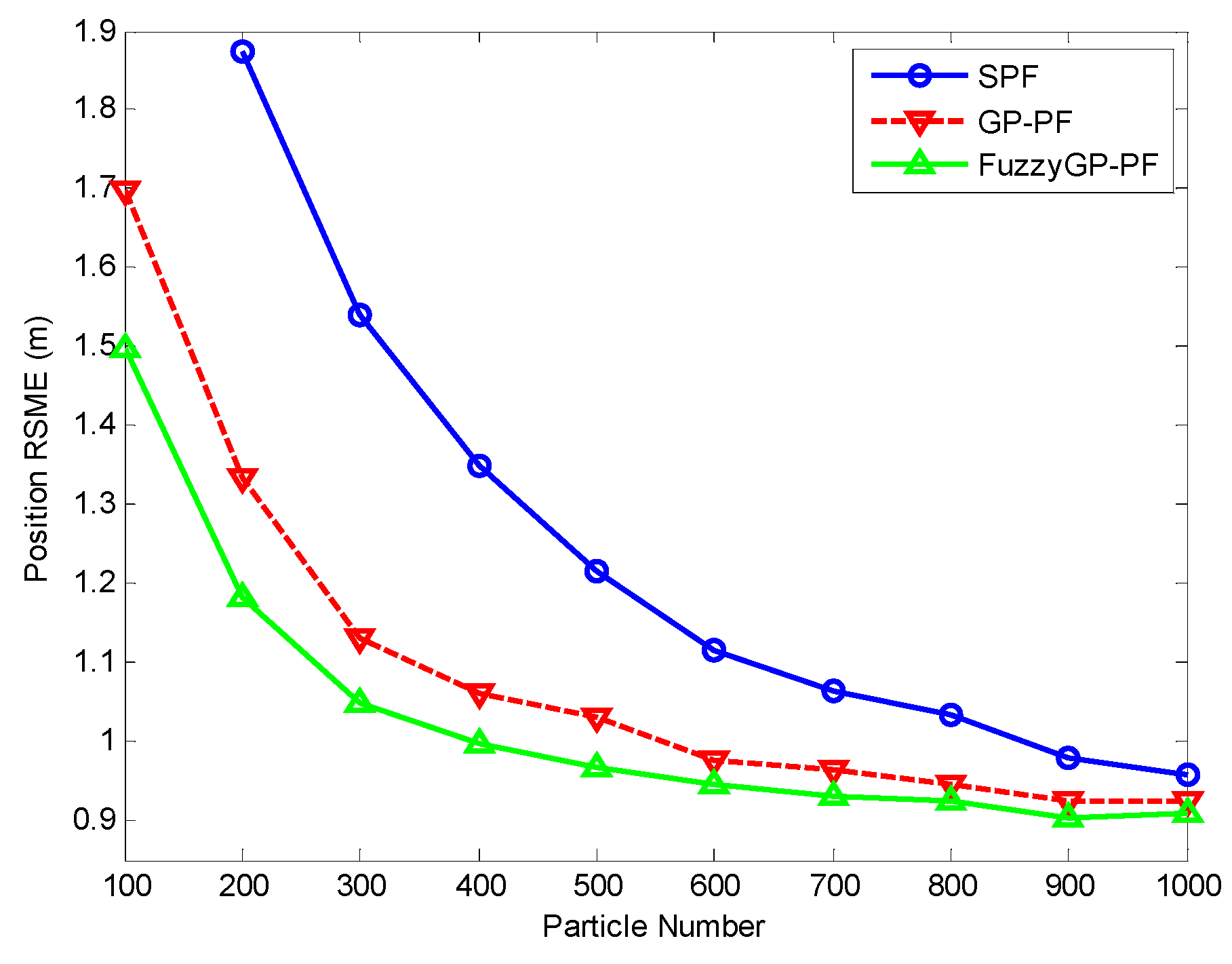
In order to analyze the tracking performance with different particle numbers by the three filters, Figure 3 shows the position RMSE in 100 dependent runs when the particle number changes from 100 to 1000. It is shown in Figure 3 that our method is better than the others. Notably, the SPF has no data because of tracking lost when particles is smaller than 300.

Figure 3. Position RMSE by SPF, GP-PF, and FuzzyGP-PF with different particle numbers.

In order to analyze the robustness of the proposed FuzzyGP-PF to Q and R variation, Figure 4 plots the position RMSE in 100 dependent runs when the Q₀ and R₀ changes from one time to 4096 (4⁶) times where Q₀ = [1, 0; 0, 1], R₀ = [1, 0; 0, 1]. As can be seen in Figure 4, the tracking accuracy of the three methods is approximately the same when Q and R are small. However, the tracking accuracy is much better than GP-PF with the increase of the Q and R. That is to say that the proposed FuzzyGP-PF algorithm can enhance the robustness of tracking when the noise of the tracking circumstances is larger. Just as in Figure 3, the SPF has no data because of tracking lost when the Q and R are 4096.

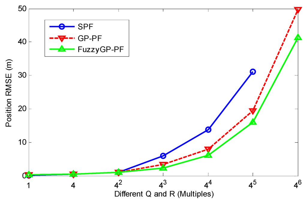
Figure 4. Position RMSE by SPF, GP-PF, and FuzzyGP-PF with different Q and R.

Table 3 gives the tracking performance of the FuzzyGP-PF with different numbers of particles used in the fuzzy grey prediction sampling, when a total of 1000 particles are used. It shows that an optimal particle number for fuzzy grey prediction can be obtained by running simulations. In actuality, a small N_grey is enough for most cases.

Table 3. Tracking performance of FuzzyGP-PF with different N_grey (total particle number: 1000).

Ngrey/N	5%	10%	20%	50%	70%	90%
Position RMSE (m)	5.8172	5.6039	5.9719	7.1727	7.4432	7.6792
Consumption Time (s)	15.1039	14.9525	15.2948	14.3329	15.4187	15.5165

4.2. Scenario 2: Large Maneuvers with Constant Turn Model

4.2.1. Motion Model

In this case, we consider a relatively complicated scenario where the motion pattern of the target changes more largely and the maneuvering speed is very slow. The target is modeled by the coordinated turn (CT) model:

$$x_k=F(\theta ,T)x_{k-1}+B{\omega }_k$$

(23)

where $F(\theta ,T)=\left(\begin{array}{cccc}1& \frac{\sin \theta T}{\theta }& 0& -\frac{1-\cos \theta T}{\theta }\\ 0& \cos \theta T& 0& -\sin \theta T\\ 0& -\frac{1-\cos \theta T}{\theta }& 1& \frac{\sin \theta T}{\theta }\\ 0& \sin \theta T& 0& \cos \theta T\end{array}\right)$ is the state transition matrix, $\theta$ is the turn rate, and the other parameters are the same as Scenario 1.

The target starts a constant velocity motion from position (100 m, 100 m) with initial speed $v_x=2.8m/s$, $v_y=2.8m/s$, and $\theta =0°/s$. Table 4 lists the detailed description of the target motion. The significant difference between the two scenarios lies in the target motion speed.

Table 4. Description of object motion.

Time Index (0.5 s)	Object Motion
0–20	Constant velocity
21–100	Constant turn (6°/s)
101–200	Constant velocity
201–240	Constant turn (9°/s)
241–300	Constant velocity
301–400	Constant turn (−7°/s)
401–440	Constant velocity

4.2.2. Tracking Performance Comparison

The common parameters in this case are given as follows: the particle number for grey prediction is N_grey = N/10, L = 10 (L is used for sampling step in fuzzy grey prediction algorithm); a = 0.01, b = 0.1, c = 0 (a, b, c is used for the fuzzy membership function); sampling interval T = 0.5 s; Q = [4, 0; 0, 4], R = [4², 0; 0, 4²] (Q and R is covariance matrix used for noise vector). The first six parameters are the same as Scenario 1, the Q and R are changed since the tracking lost probability of SPF is 100% when Q = [4², 0; 0, 4²] and R = [20², 0; 0, 20²].

Table 5 shows the tracking results by the SPF, the GP-PF, and the proposed FuzzyGP-PF when the particle number N is 500. Conclusions drawn from Table 5 are similar from the Table 2, the major difference between them is that the tracking lost probability of SPF is decreased when Q and R are significantly reduced.

Table 5. Tracking performance comparison (number of particles is 500).

Algorithms	Position RMSE (m)	Consumption Time (s)	Tracking Lost Probability (%)
SPF	1.2020	12.1559	3%
GP-PF	1.1814	12.3246	0%
FuzzyGP-PF	1.1425	12.4627	0%

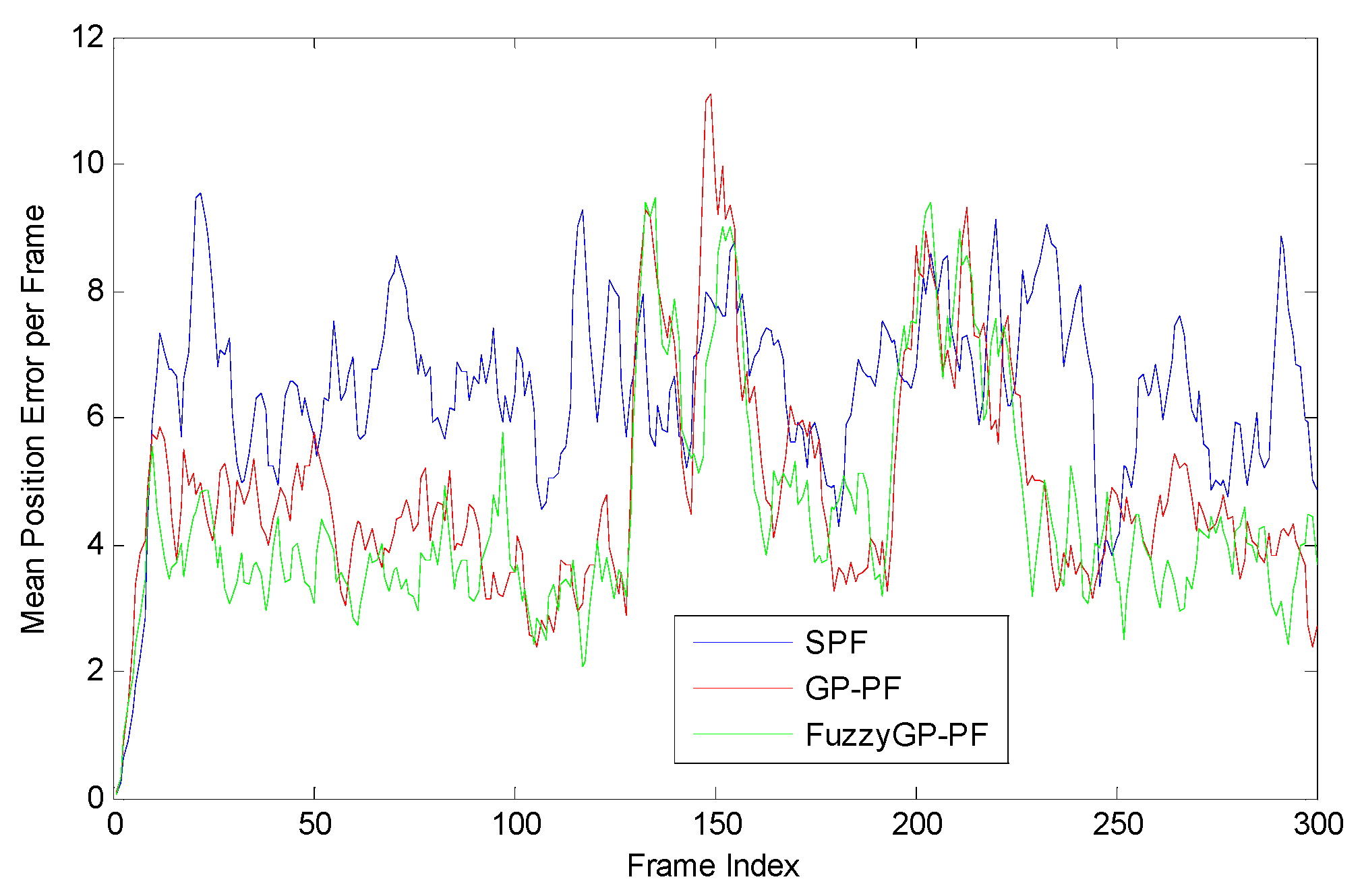
Figure 5 shows the tracking results by the SPF, the GP-PF, and the proposed FuzzyGP-PF. For a more clear view of the differences of the tracking performance by different methods, Figure 6 shows the mean error per frame of the estimated position corresponding to the three methods. We can see that the FuzzyGP-PF works better than SPF and GP-PF most of the time.

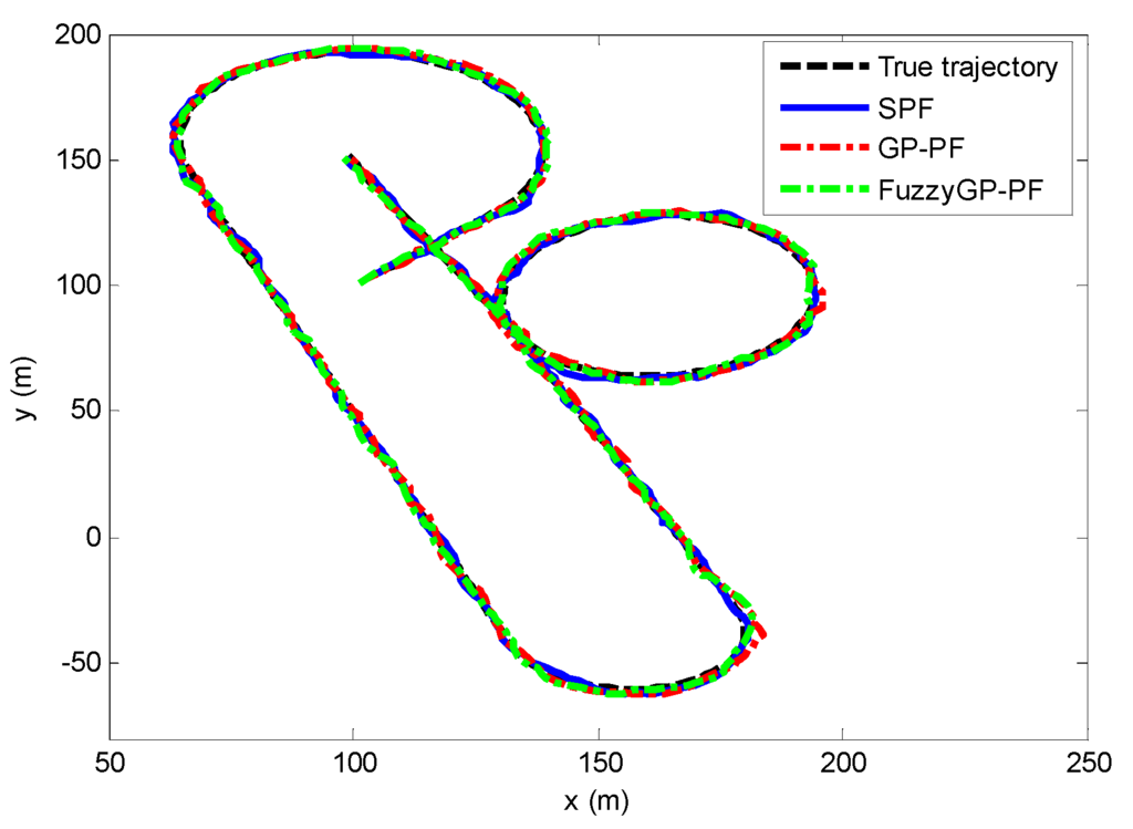
Figure 5. Estimated trajectory by the SPF, GP-PF, and FuzzyGP-PF.

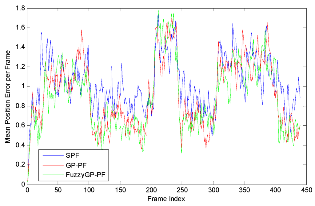
Figure 6. Mean position error per frame by SPF, GP-PF, and FuzzyGP-PF.

In order to analyze the tracking performance in Scenario 2 with different particle number by the three filters, Figure 7 shows the position RMSE in 100 dependent runs when the particle number changes from 100 to 1000. It is shown in Figure 7 that our method is better than the others. Notably, the SPF has no data because of tracking lost when particles is smaller than 100.

Figure 7. Position RMSE by SPF, GP-PF, and FuzzyGP-PF with different particle numbers.

In order to analyze the robustness of the proposed FuzzyGP-PF to Q and R variation in Scenario 2, Table 6 shows the position RMSE in 100 dependent runs when the Q₀ and R₀ changes from one time to 4096 (4⁶) times where Q₀ = [1, 0; 0, 1], R₀ = [1, 0; 0, 1]. From Table 6, the advantage of the proposed FuzzyGP-PF is more obvious. It is more effective and robust than the SPF and the GP-PF. Notably, SPF has no data because of tracking lost when the times of Q₀ and R₀ are greater than 256 (4⁴).

Table 6. Position RMSE by SPF, GP-PF, and FuzzyGP-PF with different Q and R.

Different Q and R (The Times of Q0 and R0)	1 Time	4 Times	42 Times	43 Times	44 Times	45 Times	46 Times
RMSE by SPF (m)	0.4176	0.5139	1.0740	2.9582	NaN	NaN	NaN
RMSE by GP-PF (m)	0.4122	0.5062	1.0615	2.9002	9.5648	33.2356	92.3366
RMSE by FuzzyGP-PF (m)	0.4030	0.4965	1.0371	2.8696	9.1918	31.1210	90.6894

Now we make a summary of the two cases: the two cases are very typical; in the first one, the target motion has relatively high speed and acceleration; the second one has a more complex motion pattern and very slow speed. From the above comparisons, one can conclude that the overall performance of the proposed FuzzyGP-PF is superior to the SPF and the GP-PF under various circumstances.

5. Conclusions

In this paper, we proposed an improved particle filter based on fuzzy grey prediction for object tracking. By virtue of incorporating fuzzy mathematics theory into grey prediction, a new fuzzy grey prediction model is established. The proposed particle filter algorithm combining the fuzzy grey prediction model can improve the structure of particles and, thus, it can express the posterior density more effectively. To conclude, the advantages of the proposed FuzzyGP-PF algorithm comparing with the SPF and GP-PF are mainly focused on three aspects: improving estimation accuracy significantly; overcoming the problems of tracking lost well, even when the number of particles is very small; and enhancing the robustness of tracking when the noise of the tracking circumstances is larger. In addition to this, the computational complexity is comparable with the SPF and GP-PF for obtaining the same level of accuracy. Simulation results show the above conclusion.

References

- Banerjee, A.; Burlina, P. Efficient particle filtering via sparse kernel density estimation. IEEE Trans. Image Process. 2010, 19, 2480–2490. [Google Scholar] [CrossRef] [PubMed]
- Khakpour, F.; Ardeshir, G. A novel algebraic method for kernel-based object tracking. Comput. Electr. Eng. 2014, 40, 1482–1497. [Google Scholar] [CrossRef]
- Bray, M.; Kollermeier, E.; Vangool, L. Smart particle filtering for high-dimensional tracking. Comput. Vis. Image Underst. 2007, 106, 116–129. [Google Scholar] [CrossRef]
- Singh, A.K.; Kumar, P.; Chakravarty, T.; Singh, G.; Bhooshan, S. A novel digital beam former with low angle resolution for vehicle tracking radar. Prog. Electromagn. Res. 2006, 66, 229–237. [Google Scholar] [CrossRef]
- Hong, S.H.; Shi, Z.G.; Chen, K.S. Novel roughening algorithm and hardware architecture for bearings-only tracking using particle filter. J. Electromagn. Waves Appl. 2008, 22, 411–422. [Google Scholar] [CrossRef]
- Yim, J.; Jeong, S.; Gwon, K.; Joo, J. Improvement of Kalman filters for WLAN based Indoor Tracking. Expert Syst. Appl. 2010, 37, 426–433. [Google Scholar] [CrossRef]
- Mónica, F.B.; Xu, S.; Djurić, P.M. Performance comparison of EKF and particle filtering methods for maneuvering targets. Digit. Signal Process. 2007, 17, 774–786. [Google Scholar]
- Weng, S.K.; Kuo, C.M.; Tu, S.K. Video object tracking using adaptive Kalman filter. J. Vis. Commun. Image Represent. 2006, 17, 1190–1208. [Google Scholar] [CrossRef]
- Van der Merwe, R.; Doucet, A.; de Freitas, N.; Wan, E. The Unscented Particle Filter; Cambridge University Engineering Department: Cambridge, UK, 2000. [Google Scholar]
- Wan, E.; van der Merwe, R. The Unscented Kalman Filter; Cambridge University Engineering Department: Cambridge, UK, 2000. [Google Scholar]
- Ershen, W.; Tao, P.; Zhixian, Z.; Pingping, Q. GPS receiver autonomous integrity monitoring algorithm based on improved particle filter. J. Comput. 2015, 9, 2066–2074. [Google Scholar]
- Gordon, N.J.; Salmond, D.J.; Smith, A.F.M. Novel approach to nonlinear/non-Gaussian Bayesian state estimation. IEEE Proc. F 1993, 140, 107–113. [Google Scholar] [CrossRef]
- Kong, X.; Chen, Q.; Xu, F.; Gu, G.; Ren, K.; Qian, W. Motion object tracking based on the low-rank matrix representation. Opt. Rev. 2015, 22, 786–801. [Google Scholar] [CrossRef]
- Abdelali, H.A.; Essannouni, F.; Essannouni, L.; Aboutajdine, D. A new moving object tracking method using particle filter and probability product kernel. In Proceedings of Intelligent Systems and Computer Vision (ISCV), Fez, Morocco, 25–26 March 2015.
- Arulampalam, M.S.; Maskell, S.; Gordon, N.; Clapp, T. A tutorial on particle filters for online nonlinear/non-Gaussian Bayesian tracking. IEEE Trans. Signal Process. 2002, 50, 174–188. [Google Scholar] [CrossRef]
- Pitt, M.K.; Shephard, N. Filtering via simulation: Auxiliary particle filters. J. Am. Stat. Assoc. 1999, 94, 590–599. [Google Scholar] [CrossRef]
- Smith, L.; Aitken, V. The Auxiliary Extended and Auxiliary Unscented Kalman Particle Filters. In Proceedings of the Canadian Conference on Electrical and Computer Engineering, Washington, DC, USA, 22–26 April 2007; pp. 1626–1630.
- Higuchi, T. Monte Carlo filtering using the genetic algorithm operators. J. Stat. Comput. Simul. 1997, 59, 1–23. [Google Scholar] [CrossRef]
- Orguner, U.; Gustafsson, F. Risk sensitive particle filters for mitigating sample impoverishment. IEEE Trans. Signal Process. 2008, 56, 5001–5012. [Google Scholar] [CrossRef]
- Ding, J.W.; Tang, Y.Q.; Liu, W.; Huang, Y.Z.; Huang, K.Q. Tracking by local structural manifold learning in a new SSIR particle filter. Neurocomputing 2015, 161, 277–289. [Google Scholar] [CrossRef]
- Shabat, G.; Shmueli, Y.; Bermanis, A.; Averbuch, A. Robust object tracking using semi-supervised appearance dictionary learning. Pattern Anal. Mach. Intell. 2015, 37, 1396–1407. [Google Scholar] [CrossRef] [PubMed]
- Chen, J.F.; Shi, Z.G.; Hong, S.H.; Chen, K.S. Grey prediction based particle filter for maneuvering target tracking. Prog. Electromagn. Res. 2009, 93, 237–254. [Google Scholar] [CrossRef]
- Zhu, M.Q.; Wang, Z.L.; Chen, Z.H. Visual tracking algorithm based on grey prediction model and particle filter. Control Decis. 2012, 27, 53–57. [Google Scholar]
- Kayacan, E.; Kaynak, O. Grey Prediction Based Control of a Non-Linear Liquid Level System Using PID Type Fuzzy Controller. In Proceedings of the IEEE International Conference on Mechatronics, Budapest, Hungary, 3–5 July 2006; pp. 292–296.
- Deng, J.L. Control problems of grey system. Syst. Control Lett. 1982, 5, 288–294. [Google Scholar]
- Li, X.R.; Jilkov, V.P. Survey of maneuvering target tracking—Part I: Dynamic models. IEEE Aerosp. Electron. Syst. Mag. 2003, 39, 1333–1364. [Google Scholar]
© 2016 by the authors; licensee MDPI, Basel, Switzerland. This article is an open access article distributed under the terms and conditions of the Creative Commons Attribution (CC-BY) license (http://creativecommons.org/licenses/by/4.0/).