Microfluidic Network Simulations Enable On-Demand Prediction of Control Parameters for Operating Lab-on-a-Chip-Devices

Abstract

Reliable operation of lab-on-a-chip systems depends on user-friendly, precise, and predictable fluid management tailored to particular sub-tasks of the microfluidic process protocol and their required sample fluids. Pressure-driven flow control, where the sample fluids are delivered to the chip from pressurized feed vessels, simplifies the fluid management even for multiple fluids. The achieved flow rates depend on the pressure settings, fluid properties, and pressure-throughput characteristics of the complete microfluidic system composed of the chip and the interconnecting tubing. The prediction of the required pressure settings for achieving given flow rates simplifies the control tasks and enables opportunities for automation. In our work, we utilize a fast-running, Kirchhoff-based microfluidic network simulation that solves the complete microfluidic system for in-line prediction of the required pressure settings within less than 200 ms. The appropriateness of and benefits from this approach are demonstrated as exemplary for creating multi-component laminar co-flow and the creation of droplets with variable composition. Image-based methods were combined with chemometric approaches for the readout and correlation of the created multi-component flow patterns with the predictions obtained from the solver.

1. Introduction

Microfluidics is the backbone of lab-on-a-chip devices [1]. Over the past decade, complex laboratory workflows have been implemented through on-chip technologies [2,3,4,5], ranging from the generation of chemical gradients [6,7], over microfluidic-based nanoparticle fabrication [8], their surface modification [9,10] to point-of-care diagnostics [11] and environmental analysis [12]. Thus, the performance requirements of microfluidic devices are increasing, and reliable control and prediction of flow rate and operating pressure are crucial. Especially pattern-based microfluidics [13] require mechanical designs tailored to their specific application, which require new and optimized approaches for the design [13,14,15] and control of microfluidic networks.

Microfluidic design automation (MDA) tools for modeling laminar flow [16,17] and droplet-based microfluidic systems have already been developed [18,19,20]. This new approach analyzes single-phase microfluidic devices that rely on the pressure-driven operation and multi-phase droplets in a continuous oil phase. A typical pressure-driven microfluidic system is the tree shape [17], with a uniform and identical cross-section over all channels, requiring proportionality between flow resistance and channel length [16]. Thus, the pressure change Δp, volume flow rate Q, and hydrodynamic resistance R can be related to a voltage change, current, and electrical resistance, respectively [16,17]. These resistive networks predict the flow rate within the microfluidic network (MFN) to obtain and provide precise data on the transport of fluids [21], on control parameters, and enables a complete computer-aided design [22].

Precise and effective tailoring of microfluidic devices towards specific applications requires reliable in-line prediction and operation of flow and pressure characteristics. Our work functionalizes the Kirchoff-based nodal analysis of MFN simulations for the in-line prediction of control pressures. We demonstrate the operation of microfluidic devices at user-defined flow rates utilizing the flow-focusing unit (FFU) of the Leibniz-IPHT PDG2 Droplet Generator Chip (PDG2) as a proof-of-concept and reference. The PDG2 platform can either create laminar co-flow of up to four components or droplets with variable composition in different regimes (dripping, transition, jetting) from up to three components. Recorded raw data and derived data tables are provided within the digital supplement.

Our work proposes an MFN solver (mfnSolver), which includes the control unit and on-chip designs. Based on the MFN and desired flow rates, initial operation pressures are calculated. In addition, pressure, volume changes, and flow rates for all on-chip channels are predicted through a translation to a respective resistive MFN. We present the proof-of-concept experiments for the proposed mfnSolver for pressure-driven microfluidics at specific flow rates. A chemometric image-based analysis analyzes the laminar and droplet flow characteristics. While we only present a limited application range of the solver, it can be further applied to iterative MDA optimizations.

2. Materials and Methods

2.1. Buffer and Sample Preparation

A 20 mmol/L sodium phosphate buffer (pH 8) was used in the experiments to avoid pH-dependent effects. The sample solutions were 2 mmol/L Bromophenol blue solution from Sigma-Aldrich Chemie GmbH (Steinheim, Germany), for which 13 mg of the sodium salt dye was dissolved in 10 mL buffer, and 4.9 mmol/L Orange G solution from Genaxxon bioscience GmbH (Ulm, Germany), containing 22 mg disodium salt dye in a 10 mL buffer. The dye buffers were diluted for the measurements to achieve a maximum absorbance between 0.3 and 0.7 inside the channel. The prepared sample solutions were filtered using HPLC certified CHROMAFIL^® RC-45/25 disposable syringe filter with a pore size of 0.45 µm and a filter diameter of 25 mm from MACHEREY-NAGEL GmbH & Co. KG (Düren, Germany) to avoid particle contamination.

The perfluorinated fluid composition dSurf (2% surfactant in Novec™ 7500), purchased from Fluigent (Paris, France), with a kinetic viscosity ν = 0.77 cm²/s and a density ρ = 1.614 g/cm³ was used as the continuous phase for droplet generation.

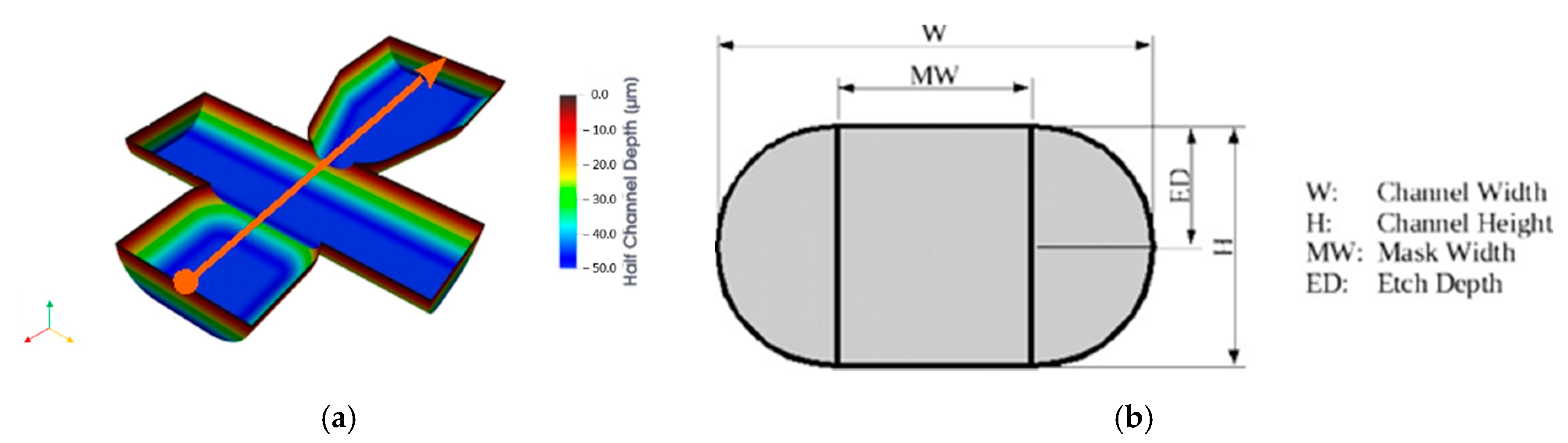
2.2. Microfluidic Chip Fabrication and Chip Preparation

The two-layer glass microfluidic chip was prepared by photolithography and wet-etching of the glass wafers (thickness 0.7 mm) with a refractive index of 1.47 with hydrofluoric acid with a uniform etching depth of 100 µm mask with a nickel-chromium metallization. Two micro-structured wafers were bonded face-to-face to create the full channels and geometries for the operating unit. The chip dimensions were 16.0 × 12.5 mm. The five fluid interconnection ports arranged in the D-sub scheme were fabricated using ultrasonic drilling. The standard channel width was 140 µm, the width before the flow-focusing unit was 165 µm, and the width of the observation chamber was 200 µm. The full channel height was 100 µm with a planar channel bottom.

For droplet generation, the wetting properties of the microchannel surfaces were adjusted by treatment with PlusOne Repel-Silane ES (a solution of Dimethyldichlorosilane (2% w/v) in Octamethylcyclotetrasiloxane) from GE Healthcare Bio-Sciences AB (Upsala, Sweden). After 10 min of incubation time, the microfluidic chip was rinsed with ethanol to remove residuals. The modification of the glass surfaces increases the hydrophobicity of the channel walls resulting in droplet formation of the aqueous phase components.

2.3. Microfluidic Control

The chip was operated by four PX-1 pressure-based flow controllers from Fluigent (Paris, France), ranging from 0 to 1000 mbar. The quality of set pressure and displayed pressure is illustrated in Figure 1a. The sample and buffer solutions were contained in 2 mL Fluiwell-4C vessels with a screw cap held by the Fluigent four Channel Sampling Rack Type 4C.

The pressure control unit was connected to the microfluidic chip network by PEEK HPLC capillaries with a length of 250 mm ± 5 mm with an outer diameter (OD) of 1/16”. The performance of the capillaries without flow sensors is shown in Figure 2a, as well as the resulting inner diameter (ID) of 0.136 mm per channel calculated based on its throughput characteristics in Figure 2b.

For control and validation of the inlet pressure settings for each channel, flow sensing units size M with an operating range of 0–80 µL/min ± 2.6 µL/min were used together with a flow sensor board from Fluigent (Paris, France). The quality of the calibrated flow sensing units carrying the buffer solution and dSurf is displayed in Figure 1b. The flow sensors were followed by another set of four PEEK HPLC capillaries with a length of 250 mm ± 5 mm, which were connected to HPLC-Teflon capillaries of length 60 mm, with an OD of 1/16” and an ID of 0.5 mm all by JASCO Deutschland GmbH (Pfungstadt, Germany) and connected through ROTILABO^® Silicone Standard sleeves of length 15 mm with an inner diameter of 1 mm from Carl Roth GmbH + Co. KG (Karlsruhe, Germany). The fluid management was controlled with the real-time software tool ALL-in-One (A-i-O) from Fluigent (Paris, France). This software allows to monitor and record the pressure status and flow rates in parallel. For the validation experiments, several measurement modes with different pressure settings were used. The graphical user interface (GUI) allows creating, editing, and loading pre-defined pressure profiles, e.g., calculated by the presented solver, for ease of use during experiments.

2.4. Optical Setup and Image Acquisition

The optical setup was a self-built microscope. A self-made LED module with a 3W 3000K LED from CREE Inc. (Durham, USA) with charcoal lighting is used as a transmission light source. The chip holder was integrated into an XY linear stage from Märzhäuser Wetzlar GmbH & Co. KG (Wetzlar, Germany). A microscopy objective from Mitutoyo Corporation (Kawasaki, Japan) with a 10× magnification, numerical aperture (NA) of 0.28, and working distance (WD) of 34 mm was used. In addition, a tube lens with a magnification of 0.5 from Opto GmbH (Gräfelfing, Germany) was used. Thus, the total magnification of the system is 5×. A color camera acA1920-155uc from Basler AG (Ahrensburg, Germany) was used to record the experiments. The validation experiments were recorded at a frame rate of 1 Hz 16-bit for 10 s per pressure profile with an exposure time of 100 µs. An additional long run of 90 s has been performed to demonstrate the stability of the flow pattern. Image processing and data analysis workflow are described in chapter 4.

For a complete measurement, the acquisition of the following reference images was mandatory: IM_SAMPLE, IM_BRIGHT, IM_DARK, IM_BLANK, and IM_FILLED. For, IM_FILLED all channels were uniformly filled with dye-containing buffer to measure the local optical path length d by the absorbance imaging approach [23]. In multi-colored flow, the image has to be acquired for all dye solutions available. The channel mask image IM_{CHANNEL_MASK} was obtained from IM_BLANK by thresholding to identify the pixels inside the channel.

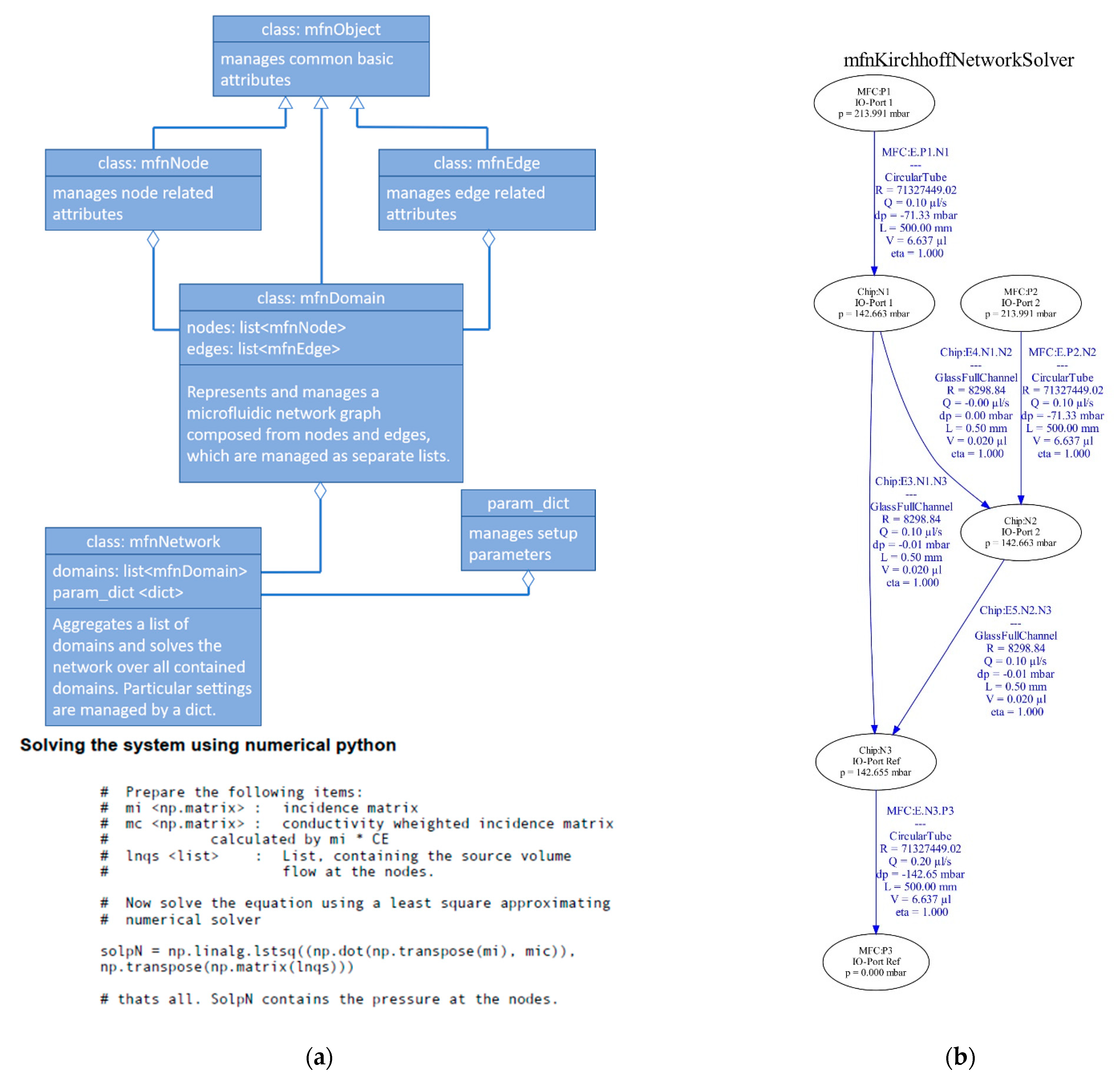
3. Microfluidic Network Solver (MfnSolver)

The presented mfnSolver is a software component for MDA. Based on Kirchhoff’s first law, that the sum of currents flowing into a junction or node equals the sum of the outflowing currents, and the second law describing the directed sum of potential differences in a closed loop is zero [24], the resulting system of linear equations of the conductors can be used to calculate the unknown potential differences or currents. In electronics, a conductor is characterized by a resistivity R as shown in Equation (1) (left), where the voltage U denominates the electrical potential difference, driving the transport of electrons through the conductor, also known as Ohm’s law. The same can be applied in fluid-dynamics, leading to the hydrodynamic resistance, as shown in Equation (1) (right),

$$\begin{array}{cc}\mathrm{R}=\frac{\mathsf{\Delta }\mathrm{U}}{\mathrm{I}},& \mathrm{R}=-\frac{\mathsf{\Delta }\mathrm{p}}{\mathrm{Q}},\end{array}$$

(1)

where the conductor is a channel, the potential unit is the pressure drop Δp, which drives the volume flow Q of volume elements through the channel, leading to the Hagen-Poiseuille equation for the hydraulic behavior [17], assuming laminar, viscous, and incompressible flow.

The presented mfnSolver overcomes the limitation of uniform cross-section. The initial network representation is a Kirchhoff-graph representation of an incidence matrix with nodes and connecting edges. Afterward, the linearized transport characteristics in terms of an edge-specific resistivity/volume/length (RVL) model are assigned to the individual edges of the network and used to create a conductivity matrix. Our work functionalizes the Kirchhoff-based nodal analysis of MFN simulations for the in-line prediction of control pressures. In particular, the user defines the flow rates along arbitrary edges of the microfluidic network, and the solver calculates the required pressure settings at the IO’s to achieve these flow rates. We demonstrate the operation of microfluidic devices at user-defined flow rates utilizing the flow-focusing unit PDG2 as a proof-of-concept and reference. Finally, the mfnSolver can be utilized to design and optimize microfluidic components, predict network performance, and automate the operation of devices based on pressure-driven fluid management schemes. The mfnSolver solves a network of representative resistive components based on Kirchhoff nodal analysis as schematically illustrated in Figure 3.

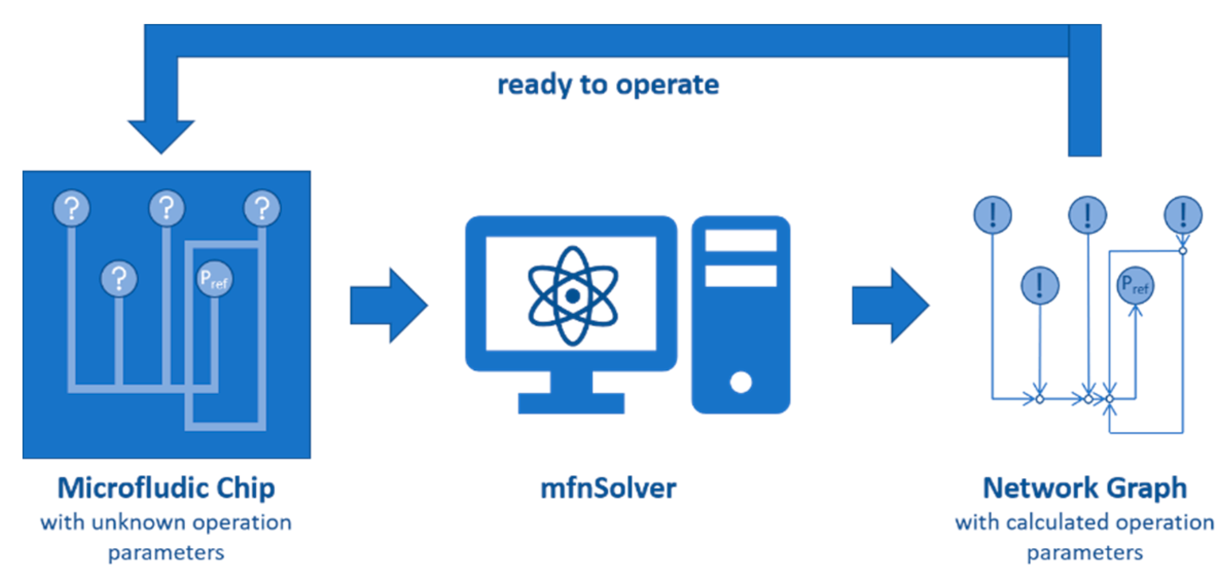
3.1. MfnSolver Concept and Implementation

The mfnSolver provides the pressure and flow rate at all defined nodes and edges. For a given network, the solution can be obtained manually or semi-automatically using computer algebra systems. However, this approach requires manual problem definition as a system of linear equations. For a single, well-defined configuration, this approach is goal-directed. However, for the iterative investigation and optimization of a large number of network configurations in dialogue with the future user, this approach is inefficient.

Kirchhoff’s first law is adapted from the conservation of charge to conserving volume in microfluidic networks. The total sum of all in- and outflowing volumes equals zero at each defined node of a microfluidic network. A node has no volume on its own. Thus, each change of geometric component leading to a change in volumes, such as junction and cross-section changes, is represented by the edge connecting the nodes. Kirchhoff’s second energy conservation law is related to the balance of the hydrodynamic potential differences (pressure) around any closed network.

For a simplified demonstration, the exemplary network in Figure 4a is considered. The network consists of the nodes N1, N2, and N3 connected by the edges E3, E4, and E5. E1, E2, and E6 are linked to the microfluidic control (MFC) units via pressure-controlled Input-Output (IO) ports IO1, IO2, and IO_ref, in Figure 4b. Depending on the pressure settings, they either serve es inlets or outlets. The network consisting of six nodes and six edges is translated into the system of linear equations, resulting in a binary incidence matrix with six columns and six rows. The columns represent the nodes and ports. The rows refer to the edges. The edge directed away from the node is assigned +1 and the arriving edge is assigned −1. The weights of the respective edges correspond to the inverse of the hydrodynamic resistance R.

The pressure results from Kirchhoff’s modified second low describing the volume flow through edges with

$${\mathrm{Q}}_{\mathrm{E}}=\left(\mathrm{MI}\cdot \mathrm{C}\right)\cdot {\mathrm{p}}_{\mathrm{N}}$$

(2)

where ${\mathrm{Q}}_{\mathrm{E}}$ denominates the flow rate vector, $\mathrm{MI}$ the incidence matrix, $\mathrm{C}$ the conductivity vector and ${\mathrm{p}}_{\mathrm{N}}$ is the vector providing the pressure at the nodes N. Thus, ${\mathrm{MI}}^{\mathrm{T}}\cdot \mathrm{Q}={\mathrm{Q}}_{\mathrm{Source}}$ follows for the conservation of volume, and ${\mathrm{MI}}^{\mathrm{T}}\cdot \left(\mathrm{MI}\cdot \mathrm{C}\right)\cdot {\mathrm{p}}_{\mathrm{N}}={\mathrm{Q}}_{\mathrm{Source}}$ as the matrix expression for solving p_N.

The edges and nodes of the introduced network and their chosen RVL model are implemented into the solver analog to Figure 4b. In the interest of the numerical stability of the solver, a rescaling of the base units is performed to avoid decimal numbers with high exponents. The unit length is defined as 1 mm within the system, the unit mass relates to 1 mg, and the unit time is 1 s. As a result, the parameters and respective units in

Table 1. Scaling of solver internal standard units for parameter study. The pressure output is converted to mbar.

Symbol	Description	Unit
L	Length	mm
V	volume	µL
p	pressure	mPa
Δp	pressure difference	mPa
R	hydrodynamic resistance	mPa s/µL
Q	volume flow rate	µL/s

follow the network diagram.

Specific models to represent the channel geometry of the on-chip network and the respective tubing of the MFC unit are implemented. The on-chip hydrodynamic resistance R is calculated based on the Hagen–Poiseuille law

$$\mathrm{R}=\frac{128.0\cdot \mathsf{\eta }\cdot \mathrm{L}}{\mathsf{\pi }\cdot {\mathrm{d}}_{\mathrm{H}}^4}$$

(3)

where L is the length of the respective edge and d_H is the hydraulic diameter with

$${\mathrm{d}}_{\mathrm{H}}=4\cdot \frac{\mathrm{A}}{\mathrm{P}}$$

(4)

with the area of the cross-section $\mathrm{A}=\mathrm{WM}\cdot \mathrm{ED}+0.5\cdot \mathsf{\pi }\cdot {\left(\mathrm{ED}\right)}^2$ and the perimeter $\mathrm{P}=2.0\cdot \left(\mathrm{WM}+\mathrm{ED}\right)+\mathsf{\pi }\cdot \mathrm{ED}$. Consequently, volume is defined as $\mathrm{V}=\mathrm{A}\cdot \mathrm{L}$. For the standard tubing, which connects the chip network with MFC, the calculation of the area is adjusted to represent a circular cross-section with $\mathrm{A}=\frac{\mathsf{\pi }}{4}\cdot {\mathrm{ID}}^2$ and ID as the inner diameter of the tubing.

The mfnSolver is implemented using Python with the numerical library Numpy for the matrix operations and the toolkit Graphviz for visualization and result presentation. The mfnSolver is consistently implemented object-oriented with the class hierarchy shown in Figure 5a. The class mfnObject manages essential attributes and provides them to the derived classes mfnNode (nodes of the network) and mfnEdge (edges of the network). The class mfnDomain manages subgraphs of a fluidic network consisting of nodes and edges, which can be assumed as sub-domains of the complete network, e.g., microfluidic chips with different configurations or higher-level control networks, are derived. The class mfnNetwork forms the core of the solver. It aggregates an arbitrary number of mfnDomain objects into a microfluidic network, creates and solves the Kirchhoff-matrix for the implemented system, and generates the network diagrams in .pdf and output lists in .csv format. Particular microfluidic circuits and subdomains can be implemented as reusable mfnDomain objects common in microelectronics for circuit design and simulation.

Thus, the solution shown in Figure 5b considers the microfluidic chip geometry as well as the microfluidic control units. The pressure and flow rate at all defined nodes and edges of the network are provided and can be used as initial operating conditions in pressure-driven experiments. The solution of the solver is obtained in less than 200 ms, even for more complex networks.

In the presented generic mfnSolver, based on the Kirchhoff nodal analysis, each edge on the MFN can be individually configured by choosing the appropriate RVL model. Therefore, the solver provides a set of pre-implemented RVL models representing the pressure-throughput characteristics of standard channel shapes such as a circular tube, capillary slit, rectangular channel, ellipsoidal channel, and half-ellipsoidal channel implementation, and hydraulic diameter-based approximation for channels with an arbitrary cross-sectional shape.

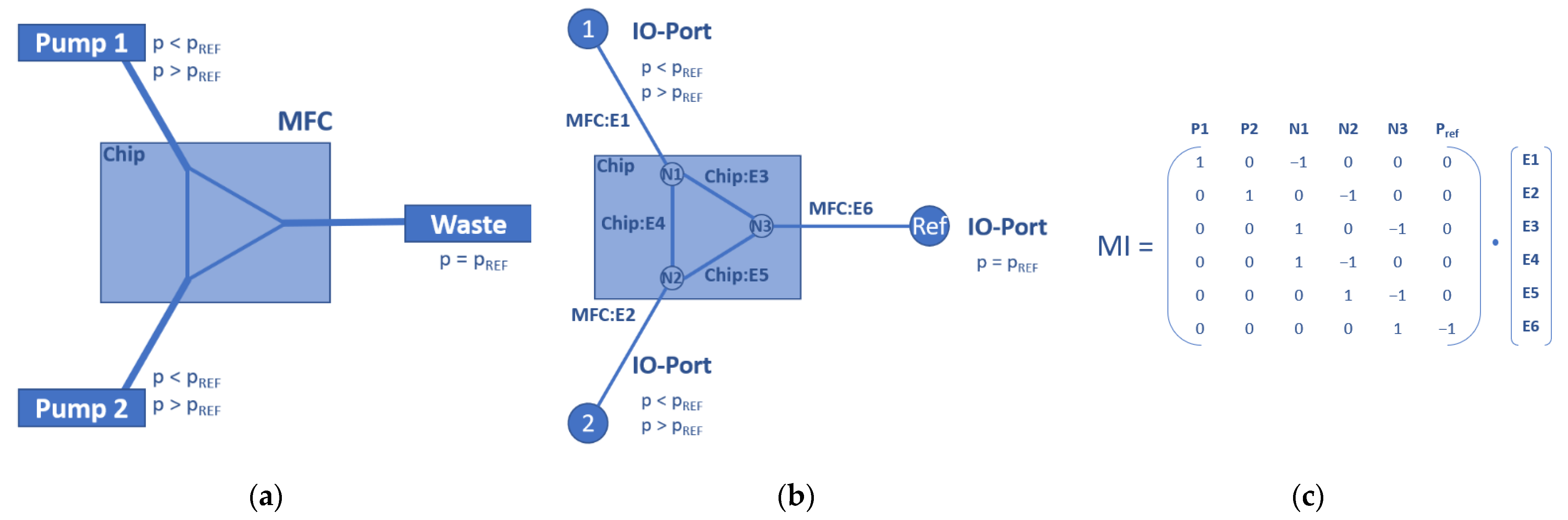
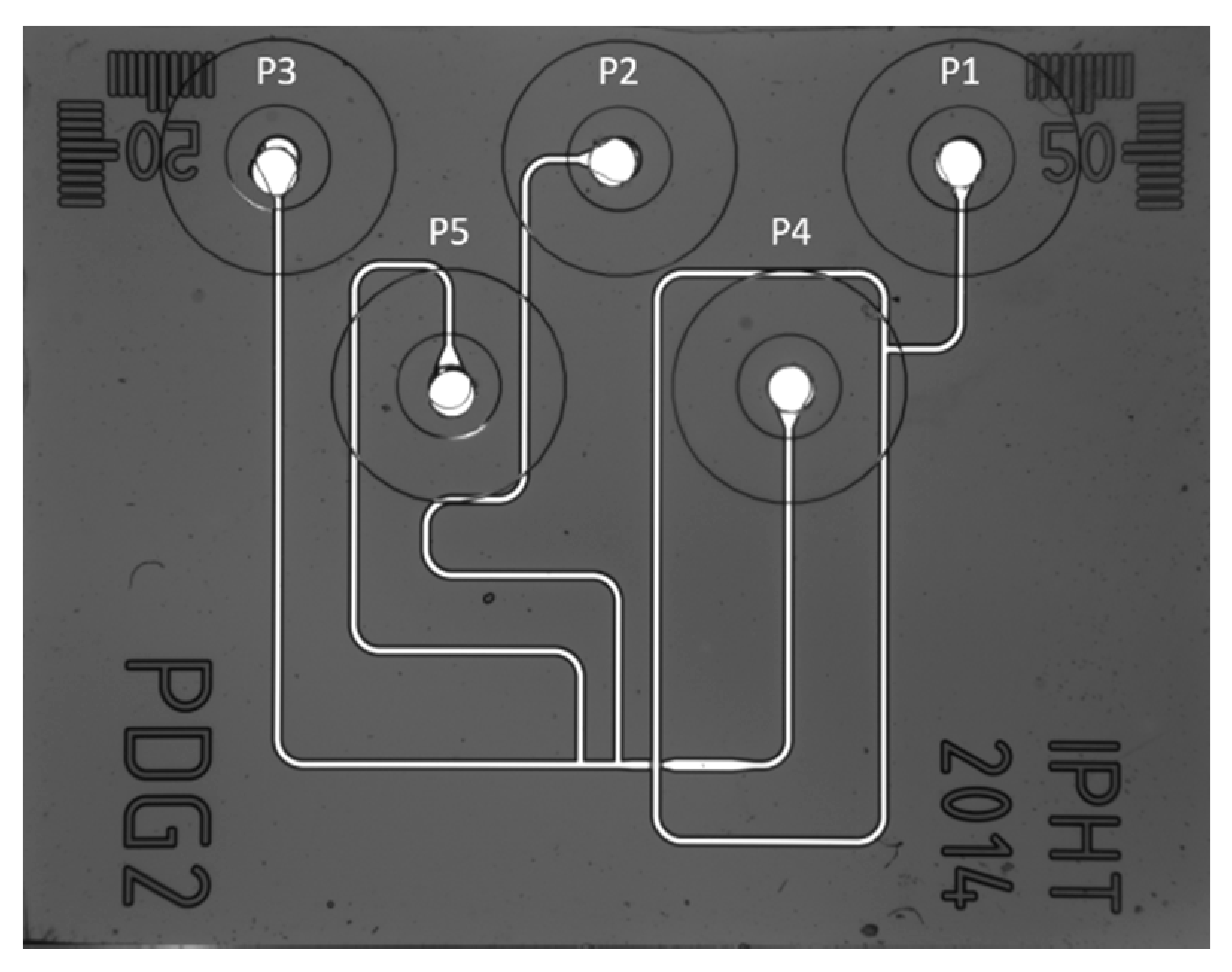
3.2. PDG2 Chip and Network Model

As an example and reference case, the mfnSolver predicts the settings for pressure-driven flow control for single and multi-phase flow utilizing the flow-focusing unit of the PDG2 chip, in Figure 6. The PDG2 on-chip MFN consists of five ports, of which four are utilized as inlets, and one is used as an outlet to waste. The three inlets P2, P3, and P5 are combined in sequence to create a multi-phase laminar flow when operated at low velocities below the turbulence threshold with Reynolds Numbers Re < π². In fluid dynamics, laminar flow is characterized by a parabular shape of the velocity gradient over the cross-section orthogonal to flow direction. This laminar dispersed phase is focused through the two-arm flow-focusing unit of inlet P1 by a continuous phase. Our PDG2 chip can be utilized for diffusion and reaction experiments at operation based on laminar co-flow.

Depending on the viscosity of the liquids and the surface functionalization of the channels, the FFU in Figure 7a can create laminar co-flows of up to four components or droplets with variable internal composition from up to three sample fluids.

The generic mfnSolver is applied to this chip geometry for MFN analysis and calculation of initial experimental pressure parameters for set flow rates to guarantee steady operation. Based on the fabrication parameter mask width WM and etch depth ED, shown in Figure 7b, the hydrodynamic resistance is calculated based on the respective cross-sectional area. The Kirchhoff-graph of the network for laminar co-flow embedded in the MFC, consisting of operation pumps, capillaries, and flow sensing units tubing to connect the control unit with the on-chip PDG2 network, is computed with the mfnSolver. The pumps 1, 2, 3, and 4 of the MFC are connected to the ports P1, P2, P3, and P5, respectively, from left to right. The outlet port P4, connected to the waste, serves as a reference with pressure p = 0 mbar. The solver uses the standard flow rate Q = 0.16 µL/s. While the flow rate of one port is gradually increased according to

Table 2. Exemplary simulation for laminar co-flow containing five flow and pressure profiles. The model flow rate as the initial solver input is opposed to the predicted pressure for each setting. The full parameter set is provided in Table S1.

		Model Flow Rate [µL/s]				Predicted Pressure [mbar]
Set	ID 1	P1	P2	P3	P5	P1	P2	P3	P5
1	1	0.08	0.16	0.16	0.16	50.568	98.783	98.925	98.797
1	2	0.16	0.16	0.16	0.16	98.980	99.142	99.284	99.156
1	3	0.32	0.16	0.16	0.16	195.806	99.860	100.003	99.874
1	4	0.64	0.16	0.16	0.16	389.457	101.297	101.439	101.311
1	5	1.28	0.16	0.16	0.16	776.759	104.170	104.312	104.184

¹ Acquisition Parameter Set Identifier (ID).

, the remaining ports are kept at a standard flow rate. In total, four different sets are modeled to predict the respective pressure outcomes analog to Table 2. The respective mfnSolver output prediction for the feedlines of an operation according to acquisition parameter ID 1 is exemplary shown in the condensed scheme in Figure 8 (top) and in more detail in Figure S1 in the digital supplement. In between the sets, the port with the varying flow rate is changed. The solver provides the predicted pressure, which is used as the input for pressure-driven operation during the experimental validation.

The Kirchhoff-graph allows tracking of the pressure drop between the nodes over the entire network. In addition, all connecting edges provide information on the selected RVL model, including their parameters, the pressure drop, the set flow rate, and the implemented dynamic viscosity η of the liquid the channel carries. The dynamic viscosity is the governing parameter that has to be adjusted to adapt the model for multi-component droplet generation. For the laminar co-flow scenario, the dynamic viscosity is assumed to match the water in all channels. This assumption also holds during the droplet experiments for the feedlines connected to P2, P3, and P5. P1 is operated with perfluorinated oil with η = ν ∙ ρ = 0.77 cm²/s ∙ 1.614 g/cm³ = 1.24278 g/(cm∙s). After the FFU, the fluid is a mixture of the oil phase and the droplets. The viscosity of this two-phase flow has been derived from the experiments by analyzing the pressure drop between the FFU as the droplet generating structure and the outlet for the utilized fixed flow rate of the formed droplet suspension. Here, a combined measured flowrate of 320 µl/s from the inlets P2, P3 and P5 was achieved by a pressure offset of 80 mbar. A shortened example of the mfnSolver prediction for the feedline pressure settings and the FFU, to create droplet flow, can be seen in Figure 8 (bottom).

To validate the presented solver, flow sensors are integrated into the feedlines to monitor the flow rate during pressure-driven operation and compare the solver results with flow measurements. In addition, the on-chip in-line flow at three different positions is measured using an RGB chemometric image-based analysis to validate the solver and compared with the respective analytical predictions of the solver. Both are discussed in the next section.

4. Experimental Validation

Within this section, the experimental validation of the introduced mfnSolver is discussed. First, flow sensors were integrated into the interconnecting capillaries. The correlation between predicted target flow rates and the experimental observation for the delivery of the fluids from the pressurized feed vessels to the Inlet-Outlet (IO)-ports of the microfluidic chip device were analyzed.

Secondly, as the experimental design does not simply integrate flow sensors into existing microfluidic devices, we switched to an optical detection method that allows measurements at arbitrary positions of the optically transparent microfluidic device. The flow-focusing chip PDG2, as introduced in the previous section, is utilized for these experiments. We generate laminar co-flows of dyed sample fluids inside the channels and perform a colorimetric analysis along profile lines orthogonal to the channel axis for the measurements. The composition of the dyed sample fluids has been varied according to the parameter profiles in Figure 9 (top) and their respective output composition (middle) and their outcome field of view (FOV) for experimental validation with the exemplary pressure profile of parameter set identifier (ID) 1 (bottom). A selection of the recorded image data for the calculated pressure settings of laminar co-flow and droplet flow is presented in Video S1, S2 and S3

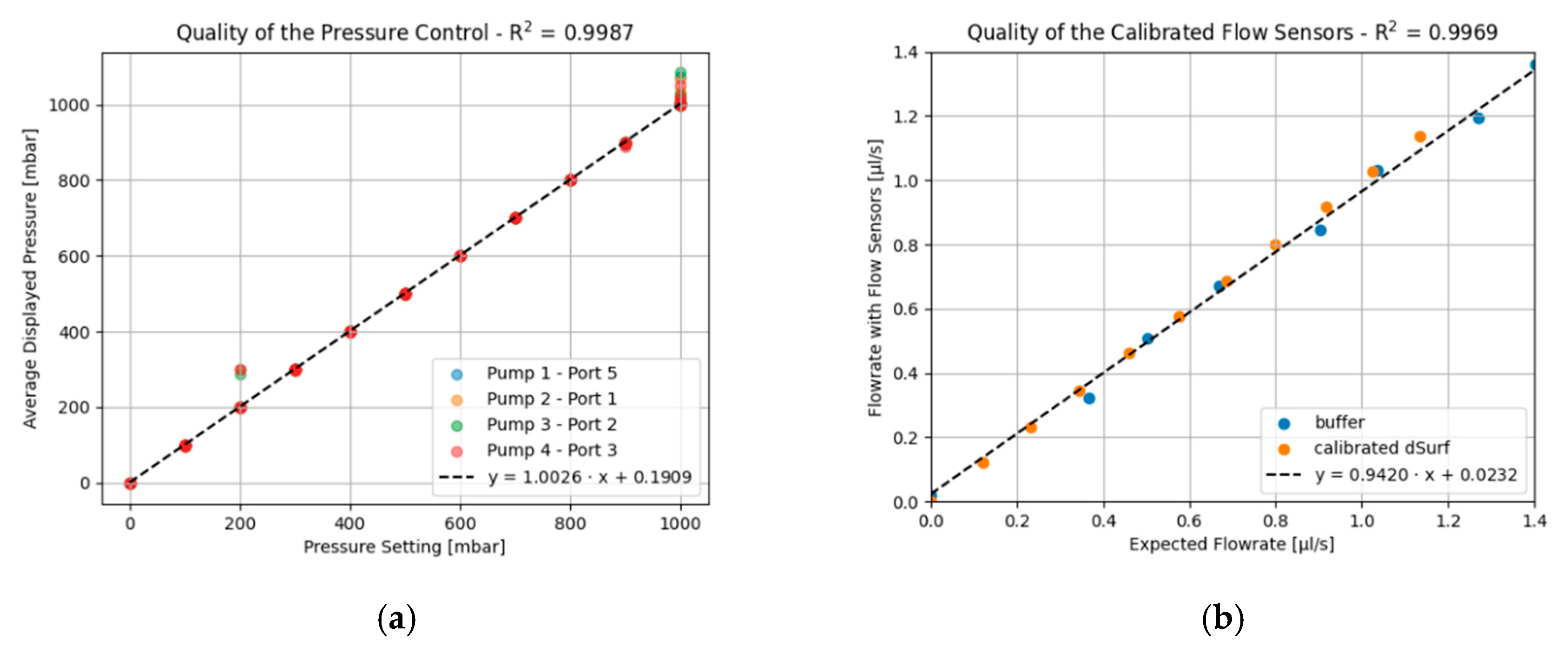
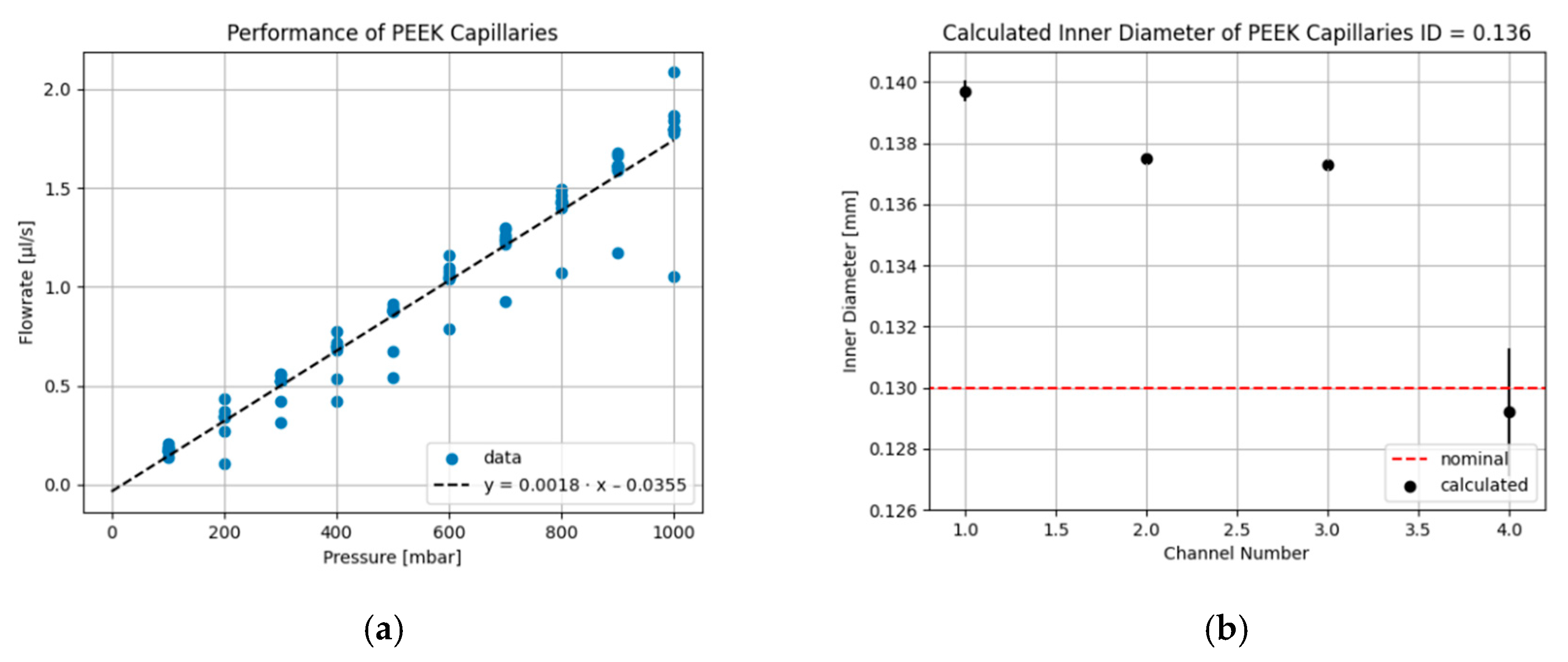
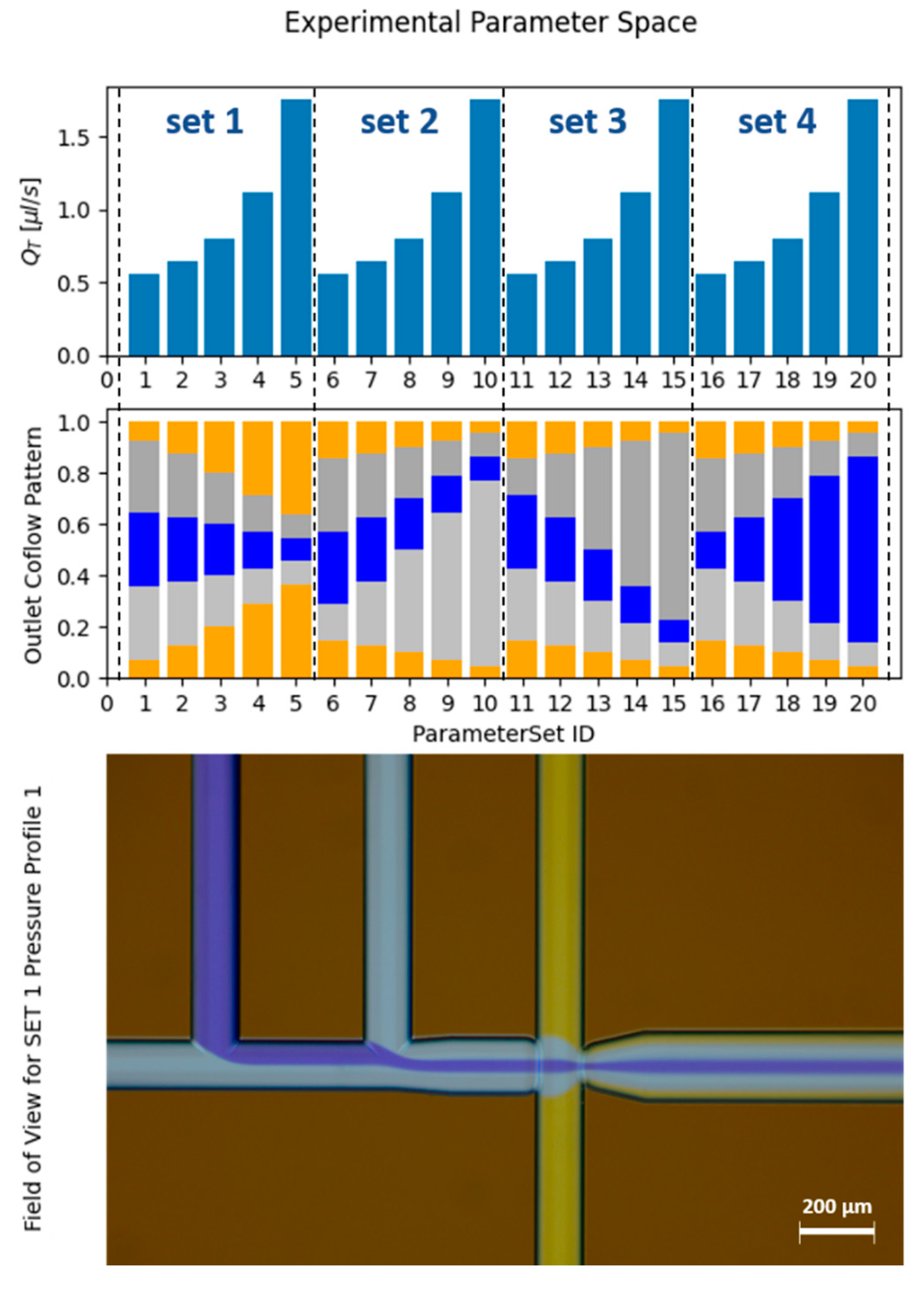
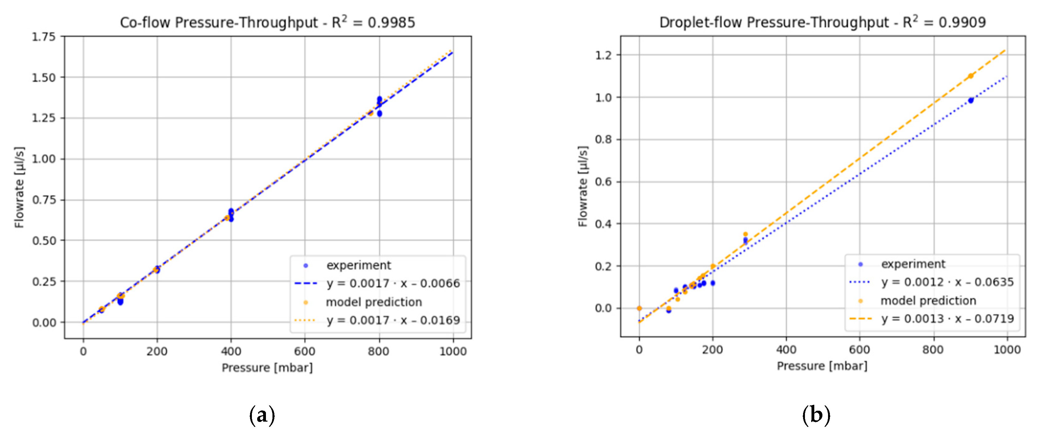
4.1. Validation of Flow Rate Prediction at Feedlines

The flow sensors are integrated into the feedline between the PEEK capillaries to monitor the flow rate during the experiment. Their performance characteristics without chip operation can be found in the Supplementary Information. A standard flow rate of 0.16 µL/s has been chosen for the model. Within each set, the flow rate through one channel is changed in five steps from 0.08 µL/s to 1.28 µL/s, while the remaining ones are set constant to the chosen standard flow rate as input for the model. The respective predicted pressure settings have been implemented as operation pressures for the PDG2 chip. The pressure is gradually increased from 50 mbar to 800 mbar, as predicted in Table 2. Each pressure setting is kept constant for 10 s. A recording of 90 s per pressure setting is performed to demonstrate flow stability of the laminar co-flow. The pressure of a port is increased from 50 mbar to 800 mbar, according to the mfnSolver calculations for laminar co-flow, which illustrates the starting and end condition of the laminar co-flow series for each set. The flow pattern was steady during all experiments, required for image-based analysis and a correlation between the phase and flow fractions.

The performance of pressure control and flow sensors is illustrated in the subsection ‘Microfluidic control’ in the chapter ‘Materials and Methods’. The comparison of the pressure-throughput characteristics predicted for laminar co-flow and the experimental parameters of the pressure control and the feedline flow sensors are shown in Figure 10a. We can conclude that the presented model based on the Kirchhoff nodal analysis can predict the overall pressure-throughput of the laminar co-flow scenario. Thus, it can be used to provide pressure-driven flow-control in the feedlines to the microfluidic chip.

For droplet generation, a laminar co-flow pattern of the three sample fluids is created as the dispersed phase. The flow-focusing unit is now functionalized as a droplet generator. The total flow rate of the dispersed phase and the continuous phase is kept constant, while the color pattern of the laminar co-flow is varied, as illustrated in Figure 11. Here, we consider evenly shaped droplets fully embedded and carried by the continuous phase. The comparison of the pressure-throughput characteristics predicted for droplet-flow and the experimental parameters are shown in Figure 10b.

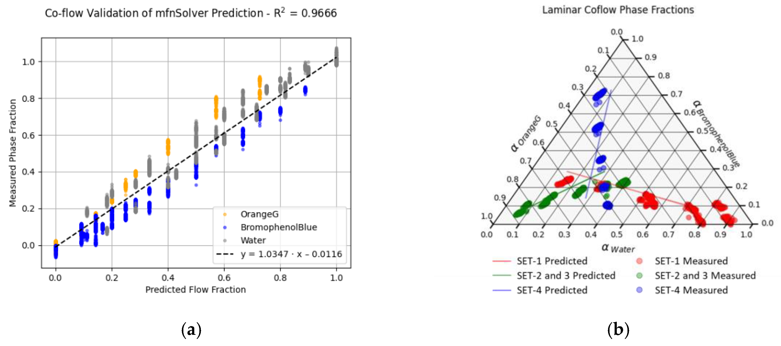
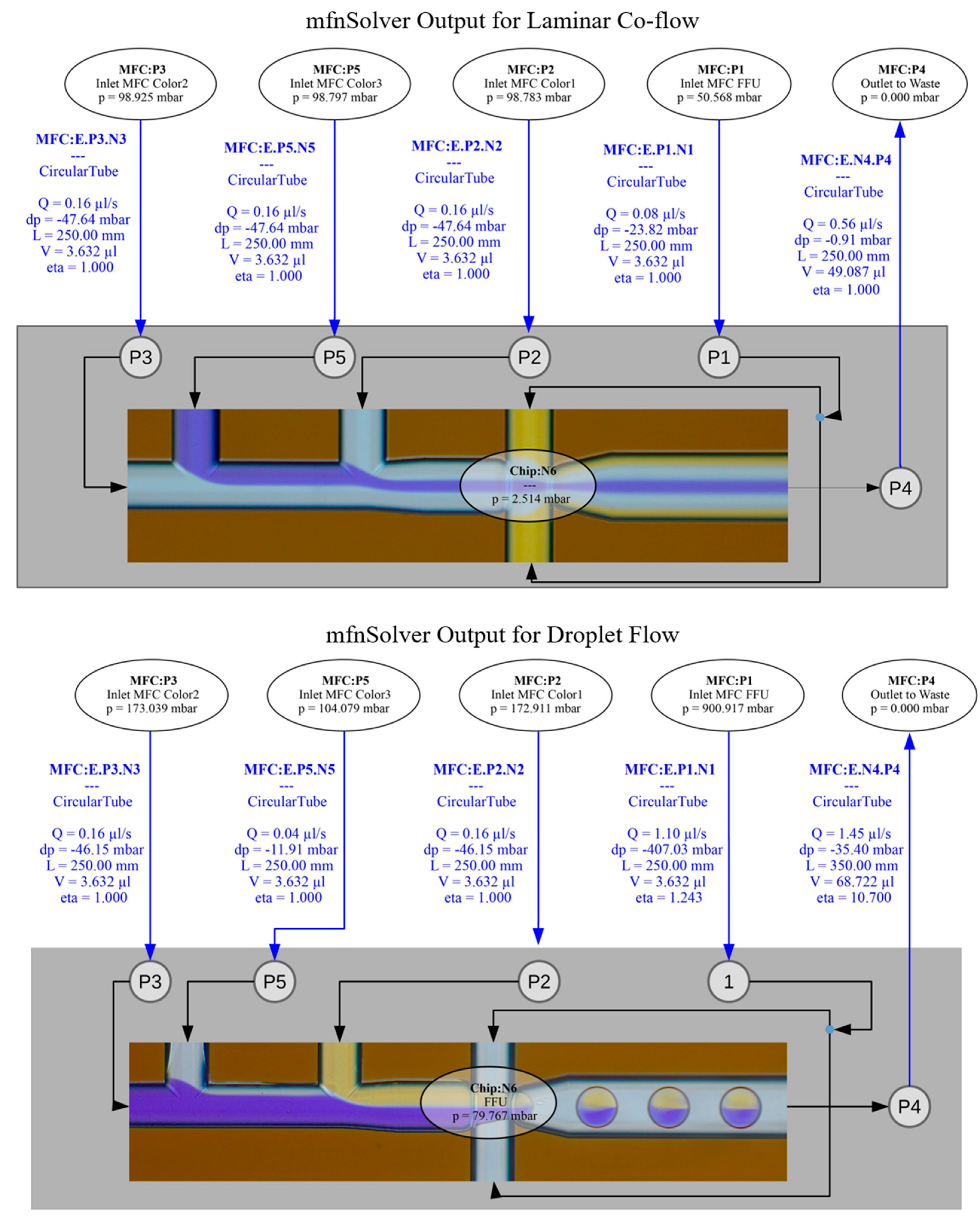
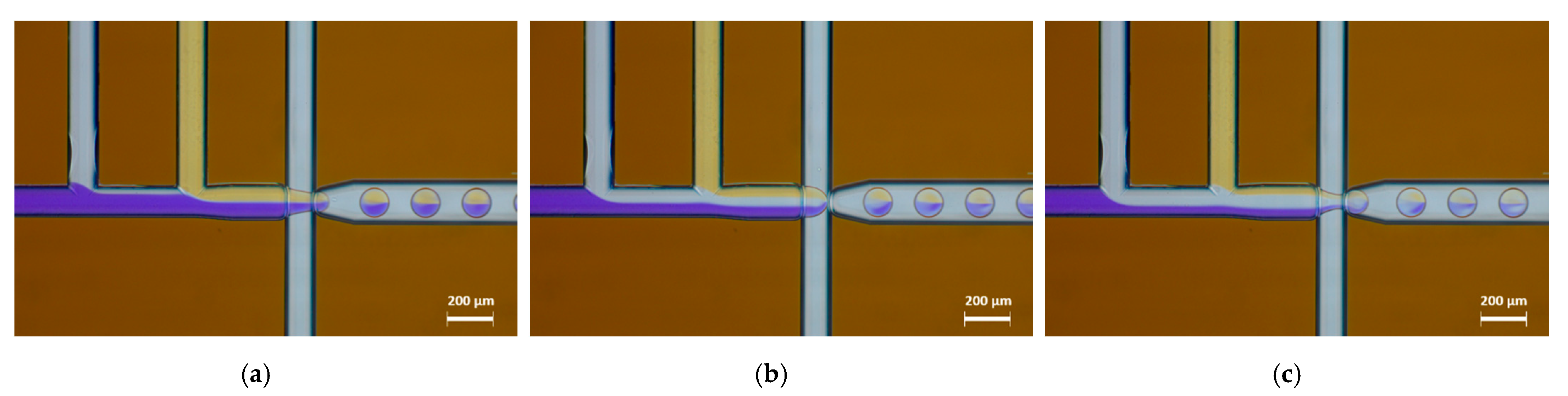
4.2. Validation of Chip Internal Flow

The majority of microfluidic devices are operated at low Reynolds Numbers with $\mathrm{Re}<{\mathsf{\pi }}^2$ as confirmed by W. Wuest [26] for channels with integrated apertures. Therefore, the formation of secondary flow patterns due to inertial forces like vortices, jets, local backflow zones, Dean-Flow patterns, or time-periodic fluctuations (e.g., Karman Vortex Street) can be neglected. The laminar flow regime allows the creation of a laminar co-flow of multiple fluid components, where each fluid component passes through the channel as a separated lamella. Diffusion is responsible for outbalancing the concentrations of the ingredients. This process is comparably slow and leads to a widening of the individual lamella and finally to a complete outbalancing of the concentration of the ingredients over time. An example for the generation of a three-component laminar co-flow in the flow-focusing chip PDG2 with the fluid components Bromophenol blue (‘BPB’), Orange G (‘OG’), and the water buffer (‘W’) is demonstrated in Figure 9. Here, the on-chip feedlines come from the top and bottom and feed into the observation channel, flowing from left to right.

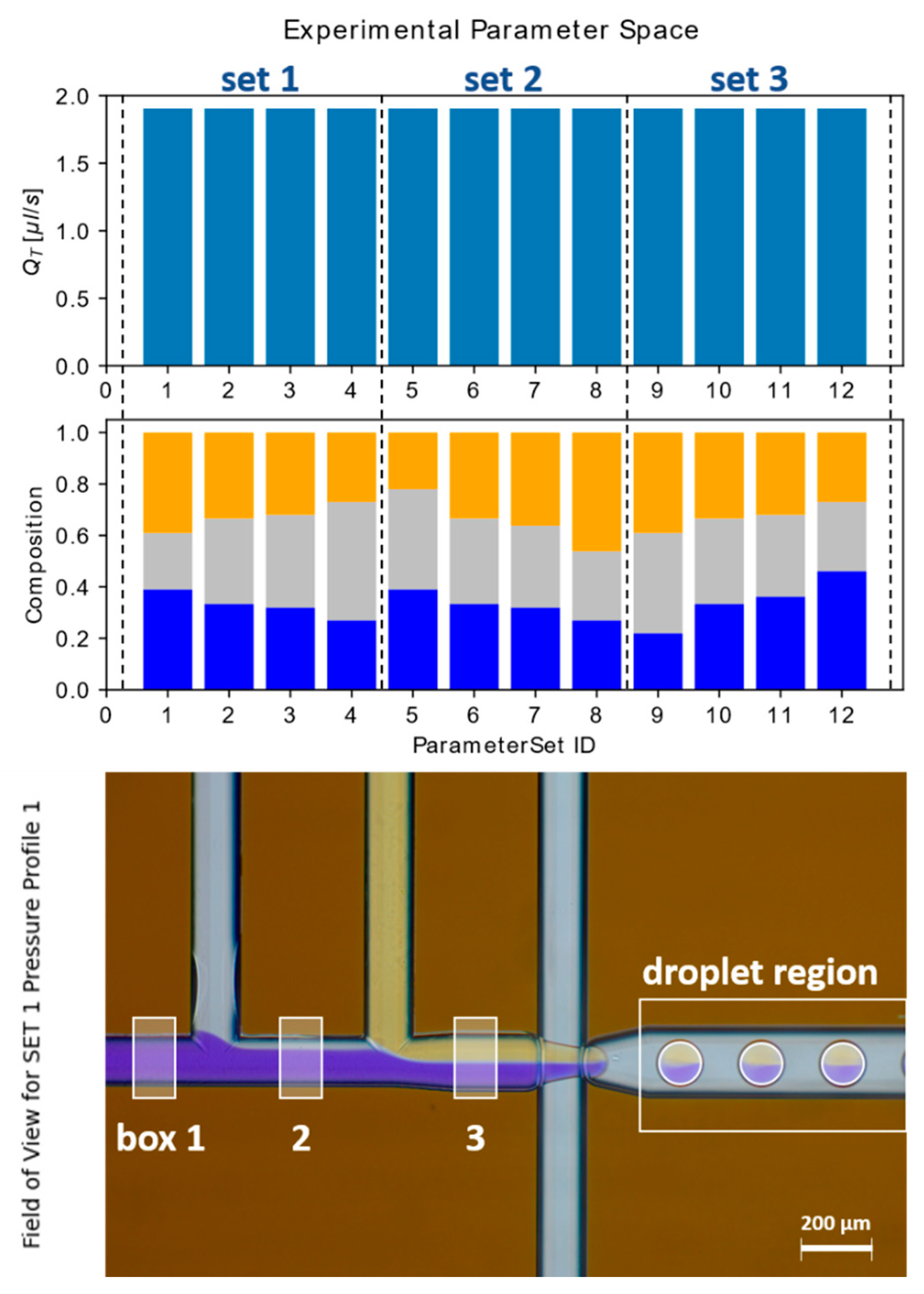
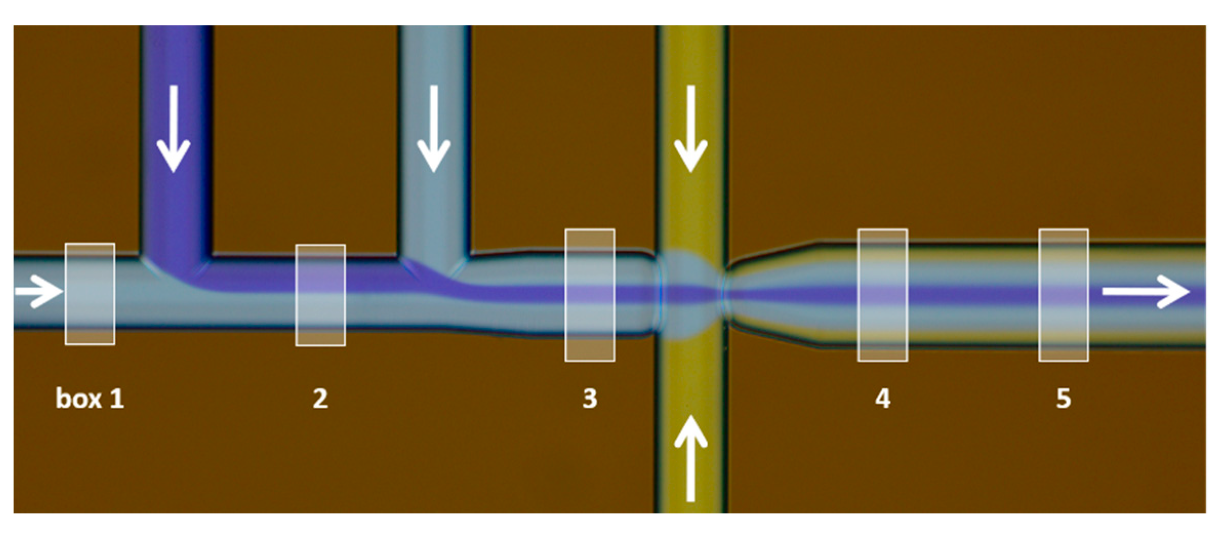
4.2.1. Data acquisition and Required Datasets

Image data are recorded by transmission mode microscopy utilizing a white light source with a condenser, a microscopy objective, and an RGB camera. Details are given in the ‘Materials and Methods’ section. Each pixel of the RGB camera acts as a three-channel photon counting device where the delivered intensity values linearly scale with the number of inclining photons. The camera is applied to measure concentrations. The raw intensities must be converted to a measured quantity, which linearly scales with the concentration c of a light-absorbing dye. According to the Beer–Lambert Law, the absorbance values A as established in UV-VIS spectroscopy and photometry conform with these requirements. Additionally, the transmitted optical path length d must be taken into account

$$\mathrm{A} =-{\log }_{10}\frac{\mathrm{I}}{{\mathrm{I}}_0}=ϵ\mathrm{cd}$$

(5)

For the conversion of the received image data to absorbance data, the following equation can be derived from Equation (5)

$${\mathrm{A}}_{\mathrm{RGB}}=-{\log }_{10} \left( \frac{{\mathrm{IM}}_{\mathrm{SAMPLE}}-{\mathrm{IM}}_{\mathrm{DARK}}}{{\mathrm{IM}}_{\mathrm{BLANK}}-{\mathrm{IM}}_{\mathrm{DARK}}} \right),$$

(6)

where IM_SAMPLE denominates the recorded image of the chip during an experimental run, IM_DARK is the recorded image with the light source switched off as the dark reference, and IM_BLANK is the recorded image of the chip for all channels filled with the buffer solution. Care must be taken in the implementation to avoid exceptions due to division by zero and logarithm of zero values. Our implementation manages these cases by substituting values below the limit of detection (LOD) in the numerator and denominator of Equation (6) by the LOD value, calculated as two times pixel noise standard deviation as measured in the acquired IM_BRIGHT, which is captured from the pure light source without the chip.

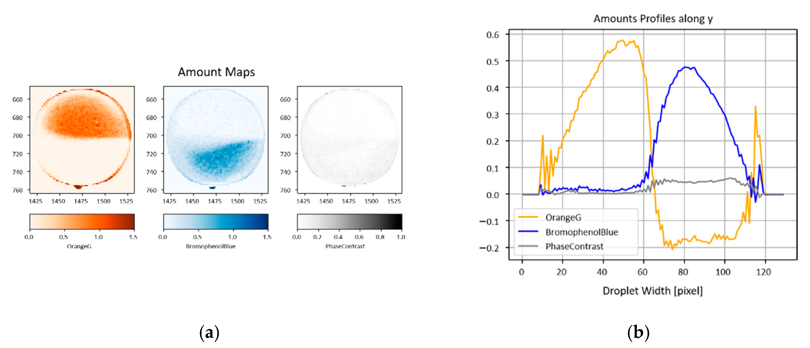
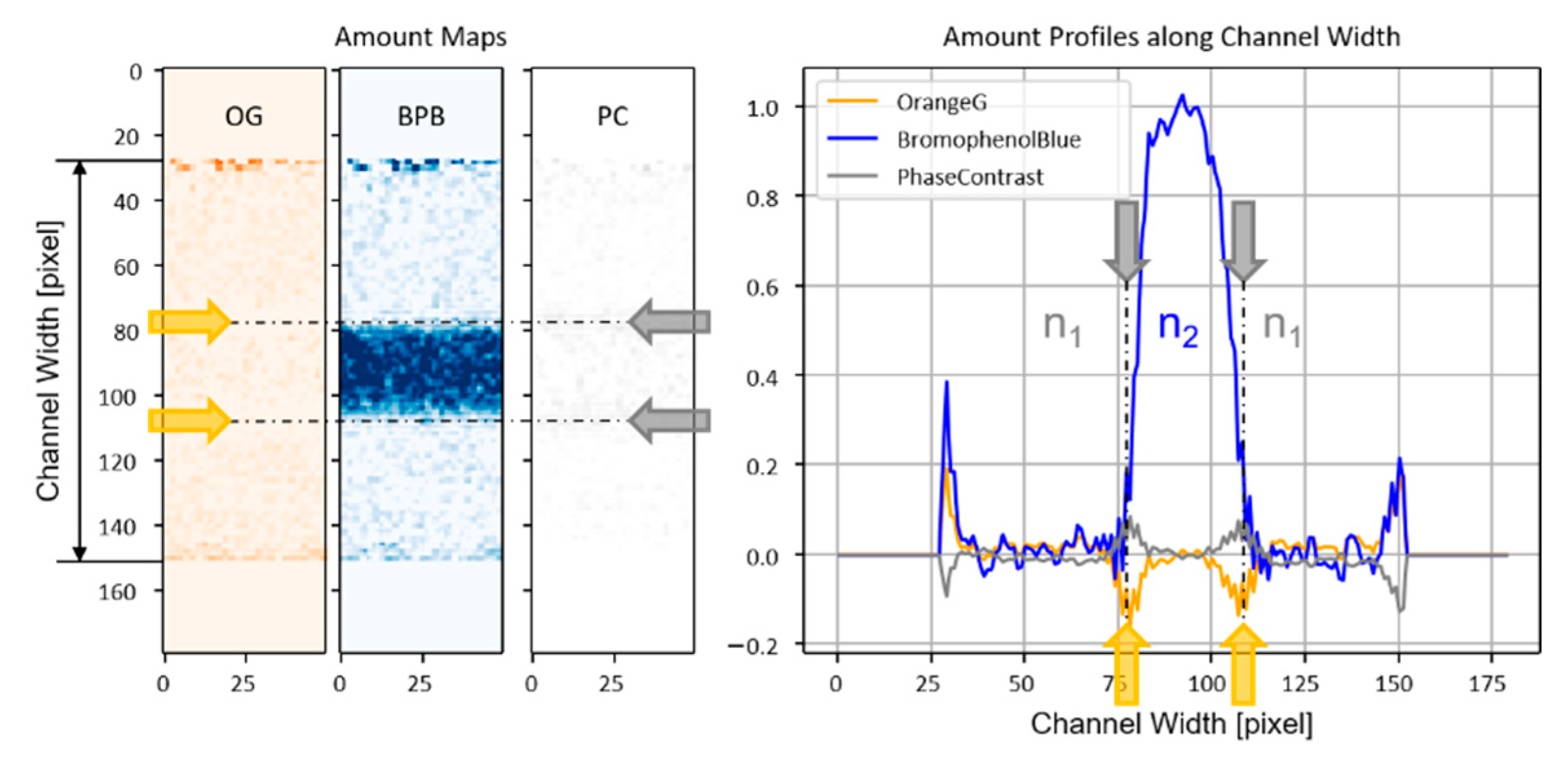
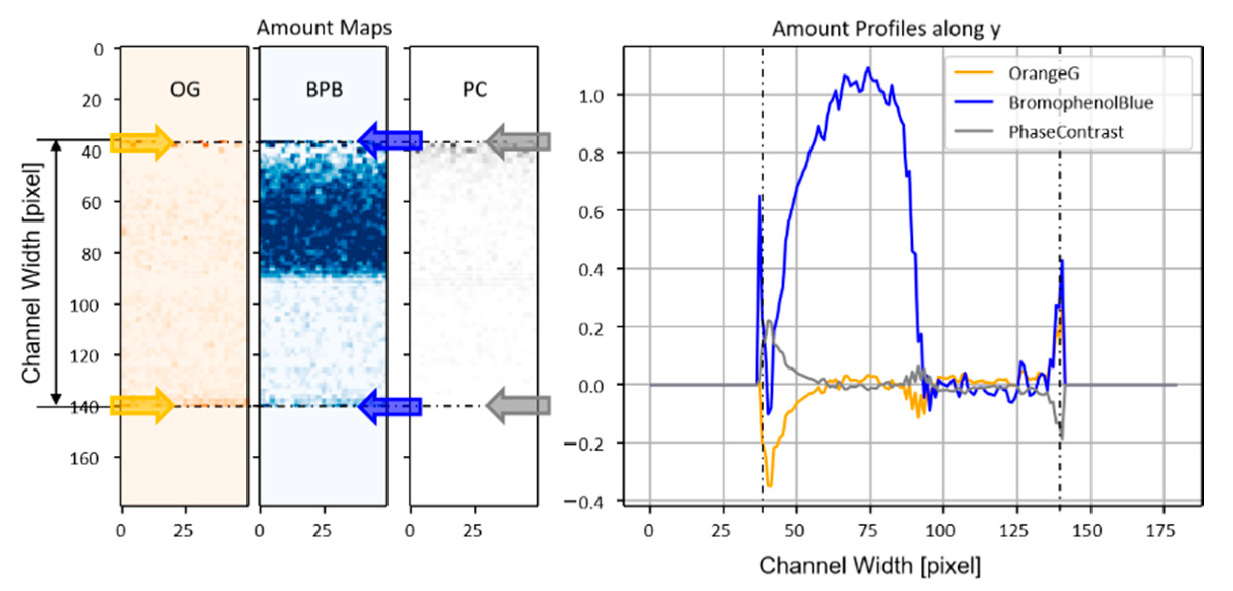
4.2.2. Single-Pixel Chemometric Analysis

For the quantitative chemometric analysis, the following quantities and definitions are utilized.

The area-related amount of substance N describes the amount of a pure component detected at a given area element. The physical meaning results from the Beer–Lambert Law in Equation (5) with

$$\mathrm{N} =\mathrm{c}\cdot \mathrm{d},$$

(7)

where c denominates a volumetric concentration and d the effective optical path length (NA > 0). The parameter can be interpreted as the amount of substance of a component, given in mol/m², detected by a single camera pixel. Per definition, the amount of a pure component detected for d = d_max, at the nominal channel height H, equals 1.

The phase fraction α_i denominates the fraction of a pure component i contained in a mixture of n components and is given by:

$${\mathsf{\alpha }}_{\mathrm{i}}=\frac{{\mathrm{N}}_{\mathrm{i}}}{{{\displaystyle \sum }}_{\mathrm{k}=0}^{\mathrm{n}}{\mathrm{N}}_{\mathrm{k}}}$$

(8)

Assuming a volumetric mixture of n components, the phase fraction α_i can also be calculated from the volume fractions V_i of the mixture. The same applies to the volume flow Q_i of pure components in a laminar co-flow scenario.

$${\mathsf{\alpha }}_{\mathrm{i}}=\frac{{\mathrm{V}}_{\mathrm{i}}}{{{\displaystyle \sum }}_{\mathrm{k}=1}^{\mathrm{n}}{\mathrm{V}}_{\mathrm{k}}}=\frac{{\mathrm{Q}}_{\mathrm{i}}}{{{\displaystyle \sum }}_{\mathrm{k}=1}^{\mathrm{n}}{\mathrm{Q}}_{\mathrm{k}}}$$

(9)

The measured RGB absorbance A_PIXEL:RGB of a single pixel reflects the absorbance of a mixture of the fluid components where each component i is characterized by unique spectral absorbance properties A_i:RGB. For analysis, we want to know the phase fraction α_i for each of the contributing components i. Therefore, we have the spectral properties of the pure components A_i.:RGB available as a reference. The observed single-pixel RGB absorbance spectrum A_OBS:RGB of a mixture of n pure components where each component contributes with an amount N_i is described by the following system of equations:

$$\left[\begin{array}{c}{\mathrm{A}}_{\mathrm{OBS}:\mathrm{R}}\\ {\mathrm{A}}_{\mathrm{OBS}:\mathrm{G}}\\ {\mathrm{A}}_{\mathrm{OBS}:\mathrm{B}}\end{array}\right]={\displaystyle \sum }_{\mathrm{i}=1}^{\mathrm{n}}{\mathrm{N}}_{\mathrm{i}}\left[\begin{array}{c}{\mathrm{A}}_{\mathrm{i}:\mathrm{R}}\\ {\mathrm{A}}_{\mathrm{i}:\mathrm{G}}\\ {\mathrm{A}}_{\mathrm{i}:\mathrm{B}}\end{array}\right]$$

(10)

A_OBS:RGB and A_i:RGB are retrieved from the measurements. Thus, Equation (10) can be solved to obtain Ni by the numerical solver for chemometric and spectral unmixing. The solver is based on a least-square method, which has been recently proposed and discussed by N. Coca [27].

RGB values are retrieved from single-pixel readout and converted to absorbance values A according to Equation (6). The area-related amount of substance N_i for the components is obtained from these RGB absorbances. For each pixel measurement, the phase fractions α_i for Bromophenol blue (‘BPB’), Orange G (‘OG’), and the water buffer (‘W’) fluid components are calculated from the respective amount N_i divided by the total amount N_T, exemplary demonstrated for ‘BPB’:

$${\mathsf{\alpha }}_{\mathrm{BPB}}=\frac{{\mathrm{N}}_{\mathrm{BPB}}}{{\mathrm{N}}_{\mathrm{T}}}=\frac{{\mathrm{N}}_{\mathrm{BPB}}}{{\mathrm{N}}_{\mathrm{BPB}}+{\mathrm{N}}_{\mathrm{OG}}+{\mathrm{N}}_{\mathrm{W}}}$$

(11)

The sum of phase fractions of the pure components accumulates to 1.0 for the respective component as the mixture analysis yields α_i for all the contributing components ‘OG’, ‘BPB’, and ‘W’:

$${\mathsf{\alpha }}_{\mathrm{OG}}+{ \mathsf{\alpha }}_{\mathrm{BPB}}+{\mathsf{\alpha }}_{\mathrm{W}}=1$$

(12)

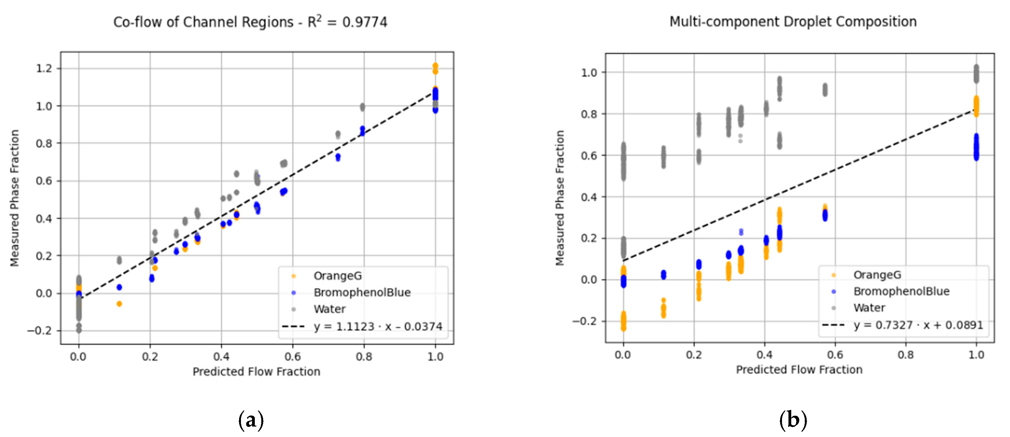
4.2.3. Accumulated Phase Fractions in a Channel

In the previous section, we have demonstrated the calculation of the phase fractions α_i for a single pixel measurement. For laminar co-flow experiments, the phase fractions α are measured for each acquired sample image at different channel positions. Therefore, the data are analyzed along measurement boxes, spanning the channel width, as illustrated in Figure 12. Box positions and dimensions can be specified for an arbitrary number of boxes.

The phase fraction is calculated by accumulation over all pixels of the box inside the channel. Due to the particular shape of our channels shown in Figure 12, the local channel height h(y) changes depending on the position. Thus, the optical path length d becomes a positional dependent variable. While the channel height h(y) can be calculated precisely from the known channel shape, the optical path length d is additionally influenced by the NA of the illumination and the refraction of the illumination beam at the curved channel walls. The prediction of these effects is challenging. Therefore, the effective optical path length d(y) is derived from the absorbance of the reference IM_FILLED, according to Equations (5) and (6), for a user-definable color-channel. To compensate for the variation of the channel height, d(y) is normalized towards maximum channel height d_max. Thus, the phase fraction α_i accumulated over the channel results in

$${\mathsf{\alpha }}_{\mathrm{i}}=\frac{1}{\left({\mathrm{y}}_2-{\mathrm{y}}_1\right)}{{\displaystyle \int }}_{{\mathrm{y}}_1}^{{\mathrm{y}}_2}\frac{{\mathrm{N}}_{\mathrm{i}}\left(\mathrm{y}\right)}{{\mathrm{N}}_{\mathrm{T}}\left(\mathrm{y}\right)}{\mathrm{dy} \mathrm{with} \mathrm{N}}_{\mathrm{T}}\left(\mathrm{y}\right)=\frac{1}{\mathrm{pixel} \mathrm{area}}\cdot \frac{\mathrm{d}\left(\mathrm{y}\right)}{{\mathrm{d}}_{\max }},$$

(13)

where y₁ and y₂ denominate the wall positions of the channel. The accumulated phase fractions α_i provide the phase fractions of all fluid components, passing through the channel at the boxed regions.

For comparison of the in-line image data and the mfnSolver model prediction, the phase fraction of each line over the channel is calculated analog to Equation (13), while the mfnSolver output takes the ratio of the sample flowrate over the total in-line flow rate of the respective channel. Five measurement boxes are distributed over the main channel length, as shown in Figure 12. The correlation of measured phase fractions with solver-predicted flow fractions is given in Figure 13a. A slope of 1.0 denominates the perfect fit. The figure shows good agreement between the measured phase fractions in the channel sections and the initially predicted flow settings from the mfnSolver, with a slope of 1.03 (R² = 0.97).

Details on the composition of the three-component co-flow for the individual subsets of the measurement and its relation to the mfnSolver predicted compositions are given in Figure 13b as a phase diagram. The predicted flow fractions show good agreement with the measured ones, and also their point of intersection almost coincides.

4.2.4. Validation of Predicted Flow Rates Based on Droplet Composition

In this section, the total flow rate of the dispersed phase and the continuous phase is kept constant, as shown in Figure 14 (top). Only the phase fractions of the dispersed phase are varied, as illustrated in Figure 14 (middle). The FOV with the respective measurement boxes and the region for droplet detection and measurement are shown in Figure 14 (bottom).

Boxes 1, 2, and 3 mentioned in Figure 14 (bottom) show a laminar co-flow, analyzed analogously to the previously described section. The correlation of the co-flow phase fractions compared to the predicted flow fractions show good agreement in Figure 15a, which fits the description in the previous section. However, it can be seen that the non-symmetric color-combination from the inlets leads to more outliers and higher deviations between the measured and calculated phase fractions from the ideal slope.

The droplet-flow phase fractions are calculated by accumulating all pixels inside a droplet using the scheme described for a box measurement. The droplet regions are detected by binarization of pre-processed input images with a given threshold, followed by filling the holes and eroding the binary mask to the inner volume of the droplets. The color components inside the drops are qualitatively analyzed. While the overall linearity can still be seen from the experimental data in Figure 15b, systematic deviations are observed, further discussed in the following section.

5. Precision of the Chemometric Analysis in Optofluidics

We confirm a straight correlation of the measured phase fractions with the solver predicted flow fractions in the measured data. At the same time, we recognize ‘color’-specific systematic deviations for the different colored fluids for the laminar co-flow patterns. For the measurements of the droplet contents, significantly higher deviations are observed. In general, image data acquisition is performed in transmission mode. Obviously, this raises the question of whether distortions of the optical beams during sample fluid and channel transmission may be assigned to these deviations. The following effects can be considered:

• Optical refraction at discrete refractive index transitions at the curved channel sidewalls;
• Optical refraction at dynamic refractive index changes at the boundary of the two fluid samples, with different refractive indices. Here, one has to note that adding a dye to a buffer changes its refractive index.
• Chromatic aberration (chromatic distortion) due to refraction, which applies to items 1 and 2.

These effects will influence the correctness of the measured transmitted optical path length of the fluid related to local channel heights and droplet heights. Furthermore, they may cause a shift in the spectral properties detected by the camera pixels at the affected positions, which leads to flawed absorbance spectra as the input for the chemometric analysis. The impact of these effects on the accuracy of the measured values can be assessed using intermediate data from the data processing chain available for each experiment.

A dynamic refractive index change at the boundary between ‘W’ (n₁) and ‘BPB’ (n₂) generates a curved dynamic refractive index transition. The resulting refraction is related to chromatic aberration and a shift in the detected spectral signatures for this region, which can be observed in Figure 16. These deviations lead to misleading results in the chemometric analysis. In this case, we observe false-positive amounts for the magnitudes of ‘OG’ and phase-contrast (‘PC’) with opposing signs, as indicated with the arrows in Figure 16. The chemometric analysis was performed for the amounts of ‘OG’ and ‘BPB’ and ‘PC’, where the absorbance values for the pure phase-contrast are considered as A_PC:RGB = [1.0 1.0 1.0], assuming uniform contrast for all color-channels.

The curved shape of the channel sidewalls results in refraction and chromatic aberration, leading to false amounts of the components at near-wall positions, as shown in Figure 17. The valid area of analysis is the center of the channel. In addition, we observe an alternating sign of the deviation, which might be related to an alignment error of the illumination beam to the optical axis of the imaging system.

The same combination of refraction and chromatic aberration is observed in proximity to the curved interface of the investigated droplets, as illustrated in Figure 18. The refractive index change between the continuous oil phase and the droplet components enhances these optical effects.

All these effects are contributing to the correctness of the measured values. They could be outbalanced by using refractive index-matched special fluids, as proposed by D. Malsch [23]. However, these special fluids are incompatible with any biological assay or chemical reaction. Therefore, the decision was made towards fluid compositions, typical for a broad range of biological and molecular biology assays, such as Phosphate Buffer at pH 8.0 and perfluorinated oils for droplet experiments. The results of this section demonstrate how optofluidic effects are related to the quality and precision of the on-chip chemometric measurements and are intended to provide valuable hints for implementing these measurement approaches in real lab-on-a-chip applications.

6. Discussion and Outlook

While much work has already been done towards microfluidic design automation [13,16,17,18] and control, to our knowledge, a general and easily implementable solution is still unavailable to the community. The developed mfnSolver can be understood as one core component of the MDA architecture, which provides a reliable system simulation for the fast and iterative optimization of microfluidic networks. Thus, it is applicable for the design of lab-on-a-chip systems and the in-line prediction of the correct settings for their operation.

For implementing the microfluidic network graph of a particular chip design, it might be difficult to exactly access and measure the geometrical parameters of commercially available microfluidic devices. However, the mfnSolver is comparably robust to length variations, as long as the majority of the pressure drop can be assigned to the interconnecting tubes. For example, a variation of four mm at different positions of the on-chip network only leads to an average difference across pressure predictions of 2.337 mbar with a sample standard deviation of 0.364 mbar. On the one hand, the solver calculates the hydrodynamic resistance as displayed in Equation (3). Thus, the length is only factored in once in the nominator of the equation.

On the other hand, if the network is designed so that the main pressure drop occurs along the feedlines, the network behavior is dominated by the throughput characteristics of the interconnecting system. In this case, the Kirchhoff-graphs show that only less than 5% of the pressure drop across the entire system drops over the microfluidic chip itself. The most significant pressure drop is contributed by the capillaries connecting the microfluidic control with the chip. The respective manufacturer usually provides measures of the inner diameter of the capillaries. It is also the crucial parameter in calculating the hydraulic diameter, which appears with a power of four in Equation (3). Exemplarily, a variation of 20 µm across the four capillaries can lead to a deviation of over 15% of the pressure output provided by the solver. Therefore, it is necessary to calibrate the inner diameter of the capillaries before usage.

While we only present the mfnSolver for applications utilizing pressure-driven flow control, the solver is not limited to this application range. The mfnSolver can be further applied to iterative MFN design optimizations to tailor on-chip channel characteristics to meet desired control parameters. Furthermore, several networks can be implemented into the solver and stitched together to analyze and simulate parallel operation. Due to the high computational speed, the mfnSolver can be easily integrated into closed-loop control applications.

7. Final Conclusions

In this work, we confirmed the outstanding potential of the microfluidic network solver (mfnSolver) as a reliable tool for fast and precise prediction of pressure settings for steady-state operation conditions and getting insights into on-chip pressure drop and flow characteristics. In contrast to common CFD analyzers, the mfnSolver can analyze a complete microfluidic network within a few milliseconds. The mfnSolver can be implemented and tailored based on the chip fabrication parameters, etch depth, mask width, and on-chip lengths between the defined nodes and available microfluidic control units. It precisely predicts the operation parameters for laminar co-flow and droplet operation within the established microfluidic framework.

Furthermore, the solver has been experimentally validated to create and analyze laminar co-flow and droplets with systematically variable compositions. In combination with chemometric analysis, absorbance imaging has been found as a precise and contactless optical method for quantitative monitoring of transport processes in microfluidic devices. The impact of optofluidic effects on the precision of the chemometric analysis has been discussed.

References

1. Huebner, A.; Sharma, S.; Srisa-Art, M.; Hollfelder, F.; Edel, J.B.; Demello, A.J. Microdroplets: A sea of applications? Lab Chip 2008, 8, 1244–1254. [Google Scholar] [CrossRef] [PubMed]
2. Guenther, A.; Jensen, K.F. Multiphase microfluidics: From flow characteristics to chemical and materials synthesis. Lab Chip 2006, 6, 1487–1503. [Google Scholar] [CrossRef] [PubMed]
3. Fan, Y.-Q.; Wang, M.; Gao, F.; Zhuang, J.; Tang, G.; Zhang, Y.-J. Recent Development of Droplet Microfluidics in Digital Polymerase Chain Reaction. Chin. J. Anal. Chem. 2016, 44, 1300–1307. [Google Scholar] [CrossRef]
4. Fallahi, H.; Zhang, J.; Phan, H.-P.; Nguyen, N.-T. Flexible Microfluidics: Fundamentals, Recent Developments, and Applications. Micromachines 2019, 10, 830. [Google Scholar] [CrossRef] [Green Version]
5. Geng, Y.; Ling, S.; Huang, J.; Xu, J. Multiphase Microfluidics: Fundamentals, Fabrication, and Functions. Small 2020, 16, e1906357. [Google Scholar] [CrossRef] [PubMed]
6. Sun, K.; Wang, Z.; Jiang, X. Modular microfluidics for gradient generation. Lab Chip 2008, 8, 1536–1543. [Google Scholar] [CrossRef] [PubMed]
7. Wang, X.; Liu, Z.; Pang, Y. Concentration gradient generation methods based on microfluidic systems. RSC Adv. 2017, 7, 29966–29984. [Google Scholar] [CrossRef] [Green Version]
8. Liu, Z.; Fontana, F.; Python, A.; Hirvonen, J.T.; Santos, H.A. Microfluidics for Production of Particles: Mechanism, Methodology, and Applications. Small 2019, 16, e1904673. [Google Scholar] [CrossRef]
9. Jahn, A.; Reiner, J.E.; Vreeland, W.N.; De Voe, N.L.; Locascio, L.E.; Gaitan, M. Preparation of nanoparticles by continuous-flow microfluidics. J. Nanopart. Res. 2008, 10, 925–934. [Google Scholar] [CrossRef]
10. Thiele, M.; Knauer, A.; Malsch, D.; Csáki, A.; Henkel, T.; Köhler, J.M.; Fritzsche, W. Combination of microfluidic high-throughput production and parameter screening for efficient shaping of gold nanocubes using Dean-flow mixing. Lab Chip 2017, 17, 1487–1495. [Google Scholar] [CrossRef] [PubMed]
11. Gomez, F.A. The future of microfluidic point-of-care diagnostic devices. Bioanalysis 2013, 5, 1–3. [Google Scholar] [CrossRef] [PubMed]
12. Reuter, C.; Hentschel, S.; Breitenstein, A.; Heinrich, E.; Aehlig, O.; Henkel, T.; Csáki, A.; Fritzsche, W. Chip-based duplex real-time PCR for water quality monitoring concerning Legionella pneumophila and Legionella spp. Water Environ. J. 2021, 35, 371–380. [Google Scholar] [CrossRef]
13. Tsur, E.E. Computer-Aided Design of Microfluidic Circuits. Annu. Rev. Biomed. Eng. 2020, 22, 285–307. [Google Scholar] [CrossRef] [PubMed]
14. Kielpinski, M.; Walther, O.; Cao, J.; Henkel, T.; Köhler, J.M.; Groß, G.A. Microfluidic Chamber Design for Controlled Droplet Expansion and Coalescence. Micromachines 2020, 11, 394. [Google Scholar] [CrossRef] [PubMed] [Green Version]
15. Feinerman, O.; Sofer, M.; Tsur, E.E. Computer-Aided Design of Valves-Integrated Microfluidic Layouts Using Parameter-Guided Electrical Models. In Proceedings of the Fluids Engineering Division Summer Meeting in Montreal, Montreal, QC, Canada, 15–20 July 2018; American Society of Mechanical Engineers Digital Collection: New York, NY, USA, 2018. [Google Scholar]
16. Lee, K.; Kim, C.; Ahn, B.; Panchapakesan, R.; Full, A.R.; Nordee, L.; Kang, J.Y.; Oh, K.W. Generalized serial dilution module for monotonic and arbitrary microfluidic gradient generators. Lab Chip 2009, 9, 709–717. [Google Scholar] [CrossRef]
17. Oh, K.W.; Lee, K.; Ahn, B.; Furlani, E.P. Design of pressure-driven microfluidic networks using electric circuit analogy. Lab Chip 2012, 12, 515–545. [Google Scholar] [CrossRef] [PubMed]
18. Gleichmann, N.; Malsch, D.; Horbert, P.; Henkel, T. Toward microfluidic design automation: A new system simulation toolkit for the in silico evaluation of droplet-based lab-on-a-chip systems. Microfluid. Nanofluid. 2015, 18, 1095–1105. [Google Scholar] [CrossRef]
19. Seemann, R.; Brinkmann, M.; Pfohl, T.; Herminghaus, S. Droplet based microfluidics. Rep. Prog. Phys. 2012, 75, 16601. [Google Scholar] [CrossRef]
20. Garstecki, P.; Fuerstman, M.J.; Stone, H.A.; Whitesides, G.M. Formation of droplets and bubbles in a microfluidic T-junction—scaling and mechanism of break-up. Lab Chip 2006, 6, 437–446. [Google Scholar] [CrossRef]
21. Akers, A.; Gassman, M.; Smith, R.J. Hydraulic Power System Analysis; CRC/Taylor & Francis: Boca Raton, FL, USA, 2006; ISBN 0824799569. [Google Scholar]
22. Tsur, E.E.; Zimerman, M.; Maor, I.; Elrich, A.; Nahmias, Y. Microfluidic Concentric Gradient Generator Design for High-Throughput Cell-Based Studies. Front. Bioeng. Biotechnol. 2017, 5, 21. [Google Scholar] [CrossRef] [Green Version]
23. Kirchhoff, S. Ueber den Durchgang eines elektrischen Stromes durch eine Ebene, insbesondere durch eine kreisförmige. Ann. Phys. 1845, 140, 497–514. [Google Scholar] [CrossRef] [Green Version]
24. Henkel, T.; Bermig, T.; Kielpinski, M.; Grodrian, A.; Metze, J.; Köhler, J. Chip modules for generation and manipulation of fluid segments for micro serial flow processes. Chem. Eng. J. 2004, 101, 439–445. [Google Scholar] [CrossRef]
25. Wuest, W. Strömung durch Schlitz- und Lochblenden bei kleinen Reynolds-Zahlen. Ing. Archiv 1954, 22, 357–367. [Google Scholar] [CrossRef]
26. Malsch, D.; Kielpinski, M.; Gleichmann, N.; Mayer, G.; Henkel, T. Reconstructing the 3D shapes of droplets in glass microchannels with application to Bretherton’s problem. Exp. Fluids 2014, 55, 1841. [Google Scholar] [CrossRef]
27. Coca, N. A Classical Least Squares Method for Quantitative Spectral Analysis with Python. Towards Data Science. 13 April 2020. Available online: https://towardsdatascience.com/classical-least-squares-method-for-quantitative-spectral-analysis-with-python-1926473a802c (accessed on 26 May 2021).
Figure 1. (a) Quality of the pressure control as a correlation of the pressure setting and the average pressure displayed by the control unit, with a correlation coefficient R2 = 0.9987; (b) quality of flow sensors as a correlation of the expected flow rate for the weight out fluid against the average display of the calibrated flow sensors (R2 = 0.9969).
Processes 09 01320 g001
Figure 2. (a) Pressure-throughput performance of 500.0 mm long PEEK capillaries; (b) calculated mean inner diameter for each capillary with its standard error and nominal inner diameter for comparison. The overall mean inner diameter of all capillaries is 0.136 mm.
Processes 09 01320 g002
Figure 3. Schematic representation of the solver concept and its purpose.
Processes 09 01320 g003
Figure 4. (a) Conceptual demonstration of the MFC and a symmetrical on-chip network; (b) representative Kirchhoff-graph with ports Pi, nodes Ni, and edges Ei for the MFC tubing with the respective on-chip parameters; (c) Translation to the respective system of linear equations with the incidence matrix MI.
Processes 09 01320 g004
Figure 5. (a) Implementation of the mfnSolver in numeric Python with class hierarchy and aggregation. Solving the system of linear equations using numerical Python; (b) representative Kirchhoff-graph solved with the mfnSolver.
Processes 09 01320 g005
Figure 6. Channel cross-section of the utilized PDG2 microfluidic device. The ports are defined according to the D-sub nomenclature, with P1, P2, P3, P5 as inlets and P4 as the outlet.
Processes 09 01320 g006
Figure 7. (a) The central flow-focusing unit (FFU) geometry of the PDG2 chip for the lower half channel. The color scheme encodes the wall distance from the center plane at z = 0. The utilization of the FFU for droplet generation benefits from the integration of sharp-edged apertures, which can be managed by isotropic wet etching technology [25]. The arrow is indicating the main channel flow direction. The sheet flow is applied from the lateral channel branches; (b) the parameter MW and ED refer to the utilized mask width (MW) and the uniform etch depth (ED), and W and H denominate the final channel width and height. The channel width W varies over the internal channel sections of the chip.
Processes 09 01320 g007
Figure 8. mfnSolver output with predicted pressure settings for the feedlines to create laminar co-flow in the PDG2 chip device (top) (complete mfnSolver output in (top) and in more detail in Figure S1: mfnSolver output Kirchhoff-graph co-flow); mfnSolver output with predicted pressure settings for the feedlines to create multi-component droplet flow in the PDG2 chip device (bottom) (also see Figure S2: mfnSolver output Kirchhoff-graph droplet flow).
Processes 09 01320 g008
Figure 9. Experimental parameter space and corresponding IDs for laminar co-flow. Variation of the total flowrate QT throughout the pressure profiles (top); output composition of the laminar co-flow components over the different parameter settings (middle); experimental FOV for pressure parameter set ID 1, with port P1 containing the Orange G (‘OG’) dye solution fed with 50 mbar while all remaining ports P2, P3, and P5 are operated at the standard pressure of 100 mbar (bottom).
Processes 09 01320 g009
Figure 10. Correlation of pressure settings, predicted by the mfnSolver, with experimental results. A slope value of 1 indicates perfect matching. (a) Pressure-throughput performance during the experiment (blue) and the laminar co-flow model prediction (orange) with a correlation coefficient R2 = 0.9985; (b) pressure-throughput performance during the experiment (blue) and the droplet-flow model prediction (orange) with a correlation coefficient (R2 = 0.9909).
Processes 09 01320 g010
Figure 11. Experimental field of view for droplet-flow. A laminar flow pattern is created as the dispersed phase. The input pressure of the continuous phase channel at P1 is kept constant at 900 mbar. (a) The remaining channels are fed with 100 mbar through P5 and 175 mbar through P2 and P3; (b) all remaining channels connected to the operating pressure of 150 mbar each; (c) P5 is fed with 200 mbar, P2 and P3 are operated with 125 mbar.
Processes 09 01320 g011
Figure 12. Generation of a laminar co-flow from the fluid components ‘BPB’, ‘W’, and ‘OG’ in a PDG2 Flow-Focusing Chip device. White boxes indicate the chosen measurement positions for the optical readout of concentration profiles. Arrows indicate the flow direction.
Processes 09 01320 g012
Figure 13. Correlation of measured and predicted phase fractions of the created laminar co-flow pattern at different chip-internal channel sections (see Figure 12). A slope value of 1 indicates perfect matching—the central flow-focusing correlation of the measured phase fraction with the predicted flow fraction values from the mfnSolver. (a) The correlation of measured phase fraction and predicted flow rates of a laminar co-flow over the investigated channel regions show a correlation coefficient R2 = 0.97. The straight linear correlation has a slope of 1.03 and an intersection at −0.01; (b) the phase diagram indicates matching the predicted flow composition and the actual color pattern for regions 4 and 5 after the FFU.
Processes 09 01320 g013
Figure 14. Experimental parameter space and corresponding IDs for multi-component droplet-flow. The total flowrate QT is kept constant throughout the pressure profiles (top); output composition of the color-components of the laminar co-flow components over the different parameter settings (middle); experimental FOV for pressure parameter set ID 1, with port P1 containing the continuous phase fed with 900 mbar while all remaining ports P2 (‘OG’), P3 (‘BPB’), each operated at 175 mbar and P5 (‘W’) operated at 100 mbar (bottom). The combined pressure of the laminar components is set to 450 mbar.
Processes 09 01320 g014
Figure 15. Correlation of measured and predicted phase fractions for droplet operation (a) in the channel section with a slope of 1.11 (R2 = 0.98); (b) the multi-component composition inside the droplets, with a slope of 0.73 and an intersection at 0.09.
Processes 09 01320 g015
Figure 16. Chemometric analysis of a two-component laminar co-flow of water with a centered lamella of ‘BPB’. Amount maps spanning over the channel width for the three components ‘OG’, ‘BPB’, and ‘PC’ (left); Quantitative amount profiles of the fluid components and respective refractive index regions ni (right).
Processes 09 01320 g016
Figure 17. Chemometric analysis of a two-component laminar co-flow of water and ‘BPB’. Amount maps spanning over the channel width for the three components ‘OG’, ‘BPB’ and ‘PC’ (left); quantitative amount profiles of the fluid components showing near-wall effects (right).
Processes 09 01320 g017
Figure 18. Chemometric analysis of a three-component droplet. (a) Quantitative amount maps; (b) amount profile over the droplet width y.
Processes 09 01320 g018