Effective Similarity Variables for the Computations of MHD Flow of Williamson Nanofluid over a Non-Linear Stretching Surface

Abstract

The present study concerns investigating the two-dimensional Magnetohydrodynamics (MHD) boundary layer flow of Williamson nanofluid over a non-linear stretching sheet. The focus of this study is based on the global influence of the non-Newtonian Williamson fluid parameter $\left(\lambda \right)$ rather than the local one that exists in the literature for linear and non-linear stretching cases. The mathematical model of the problem is based on the law of conservation of mass, momentum, and energy. The derived partial differential equations are transformed into ordinary differential equations by applying an appropriate similarity transformation. The subsequent equations are solved numerically by using the Shooting method. The physical quantities Skin friction coefficient, as well as the Sherwood and Nusselt numbers are computed locally. To validate the implemented shooting method, a comparison is made with the results obtained by Matlab function bvp4c, and good agreement is found. The Prandtl number, $Pr$, has an increasing impact of 25.14% on the wall temperature gradient. The impact of various physical parameters are presented through graphs and tables.

1. Introduction

The two main categories of fluid mechanics are Newtonian and non-Newtonian fluid. The relationship among strain rate is described by deriving the constitutive equation, especially for those fluids that do not maintain the Newtonian law of viscosity. Several researchers have provided mathematical models to determine the rheological properties of such fluids. The models include the power-law, Williamson fluid, Ellis, cross, and Carreau models. Williamson [1] provided the Williamson model for pseudoplastic materials, which is an experimentally verified model. The characteristic of the Williamson fluid model involves choosing minimum $\left({\mu }_0\right)$ and maximum $\left({\mu }_{\infty }\right)$ viscosity at the same time. In real fluid, minimum as well as maximum viscosity is needed for the mathematical model. Pseudoplastic fluids are commonly used in industry as melts of high molecular weight polymer solution, photographic film, and extrusion of polymer sheets [2]. Carmer et al. [3] investigated polymer solution using the Williamson fluid model. Lyubimov and Perminov [4] deliberated the flow of Williamson fluid over an inclined wall, with aspects of the gravitational field. Nadeem et al. [5] investigated the numerical solution of the peristaltic flow of Williamson fluid by radially varying MHD in an endoscope. Noreen Sher Akbar et al. [6] used the Carreau model and Ismail et al. [7] used the power-law model to investigate flow of blood in arteries. Ahmed et al. [8] numerically scrutinized the impact of Williamson fluid flow over an exponential stretching surface. Ramzan et al. [9] performed linear analysis of heat transfer in three-dimensional Williamson nanofluid with a Cattaneo-Christov heat flux model.

In the industrial process, liquids’ thermal features play an essential role in requirements such as in heating and cooling [10,11,12,13]. The transfer of heat performance of a liquid is regulated by its thermal conductivity. Furthermore, fluids’ thermal conductivity via water, engine oil, and ethylene glycol is inherently low compared to that of solids [14,15]. Researchers have tried to escalate the thermal conductivity of such conventional heat transfer fluids using tiny particles of solids with high thermal conductivity. Many researchers have investigated the millimeter and micrometer dimensions of these solid suspensions, and significant drawbacks such as low thermal conductivity, particle sedimentation, excessive pressure drops, particle clogging, etc., were observed. By downsizing the particle size, the performance of heat transfer is improved in liquids [16,17,18,19,20,21]. With nanotechnology advancements, scientists on an atomic or molecular scale prepared a nanometer-sized particle with enhanced thermo-physical properties [22,23,24,25,26]. In a base fluid, the suspension of nanoparticles is known as nanofluid. It has been experimentally proven the nanofluid’s thermal conductivity is higher than for base fluids. Inside the base fluid, the nanoparticles easily fluidize, due to which sedimentation and clogging of channels are no longer problems.

The heat transfer and the boundary layer flow over a stretching sheet are essential in engineering and industries due to their many applications [27,28,29,30,31,32,33,34]. At the final stage of processing, the final products’ characteristics are highly dependent upon stretching and heat transfer rate. Under several stretching velocities, different natural processes take place. Such flow situations are encountered in numerous manufacturing processes, like polymer sheet production, extrusion from dye metal spinning, rubber sheet production, glass blowing, paper product manufacturing, annealing of copper wires and glass fiber, etc. Sakiadis [35,36,37] discussed the impact of constant velocity on Newtonian fluid due to a moving plate. The two-dimensional steady flow over a stretching linear surface was established for the first time by Crane [38]. Numerous authors further extended Crane’s work by considering several physical phenomena, like the influence of the magnetic field, injection or suction, and heat transfer effects on such flow caused by a stretched surface. Gupta [39] investigated the stretching flow along with suction/injection. The influence of linear velocity on stretching/shrinking walls and consideration of hydromagnetic, chemical reaction, and viscous dissipation have been studied by Kameswaran [40]. Khan et al. [41] used an optimal homotopy analysis method to investigate heat transfer in a boundary layer nanofluid equipped with a Cattaneo-Christov heat flux model over an exponentially stretching surface.

MHD flows have fundamental importance from a scientific and applied point of view. The study involves the consideration of an applied magnetic field on the flow of electrically conducting fluid. The subject has developed to such an extent that it is not possible to refer to even a fraction of the literature and its applications. However, recognizing its importance, we will introduce MHD effects in the stretching phenomenon for non-Newtonian Williamson fluid. Some relevant background literature of interest will help to understand its significance for our purposes. The study of MHD flows induct theoretical and experimental work, which Hartmann and Lazarus performed. MHD has many applications in fields such as fusion reactors (blanket, diverter, limiter, F.W.), astrophysics (planetary magnetic field), crystal growth, ship propulsion, dispersion (granulation) of metals, jet printers, MHD pumps (1907), MHD flow meters (1935), MHD generators (1923), metallurgy (induction furnace as well as the casting of Al and Fe), magnetic filtration and separation, and MHD flow control (reducing turbulent drag) [42,43,44,45,46]. Hussain et al. [47] used the Keller box method to investigate the MHD convective flow of Williamson fluid with homogeneous-heterogeneous reactions.

The present paper aims to examine the influence of MHD Williamson nanofluid flow over a non-linear stretching sheet. The focus of this study is based on the global influence of the Non-Newtonian Williamson fluid parameter rather than the local one. To the best of the authors’ knowledge, the proposed model on similarity transformation has not yet been considered. The governing non-linear PDEs are reduced into the system of non-linear ODEs with the help of similarity transformation. The transformed equations are numerically solved by applying the shooting method and bvp4c. The dimensionless skin friction, wall temperature gradient, and Sherwood number are obtained and are displayed in

Table 1. Effect of physical parameters on the skin friction coefficient.

$\mathit{\lambda }\downarrow$	$\mathit{M}\uparrow$	$\mathit{P}\mathit{r}$	$\mathit{N}\mathit{b}\mathit{t}$	$\mathit{N}\mathit{c}$	$\mathit{L}\mathit{e}$	$\mathit{S}\mathit{c}$	$-\left({\mathit{f}}^{″}\left(0\right)+\frac{\mathit{\lambda }}{6}{{\mathit{f}}^{″}}^2\left(0\right)\right)$
							Shooting Method	bvp4c
0.1	$0.5$	$0.5$	$2.0$	$0.5$	$3.0$	$2.0$	$0.786446$	$0.786446$
0.2	$0.5$	$0.5$	$2.0$	$0.5$	$3.0$	$2.0$	$0.782473$	$0.782473$
$0.3$	$0.5$	$0.5$	$2.0$	$0.5$	$3.0$	$2.0$	$0.778424$	$0.778424$
$0.5$	$0.1$	$0.5$	$2.0$	$0.5$	$3.0$	$2.0$	$0.694890$	$0.694890$
$0.5$	$0.2$	$0.5$	$2.0$	$0.5$	$3.0$	$2.0$	$0.716547$	$0.716547$
$0.5$	$0.3$	$0.5$	$2.0$	$0.5$	$3.0$	$2.0$	$0.737670$	$0.737670$

,

Table 2. Effect of physical parameters on Nusselt number $-{\theta }^{\prime } \left(0\right)$.

$\mathit{\lambda }\downarrow$	$\mathit{M}\downarrow$	$\mathit{P}\mathit{r}\uparrow$	$\mathit{N}\mathit{b}\mathit{t}\uparrow$	$\mathit{N}\mathit{c}\downarrow$	$\mathit{L}\mathit{e}\uparrow$	$\mathit{S}\mathit{c}$	$-{\theta }^{\prime }\left(0\right)$
							Shooting Method	bvp4c
$0.1$	$0.5$	$0.5$	$2.0$	$0.5$	$3.0$	$2.0$	$0.288735$	$0.288735$
$0.2$	$0.5$	$0.5$	$2.0$	$0.5$	$3.0$	$2.0$	$0.288369$	$0.288369$
$0.3$	$0.5$	$0.5$	$2.0$	$0.5$	$3.0$	$2.0$	$0.287995$	$0.287995$
$0.5$	$0.1$	$0.5$	$2.0$	$0.5$	$3.0$	$2.0$	$0.294560$	$0.294560$
$0.5$	$0.2$	$0.5$	$2.0$	$0.5$	$3.0$	$2.0$	$0.292823$	$0.292823$
$0.5$	$0.3$	$0.5$	$2.0$	$0.5$	$3.0$	$2.0$	$0.291151$	$0.291151$
$0.5$	$0.5$	$0.1$	$2.0$	$0.5$	$3.0$	$2.0$	$0.189510$	$0.189510$
$0.5$	$0.5$	$0.2$	$2.0$	$0.5$	$3.0$	$2.0$	$0.212828$	$0.212828$
$0.5$	$0.5$	$0.3$	$2.0$	$0.5$	$3.0$	$2.0$	$0.237148$	$0.237148$
$0.5$	$0.5$	$0.5$	$0.4$	$0.5$	$3.0$	$2.0$	$0.249286$	$0.249286$
$0.5$	$0.5$	$0.5$	$0.5$	$0.5$	$3.0$	$2.0$	$0.258448$	$0.258448$
$0.5$	$0.5$	$0.5$	$0.6$	$0.5$	$3.0$	$2.0$	$0.264741$	$0.264740$
$0.5$	$0.5$	$0.5$	$2.0$	$0.1$	$3.0$	$2.0$	$0.326417$	$0.326417$
$0.5$	$0.5$	$0.5$	$2.0$	$0.2$	$3.0$	$2.0$	$0.316415$	$0.316415$
$0.5$	$0.5$	$0.5$	$2.0$	$0.3$	$3.0$	$2.0$	$0.306681$	$0.306681$
$0.5$	$0.5$	$0.5$	$2.0$	$0.5$	$0.3$	$2.0$	$0.062628$	$0.062628$
$0.5$	$0.5$	$0.5$	$2.0$	$0.5$	$0.4$	$2.0$	$0.097528$	$0.097528$
$0.5$	$0.5$	$0.5$	$2.0$	$0.5$	$0.5$	$2.0$	$0.126389$	$0.126389$
$0.5$	$0.5$	$0.5$	$2.0$	$0.5$	$3.0$	$0.1$	$0.304255$	$0.304254$
$0.5$	$0.5$	$0.5$	$2.0$	$0.5$	$3.0$	$0.2$	$0.302944$	$0.302944$
$0.5$	$0.5$	$0.5$	$2.0$	$0.5$	$3.0$	$0.3$	$0.301662$	$0.301662$

and

Table 3. Effect of physical parameters on Sherwood number $-g^{\prime } \left(0\right)$.

$\mathit{\lambda }\downarrow$	$\mathit{M}\downarrow$	$\mathit{P}\mathit{r}\downarrow$	$\mathit{N}\mathit{b}\mathit{t}\uparrow$	$\mathit{N}\mathit{c}\uparrow$	$\mathit{L}\mathit{e}\downarrow$	$\mathit{S}\mathit{c}\uparrow$	$-{\mathit{g}}^{\prime }\left(0\right)$
							$\mathbf{S}\mathbf{h}\mathbf{o}\mathbf{o}\mathbf{t}\mathbf{i}\mathbf{n}\mathbf{g} \mathbf{M}\mathbf{e}\mathbf{t}\mathbf{h}\mathbf{o}\mathbf{d}$	$\mathbf{b}\mathbf{v}\mathbf{p}4\mathbf{c}$
$0.1$	$0.5$	$0.5$	$2.0$	$0.5$	$3.0$	$2.0$	$0.693244$	$0.693243$
$0.2$	$0.5$	$0.5$	$2.0$	$0.5$	$3.0$	$2.0$	$0.692233$	$0.692232$
$0.3$	$0.5$	$0.5$	$2.0$	$0.5$	$3.0$	$2.0$	$0.691192$	$0.691191$
$0.5$	$0.1$	$0.5$	$2.0$	$0.5$	$3.0$	$2.0$	$0.707605$	$0.707604$
$0.5$	$0.2$	$0.5$	$2.0$	$0.5$	$3.0$	$2.0$	$0.703351$	$0.703351$
$0.5$	$0.3$	$0.5$	$2.0$	$0.5$	$3.0$	$2.0$	$0.699200$	$0.69920$
$0.5$	$0.5$	$0.1$	$2.0$	$0.5$	$3.0$	$2.0$	$0.739933$	$0.739933$
$0.5$	$0.5$	$0.2$	$2.0$	$0.5$	$3.0$	$2.0$	$0.727616$	$0.727615$
$0.5$	$0.5$	$0.3$	$2.0$	$0.5$	$3.0$	$2.0$	$0.715347$	$0.715346$
$0.5$	$0.5$	$0.5$	$0.4$	$0.5$	$3.0$	$2.0$	$0.591692$	$0.591691$
$0.5$	$0.5$	$0.5$	$0.5$	$0.5$	$3.0$	$2.0$	$0.604384$	$0.604383$
$0.5$	$0.5$	$0.5$	$0.6$	$0.5$	$3.0$	$2.0$	$0.617227$	$0.617226$
$0.5$	$0.5$	$0.5$	$2.0$	$0.1$	$3.0$	$2.0$	$0.675000$	$0.675000$
$0.5$	$0.5$	$0.5$	$2.0$	$0.2$	$3.0$	$2.0$	$0.679217$	$0.679216$
$0.5$	$0.5$	$0.5$	$2.0$	$0.3$	$3.0$	$2.0$	$0.683319$	$0.683318$
$0.5$	$0.5$	$0.5$	$2.0$	$0.5$	$0.3$	$2.0$	$0.788938$	$0.788937$
$0.5$	$0.5$	$0.5$	$2.0$	$0.5$	$0.4$	$2.0$	$0.772636$	$0.772635$
$0.5$	$0.5$	$0.5$	$2.0$	$0.5$	$0.5$	$2.0$	$0.759863$	$0.759862$
$0.5$	$0.5$	$0.5$	$2.0$	$0.5$	$3.0$	$0.1$	$0.172203$	$0.172204$
$0.5$	$0.5$	$0.5$	$2.0$	$0.5$	$3.0$	$0.2$	$0.198512$	$0.198513$
$0.5$	$0.5$	$0.5$	$2.0$	$0.5$	$3.0$	$0.3$	$0.225899$	$0.225899$

. The influence of the magnetic parameter, Prandtl number, diffusivity parameter, Williamson fluid parameter, Schmidt number, Lewis number, and heat capacity ratio on velocity, temperature, and concentration profiles are shown through graphs.

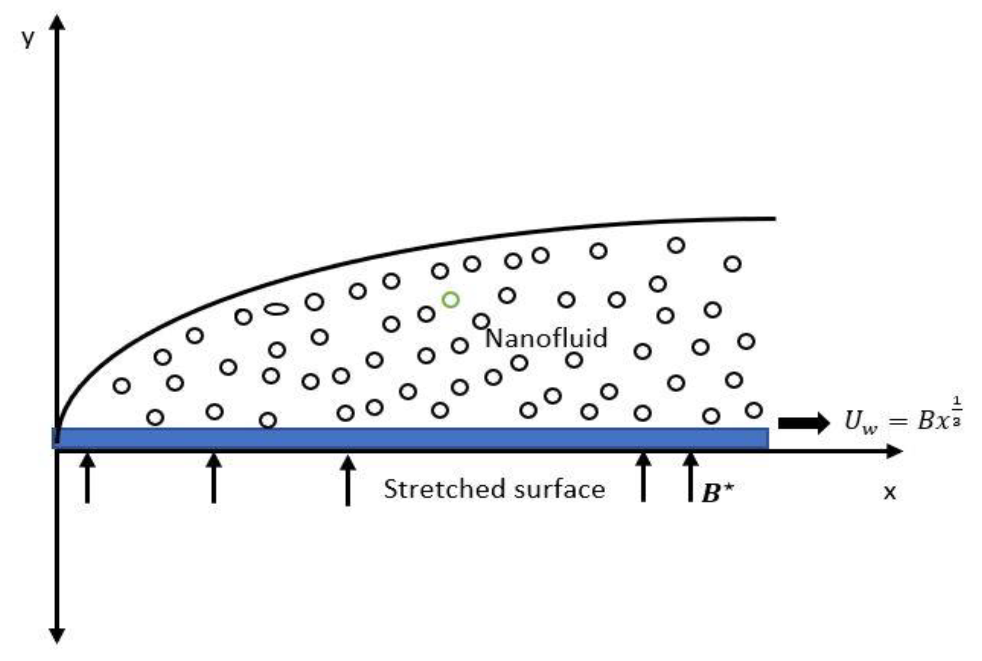
2. Problem Description

We considered the MHD two-dimensional steady boundary layer flow of an incompressible Williamson nanofluid over a non-linear stretching plate. We assumed that the plate is stretching along the $x$-axis, with the varying velocity $u=U_w=B{x}^{\frac{1}{3}}$, and the $y$ direction is taken perpendicular to the $x$ direction, as shown in the Figure 1. The transverse magnetic field $B^{*}=\frac{B_0}{x^{\frac{1}{3}}}$ is exposed in a direction vertical to the flow. It is also supposed that $U_w$, $T_w$, and $C_w$ are the velocity, temperature, and concentration profiles of the fluid at the surface, respectively. Moreover, the ambient temperature and concentration are taken to be $T_{\infty } \mathrm{and} C_{\infty }$, respectively. The continuity, momentum, energy, and concentration equations are taken as specified by Nadeem and Hussain [48,49].

Cauchy stress tensor is defined as

$$\mathit{S}=-p\mathit{I}+\mathbf{\tau },$$

(1)

$$\mathbf{\tau }=\left[ {\mu }_{\infty }+\frac{{\mu }_{o }-{\mu }_{\infty } }{1-\mathsf{\Gamma }\dot{\gamma }}\right]{\mathit{A}}_{1,}$$

(2)

where $\mathit{\tau }$ represents the extra stress tensor, ${\mu }_{\infty }$ and ${\mu }_0$ and are limiting viscosities at infinite and zero shear stress rates, respectively, ${\mathit{A}}_1$ is the first Rivlin Erickson tensor, $\mathsf{\Gamma }>0$ is the time constant, and $\dot{\gamma }$ is denoted as

$$\dot{\gamma }=\sqrt{\frac{1}{2 }}\pi ,$$

(3)

$$\pi =trace{\left({\mathit{A}}_1\right)}^2,$$

We choose the case in which ${\mu }_{\infty }=0$ and $\mathsf{\Gamma }\dot{\gamma }<$ 1. Thus, Equation (2) takes the form

$$\mathit{\tau }=\left[\frac{{\mu }_o}{1-\mathsf{\Gamma }\dot{\gamma }}\right]{\mathit{A}}_1,$$

(4)

Applying Binomial expansion, we obtain

$$\mathit{\tau }={\mu }_o\left[1+\mathsf{\Gamma }\dot{\gamma }\right] {\mathit{A}}_1.$$

(5)

Under given conditions, the boundary layer momentum, energy, and concentration equation with the magnetic field are

$$\frac{\partial u}{\partial x}+\frac{\partial v}{\partial y}=0,$$

(6)

$$u\frac{\partial u}{\partial x}+v\frac{\partial u}{\partial y}=\nu \frac{{\partial }^{2}u}{\partial y^2}+\sqrt{2} \mathsf{\Gamma }\nu \frac{\partial u}{\partial y}\frac{{\partial }^{2}u}{\partial y^2}-\sigma \frac{B^{*2}}{\rho }u,$$

(7)

$$u\frac{\partial T}{\partial x}+v\frac{\partial T}{\partial y}=\alpha \frac{{\partial }^{2}T}{\partial y^2}+\frac{{\rho }_p{c}_p}{\rho c}\left[D_B\frac{\partial C}{\partial y}\frac{\partial T}{\partial y}+\frac{D_T}{T_{\infty }}{\left(\frac{\partial T}{\partial y}\right)}^2\right],$$

(8)

$$u\frac{\partial C}{\partial x}+v\frac{\partial C}{\partial y}=\frac{D_T}{T_{\infty }}\frac{{\partial }^{2}T}{\partial y^2}+D_B\frac{{\partial }^{2}C}{\partial y^2},$$

(9)

The accompanying boundary conditions are

$$\begin{gathered} u=U_w=B{x}^{\frac{1}{3}}, v=0, T=T_w, \\ C=C_w, \mathrm{at} y=0, \\ u\to 0, T\to 0, C\to 0, \mathrm{as} y\to \infty . \end{gathered}$$

(10)

The following transformations are introduced:

$$\begin{gathered} \eta =\frac{1}{x^{\frac{1}{3}} }\sqrt{\frac{B}{\nu }} y, u=B{x}^{\frac{1}{3}}{f}^{\prime }\left(\eta \right), \\ v=-\frac{\sqrt{\nu B}}{3x^{\frac{1}{3}}}\left(2f\left(\eta \right)-\eta f^{\prime }\left(\eta \right)\right), \\ g=\frac{C-C_{\infty }}{C_w-C_{\infty }}, \hspace{1em}\hspace{1em}\theta =\frac{T-T_{\infty }}{T_w-T_{\infty }} . \end{gathered}$$

(11)

Using Equation (11) in Equations (6)–(10), Equation (6) is identically satisfied and Equations (7)–(10) take the following form:

$$\begin{gathered} 3f^{‴}+2f{f}^{″}+\lambda f^{″}{f}^{‴}-M{f}^{\prime }-{f^{\prime }}^2=0, \\ {\theta }^{″}+\frac{2}{3}\mathrm{Pr}f{\theta }^{\prime }+\frac{Nc}{Le}{g}^{\prime }{\theta }^{\prime }+\frac{Nc}{Le\times Nbt}{{\theta }^{\prime }}^2=0, \\ {g}^{″}+\frac{2}{3}Scf{g}^{\prime }+\frac{1}{Nbt}{\theta }^{″}=0, \end{gathered}$$

(12)

$$\begin{gathered} f=0, f^{\prime }=1, \theta =1, g=1, at \eta =0, \\ {f}^{\prime }\to 0, \theta \to 0, g\to 0, as \eta \to \infty . \end{gathered}$$

(13)

where $M=\frac{3\sigma {B_0}^2}{B\rho }$ represents a magnetic parameter, $\lambda =3\mathsf{\Gamma }\sqrt{\frac{2B^3}{v}}$ represents the Williamson parameter, $Nbt=\frac{D_B{T}_{\infty }\left(C_w-C_{\infty }\right)}{D_T\left(T_w-T_{\infty }\right)}$ is the diffusivity parameter, $Sc=\frac{v}{D_B}$ is the Schmidt number, $Pr=\frac{\nu }{\alpha }$ represents the Prandtl number, $Le=\frac{\alpha }{D_B}$ represents the Lewis number, and the heat capacity ratio is represented by $Nc=\frac{{\rho }_p{c}_p}{\rho c}\left(C_w-C_{\infty }\right)$.

The classical boundary layer equation for the viscous flow can be obtained from Equation (12) for $\lambda =M=0$. That is, the fluid behaves as a Newtonian one.

2.1. Friction and Heat Transport Quantities

Some other physical quantities of concern in the current investigation are defined as

$$C_f=\frac{{\tau }_w}{\rho U_w^2}, N{u}_x=\frac{x{q}_n}{T_w-T_{\infty }},S{h}_x=\frac{x{q}_s}{C_w-C_{\infty }}.$$

(14)

where $C_f$ represents the local skin friction, $N{u}_x$ represents the local Nusselt number, and Sh_x represents the local Sherwood number. Shear stress at the wall ${\tau }_w$, wall heat flux $q_n$, and wall mass flux q_s are defined as

$$\begin{gathered} {\tau }_w={\left({\mu }_o\left(\frac{\partial u}{\partial y}+\frac{\mathsf{\Gamma }}{\sqrt{2}}{\left(\frac{\partial u}{\partial y}\right)}^2\right)\right)}_{y=0}, \\ {q}_n=-{\left(\frac{\partial T}{\partial y}\right)}_{y=0}, q_s=-{\left(\frac{\partial C}{\partial y}\right)}_{y=0}. \end{gathered}$$

(15)

By using Equation (11) in Equation (15) and Equation (14), we obtain the dimensionless form

$$\begin{gathered} R{e}_x{c}_f={\left(f^{″}+\frac{\lambda }{6 }{f^{″}}^2\right)}_{\eta =0}, \\ \frac{N{u}_x}{R{e}_x}=-{\theta }^{\prime }\left(0\right), \frac{S{h}_x}{R{e}_x}=-g^{\prime }\left(0\right). \end{gathered}$$

(16)

where $R{e}_x=\sqrt{\frac{x^{\frac{2}{3}}}{B\nu }} U_w$ represents the local Reynolds number.

2.2. Solution Procedure

Non-linear ordinary differential Equation (12) is solved by applying the boundary conditions of Equation (13), in which the velocity profile involves third order, and temperature and concentration profiles are of second order. To solve non-linear ODEs, we use the Shooting method and bvp4c code. Equation (12) is transformed into the system of seven first-order ordinary differential equations. We use the following substitution:

$$f={\mathsf{\zeta }}_1, f^{\prime }={\zeta }_2, f^{″}={\zeta }_3, \theta ={\zeta }_4, {\theta }^{\prime }={\zeta }_5, g={\zeta }_{6 }, g^{\prime }={\zeta }_7.$$

The derived system of simultaneous first-order differential equations is

$$\begin{gathered} {\zeta }_1^{\prime }={\mathsf{\zeta }}_2, {\zeta }_2^{\prime }={\mathsf{\zeta }}_3, {\zeta }_3^{\prime }=\frac{1}{3+\lambda {\zeta }_3}\left({\zeta }_2^2-2{\zeta }_1{\zeta }_3+M{\zeta }_2\right) \\ {\zeta }_4^{\prime }={\zeta }_5, {\zeta }_5^{\prime }=-\frac{2}{3}\mathrm{Pr} {\zeta }_1{\mathsf{\zeta }}_5-\frac{Nc}{Le}{\zeta }_7{\zeta }_5-\frac{Nc}{Le\times Nbt}{{\zeta }_5}^2, \\ {\zeta }_6^{\prime }={\zeta }_7, {{\mathsf{\zeta }}_7}^{\prime }=-\frac{2}{3}Sc {\zeta }_1{\zeta }_7-\frac{1}{Nbt}{\zeta }_5^{\prime }. \end{gathered}$$

(17)

The converted boundary conditions are

$$\begin{gathered} {\zeta }_1\left(0\right)=0, {\zeta }_2\left(0\right)=1, \\ {\zeta }_3\left(0\right)=a, {\zeta }_4\left(0\right)=1, \\ {\zeta }_6\left(0\right)=1, {\zeta }_5\left(0\right)=b, {\zeta }_7\left(0\right)=c. \end{gathered}$$

(18)

To solve the above BVP (Equation (17)) subject to the boundary conditions (Equation (18)), we utilize the shooting technique together with the RK-Fehlberg method. To this end, we guess the three anonymous conditions are ${\zeta }_3\left(0\right)=a$, ${\zeta }_5\left(0\right)=\mathrm{b},$ and ${\zeta }_7\left(0\right)=c$. The reasonable guesses for $a, b,$ and $c$ are chosen such that the corresponding known boundary conditions are almost satisfied for $\eta \to \infty$. Newton’s iterative structure is applied to refine the initial guesses for $a, b,$ and $c$ until the preferred approximation is met. The stopping criteria for the iterative process are

$$\max \left(\left|{\zeta }_2\left({\eta }_{max}\right)-0\right|, \left|{\zeta }_4\left({\eta }_{max}\right)-0\right|, \left|{\zeta }_6\left({\eta }_{max}\right)-0\right|\right)<\mathsf{\epsilon }$$

where $\mathsf{\epsilon }$ is a small positive real number. The computations in the rest of this article are performed with $\mathsf{\epsilon }=$ 10⁻⁶. The effect of various emerging parameters was investigated over an applicable bounded domain $\left[0, {\eta }_{max}\right]$ as a replacement for $\left[0, \infty \right)$. It is observed that for growing values of ${\eta }_{max}$, no substantial variations are detected in the results. In order to test the reliability of the implemented shooting method, the in-house built code was validated with MATLAB built-in bvp4c function.

3. Results and Discussion

The governing non-linear PDE Equations (6)–(9), along with boundary conditions (Equation (10)) of magnetohydrodynamic Williamson nanofluid over a non-linear stretching surface is converted into ODEs by applying the appropriate similarity transformation given by Equation (11). The resulting ODEs are numerically solved by applying the Shooting method and Matlab function bvp4c. The impact of involving parameters such as Magnetic parameter $M,$ Williamson fluid parameter $\lambda$, Diffusivity parameter $Nbt$, Schmidt number $Sc$, Prandtl number $Pr$, Lewis number $Le$, heat capacity ratio $Nc$ on velocity, and temperature and concentration profiles is depicted through graphs and tables. Table 1 illustrates the impact of $\lambda$ and $M$ on the skin friction coefficient. It shows that as we increase the Williamson fluid parameter λ, the value of the skin friction decreases. This is because the higher the Williamson parameter, the smaller the viscosity, which results in a skin friction coefficient reduction. By raising the value of the magnetic field parameter $M$, the value of the skin friction increases. The reason is that the magnetic field reduces fluid velocity, and as a consequence, the value of the skin friction increases.

Table 2 presents the effects of λ, $M$,$Pr$,$Nbt$,$Nc$,$Le,$ and $Sc$ on $-{\theta }^{\prime }\left(0\right)$. By increasing the value of λ, the value for $-{\theta }^{\prime }\left(0\right)$ declines, because the collision of the fluid particle slows down. Moreover, the higher the values of the magnetic field parameter $M$, the lesser is the wall temperature gradient. When we increase $Pr$, which describes correlation between kinematic viscosity and thermal diffusivity, the Nusselt number $-{\theta }^{\prime }\left(0\right)$ increases; that is, the temperature gradient at the surface is increased. By increasing the value of the diffusivity ratio $\left(Nbt\right),$ the value of the $-{\theta }^{\prime }\left(0\right)$ increases because $Nbt$ is the ratio of Brownian diffusivity to thermophoretic diffusivity, and $Nbt$ increases because Brownian diffusivity increases, while it drops down on raising the heat capacities ratio, $Nc.$ The Lewis number $Le$ has an increasing effect on $-{\theta }^{\prime }\left(0\right)$. By augmenting the value of $Le,$ the thermal diffusivity is increased, resulting in growth in $-{\theta }^{\prime }\left(0\right)$.

Table 3 presents the effects of λ, $M$,$Pr$,$Nbt$,$Nc$,$Le,$ and $Sc$ on $-g^{\prime }\left(0\right)$. By enhancing the value of the Williamson fluid parameter $\lambda$, $-g^{\prime }\left(0\right)$ decreases because of a decrease in resistance at the wall. Similar behavior of $-g^{\prime }\left(0\right)$ is noted upon augmenting the values of magnetic parameter $M$ and the Prandtl number $Pr$. With the increase in diffusivity ratio $Nbt$, the Sherwood number, $-g^{\prime }\left(0\right),$ increases. This is because of the greater Brownian motion of fluid particles. When increasing the heat capacities ratio $Nc,$ an increasing trend is seen for $-g^{\prime }\left(0\right)$. Since $Nc$ is the ratio of the heat capacities of nanoparticles to nanofluid, enhancing $Nc$ values mean an increase in nanoparticle heat capacity. It is discerned that the greater the Lewis number $Le,$ the smaller the $-g^{\prime }\left(0\right)$. When increasing the value of the Schmidt number $Sc,$ the value of the $-g^{\prime }\left(0\right)$ also increases. A comparison of Nusselt numbers from the present study and those from Nadeem et al. [48] for different values of Prandtl and Williamson fluid parameters between nonlinear and linear stretching is given in

Table 4. Comparison between linear and nonlinear stretching for $-{\theta }^{\prime }\left(0\right)$ by fixing $Le=4$, M = 0, $N_{bt}=2$, $Nc=0.5$, $Pr=0.5$, and $Sc=0.5$.

$\mathit{\lambda }$	$\mathit{P}\mathit{r}$	Linear Stretching—Nadeem et al. [48]	Nonlinear Stretching—Present Study
0.0		0.314	0.319
0.2		0.309	0.318
0.4		0.302	0.317
	0.2	0.144	0.231
	0.6	0.355	0.347
	1.2	0.588	0.521

. It is readily seen that for both the parameters, the Nusselt number behavior is similar for both linear and nonlinear stretching cases, but its value is higher in the case of nonlinear stretching.

Figure 2 illustrates the impact of λ on f′ (η), θ(η), and $g\left(\eta \right)$. We observe that $f^{\prime } \left(\eta \right)$ decreases as we increase λ. Physically, we can conclude that λ offers more resistance to velocity (see Figure 2a). Increasing of $\lambda$ implies $\mathsf{\Gamma }$ retardation time is higher, which is responsible for the fluid particles regaining their actual position. As a result, the viscosity becomes higher, and the values of temperature and concentration profiles go up. Figure 2b,c describe the influence of the Williamson fluid parameter $\lambda$ on $\theta \left(\eta \right)$ and $g\left(\eta \right)$. By increasing the value of λ, both the temperature and concentration profiles increase because of an increase in the fluid’s resistivity. Figure 3a–c displays the effect of magnetic parameter $M$ on $f^{\prime } \left(\eta \right)$, $\theta \left(\eta \right),$ and $g\left(\eta \right)$. As we increase $M$, the velocity of the fluid decreases, and both temperature and concentration profiles increase. The Lorentz force, which is an opposing force, slows down the motion of fluid, and the velocity boundary layer thickness diminishes. The outcomes of Prandtl $Pr$ on temperature distribution and concentration profile are presented in Figure 4a,b. As we increase the Prandtl number Pr, the temperature profile decreases, and a reduction in the thermal boundary layer is noticed. The increasing of the Prandtl number $Pr$ means making the kinematic viscosity stronger than thermal diffusivity and, as a result, more resistant to fluid flow. The Prandtl number shows the dual behavior on the concentration profile; as we increase the Prandtl number $Pr,$ initially the concentration increases, and at $\eta =2$ it changes its behavior from increasing to decreasing. This is because, far from the surface, viscous forces have negligible effects. Figure 5a,b depicts the effect of the Lewis Number $Le$ on $\theta \left(\eta \right)$ and $g\left(\eta \right).$ As $Le$ is increased, the temperature profile $\theta \left(\eta \right)$ decreases and the thickness of the thermal boundary layer also decreases, and the opposite behavior of the concentration profile $g\left(\eta \right)$ is seen.

For enormous values of $t$, the contribution of last terms of the second and third equations of Equation (12) is negligible; therefore, the concentration profile turns out to be free of temperature. The effect of diffusivity ratio $Nbt$ on both $\theta \left(\eta \right)$ and $g\left(\eta \right)$ is manifested in Figure 6a,b. By increasing $Nbt,$ both $\theta \left(\eta \right)$ and $g\left(\eta \right)$ decrease. The decrease in $g\left(\eta \right)$ is more rapid than $\theta \left(\eta \right),$ and a decrease in thermal boundary layer thickness is also witnessed. The influence of heat capacity ratio $Nc$ on temperature and concentration profiles is shown in Figure 7a,b. The temperature profile $\theta \left(\eta \right)$ increases with an increase in $Nc,$ while a depreciation in the concentration profile $g\left(\eta \right)$ is spotted. The effect of $Sc$ on the concentration is shown in Figure 8. By raising the Schmidt number, the concentration profile is decreased. Since $Sc$ is the ratio of momentum diffusivity and Brownian diffusivity, an increase in Sc results in a decreased Brownian diffusivity, which causes a weaker concentration profile.

4. Conclusions

In this article, we modeled the MHD flow of Williamson nanofluid over a non-linear stretching surface. Similarity transformations were applied, and we obtained a system of non-linear ordinary differential equations. The shooting method was applied to solve them numerically. The combined effects of Williamson parameter $\lambda ,$ magnetic parameter $M$, diffusivity ratio $Nbt$, Prandtl number $Pr$, Lewis number $Le$, Schmidt number $Sc,$ and heat capacities ratio $Nc$ on heat and mass transfer of MHD boundary layer flow of Williamson nanofluid were examined. The salient features of this study are mentioned below:

• The Williamson parameter $\lambda$ and magnetic parameter $M$ have opposite impacts on skin friction coefficient.
• The wall temperature gradient decreases when increasing the value of Williamson parameter λ, $\mathrm{magnetic} \mathrm{parameter}$ $M,$ and heat capacities ratio $Nc,$ whereas it increases for Prandtl number $Pr, \mathrm{diffusivity} \mathrm{ratio} Nbt,$ and Lewis number $Le$. Moreover, the Lewis number $Le$ reveals a strong effect on wall temperature gradient $-{\theta }^{\prime }\left(0\right)$.
• The diffusivity ratio Nbt, heat capacities ratio Nc, and the Schmidt number Sc show direct relation with the Sherwood number −g′(0). An opposite relation is seen with Williamson parameter $\lambda , \mathrm{magnetic} \mathrm{parameter} M, \mathrm{Prandtl} \mathrm{number} Pr,$ and Lewis number $Le$. It is worth mentioning that the most substantial outcome is seen for the Schmidt number $Sc$, where there is a $31\%$ increment in the Sherwood number.
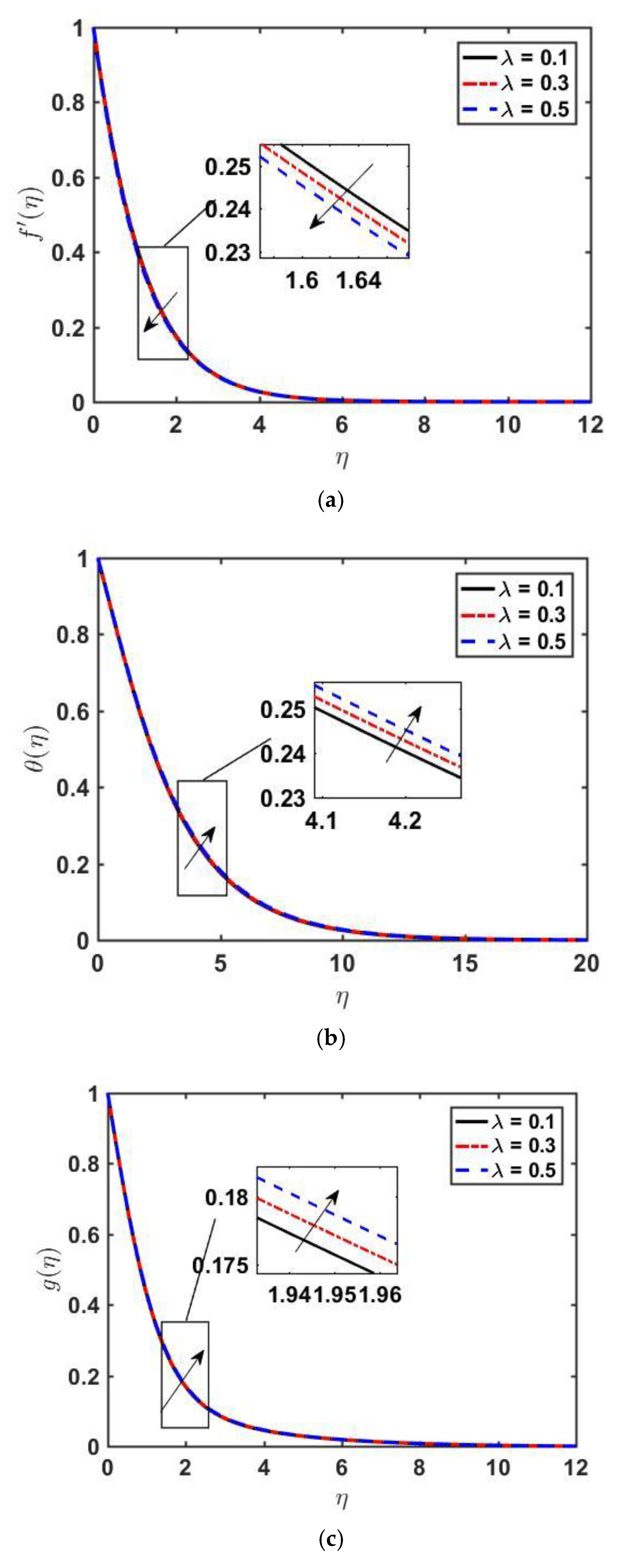
• When raising the values of Williamson parameter $\lambda$ and magnetic parameter $M$, the velocity profile settles at lower values, whereas the temperature and concentration profile settles at higher values. Moreover, the velocity boundary layer contracts, and the thermal boundary layer enlarges.
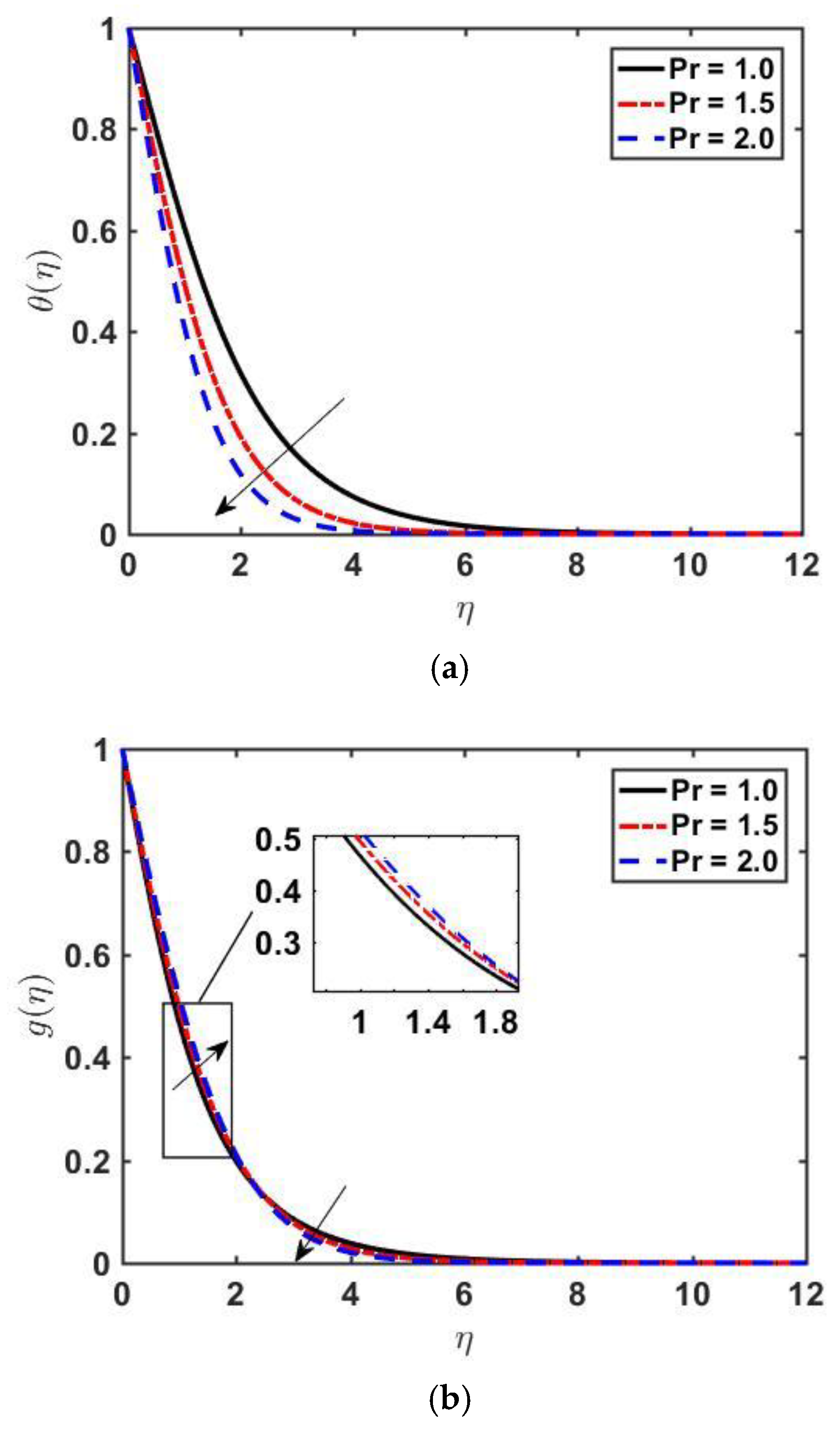
• The temperature profile settles at lower values when raising the Prandtl number $Pr, \mathrm{Lewis} \mathrm{number} Le,$ and diffusivity ratio $Nbt$.
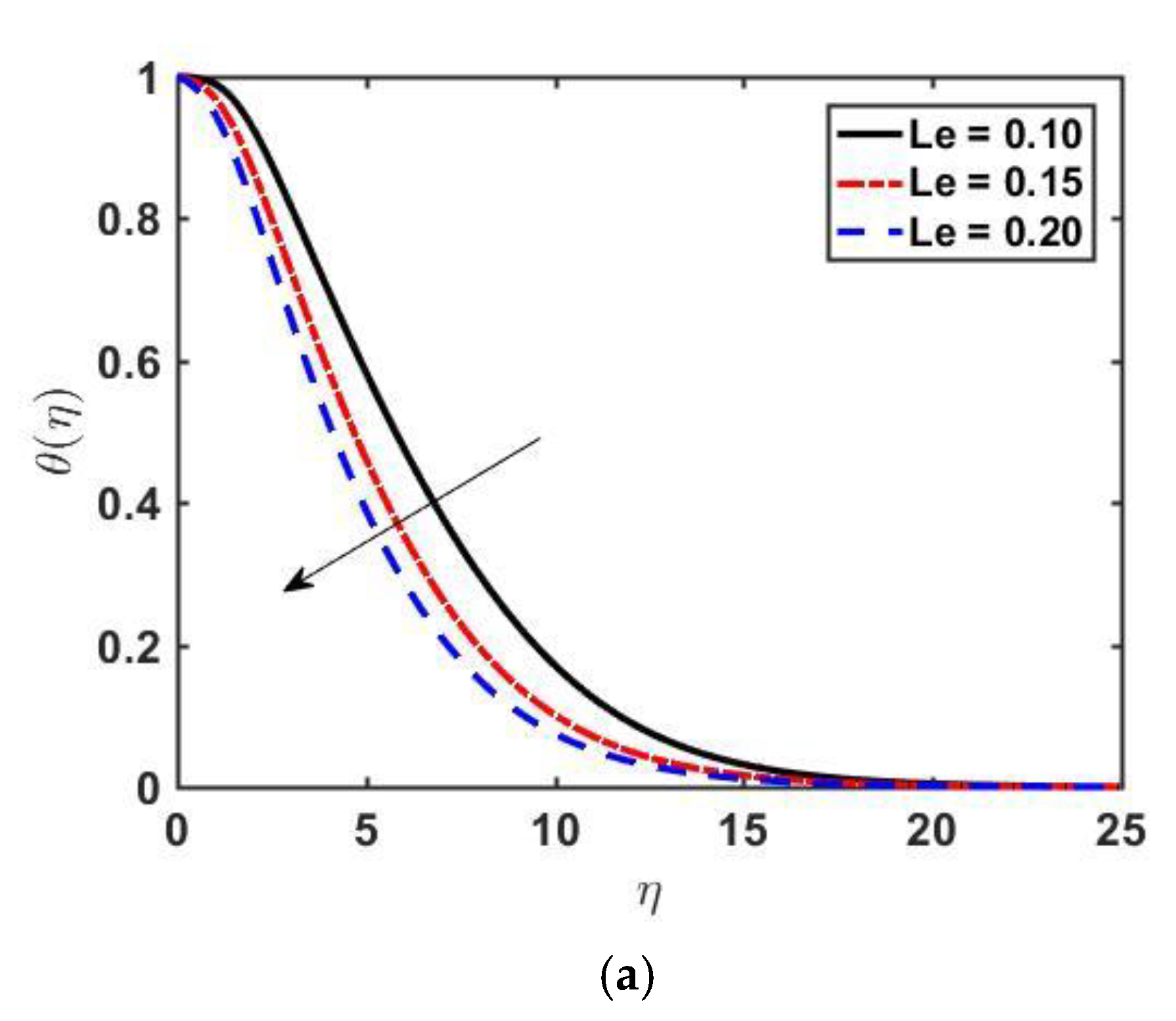
• The concentration profile shows direct relation to the Lewis number $Le$ and an inverse relation to diffusivity $Nbt, \mathrm{heat} \mathrm{capacities} \mathrm{ratio} Nc,$ and Schmidt number $Sc,$ whereas Prandtl number $Pr$ shows dual behavior.

References

1. Williamson, R.V. The flow of pseudoplastic materials. Ind. Eng. Chem. 1929, 21, 1108–1111. [Google Scholar] [CrossRef]
2. Felder, E.; Levrau, C. Analysis of the lubrication by a pseudoplastic fluid: Application to wire drawing. Tribol. Int. 2011, 44, 845–849. [Google Scholar] [CrossRef]
3. Cramer, S.D.; Marchello, J.M. Numerical Evaluation of Models Describing Non-Newtonian Behavior. AIChE J. 1968, 14, 980–983. [Google Scholar] [CrossRef]
4. Lyubimov, D.V.; Perminov, A.V. Motion of a Thin Oblique Layer of a Pseudoplastic Fluid. J. Eng. Phys. Thermophys. 2002, 75, 920–924. [Google Scholar] [CrossRef]
5. Nadeem, S.; Akbar, N.S. Numerical solutions of peristaltic flow of Williamson fluid with radially varying MHD in an endoscope. Int. J. Numer. Methods Fluids 2011, 66, 212–220. [Google Scholar] [CrossRef]
6. Akbar, N.S.; Nadeem, S. Carreau fluid model for blood flow through a tapered artery with a stenosis. Ain. Shams Eng. J. 2014, 5, 1307–1316. [Google Scholar] [CrossRef] [Green Version]
7. Ismail, Z.; Abdullah, I.; Mustapha, N.; Amin, N. A power-law model of blood flow through a tapered overlapping stenosed artery. Appl. Math. Comput. 2008, 195, 669–680. [Google Scholar] [CrossRef] [Green Version]
8. Ahmed, K.; Akbar, T. Numerical investigation of magnetohydrodynamics Williamson nanofluid flow over an exponentially stretching surface. Adv. Mech. Eng. 2021, 13, 168781402110198. [Google Scholar] [CrossRef]
9. Ramzan, M.; Liaquet, A.; Kadry, S.; Yu, S.; Nam, Y.; Lu, D. Impact of second-order slip and double stratification coatings on 3D MHD Williamson Nanofluid flow with cattaneo-christov heat flux. Coatings 2019, 9, 849. [Google Scholar] [CrossRef] [Green Version]
10. Nasrin, R.; Hasanuzzaman, M.; Rahim, N.A. Effect of nano-fluids on heat transfer and cooling system of the photovoltaic/thermal performance. Int. J. Numer. Methods Heat Fluid Flow. 2019, 29, 1920–1946. [Google Scholar] [CrossRef]
11. Vajravelu, K. Viscous flow over a nonlinearly stretching sheet. Appl. Math. Comput. 2001, 124, 281–288. [Google Scholar] [CrossRef]
12. Cortell, R. Viscous flow and heat transfer over a nonlinearly stretching sheet. Appl. Math. Comput. 2007, 184, 864–873. [Google Scholar] [CrossRef]
13. Khan, W.A.; Pop, I. Boundary-layer flow of a nanofluid past a stretching sheet. Int. J. Heat Mass Transf. 2010, 53, 2477–2483. [Google Scholar] [CrossRef]
14. Van Gorder, R.A.; Sweet, E.; Vajravelu, K. Nano boundary layers over stretching surfaces. Commun. Nonlinear Sci. Numer. Simul. 2010, 15, 1494–1500. [Google Scholar] [CrossRef]
15. ASHRAE Handbook—Fundamentals SI Edition Atlanta: American Society of Heating; Refrigerating and Air Conditioning Engineers, Inc.: Boca Raton, FL, USA, 2009.
16. Kole, M.; Dey, T.K. Viscosity of alumina nanoparticles dispersed in car engine coolant. Exp. Therm. Fluid Sci. 2010, 34, 677–683. [Google Scholar] [CrossRef]
17. Dittus, F.W.; Boelter, L.M.K. Heat transfer in automobile radiators of the tubular type. Int. Commun. Heat Mass Transf. 1985, 12, 3–22. [Google Scholar] [CrossRef]
18. Wensel, J.; Wright, B.; Thomas, D.; Douglas, W.; Mannhalter, B.; Cross, W.; Hong, H.; Kellar, J.; Smith, P.; Roy, W. Enhanced thermal conductivity by aggregation in heat transfer nanofluids containing metal oxide nanoparticles and carbon nanotubes. Appl. Phys. Lett. 2008, 92, 9–12. [Google Scholar] [CrossRef]
19. Kulkarni, D.P.; Namburu, P.K.; Ed Bargar, H.; Das, D.K. Convective heat transfer and fluid dynamic characteristics of SiO2—Ethylene glycol/water nanofluid. Heat Transf. Eng. 2008, 29, 1027–1035. [Google Scholar] [CrossRef]
20. Abdul Hamid, K.; Azmi, W.H.; Mamat, R.; Usri, N.A. Heat transfer performance of titanium oxide in ethylene glycol based nanofluids under transition flow. Appl. Mech. Mater. 2014, 660, 684–688. [Google Scholar] [CrossRef]
21. Li, H.; Xiao, H.G.; Yuan, J.; Ou, J.P. Microstructure of cement mortar with nano-particles. Compos. Part B Eng. 2004, 35, 185–189. [Google Scholar] [CrossRef]
22. Vajjha, R.S.; Das, D.K.; Kulkarni, D.P. Development of new correlations for convective heat transfer and friction factor in turbulent regime for nanofluids. Int. J. Heat Mass Transf. 2010, 53, 4607–4618. [Google Scholar] [CrossRef]
23. Berra, M.; Carassiti, F.; Mangialardi, T. Effects of nanosilica addition on workability and compressive strength of Portland cement pastes Constr. Build Mater 2012, 35, 666–675. [Google Scholar] [CrossRef]
24. Syam Sundar, L.; Venkata Ramana, E.; Singh, M.K.; De Sousa, A.C.M. Viscosity of low volume concentrations of magnetic Fe3O4 nanoparticles dispersed in ethylene glycol and water mixture. Chem. Phys. Lett. 2012, 554, 236–242. [Google Scholar] [CrossRef]
25. Azmi, W.H.; Sharma, K.V.; Sarma, P.K.; Mamat, R.; Anuar, S.; Rao, V. Experimental determination of turbulent forced convection heat transfer and friction factor with SiO2 nano-fluid Exp. Therm. Fluid Sci. 2013, 51, 103–111. [Google Scholar] [CrossRef] [Green Version]
26. Azmi, W.H.; Sharma, K.V.; Sarma, P.K.; Mamat, R.; Anuar, S. Comparison of convective heat transfer coefficient and friction factor of TiO2 nanofluid flow in a tube with twisted tape inserts. Int. J. Therm. Sci. 2014, 81, 84–93. [Google Scholar] [CrossRef] [Green Version]
27. Namburu, P.K.; Kulkarni, D.P.; Misra, D.; Das, D.K. Viscosity of copper oxide nanoparticles dispersed in ethylene glycol and water mixture. Exp. Therm. Fluid Sci. 2007, 32, 397–402. [Google Scholar] [CrossRef]
28. Nguyen, C.T.; Desgranges, F.; Roy, G.; Galanis, N.; Maré, T.; Boucher, S.; Angue Mintsa, H. Temperature and particle-size dependent viscosity data for water-based nanofluids—Hysteresis phenomenon. Int. J. Heat Fluid Flow. 2007, 28, 1492–1506. [Google Scholar] [CrossRef]
29. Jang, S.; Choi, S.U.S. Effects of Various Parameters on Nanofluid Thermal Conductivity. J. Heat Transf. 2007, 129, 617–623. [Google Scholar] [CrossRef]
30. Prasher, R.; Bhattacharya, P.; Phelan, P.E. Thermal conductivity of nanoscale colloidal solutions (nanofluids). Phys. Rev. Lett. 2005, 94, 3–6. [Google Scholar] [CrossRef]
31. Awan, A.U.; Abid, S.; Ullah, N.; Nadeem, S. Magnetohydrodynamic oblique stagnation point flow of second grade fluid over an oscillatory stretching surface. Results Phys. 2020, 18, 103233. [Google Scholar] [CrossRef]
32. Abel, M.S.; Mahesha, N. Heat transfer in MHD viscoelastic fluid flow over a stretching sheet with variable thermal conductivity, non-uniform heat source and radiation. Appl. Math. Model. 2008, 32, 1965–1983. [Google Scholar] [CrossRef]
33. Sreedevi, P.; Sudarsana Reddy, P.; Chamkha, A.J. Heat and mass transfer analysis of nanofluid over linear and non-linear stretching surfaces with thermal radiation and chemical reaction. Powder Technol. 2017, 315, 194–204. [Google Scholar] [CrossRef]
34. Jahan, S.; Sakidin, H.; Nazar, R.; Pop, I. Flow and heat transfer past a permeable nonlinearly stretching/shrinking sheet in a nano-fluid: A revised model with stability analysis. J. Mol. Liq. 2017, 233, 211–221. [Google Scholar] [CrossRef]
35. Sakiadis, B.C. Boundary—Layer behavior on continuous solid surfaces: III. The boundary layer on a continuous cylindrical surface. AIChE J. 1961, 7, 467–472. [Google Scholar] [CrossRef]
36. Sakiadis, B.C. Boundary—Layer behavior on continuous solid surfaces: II. The boundary layer on a continuous flat surface. AIChE J. 1961, 7, 221–225. [Google Scholar] [CrossRef]
37. Sakiadis, B.C. Boundary—Layer behavior on continuous solid surfaces: I. Boundary—layer equations for two—dimensional and axisymmetric flow. AIChE J. 1961, 7, 26–28. [Google Scholar] [CrossRef]
38. Crane, L.J. Flow past a stretching plate. Z. Angew. Math. Phys. ZAMP 1970, 21, 645–647. [Google Scholar] [CrossRef]
39. Gupta, P.S.; Gupta, A.S. Heat and Mass Transfer on a Stretching Sheet. Can. J. Chem. Eng. 1977, 55, 744–746. [Google Scholar] [CrossRef]
40. Kameswaran, P.K.; Narayana, M.; Sibanda, P.; Murthy, P.V.S.N. Hydromagnetic nanofluid flow due to a stretching or shrinking sheet with viscous dissipation and chemical reaction effects. Int. J. Heat Mass Transf. 2012, 55, 7587–7595. [Google Scholar] [CrossRef]
41. Khan, U.; Ahmad, S.; Hayyat, A.; Khan, I.; Nisar, K.S.; Baleanu, D. On the Cattaneo-Christov heat flux model and OHAM analysis for three different types of nanofluids. Appl. Sci. 2020, 10, 886. [Google Scholar] [CrossRef] [Green Version]
42. Rashidi, M.M.; Keimanesh, M.; Hung, T.K. Magnetohydrodynamic Biorheological transport phenomena in a porous medium: A simulation of magnetic blood flow control and filtration. Int. J. Numer. Method Biomed. Eng. 2011, 27, 805–821. [Google Scholar] [CrossRef]
43. Oughton, S.; Matthaeus, W.H.; Dmitruk, P. Reduced MHD in Astrophysical Applications: Two-dimensional or Three-dimensional. Astrophys. J. 2017, 839, 2. [Google Scholar] [CrossRef] [Green Version]
44. Carle, F.; Bai, K.; Casara, J.; Vanderlick, K.; Brown, E. Development of magnetic liquid metal suspensions for magnetohydrodynamics. Phys. Rev. Fluids 2017, 2, 1–20. [Google Scholar] [CrossRef]
45. Pedchenko, A.; Gelfgat, Y. Study of the influence of current frequency and non-magnetic gap value on the efficiency of al-alloys stirring in metallurgical furnaces. Magnetohydrodynamics 2007, 43, 363–375. [Google Scholar] [CrossRef]
46. Hainke, M.; Friedrich, J.; Vizman, D.; Müller, G. MHD effects in semiconductor crystal growth and alloy solidification. In Proceedings of the International Scientific Colloquium, Modelling for Electromagnetic Processing, Hannover, Germany, 24–26 March 2003; pp. 73–78. [Google Scholar]
47. Hussain, Z.; Hayat, T.; Alsaedi, A.; Ullah, I. On MHD convective flow of Williamson fluid with homogeneous-heterogeneous reactions: A comparative study of sheet and cylinder. Int. Commun. Heat Mass Transf. 2021, 120, 105060. [Google Scholar] [CrossRef]
48. Nadeem, S.; Hussain, S.T. Flow and heat transfer analysis of williamson nanofluid. Appl. Nanosci. 2014, 4, 1005–1012. [Google Scholar] [CrossRef] [Green Version]
49. Nadeem, S.; Hussain, S.T.; Lee, C. Flow of a williamson fluid over a stretching sheet. Braz. J. Chem. Eng. 2013, 30, 619–625. [Google Scholar] [CrossRef] [Green Version]
Figure 1. Flow geometry of the problem.
Processes 10 01119 g001
Figure 2. Profiles of f ( η ) , θ ( η ) , and g ( η ) versus η for various values of λ by fixing M = 0.5, Pr = 0.5, Le = 3.0, Nbt = 2.0, Nc = 0.5, Sc = 2.0.
Processes 10 01119 g002
Figure 3. Profiles of f′(η), θ ( η ) , and g ( η ) versus η for various values of M , fixing λ = 0.3 ,   P r = 0.5 ,   L e = 3.0 ,   N b t = 2.0 ,   N c = 0.5 , and S c = 2.0 .
Processes 10 01119 g003
Figure 4. Profiles of θ ( η ) and g ( η ) versus η for various values of P r by fixing λ = 0.3 ,   M = 0.5 ,   L e = 3.0 ,   N b t = 2.0 ,   N c = 0.5 , and S c = 2.0 .
Processes 10 01119 g004
Figure 5. Profiles of θ ( η ) and g ( η ) versus η for various values of L e by fixing λ = 0.3 ,   M = 0.5 ,   P r = 0.5 ,   N b t = 2.0 ,   N c = 0.5 , and S c = 2.0 .
Processes 10 01119 g005aProcesses 10 01119 g005b
Figure 6. Profiles of θ ( η ) and g ( η ) versus η for various values of N b t by fixing λ = 0.3 ,   M = 0.5 ,   P r = 0.5 ,   L e = 3.0 ,   N c = 0.5 , and S c = 2.0 .
Processes 10 01119 g006aProcesses 10 01119 g006b
Figure 7. Profiles of θ ( η ) and g ( η ) versus η for various values of N c by fixing λ = 0.3 ,   M = 0.5 ,   P r = 0.5 ,   L e = 3.0 ,   N b t = 2.0 , and S c = 2.0 .
Processes 10 01119 g007
Figure 8. Profile of g ( η ) versus η for various values of S c by fixing λ = 0.3 ,   M = 0.5 ,   P r = 0.5 ,   L e = 3.0 ,   N b t = 2.0 , and N c = 0.5 .
Processes 10 01119 g008