Quality Prediction and Yield Improvement in Process Manufacturing Based on Data Analytics

Abstract

Quality management is important for maximizing yield in continuous-flow manufacturing. However, it is more difficult to manage quality in continuous-flow manufacturing than in discrete manufacturing because partial defects can significantly affect the quality of an entire lot of final product. In this paper, a comprehensive framework that consists of three steps is proposed to predict defects and improve yield by using semi-supervised learning, time-series analysis, and classification model. In Step 1, semi-supervised learning using both labeled and unlabeled data is applied to generate quality values. In addition, feature values are predicted in time-series analysis in Step 2. Finally, in Step 3, we predict quality values based on the data obtained in Step 1 and Step 2 and calculate yield values with the use of the predicted value. Compared to a conventional production plan, the suggested plan increases yield by up to 8.7%. The production plan proposed in this study is expected to contribute to not only the continuous manufacturing process but the discrete manufacturing process. In addition, it can be used in early diagnosis of equipment failure.

1. Introduction

In the manufacturing industry, quality management is a key to competitiveness, productivity, and profit of companies because poor quality management can damage the trust and good image which a company has built up for a long time [1]. For this reason, the importance of quality management in various industries has emerged early on. In early 1950, Juran introduced the idea of Total Quality Control (TQC) to the overall Japanese industry. Lillrank underlined that maintenance is the most important activity in quality management [2]. Bergman and Klefsgo emphasized the role of quality maintenance and repair in production [3]. Especially in continuous-flow process manufacturing, it is very significant to manage quality and defect rate because some defects in a part is directly related to the quality of all subsequent processes.

Recently, with technical advances of the Internet of Things (IoT) technology, the amount of industrial data from sensors is surging and this has promoted the level of automation significantly. From a perspective of quality management, the increasing size of data can be utilized to predict defects so that the quality of final products can be improved. For this reason, there has been a wide range of research on data mining that helps to decide through the modeling of the knowledge extracted from data relations, rules, patterns, and information hidden from the database. In addition, big data analysis, artificial intelligence, machine learning, and deep learning make it possible to conduct quality management more usefully and accurately.

Specifically, this study conducts the data analysis on the continuous manufacturing process with the use of the sensing data of the plastic core extrusion process of a company. Based on the analytic results, yield can be improved by predicting defects in advance and updating production plans. First, for the effective quality management of the continuous manufacturing process, we analyzed the conventional manufacturing process. The problems of it are as follows. Even though well-designed production and quality data are required for better quality management, collecting the data takes a lot of time and cost. For this reason, small and medium-sized enterprises (SMEs) have difficulty for obtaining such data. For example, as shown in Figure 1a, in the extraction process for manufacturing a cylinder product, it is necessary to measure both ends of the product in terms of quality. Therefore, the quality in the middle of the product is not guaranteed.

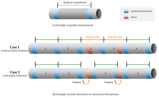
Figure 1. Quality measurement example.

If those defects in the process can be predicted with data analytics preemptively, it enables companies to not only manage a device and product quality but increase a yield. For instance, in Case 1 presented in Figure 1b, if a product is manufactured according to a certain length, two out of five items are defective and therefore a yield is 60%. If the product quality can be predicted before a defect occurs as shown in Case 2, the finished product can be produced after excluding the defective part. Therefore, unlike Case 1 it can be produced the 3rd and 4th finished products and be manufactured 4 items with the same amount of raw materials. Accordingly, the research questions and the corresponding approaches in this study are presented in Table 1.

Table 1. Research Questions and Approaches.

Question	Approach
How will quality data be collected?	Quality data generation through device data through semi-supervised learning.
What techniques will you use to conduct your research?	Using semi-supervised learning, time series prediction, and machine learning.
How do you evaluate performance?	Use evaluation indicators considering characteristics of unbalanced data.

In order to answer all questions, the comprehensive framework with semi-supervised learning, time series prediction, and machine learning is proposed for utilizing unlabeled data in the continuous manufacturing process. For verification of the proposed framework, two experiments were conducted for quality prediction and yield improvement. In the first experiment, after data preprocessing, deep learning and multiple classifiers are applied to predict product quality. In order to handle multiple unlabeled data in continuous flow process manufacturing, the second experiment is designed to predict product quality with the streamline of three models (semi-supervised learning, time series prediction, and multiple classifiers). The detailed procedures are explained in Section 4 and Section 5. Finally, based on the experimental results, an efficient production plan for the plastic extrusion process is derived for improving quality and yield in the continuous-flow process.

2. Related Works & Modeling Techniques

2.1. Data-Driven Quality Management

There have been many studies on data-driven quality prediction and process improvement. Angun researched the neural network-based statistics quality management [3]. Schnell analyzed and improved the production process in the lithium-ion cell manufacturing line by comparing and evaluating the neural network technique and data-mining technique [4]. Ramana predicted quality in the plastic injection molding process as a continuous-flow process by finding data patterns and abnormal symptoms with the use of the data mining technique [5]. With the use of an artificial neural network (ANN) method, Wang predicted the quality of the product in the powder metallurgy compression process which is not a continuous-flow process [6]. Ogorodnyk conducted ANN and decision tree-based classification research in order to predict parts quality in the thermoplastic resin injection molding process [7]. Although many studies have been conducted on the quality prediction of various processes, the quality prediction in process manufacturing has been a little researched. In addition, most studies related to the continuous-flow process focused on the prediction of influential factors on quality. Li studies the ANN model to predict extrusion pressure [8]. Lela researched the linear regression mathematical model for predicting an aluminum molding temperature by using the data recorded continuously in the manufacturing process [9].

2.2. Semi-Supervised Learning

For accurate learning in conventional supervised learning, it is necessary to apply accurate labeling to learning data. A traditional classifier executes learning by using the data with class only. In fact, in the manufacturing process, labeling millions of data costs a lot and requires skillful experts’ long work. However, it is relatively easy to obtain unlabeled data [10]. In the circumstance, it is more important to apply a technology that makes it possible to achieve high performance with the use of a small amount of labeled data. One of the algorithms that can analyze data using a small amount of labeled data is semi-supervised learning (SSL). SSL falls between supervised learning and unsupervised learning. It can be used when data with both input value (X_i) and the target value (y_i), or data with labeled data {(X_i, y_i)} and data with unlabeled data {X_i} are made as a model [11].

Semi-supervised learning can be divided into graph-based and pseudo labeling. In graph-based algorithm, each data sample is expressed as a vertex in a network graph, and links are the measured value of similarity of each vertex [12]. In this algorithm, the label is propagated from the labeled point to the unlabeled point [13]. Typical examples are label propagation (LP) and label spreading (LS). In LP and LS, kernel derivation by the mapping is performed to classify high-dimensional data [14]. The kernels used are the radial basis function (RBF) and k-nearest neighbor (KNN) algorithms, RBF is also called Gaussian kernels. Pseudo-labeling is a model that uses unlabeled data like actual labeled data. Pseudo-labeling produces a pseudo-labeled data by training a classification model with a small amount of labeled data and then predicting the unlabeled data. Then, the pseudo-labeled data and the existing labeled data are trained on the model again to generate a classification model [15].

Today, SSL was applied to a variety of relevant studies, helping to increase research results. Yan utilized SSL in order for the early diagnosis and detection of the air handling unit and showed high accuracy of defect diagnosis [16]. Ellefsen also applied SSL to predict the effective life for engine performance lowering of turbo fan [17]. Sen used SSL to validate data in order to recognize the authenticity of sensor data which is used to judge a defect in the pipe process [18].

2.3. Time-Series Prediction

This study utilizes time-series data which are collected from multiple sensors in a plastic extrusion process of a company. A deep learning technique suitable for time-series analysis is used. Previous studies have used recurrent neural network (RNN), long short-term memory (LSTM) models), and gated recurrent unit (GRU) to predict time-series data. Since the studies using the advantages of RNN are actively conducted, this study applies RNN. Maknickienė utilized RNN as a methodology for predicting the financial market [19]. Zhu used RNN to analyze the components and structural change of soil [20]. In addition, defects in electrochemical sensors or polymer were diagnosed using machine learning models such as RNN, LSTM, and CNN [21,22]. Aside from that, RNN is applied to the prediction for temperature control of the variable frequency based oil cooler in the industrial process. As such, RNN is used to predict a time-series process [23].

2.4. RNN

RNN is a type of ANN. As one of the deep learning techniques, it recirculates the output of a hidden layer as an input to learn sequential (time-series) data for prediction or classification. RNN is an extension of the existing feed-forward neural network using a loop that iterates the previous input into the output. RNN has the iterative state in which the activation in each step relies on the activation in its previous step, in order to process sequential data input. When the sequence data $\mathrm{x}=\left(x_1,x_2,x_3,\cdots ,x_t\right)$ (x_t is ith time data) is given, RNN updates hidden state h_t repeatedly, where ∅ is a nonlinear function like logistic sigmoid function or tangent function [12]:

$$h_t=\{\begin{array}{cc}0& ift=0\\ \varnothing (h_{t-1},x_{t,}& otherwise\end{array}$$

(1)

2.5. Classification

Machine learning is a method inferring a system function based on a pair of data and labels. An inference process is dependent on input features. If the prediction result of new input data is a continuous value, it is used for regression analysis; if a discrete value, it is used for classification [24]. This study uses logistic regression, decision tree, random forest, linear discriminant analysis (LDA), Gaussian naive Bayes (GNB), K-nearest Neighbor (KNN), and support vector classifier (SVC) among machine learning classification techniques, and ANN as a deep learning technique.

2.6. Differences from Previous Studies

Although many studies have performed quality prediction and used SSL or RNN, some features can be found when classifying related studies by process. First, in studies on quality prediction, research on discrete processes is more abundant than research on continuous processes. In addition, most studies related to the quality of the continuous process predicted the factors of facilities that affect the quality overall, not the quality of the products themselves. Second, studies using SSL have been applied to prediction in various fields, but most of them have been used to generate data in image processing. Studies related to manufacturing processes mainly focused on defect detection and monitoring systems and did not consider quality prediction. In addition, in the studies using RNN, although various predictions were made for time series data, the number of papers predicting the quality in a continuous process was very small. Therefore, this study proceeds with the prediction of the quality of the continuous process, which was not done well in the previous study. Quality prediction is carried out by collecting equipment data. In the previous study, sensor data is used to predict and maintain the quality of the process, and there are studies using deep learning and machine learning for sensor-based prediction [21,22]. For improving the quality prediction of small data, we apply SSL to labeling and RNN to generating predictive feature data. Finally, we classify the data, which are SSL and RNN applied, through classification techniques for quality prediction. It is intended to efficiently operate the production in a continuous process and use the quality prediction results to check how much the yield can be finally improved.

3. Data Introduction and Statistical Analysis

This study collected the data in a plastic extrusion process as a continuous-flow manufacturing process. In the plastic extrusion process, 20,801 instances were collected from each device sensor at an interval of one second. Among attributes in the dataset, we considered 26 attributes such as extrusion temperature, screw speed, external temperature, external humidity, and water temperature because some attributes have the same values during the collection period. Table 2 summarizes the attributes used in this study.

Table 2. Attributes description.

Attribute	Description	Type
TIEXT1	Extrusion temperature 1	continuous
TIEXT2	Extrusion temperature 2	continuous
TIEXT3	Extrusion temperature 3	continuous
TI_DIES1	Dies temperature 1	discrete
TI_DIES2	Dies temperature 2	discrete
TI_DIES3	Dies temperature 3	discrete
TI_DIES4	Dies temperature 4	discrete
TI_DIES5	Dies temperature 5	0
RPM1_SCREW	Screw velocity	discrete
RPM2_EXT	Extrusion velocity	discrete
TI_CYL1	Cylinder temperature 1	discrete
TI_CYL2	Cylinder temperature 2	discrete
TI_CYL3	Cylinder temperature 3	discrete
TI_CYL4	Cylinder temperature 4	discrete
TI_CYL5	Cylinder temperature 5	discrete
TI_CYL6	Cylinder temperature 6	discrete
Outtemp1	External temperature 1	continuous
Outtemp2	External temperature 2	continuous
Outtemp3	External temperature 3	continuous
Outwet1	External humidity 1	continuous
Outwet2	External humidity 2	continuous
Outwet3	External humidity 3	continuous
Water_1	Water temperature 1	continuous
Water_2	Water temperature 2	continuous
Water_3	Water temperature 3	continuous
Water_4	Water temperature 4	continuous

If a final product exceeds a given tolerance, the product is marked as defective. Based on the product specification with an inner diameter of 6 inches and a thickness of 8 cm, the allowable error of process is determined as ±0.2 mm in thickness and ±0.5 mm in thickness. For the application of a classifier, the quality value for products was coded as a binary value (1 for defective and 0 for acceptable). In this study, 3839 defective products (about 18%) of 20,801 data were used. Note that quality value means not the quality of a single piece of product, but the quality of a part of a product manufactured every second.

To find the characteristics of each data, we conducted a statistical analysis of the line graph and box plot. Figure 2 illustrates the line graphs of the features of continuous data. TIEXT1~3 and Water_1~4 followed a similar trend by the sensor. Nevertheless, a temperature was changed depending on a sensor position so that it went up or down overall. However, Outtemp and Outwet are changing irregularly. Through this, it can be seen that TIEXT and Water are control variables and Outtemp and Outwet are measurement variables.

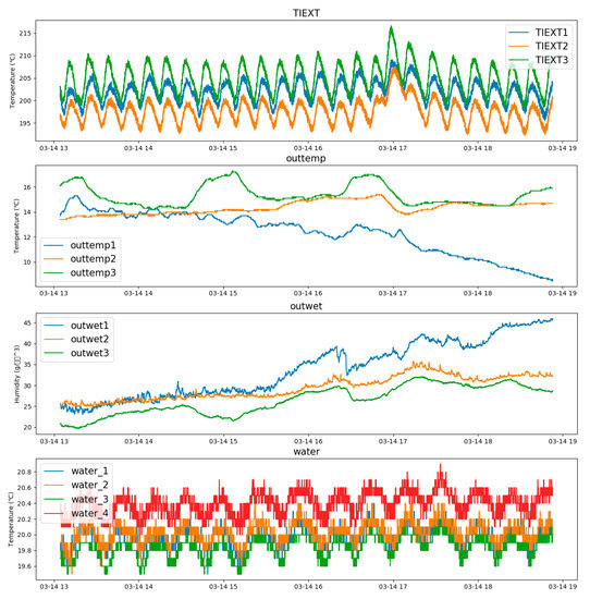
Figure 2. Extrusion temperature, external temperature, external humidity, water temperature graph.

In outliner analysis, features of continuous data were checked with the use of the box plot. Box plot is one of the various statistical techniques named exploratory data analysis. It is used to visually identify a pattern that can be hidden in a data set. Figure 3 represents the illustrative box plots of continuous data. The darker the point representing an outlier is, the more outliers are distributed in a relevant range. According to the analysis, Outtemp and Outwet had no outliers, and TIEXT2~3 and Water_1~4 had sixty outliers of each one of 329, 5, 315, 237, and 3174. Although there were a significant number of outliers, these outliers were concentrated in a few particular sections. Taking this into consideration, this study did not regard the outliers as outliers caused by data errors.

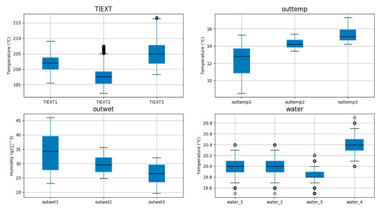
Figure 3. Illustrative box plots of continuous data.

The distribution of discrete data is shown in Table 3. In the case of dice temperature and cylinder temperature, sensors are located differently so that data values and sections are different. The number of data related to the speed of RPM1_SCREW and RPM2_EXT is small.

Table 3. Data sets of discrete data.

Attribute	Data Set
TI_DIES1	{190, 191, 192, 193, 194, 195, 196, 197, 198, 199, 200}
TI_DIES2	{191, 192, 193, 194, 195, 196, 197, 198, 199, 200, 201, 202}
TI_DIES3	{192, 193, 194, 195, 196, 197, 198, 199, 200, 201, 202, 203, 204}
TI_DIES4	{198, 199, 200, 201, 202, 203, 204, 205, 206, 207, 208, 209, 210, 211}
RPM1_SCREW	{24, 25}
RPM2_EXT	{1202, 1203, 1204}
TI_CYL1	{171, 172, 173, 174, 175, 176}
TI_CYL2	{180, 181, 182, 183, 184, 185, 186, 187, 188, 190}
TI_CYL3	{184, 185, 186, 187, 188, 190, 191, 192, 193}
TI_CYL4	{190, 191, 192, 193, 194, 195, 196, 197, 198}
TI_CYL5	{192, 193, 194, 195, 196, 197, 198}
TI_CYL6	{194, 195, 196, 197, 198, 199}

The results from the correlation analysis on features are shown in Figure 4. Pearson correlation coefficient was applied, in which a correlation coefficient is a value between–1 and +1. The closer the coefficient is to ±1, the more there is a correlation. A correlation coefficient was presented with different color temperature. The larger a correlation coefficient is, the darker the color temperatures are. According to the analysis, the correlation coefficients of the sensors in close proximity, such as extrusion temperatures (TIEXT1~3) and dice temperatures (TI_DIES2~3), were mostly high. Aside from that, the correlation coefficients between TIEXT, TI_DIES4, Outwet, and Outtemp1 were high.

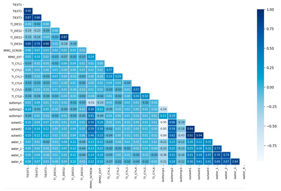
Figure 4. Schematic of the correlation coefficient between features.

Additionally, the correlation coefficients between quality values and features were analyzed. In Table 4, the analysis results are presented in descending sort order after taking absolute values. Given that all of the correlation coefficients between quality values and features are small, a particular feature does not determine a quality value.

Table 4. Correlation coefficients between quality values and features.

Attribute	Correlation	Attribute	Correlation
TI_DIES1	0.2658	Outtemp1	0.0037
TI_CYL5	0.2278	Outwet3	0.0037
TI_CYL4	0.1411	TI_CYL2	0.0036
TI_CYL6	0.1034	TIEXT3	0.0033
Water_3	0.0461	Outwet2	0.0027
Water_4	0.0417	TI_DIES4	0.0015
Water_2	0.0341	Outwet1	0.0014
Water_1	0.0284	TI_DIES3	0.0012
Outtemp3	0.0257	TI_DIES2	0.0009
RPM1_SCREW	0.0192	RPM2_EXT	0.0009
TI_CYL3	0.0163	TIEXT2	0.0002
TI_CYL1	0.0075	TIEXT1	0.0001
Outtemp2	0.0075

4. Quality Prediction in Process Manufacturing

In this chapter is described the first experiment for predicting product quality with the uses of machine learning classification models. In all the analyses, Python 3.6.10 was applied and the software libraries used are listed in Table 5.

Table 5. List of used libraries for python programming.

Library	Version	Purpose
Numpy	1.18.1	fundamental package for scientific computing
pandas	1.0.1	data analysis and manipulation tool
Keras	2.3.1	deep-learning API
scikit-leam	0.22.1	tools for predictive data analysis

4.1. Data Preprocessing

For the machine learning based quality prediction, this study applied ANN, Logistic Regression, Decision Tree, Random Forest, LDA, Gaussian NB, KNN, and SVC. In consideration of the imbalanced data (with different class ratio) used in this study, learning data sets were preprocessed before a classification model was created. For preprocessing, resampling and feature scaling were used. As resampling techniques for adjusting imbalanced data, there are undersampling, oversampling, and hybrid methods [25], each of which is described in Table 6.

Table 6. Three resampling techniques.

Methods	Description
Undersampling	Reduces the imbalance rate by randomly removing some elements of the majority class from the data set.
Oversampling	It takes the opposite approach to Undersampling. Instead of reducing the majority class, add the minority class to the training set as a cloned or disturbed variant.
Hybrid method	Combine Undersampling and Oversampling in a data balancing approach.

Of 20,801 original data, 18,218 are non-defective product data, and 2583 are defective product data. In this study, the set ratio of training data to test data is 5 to 5. Of 10,401 training data, 9131 are non-defective product data (about 88%), and 1270 are defective product data (about 12%). Since there was a large difference between the majority class and minority class, Oversampling was applied to set the class ratio. After resampling, 9131 defective product data and 9131 non-defective product data were created equally. In addition, since feature values vary and each data scale is irrelevant, feature scaling is applied to unify a range of features. Feature scaling is used to compare and analyze multi-dimensional values easily, and to improve the stability and convergence speed in the optimization process [26]. As described in Section 4.1, features had some data including outlier. In consideration of the point, RobustScaler of the Python scikit-learn library was used as a preprocessing method. RobustScaler is the technique of removing a median value, scaling data in the range of IQR (Inter-quartile range), and therefore minimizing the influence of outliers. The processing method of RubustScaler ensure that each feature has a median of 0 and a quartile of 1 so that all features are on the same magnitude [27].

4.2. Results of Quality Prediction through the Classifier

Cross-validation was applied to select a model fitting process data. Cross-validation can prevent overfitting and data sampling bias and can be applied if there are a small number of data records, and can be used to check the generality of a model [28]. K-fold cross-validation was applied. The technique splits the total data into k sets, selects each set as a test set at a time, and executes cross-validation a total of k times. At this time, k-1 data sets except for the data selected as a test set are used as a training set [29]. Performance indices for model evaluation generally use the confusion matrix as shown in Table 7. Among the indices, balanced accuracy is applied. General accuracy does not support a significant confidence interval and especially does not provide the safety device for biased data like imbalanced data. Therefore, to overcome the problem, balanced accuracy is replaced [30]. Balanced accuracy is applied to the binary and multiple class classification for processing imbalanced data sets and is defined as the mean of the recalls obtained from classes:

$$\begin{array}{c}\hfill \mathrm{accuracy}=\frac{predicted positive}{total predicted}=\frac{TP}{TP+TN}\hfill \\ \hfill \mathrm{balanced}\mathrm{accuracy}=\frac{sensitivity+specificity}{2}=\left(\frac{TP}{TP+FN}+\frac{TN}{FP+TN}\right)/2\hfill \end{array}$$

Table 7. Confusion matrix.

	Actual Positive	Actual Negative
Predicted positive	TP	FP
Predicted negative	FN	TN

Of the applied classifiers, ANN was designed to be a model with two hidden layers, each of which has 100 neurons and 80 neurons, respectively. Rectified linear unit (ReLU) and sigmoid were used as activation functions, and Adam was used as an optimizer. ReLU is the most frequently applied activation function. A final classification result should be a binary number: either non-defective product (0) or defective product (1). Therefore, sigmoid was applied to an output layer. The count of repetition was set to 1000, and the batch size was set to 10. For model learning, validation data was set to 30%, and then early stopping was applied. Early stopping can prevent underfitting and overfitting. It can stop learning even if the repetition count has yet to be reached, only if the repetition count, in which no more performance is improved, exceeds a particular count. In this study, the count was set to ‘5′. The results of cross-validation (k = 5) are presented in Table 8.

Table 8. Results of cross-validation applied with simple classification.

Models	Balanced Accuracy
ANN	0.68 (±0.05)
Logistic Regression	0.70 (±0.02)
Decision Tree	0.79 (±0.10)
Random Forest	0.65 (±0.22)
LDA	0.71 (±0.01)
GNB	0.68 (±0.08)
KNN	0.52 (±0.07)
SVC	0.61 (±0.03)

It was found that a model has more generality in the order of decision tree, LDA, and logistic regression. For the evaluation of the performance of the classification model, log loss, and receiver operating characteristic (ROC) curves were analyzed as well as the performance found in cross-validation. The two performance indexes can be checked after data fitting in the model so that they are not used in cross-validation. Log loss is called cross-entropy and can be compared with accuracy. Accuracy means that a prediction value is equal to an actual value. Log loss takes into account uncertainty depending on how different the label is based on probability. Therefore, with log loss, it is possible to obtain a delicate view of the model performance. The lower a log loss is, the better value is. In the ROC curve, false positive rate (FPR) is displayed on the x-axis and true positive rate (TPR) on the y-axis. At this time, FPR is a rate of negative cases wrongly classified as positive ones, and TPR is a rate of positive cases that have labels specified correctly [31]. ROC can calculate the area under the curve (AUC) and provides the score that can be used to compare the AUC model. Generally, a ROC curve is effective at severe class imbalance when minority class has a small number of data [32]. An unskilled classifier scores 0.5, whereas a perfect classifier scores 1.0. The classification results after the consideration of the added performance evaluation measures are presented in Table 9.

Table 9. Results of actual classification prediction with performance evaluation measures.

Models	Balanced Accuracy	Log Loss	AUC (ROC Curve)
ANN	0.4998	4.37048	0.5329
Logistic Regression	0.6747	10.6076	0.7468
Decision Tree	0.8710	2.16202	0.8710
Random Forest	0.5372	4.04170	0.9184
LDA	0.6745	11.07588	0.7484
GNB	0.6430	8.74776	0.7304
KNN	0.5048	7.06060	0.5099
SVC	0.5021	4.41034	0.5883

According to the final classification performance analysis, the best model in terms of balanced accuracy and log loss was decision tree, and the best model in terms of the ROC curve was random forest. We compared two models concerning the confusion matrix as shown in Table 10. In the case of random forest, FP (the case that was predicted to be defective though non-defective) was very low, but FN (the case that was predicted to non-defective though defective actually) was high. In the case of the decision tree, each error was distributed in a balanced way. In terms of the number of incorrectly classified items, decision tree 365 + 286 = 651, and random forest 2 + 1215 = 1217. Given that, we may conclude that decision tree has better performance.

Table 10. Confusion matrices applied with simple classification.

Models	Confusion Matrix
		Predicted as Good	Predicted as Bad
Decision Tree	Actual good	8722	365
	Actual bad	286	1027
Random Forest	Actual good	9085	2
	Actual bad	1215	98

4.3. Simple Classification Feature Importance

Feature Importance was analyzed in order to find which features were considered to be critical factors in data classification by decision tree as shown in Figure 5. In terms of feature importance, the top five features of all were TI_CYL5, TI_DIES1, and TIEXT1~3, each of which scored 0.1896, 0.1757, 0.1101, 0.1085, and 0.1046. The top five of 25 features accounted for 69% influence.

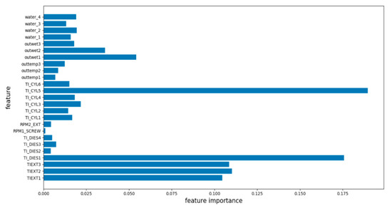
Figure 5. Feature importance in case of Decision Tree.

5. Yield Improvement Method

Labeled data requires expensive labor and a lot of time so that it is hard to collect plenty of labeled data. On the contrary, it is far easy to obtain a lot of unlabeled data. For example, in text classification, it is possible to access a large document database easily through web crawling, and some of the collected data is classified manually [33]. In the second experiment, on the assumption that there are numerous unlabeled data in the product manufacturing process, the quality of the continuous-flow process is predicted with the use of SSL and time-series prediction.

5.1. Research Framework

The framework in the second experiment is illustrated in Figure 6. The whole process is divided into Step 1, Step 2, and Step 3. In Step 1, on the assumption that unlabeled data and labeled data coexist, unlabeled data is labeled through SSL. In Step 2, the future value of feature data is generated through time-series prediction. In Step 3, quality is finally predicted and classified on the basis of the labeled data created in Step 1 and the data created through time-series prediction in Step 2.

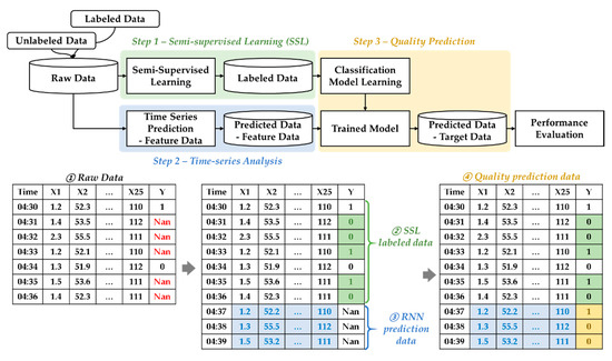
Figure 6. Research framework and some illustrative data.

5.2. STEP1—Semi-Supervised Learning

When a small amount of data is resampled or scaled, bias can occur. Therefore, the data is analyzed without data preprocessing. The ratio of training data to test data was set to 5:5. SSL was conducted only with the use of 10,400 training data. Of the training data, 6281 (about 60%) were randomly deleted, and 40% (4119 data) was used to label the deleted data. The SSL method applied pseudo labeling and graph-based classifier. Pseudo labeling applied seven classifiers except for ANN among the classifiers used in Section 4.2. Label spreading and label propagation as graph-based SSL classifiers applied radial basis function (RBF) and KNN kernels, respectively. Accordingly, SSL was applied to a total of eleven cases, and cross-validation (k = 5) was conducted. Table 11 presents the results. Given the results of cross-validation, decision tree and random forest had the most generality of the model.

Table 11. Results of cross-validation applied with semi-supervised learning (k = 5).

Classifiers	Models	Balanced Accuracy
Pseudo Labeler	Logistic Regression	0.52 (±0.03)
	Decision Tree	0.87 (±0.08)
	Random Forest	0.64 (±0.20)
	LDA	0.53 (±0.03)
	GNB	0.55 (±0.09)
	KNN	0.57 (±0.08)
	SVC	0.50 (±0.00)
Label Spreading	RBF	0.54 (±0.07)
	KNN	0.56 (±0.05)
Label Propagation	RBF	0.54 (±0.07)
	KNN	0.56 (±0.04)

The results from the application to a real model are shown in Table 12. In this case, SVC classifies all values as the non-defective product so that it is meaningless in comparison to different performance evaluation measures. For this reason, it was excluded. For the comparison of model performance, balanced accuracy, log loss, and AUC of the ROC curve were used. In respect of balanced accuracy and log loss, the top five models were equal. In terms of the ROC curve, decision tree and random forest were excellent. Confusion matrices were analyzed in order to select a final model. As a result, random forest was found to have good performance as shown in Table 13. On balance, labeled data through random forest-based pseudo labeler are trained in the final classification process of Step 3, therefore, quality is predicted.

Table 12. Results of actual SSL prediction with performance evaluation measures.

Classifiers	Models	Balanced Accuracy	LOG LOSS	AUC (ROC Curve)
Pseudo Labeler	Logistic Regression	0.5541	3.9317	0.7483
	Decision Tree	0.9273	1.1493	0.8075
	Random Forest	0.9198	0.8248	0.9197
	LDA	0.575	3.9922	0.7400
	GNB	0.6170	4.4707	0.7433
	KNN	0.8070	2.2326	0.5043
Label Spreading	RBF	0.8835	1.7212	0.5747
	KNN	0.7187	3.2554	0.5540
Label Propagation	RBF	0.8833	1.7377	0.5461
	KNN	0.7065	2.9859	0.5161

Table 13. Confusion matrices applied with semi-supervised learning (k = 5).

Classifiers	Models	Confusion Matrix
			Predicted as Good	Predicted as Bad
Pseudo Labeler	Decision Tree	Actual good	5375	109
		Actual bad	100	697
	Random Forest	Actual good	5458	26
		Actual bad	124	673
	KNN	Actual good	5376	108
		Actual bad	289	508
Label Spreading	LS—RBF	Actual good	5335	149
		Actual bad	164	633
Label Propagation	LP—RBF	Actual good	5332	152
		Actual bad	164	633

5.3. STEP2—RNN Time Series Analysis

In Step 2, a test data set is predicted with the use of the training data set of features. For time-series prediction, the RNN model was applied, and a model with two hidden layers was designed. One hidden layer has 500 neurons, and the other has 1000 neurons. As an activation function, ReLU was used. Adam was used as an optimizer. Individual learning was conducted for each feature. The count of repetition was set to 1000, and the batch size was set to 10. For model learning, validation data was set to 30%, and then early stopping was applied. Early stopping can prevent underfitting and overfitting. It can stop learning even if the repetition count has yet to be reached, only if the repetition count, in which no more performance is improved, exceeds a particular count. In this study, the count was set to ‘5′. For the features expressed as discrete data in Table 2, the output value was rounded off and then changed to an integer number. In comparison between a predicted value and a real value, the performance was evaluated with mean absolute percentage error (MAPE). MAPE is a measure of prediction accuracy of a forecasting method in statistics. It usually expresses the accuracy as a ratio defined in Equation (2). A is the actual value and F is the predicted value. Smaller MAPE means better predicted performance. The mean, standard deviation, minimum value, and maximum value of MAPEs of all features are 0.2530, 0.5239, 0, and 2.1950, respectively. More details are shown in Table 14:

$$\mathrm{MAPE}=\left(\frac{1}{n}{\displaystyle \sum }_{t=1}^n\left|\frac{A_t-F_t}{A_t}\right|\right)\ast 100$$

(2)

Table 14. RNN Prediction performance.

Feature	MAE	RMSE	MAPE
TIEXT1	0.3017	0.3822	0.1488
TIEXT2	0.4023	0.6302	0.2010
TIEXT3	0.2991	0.3797	0.1459
TI_DIES1	0.0324	0.1801	0.0166
TI_DIES2	0.0246	0.1569	0.0125
TI_DIES3	0.0365	0.1909	0.0182
TI_DIES4	0.0246	0.1569	0.0121
RPM1_SCREW	0.0000	0.0000	0.0000
RPM2_EXT	0.1465	0.3828	0.0122
TI_CYL1	0.0451	0.2124	0.0259
TI_CYL2	0.0533	0.2309	0.0287
TI_CYL3	0.0700	0.2646	0.0371
TI_CYL4	0.0679	0.2606	0.0350
TI_CYL5	0.0771	0.2776	0.0394
TI_CYL6	0.0523	0.2288	0.0266
Outtemp1	0.0178	0.0294	0.1740
Outtemp2	0.0566	0.0708	0.3793
Outtemp3	0.0328	0.0389	0.2129
Outwet1	0.6812	0.7103	1.6803
Outwet2	0.1353	0.1770	0.4122
Outwet3	0.6642	0.7560	2.1950
Water_1	0.0238	0.0378	0.1186
Water_2	0.0262	0.0384	0.1308
Water_3	0.0275	0.0393	0.1379
Water_4	0.0253	0.0413	0.1239

5.4. STEP3—Classification

In Step 3, the final classification data is obtained for yield improvement. In Step 1, loss data were generated by random forest-based pseudo labeler. In Step 2, feature data were predicted with RNN. In the last step, classification is performed on the basis of the data generated in each previous step, and a future quality value is finally predicted. The classifiers used in Section 4.2 were also applied in this step. Table 15 and Table 16 present the final classification performance and results after random forest (SSL) was applied. As shown in Table 15, decision tree and random forest had excellent performance in terms of all performance indexes. The final objective of this study is to increase the yield through quality prediction. For the reason, based on the quality value predicted in Step 3, how much more the process method can increase a yield than a conventional process method will be calculated.

Table 15. Results of classification applied after semi-supervised learning (Random Forest).

Models	Balance Accuracy	Log Loss	AUC (ROC Curve)
ANN	0.5000	4.3626	0.7360
Logistic Regression	0.5784	4.5886	0.7521
Decision Tree	0.8434	2.1764	0.8791
Random Forest	0.7099	2.9206	0.9252
LDA	0.5417	4.4191	0.7393
GNB	0.5102	4.2995	0.7272
KNN	0.5045	6.6088	0.5059
SVC	0.5000	4.3626	0.4475

Table 16. Confusion matrices of classification applied after semi-supervised learning (random forest).

Models	Confusion Matrix
		Predicted as Good	Predicted as Bad
Decision Tree	Actual good	8797	285
	Actual bad	370	943
Random Forest	Actual good	8947	135
	Actual bad	696	671

5.5. Yield Improvement Results

Yield is calculated as ‘the number of non-defective products (a) divided by total output (A)’. Typically, products are manufactured in the equidistant interval method in which products are cut at a given interval according to continuous production. In this case, if any part of a product is defective, the product is judged to be a defective product. Therefore, this study proposes a new production method that predicts quality through SSL, time-series prediction, and classifier and performs product cutting in consideration of the part predicted to be defective. In the proposed new method, the value calculated with the formula ‘the number of non-defective products (b, c, d)/total output (A)’ is measured as a yield for comparison. Total output is the value calculated in the conventional equidistant interval production method. Two models of decision tree and random forest were used for the final classification.

(1)

If the predicated quality of all items is a non-defective product in a production length during a unit time, the products are manufactured.

(2)

If the manufactured products include any defective product, they are regarded as defective products.

Without the application of SSL and RNN, a small amount of data was applied to quality prediction. Of all the data (10,401 data), 60% were deleted randomly, and 40% (4120 data) were trained with Decision Tree, which showed the best performance in Section 4.2. Based on these small numbers of data, 10,395 data were predicted again. In addition, the quality of the Step 3 results was predicted with 40% of the data, and the results are shown in Section 5.4. Confusion matrix, which is the result of each prediction, is shown in Table 17.

Table 17. Final result comparison through confusion matrix.

Pre-Processing	Models	Confusion Matrix
			Predicted as Good	Predicted as Bad
Semi-Supervised Learning	Decision Tree	Actual good	8797	285
		Actual bad	370	943
	Random Forest	Actual good	8947	135
		Actual bad	696	671
Simple Classification	Decision Tree	Actual good	8437	650
		Actual bad	260	1053

Table 18 presents the numbers of the products generated according to the prediction results and the proposed method. Given the final number of non-defective products, there was no yield improvement effect even if product cutting was executed in consideration of defect occurrence. However, as shown in the study results, the proposed method increased to yield more than a conventional production method when a production unit time was larger than six seconds (c, d). In the case of decision tree, a yield increased in all the unit time slots after six seconds and went up by a maximum of about 8.70% (c). In the case of random forest, the maximum yield rise rate was 6.76%, and a yield sometimes dropped more than a conventional method sporadically (d). Given that, it is effective to apply the proposed manufacturing method through the decision tree (c) based quality prediction.

Table 18. Number of non-defective products and yield increasing rates by models.

Unit Time	Conventional		Simple Classification		Semi-Supervised Learning
	Total Output (A)	Number of Non-Defective (a)	Decision Tree		Decision Tree		Random Forest
			Number (b)	Increasing Rate	Number (c)	Increasing Rate	Number (d)	Increasing Rate
5	2079	1548	1446	−0.05	1539	−0.43	1546	−0.10
10	1039	667	628	−0.04	671	0.38	665	−0.19
15	693	383	368	−0.02	392	1.30	391	1.15
20	519	258	239	−0.04	259	0.19	251	−1.35
25	415	174	158	−0.04	184	2.41	187	3.13
30	346	126	118	−0.02	134	2.31	128	0.58
35	297	95	87	−0.03	108	4.38	99	1.35
40	259	76	68	−0.03	84	3.09	72	−1.54
45	231	59	57	−0.01	65	2.60	60	0.43
50	207	38	39	0.00	56	8.70	52	6.76
55	189	35	32	−0.02	45	5.29	36	0.53
60	173	26	24	−0.01	33	4.05	29	1.73

6. Conclusions

Most of the studies related to continuous-flow process quality focused on the prediction of equipment quality or particular factors. In this study, statistical analysis was conducted on basic data, and quality was predicted with the use of a classifier. In addition, a small amount of quality data was taken into account. A process of predicting quality efficiently with the use of the small data and increasing yield was researched. The process consists of three steps. In Step 1, unlabeled data were labeled by random forest-based pseudo labeling. At this time, the whole quality was predicted with the use of a small amount of labeled data. It does not require the cost and effort for additional data collection. In Step 2, a feature value was generated through time-series prediction-based RNN as a deep learning technique. In Step 3, the final quality was predicted through the decision tree. Finally, this study proposed a method for cutting a product in consideration of the defect occurrence point through quality prediction and thereby improving the yield of the continuous-flow process. SSL, RNN, and classification algorithms were widely used in previous studies. However, unlike previous studies, this study used these algorithms to predict the quality of a continuous process. In addition, the proposed framework improved the yield by 8.7% in a continuous process. If a small amount of data is used for quality prediction with no separate data processing even in consideration of defects, the yield can become lower than that of a conventional equidistant production method. However, the proposed method using semi-supervised learning and RNN showed better performance than the existing production method even when there is a small amount of data.

The production method proposed in this study applies to various areas. For example, Case 2 in Figure 1b can occur usually in the continuous-flow process industry, so applying a quality prediction can help improve yield. Also, it can be applied to the case where quality needs to be predicted even if there is not much data in various areas. If the proposed production method is applied as a model whose prediction ability will be improved with a large amount of data, it is expected to contribute to saving raw materials and improving quality greatly.

References

- Berumen, S.; Bechmann, F.; Lindner, S.; Kruth, J.P.; Craeghs, T. Quality control of laser-and powder bed-based Additive Manufacturing (AM) technologies. Phys. Procedia 2010, 5, 617–622. [Google Scholar] [CrossRef]
- Lillrank, P.M. Laatumaa—Johdatus Japanin Talouselämään Laatujohtamisen Näkökulmasta; Gummerus Kirjapaino Oy: Jyväskylä, Finland, 1990; p. 277. [Google Scholar]
- Angun, A.S. A Neural Network Applied to Pattern Recognition in Statistical Process Control. Comput. Ind. Eng. 1998, 35, 185–188. [Google Scholar] [CrossRef]
- Schnell, J.; Nentwich, C.; Endres, F.; Kollenda, A.; Distel, F.; Knoche, T.; Reinhart, G. Data mining in lithium-ion battery cell production. J. Power Sources 2019, 413, 360–366. [Google Scholar] [CrossRef]
- Ramana, D.E.; Sapthagiri, S.; Srinivas, P. Data Mining Approach for Quality Prediction and Improvement of Injection Molding Process through SANN, GCHAID and Association Rules. Int. J. Mech. Eng. 2016, 7, 31–40. [Google Scholar]
- Wang, G.; Ledwoch, A.; Hasani, R.M.; Grosu, R.; Brintrup, A. A generative neural network model for the quality prediction of work in progress products. Appl. Soft Comput. 2019, 85, 1–13. [Google Scholar] [CrossRef]
- Ogorodnyk, O.; Lyngstad, O.V.; Larsen, M.; Wang, K.; Martinsen, K. Application of machine learning methods for prediction of parts quality in thermoplastics injection molding. In Proceedings of the 8th International Workshop of Advanced Manufacturing and Automation (IWAMA), Changzhou, China, 25–26 September 2018; Volume 8, pp. 237–244. [Google Scholar]
- Li, Y.Y.; Bridgwater, J. Prediction of extrusion pressure using an artificial neural network. Powder Technol. 2020, 108, 65–73. [Google Scholar] [CrossRef]
- Lela, B.; Musa, A.; Zovko, O. Model-based controlling of extrusion process. Int. J. Adv. Manuf. Technol. 2014, 74, 9–12. [Google Scholar] [CrossRef]
- Li, X.L.; Yu, P.S.; Liu, B.; Ng, S.K. Positive unlabeled learning for data stream classification. In Proceedings of the 2009 SIAM International Conference on Data Mining, Sparks, NV, USA, 30 April–2 May 2009; pp. 259–270. [Google Scholar]
- Cohen, I.; Cozman, F.G.; Sebe, N.; Cirelo, M.C.; Huang, T.S. Semisupervised learning of classifiers: Theory, algorithms, and their application to human-computer interaction. IEEE Trans. Pattern Anal. Mach. Intell. 2004, 26, 1553–1566. [Google Scholar] [CrossRef]
- Subramanya, A.; Talukdar, P.P. Graph-based semi-supervised learning. In Synthesis Lectures on Artificial Intelligence and Machine Learning; Morgan & Claypool Publishers LLC: San Rafael, CA, USA, 2014; Volume 8, pp. 1–125. [Google Scholar]
- Zhu, X.; Ghahramani, Z. Learning from labeled and unlabeled data with label propagation. In Technical Report CMU-CALD-02-107; Carnegie Mellon University: Pittsburgh, PA, USA, 2002. [Google Scholar]
- Zhang, Z.; Jia, L.; Zhao, M.; Liu, G.; Wang, M.; Yan, S. Kernel-induced label propagation by mapping for semi-supervised classification. IEEE Trans. Big Data 2018, 5, 148–165. [Google Scholar] [CrossRef]
- Lee, D.H. Pseudo-label: The simple and efficient semi-supervised learning method for deep neural networks. In Proceedings of the Workshop on Challenges in Representation Learning (ICML), Atlanta, GA, USA, 16–21 June 2013; Volume 3, p. 2. [Google Scholar]
- Yan, K.; Zhong, C.; Ji, Z.; Huang, J. Semi-supervised learning for early detection and diagnosis of various air handling unit faults. Energy Build. 2018, 181, 75–83. [Google Scholar] [CrossRef]
- Ellefsen, A.L.; Bjørlykhaug, E.; Æsøy, V.; Ushakov, S.; Zhang, H. Remaining useful life predictions for turbofan engine degradation using semi-supervised deep architecture. Reliab. Eng. Syst. Saf. 2019, 183, 240–251. [Google Scholar] [CrossRef]
- Sen, D.; Aghazadeh, A.; Mousavi, A.; Nagarajaiah, S.; Baraniuk, R.; Dabak, A. Data-driven semi-supervised and supervised learning algorithms for health monitoring of pipes. Mech. Syst. Signal Process. 2019, 131, 524–537. [Google Scholar] [CrossRef]
- Maknickienė, N.; Rutkauskas, A.V.; Maknickas, A. Investigation of financial market prediction by recurrent neural network. Innov. Infotechnol. Sci. Bus. Educ. 2011, 2, 3–8. [Google Scholar]
- Zhu, J.H.; Zaman, M.M.; Anderson, S.A. Modelling of shearing behaviour of a residual soil with recurrent neural network. Int. J. Numer. Anal. Methods Geomech. 1998, 22, 671–687. [Google Scholar] [CrossRef]
- Namuduri, S.; Narayanan, B.N.; Davuluru, V.S.P.; Burton, L.; Bhansali, S. Deep Learning Methods for Sensor Based Predictive Maintenance and Future Perspectives for Electrochemical Sensors. J. Electrochem. Soc. 2020, 167, 037552. [Google Scholar] [CrossRef]
- Narayanan, B.N.; Beigh, K.; Loughnane, G.; Powar, N. Support vector machine and convolutional neural network based approaches for defect detection in fused filament fabrication. In Proceedings of the Volume 11139 SPIE OPTICAL ENGINEERING + APPLICATIONS, San Diego, CA, USA, 11–15 August 2019. [Google Scholar]
- Lu, C.H.; Tsai, C.C. Adaptive predictive control with recurrent neural network for industrial processes: An application to temperature control of a variable-frequency oil-cooling machine. IEEE Trans. Ind. Electron. 2008, 55, 1366–1375. [Google Scholar] [CrossRef]
- Nam, S.T.; Shin, S.Y.; Jin, C.Y. A Reconstruction of Classification for Iris Species Using Euclidean Distance Based on a Machine Learning. Korea Inst. Inform. Commun. Eng. 2020, 24, 225–230. [Google Scholar]
- He, H.; Garcia, E.A. Learning from imbalanced data. IEEE Trans. Knowl. Data Eng. 2009, 21, 1263–1284. [Google Scholar]
- Craig, A.; Cloarec, O.; Holmes, E.; Nicholson, J.K.; Lindon, J.C. Scaling and normalization effects in NMR spectroscopic metabonomic data sets. Anal. Chem. 2006, 78, 2262–2267. [Google Scholar] [CrossRef]
- Shuai, Y.; Zheng, Y.; Huang, H. Hybrid Software Obsolescence Evaluation Model Based on PCA-SVM-GridSearchCV. In Proceedings of the IEEE 9th International Conference on Software Engineering and Service Science (ICSESS), Beijing, China, 23–25 November 2018; pp. 449–453. [Google Scholar]
- Cawley, G.C.; Talbot, N.L. On over-fitting in model selection and subsequent selection bias in performance evaluation. J. Mach. Learn. Res. 2010, 11, 2079–2107. [Google Scholar]
- Bengio, Y.; Grandvalet, Y. No unbiased estimator of the variance of k-fold cross-validation. J. Mach. Learn. Res. 2004, 5, 1089–1105. [Google Scholar]
- Brodersen, K.H.; Ong, C.S.; Stephan, K.E.; Buhmann, J.M. The balanced accuracy and its posterior distribution. In Proceedings of the 2010 20th International Conference on Pattern Recognition, Istanbul, Turkey, 23–26 August 2010; pp. 3121–3124. [Google Scholar]
- Khalilia, M.; Chakraborty, S.; Popescu, M. Predicting disease risks from highly imbalanced data using random forest. BMC Med. Inform. Decis. Mak. 2011, 11, 51. [Google Scholar] [CrossRef] [PubMed]
- Mansournia, M.A.; Geroldinger, A.; Greenland, S.; Heinze, G. Separation in logistic regression: Causes, consequences, and control. Am. J. Epidemiol. 2018, 187, 864–870. [Google Scholar] [CrossRef] [PubMed]
- Wang, F.; Zhang, C. Label propagation through linear neighborhoods. IEEE Trans. Knowl. Data Eng. 2007, 20, 55–67. [Google Scholar] [CrossRef]
© 2020 by the authors. Licensee MDPI, Basel, Switzerland. This article is an open access article distributed under the terms and conditions of the Creative Commons Attribution (CC BY) license (http://creativecommons.org/licenses/by/4.0/).