Nonlinear Analysis of Cross Rolls of Electrically Conducting Fluid under an Applied Magnetic Field with Rotation

Abstract

The proposed planer layer dynamo physical model has real-world applications, especially in the Earth’s liquid core. Thus, in this paper, an attempt is made to understand the finite amplitude convection when there exists a coupling between the Lorentz force and the Coriolis force. In particular, the effect of a horizontally applied magnetic field is studied on the Rayleigh–Bénard convection (RBC) that contains the electrically conducting fluid and rotates about its vertical axis. Free–free boundary conditions are assumed on the geometry. Attention is focused on the nonlinear convective flow behavior during the occurrence of cross rolls which are perpendicular to the applied magnetic field and parallel to the rotation axis. The visualization of cross rolls is achieved using the Fourier analysis of perturbations up to the O(${\epsilon }^8$). The relationship of the Nusselt number ($Nu$) with respect to the Rayleigh number (R), the Ekman number (E), and the Elsasser number ($\mathsf{\Lambda }$) is investigated. It is observed that E generates a strong damping effect on the flow velocity and on the heat transfer at high rotation rates. Using the heatline concept, it is observed that the temperature within the central regime is enhanced as the $\mathsf{\Lambda }$ increases. The results show that either E decreases or $\mathsf{\Lambda }$ increases, then the heat transfer rate increases.

1. Introduction

In astrophysical and geophysical models related to the Sun, stars, and the outer core of Earth, the convection is affected by both the Coriolis and Lorenz forces. Such a rotating magnetoconvection model with Boussinesq approximation has been studied by many authors, for example, Chandrasekhar [1], Roberts [2], and Cox and Matthews [3], etc. The linear stability analysis of this model shows the system is unstable with respect to either stationary convection or oscillatory convection and depends on the governing physical parameters, namely, Rayleigh number (R), Chandrasekhar number (Q), Taylor number ($Ta$), thermal Prandtl number ($Pr$), and magnetic Prandtl number ($Pm$) or Roberts number. Most of the experimental studies on Rayleigh–Bénard convection ($RBC$), rotating Rayleigh–Bénard convection, magnetoconvection, and rotating magnetoconvection ($RMC$) have focused on heat transfer laws. When the control parameter R exceeds its critical value, a cellular regime of steady convection starts to appear. In addition, the motion increases its intensity but remains laminar and steady for a large range of values of R, followed by unsteady turbulent convection. Finite amplitude cellular convection with better approximate solutions has been studied for $RBC$ by Malkus and Veronis [4] and Kuo [5].

In $RBC$ with $Ta\ne 0$ and $Q\ne 0$, the critical R ($=R_c$) remains approximately a constant until Q reaches a certain value. When Q increases further, $R_c$ starts to decrease, reaches a minimum and again starts to increase (Chandrasekhar, [1]). Braginsky [6] also studied these rotating magnetic systems and stressed the importance of the Archimedean, magnetic, and Coriolis forces. He revealed that these forces, together with the pressure gradient, would determine the dynamic balance and inertial forces. Eltayeb [7] considered the linear stability analysis to analyze the convection in the hydromagnetic rotating layer. He observed when the principle of exchange of stabilities is valid, four different models can be classified based on the relative directions of the constant magnetic field, $B_0$ and $\mathsf{\Omega }$, ($B_0$, $\mathsf{\Omega }$) namely, (vertical, vertical); (horizontal, vertical); (horizontal, horizontal); (vertical, horizontal) and also for different types of boundaries. The numerical results indicated that the asymptotic dependence of $R_c$ on $Ta$ and Q are equal and independent of the nature of the boundary conditions considered. Later, Eltayeb [8] extended his previous model [7] to study the convective motions near the onset of oscillatory convection. He classified three different motions near the onset, namely: (i) $Ta>Q$, the results for the rotating non-magnetic case, which are retained to leading order; (ii) $Q>Ta$, the results are similar to those for the magnetic non-rotating case to leading order; and (iii) $Ta$ and Q are of same order, the minimum temperature gradient required for the instability is greatly reduced. When these solutions were examined in detail, it was observed that the motions that follow the onset of instability depended primarily on the electrical conductivity rather than on the kinematic properties of boundaries. In addition, in the leading order, the boundary conditions to be applied to the mainstream solutions depended on the conductivity of the boundary but not on the no-slip conditions. When either of the magnetic field or rotation were dominant, there was a possibility of the occurrence of two-dimensional motion. In this case, the Taylor–Proudman theorem was satisfied, while when both magnetic field and rotation were influential, this theorem was no longer valid and the motions were essentially of three-dimensional in nature.

The important laboratory experiments on $RBC$, rotating $RBC$ and magnetoconvection $RBC$ using the liquid gallium ($Pr=0.025$) as the working fluid have been carried out by Aurnou and Olson [9]. The properties of liquid gallium are similar to those of the liquid iron in the Earth core. The studies of magnetoconvection have vast industrial applications too [10,11]. The $R_c$ for the magnetoconvection is experimentally determined as a function of Q and $Ta$. At low rotation rates, the $R_c$ increases linearly with magnetic field intensity. At moderate rotation rates, coherent thermal oscillations were detected by Aurnou and Olson [9] near the onset of convection. These experimental results at the onset were compared with the theoretical predictions of Chandrasekhar [1]. In nearly all of the experimental results, it was mentioned that no well-defined steady convective regime was found. Instead, unsteady or turbulent convection was detected just after onset. Later, these experimental predictions were reproduced by using direct numerical simulations near the onset (Rani et al. [12]). These simulations showed the occurrence of interesting cell patterns. The most relevant geodynamo models were given by Roberts and Jones [13], who extended the model of Braginsky [14] with two sets of boundary conditions.

The present nonlinear convection problem is studied based on the plane layer model proposed by Roberts and Jones [13]. In astrophysics and even in planetary physics, the model considered by Roberts and Jones [13] is yet sufficiently close to reality and is, really, heuristic. This model is very convenient for laboratory experiments, too, which have not yet been done. The linear planer layer dynamo model was considered by Roberts and Jones [13] with the limiting case of Prandtl number tending to infinity. This limiting case enabled the removal of the inertial terms and thus the resultant linearized equation of motion filtered the fast-inertial modes and Alfven waves. The main reason for considering this limiting case was that it simplified the analysis considerably and could able to exhibit an amazingly rich structure. The other motivation was that it is an important limit for geodynamo modelling, in which fast modes are believed to be relatively unimportant.

In the linear stability analysis of the planer layer problem [13], the effect of physical parameters such as E, $\mathsf{\Lambda }$, R, and q have been thoroughly studied for the occurrence of parallel rolls, cross rolls, and oblique rolls at the onset of convection. In general, E and $q\ll 1$ represent the geophysical models but with these values, it is very difficult to simulate these models and obtain the converged results. This difficulty can be overcome by using one of the approximate methods, such as weakly nonlinear analysis, which yields comparable results with the experimental observations. This method of weakly nonlinear analysis was applied for the Braginsky [14] model by Roberts and Stewartson [15] near the onset of oscillatory convection using the small finite amplitude equations. Further, they have analyzed the linear stability analysis of the cubic and cubic-quintic amplitude equations. These amplitude equations are valid only when R is close to the $R_c$. In addition, the nonlinear analysis proposed by Malkus and Veronis [4] is valid when the R is near the threshold $R_c$. Later Kuo [5] proposed a different nonlinear approach, which is valid even for large values of R. The advantages of this approach are that the solutions are found to be valid even for a large range of the imposed temperature differences across the fluid layer and also the rapid convergence of solutions. This solution provides a quantitative theory for the convective heat transport as a function of the temperature difference in the range of laminar flow. Using this approach by Kuo [5], Rameshwar et al., [16], have studied the finite amplitude cellular convection in $RBC$ under the influence of a vertical magnetic field and analyzed the magnetohydrodynamics ($MHD$) of electrically conducting fluid. Linear and nonlinear properties of thermohaline convection at the onset with the stress-free boundary conditions were investigated using perturbation analysis relevant to oceanic water and groundwater by Rawoof Sayeed and Rameshwar [17]. The stationary and oscillatory finite amplitude convections of a binary mixture with a porous medium were thoroughly investigated by Rameshwar et al., [18,19]. Baklouti et. al. [20] studied the dynamics of incompressible homogeneous turbulence by numerical simulations. Gupta et. al. [21] have analytically examined the effect of rotational speed modulation on the onset of magneto-thermal convection.

The extension studies related to geodynamo models proposed by Eltayeb [7,8], Roberts and Jones [13], and Jones and Roberts [22] have been studied by Šoltis and Brestenský [23]. The authors Šoltis and Brestenský [23] studied the influence of anisotropic diffusive coefficients (thermal diffusion and viscosity) on marginal stability of the horizontal fluid planar layer rotating about the vertical axis and permeated by a horizontal homogeneous magnetic field. The linear stability analysis was thoroughly investigated by the authors for two different types of anisotropic diffusive coefficients. This model was further extended to study the linear stability of the model of rotating magnetoconvection in the horizontal planar layer dynamo by Filippi et al. [24], which is influenced by three anisotropic diffusivities, such as viscosity, thermal diffusivity, and magnetic diffusivity.

In the present study, the nonlinear analysis was employed as proposed by Kuo [5] to study the behavior of cross rolls of electrically conducting fluid in a rotating magnetic system, given by Roberts and Jones [13]. Thus, the objectives of the present problem were as follows:

• Investigate theoretically the nonlinear behavior of cross rolls which occur in the vertically rotating Rayleigh–Bénard convective system of planar layer of electrically conducting fluid in the presence of horizontal magnetic field;
• Solve the nonlinear partial differential equations using the perturbation method proposed by Kuo [5], until the O(${\epsilon }^8$) and obtain the approximate solutions;
• Obtain the combined effect of Lorenz and Coriolis forces with stress-free boundaries;
• Find the local ($N_L$) and average ($Nu$) Nusselt numbers on the hot wall to understand the development of heat flow and the rate of heat transfer, respectively;
• Obtain the cellular pattern of the fluid flow (streamlines) and hot regions (isotherms) from the eigenfunctions related to stream function and temperature, respectively;
• Study the heatline patterns of the flow by using the heat function.

The novelty of the present work is the study of finite amplitude cellular convection when the stationary convection exists as a first instability. The dynamical behavior of the system depends on the type of instabilities that occur in that system. Interesting convective instabilities occur near the onset of convection which is analyzed from the linear stability analysis. At the onset of convection, the system is unstable to either stationary convection (at least one eigenvalue vanishes) or oscillatory convection (an eigenvalue with a purely imaginary part) as a first instability. When an eigenvalue vanishes the principle of exchange of stabilities occurs. In other words, a new steady state replaces the stable motionless state of the fluid. When stationary convection exists, the continuous release of potential energy is balanced by the viscous dissipation of mechanical energy and the convection always occurs in a fairly regular pattern. The results from the linear stability analysis of Roberts and Jones [13] show the occurrence of the modes such as parallel rolls, cross rolls, and oblique rolls based on the wave numbers. Only stationary convection exists as a first instability when the parallel rolls occur, but for the modes of cross rolls and oblique rolls, both stationary convection and oscillatory convection can occur as a first instability depending on the physical parameters. A detailed investigation of the linear stability analysis of the present physical model has been studied by Roberts and Jones [13]. Hence, the nonlinear dynamical behavior of the present considered physical model is investigated when stationary convection exists.

In Section 2, the basic governing equations that are considered by Roberts and Jones [13] are presented. The linear stability analysis is discussed in Section 3 to obtain critical Rayleigh numbers for steady cross roll modes. The nonlinear solutions for the field variables are presented in Section 4. In Section 5, the local Nusselt number ($N_L$) and average Nusselt number ($Nu$) are discussed. The distortion of streamlines and isotherms is discussed in Section 6. The heat flow visualization is discussed in Section 7. Finally, the conclusions are presented in Section 8.

2. Mathematical Model

In the present study the fluid with uniform density confined in an infinite horizontal layer was considered. It was assumed that the whole configuration rotates about the vertical axis ($OZ$) with angular velocity $\overrightarrow{\mathsf{\Omega }}(=\mathsf{\Omega }{\overrightarrow{1}}_Z)$ in the presence of a uniform gravitational field $\overrightarrow{g}$$(=g{\overrightarrow{1}}_Z)$ and the uniform magnetic field $\overrightarrow{\mathit{B}}(=B_0{\overrightarrow{1}}_X)$ applied in the horizontal direction where ${\overrightarrow{1}}_X$ is the unit vector along the X-axis and ${\overrightarrow{1}}_Z$ is the unit vector along Z-axis. The Prandtl number is assumed to be large, so as to ignore the inertial forces in the momentum equation in comparison to the Coriolis force [13]:

$$\begin{array}{c}\hfill 2\overrightarrow{\mathsf{\Omega }}{\rho }_0\times \overrightarrow{V^{{}^{\prime }}}=-{\nabla }^{{}^{\prime }}{P}^{{}^{\prime }}+\overrightarrow{J^{{}^{\prime }}}\times \frac{\overrightarrow{B^{{}^{\prime }}}}{{\mu }_m}+\overrightarrow{g}\alpha {\rho }_0{T}^{{}^{\prime }}+\mu {\nabla }^{{}^{\prime }2}\overrightarrow{V^{{}^{\prime }}},\end{array}$$

(1)

$$\begin{array}{c}\hfill \frac{\partial \overrightarrow{B^{{}^{\prime }}}}{\partial t^{{}^{\prime }}}={\nabla }^{{}^{\prime }}\times (\overrightarrow{V^{{}^{\prime }}}\times \overrightarrow{B^{{}^{\prime }}})+\eta {\nabla }^{{}^{\prime }2}\overrightarrow{B^{{}^{\prime }}},\end{array}$$

(2)

$$\begin{array}{c}\hfill \frac{\partial T^{{}^{\prime }}}{\partial t^{{}^{\prime }}}+\overrightarrow{V^{{}^{\prime }}}·\left({\nabla }^{{}^{\prime }}{T}^{{}^{\prime }}\right)=\kappa {\nabla }^{{}^{\prime }2}{T}^{{}^{\prime }},\end{array}$$

(3)

$$\begin{array}{c}\hfill {\nabla }^{{}^{\prime }}·\overrightarrow{V^{{}^{\prime }}}=0,\end{array}$$

(4)

$$\begin{array}{c}\hfill {\nabla }^{{}^{\prime }}·\overrightarrow{B^{{}^{\prime }}}=0,\end{array}$$

(5)

where $P^{\prime }$ includes the centrifugal force, $\overrightarrow{J^{{}^{\prime }}}={\nabla }^{{}^{\prime }}\times \overrightarrow{B^{{}^{\prime }}}$ is the electric current density, and other notations are given the nomenclature.

We non-dimensionalized the Equations (1)–(5) using the corresponding length, time, velocity, temperature, magnetic field, and pressure scales as $d,\frac{d^2}{\eta },\frac{\eta }{d},\beta d,B_0$, and 2$\mathsf{\Omega }{\rho }_0\eta$, respectively.

Therefore, the non-dimensional governing equations are [13]:

$$\begin{array}{c}\hfill {\overrightarrow{1}}_Z\times \overrightarrow{V}=-\nabla P+\mathsf{\Lambda }\overrightarrow{J}\times \overrightarrow{B}+qRT{\overrightarrow{1}}_Z+E{\nabla }^2\overrightarrow{V},\end{array}$$

(6)

$$\begin{array}{c}\hfill \frac{\partial \overrightarrow{B}}{\partial t}=\nabla \times (\overrightarrow{V}\times \overrightarrow{B})+{\nabla }^2\overrightarrow{B},\end{array}$$

(7)

$$\begin{array}{c}\hfill \frac{\partial T}{\partial t}+\overrightarrow{V}·(\nabla T)=q{\nabla }^{2}T,\end{array}$$

(8)

$$\begin{array}{c}\hfill \nabla ·\overrightarrow{V}=0,\end{array}$$

(9)

$$\begin{array}{c}\hfill \nabla ·\overrightarrow{B}=0,\end{array}$$

(10)

where R = $\beta g\alpha d^2/2\mathsf{\Omega }k$ is the modified Rayleigh number, which measures the ratio of buoyancy force to Coriolis force, $E=\nu /2\mathsf{\Omega }{d}^2$ is the ratio of viscous and Coriolis forces, $\mathsf{\Lambda }=B_0^2/2\mathsf{\Omega }\eta {\mu }_m{\rho }_0$ is the ratio of magnetic force and Coriolis force, and $q=\kappa /\eta$ is the ratio between the thermal and magnetic diffusivities (the Roberts number). For the static solutions from Equations (6)–(10), we obtain

$$\begin{array}{c}\hfill \overrightarrow{V_s}\equiv \overrightarrow{0},{\overrightarrow{B}}_s={\overrightarrow{1}}_X,T_s=-Z.\end{array}$$

(11)

After introducing the following perturbed quantities in the above static solutions, we obtain

$$\begin{array}{c}\hfill \overrightarrow{V}=\overrightarrow{V_s}+{\overrightarrow{V}}^{*},\overrightarrow{B}={\overrightarrow{B}}_s+{\overrightarrow{b}}^{*},T=T_s+\frac{{\theta }^{*}}{q}.\end{array}$$

(12)

For convenience the asterisk symbols are omitted in the further analysis. The perturbed dimensionless governing equations are given by

$$\begin{array}{c}\hfill E{\nabla }^{4}W-\frac{\partial {\omega }_Z}{\partial Z}+R{{\nabla }_h}^2\theta +\mathsf{\Lambda }\frac{\partial }{\partial X}{\nabla }^2{b}_Z=\mathsf{\Lambda }{\overrightarrow{1}}_Z·\nabla \times \{\nabla \times [(\nabla \times \overrightarrow{b})\times \overrightarrow{b}]\},\end{array}$$

(13)

$$\begin{array}{c}\hfill \left(\frac{\partial }{\partial t}+\overrightarrow{V}·\nabla \right)\theta -qW-q{\nabla }^2\theta =0,\end{array}$$

(14)

$$\begin{array}{c}\hfill \left(\frac{\partial }{\partial t}-{\nabla }^2\right)b_Z=\frac{\partial W}{\partial X}+{\overrightarrow{1}}_Z·\nabla \times (\overrightarrow{V}\times \overrightarrow{b}),\end{array}$$

(15)

$$\begin{array}{c}\hfill \left(\frac{\partial }{\partial t}-{\nabla }^2\right)J_Z=\frac{\partial {\omega }_Z}{\partial X}+{\overrightarrow{1}}_Z·\nabla \times [\nabla \times (\overrightarrow{V}\times \overrightarrow{b})],\end{array}$$

(16)

$$\begin{array}{c}\hfill E{\nabla }^2{\omega }_Z+\mathsf{\Lambda }\frac{\partial J_Z}{\partial X}+\frac{\partial W}{\partial Z}+\mathsf{\Lambda }{\overrightarrow{1}}_Z·\nabla \times [(\nabla \times \overrightarrow{b})\times \overrightarrow{b}]=0,\end{array}$$

(17)

where

${▿}_h^2=\frac{{\partial }^2}{\partial X^2}+\frac{{\partial }^2}{\partial Y^2}$, ${\nabla }^2=\frac{{\partial }^2}{\partial X^2}+\frac{{\partial }^2}{\partial Y^2}+\frac{{\partial }^2}{\partial Z^2},\overrightarrow{V}=(U,V,W),\overrightarrow{b}=(b_X,b_Y,b_Z),J_Z=(\nabla \times \overrightarrow{b})·{\overrightarrow{1}}_Z,{\omega }_Z=(\nabla \times \overrightarrow{V})·{\overrightarrow{1}}_Z$.

Eliminating $\theta ,{\omega }_Z$, $b_Z$, and $J_Z$ from the linear part of Equations (13)–(17), we obtain

$$\begin{array}{c}\hfill \mathcal{L}W=\mathcal{N},\end{array}$$

(18)

$$\mathcal{L}={\mathcal{L}}_{{}_1}+{\mathcal{L}}_{{}_2}+{\mathcal{L}}_{{}_3}+{\mathcal{L}}_{{}_4}+{\mathcal{L}}_{{}_5}+{\mathcal{L}}_{{}_6},$$

and

$$\mathcal{N}={\mathcal{N}}_1+{\mathcal{N}}_2+{\mathcal{N}}_3+{\mathcal{N}}_4+{\mathcal{N}}_5,$$

where

$${\mathcal{L}}_{{}_1}=\left(\frac{\partial }{\partial t}-q{\nabla }^2\right){\left(\frac{\partial }{\partial t}-{\nabla }^2\right)}^2\frac{{\partial }^2}{\partial Z^2},$$

$${\mathcal{L}}_{{}_2}=E^2\left(\frac{\partial }{\partial t}-q{\nabla }^2\right){\left(\frac{\partial }{\partial t}-{\nabla }^2\right)}^2{\nabla }^6,$$

$${\mathcal{L}}_{{}_3}=2E\mathsf{\Lambda }\left(\frac{\partial }{\partial t}-q{\nabla }^2\right)\left(\frac{\partial }{\partial t}-{\nabla }^2\right)\left(\frac{{\partial }^2}{\partial X^2}\right){\nabla }^4,$$

$${\mathcal{L}}_{{}_4}={\mathsf{\Lambda }}^2\left(\frac{\partial }{\partial t}-q{\nabla }^2\right)\left(\frac{{\partial }^4}{\partial X^4}\right){\nabla }^2,$$

$${\mathcal{L}}_{{}_5}=RqE{\left(\frac{\partial }{\partial t}-{\nabla }^2\right)}^2{\nabla }^2{{\nabla }_h}^2,$$

$${\mathcal{L}}_{{}_6}=Rq\mathsf{\Lambda }\left(\frac{\partial }{\partial t}-{\nabla }^2\right)\left(\frac{{\partial }^2}{\partial X^2}\right){{\nabla }_h}^2,$$

and

$${\mathcal{N}}_1=\left[ER{\left(\frac{\partial }{\partial t}-{\nabla }^2\right)}^2{\nabla }^2{{\nabla }_h}^2+R\mathsf{\Lambda }\left(\frac{\partial }{\partial t}-{\nabla }^2\right)\left(\frac{{\partial }^2}{\partial X^2}\right){{\nabla }_h}^2\right](\overrightarrow{V}·\nabla )\theta ,$$

$${\mathcal{N}}_2=-\left[E\mathsf{\Lambda }\left(\frac{\partial }{\partial t}-q{\nabla }^2\right)\left(\frac{\partial }{\partial t}-{\nabla }^2\right){\nabla }^4\frac{\partial }{\partial X}+{\mathsf{\Lambda }}^2\left(\frac{\partial }{\partial t}-q{\nabla }^2\right)\left(\frac{{\partial }^3}{\partial X^3}\right){\nabla }^2\right]{\overrightarrow{1}}_Z·\nabla \times (\overrightarrow{V}\times \overrightarrow{b}),$$

$${\mathcal{N}}_3=-\left[\mathsf{\Lambda }\left(\frac{\partial }{\partial t}-q{\nabla }^2\right)\left(\frac{\partial }{\partial t}-{\nabla }^2\right)\left(\frac{{\partial }^2}{\partial X\partial Z}\right)\right]{\overrightarrow{1}}_Z·\nabla \times [\nabla \times (\overrightarrow{V}\times \overrightarrow{b})],$$

$${\mathcal{N}}_4=\left[{\mathsf{\Lambda }}^2\left(\frac{\partial }{\partial t}-q{\nabla }^2\right)\left(\frac{\partial }{\partial t}-{\nabla }^2\right)\frac{{\partial }^2}{\partial X^2}\right]{\overrightarrow{1}}_Z·\nabla \times \nabla \times [(\nabla \times \overrightarrow{b})\times \overrightarrow{b})]$$

$$+\left[E\mathsf{\Lambda }\left(\frac{\partial }{\partial t}-q{\nabla }^2\right){\left(\frac{\partial }{\partial t}-{\nabla }^2\right)}^2{\nabla }^2\right]{\overrightarrow{1}}_Z·\nabla \times \nabla \times [(\nabla \times \overrightarrow{b})\times \overrightarrow{b})],$$

$${\mathcal{N}}_5=-\left[\mathsf{\Lambda }\left(\frac{\partial }{\partial t}-q{\nabla }^2\right){\left(\frac{\partial }{\partial t}-{\nabla }^2\right)}^2\frac{\partial }{\partial Z}\right]{\overrightarrow{1}}_Z·\nabla \times [(\nabla \times \overrightarrow{b})\times \overrightarrow{b})].$$

Because the surfaces are maintained at a uniform temperature,

$$\begin{array}{c}\hfill \theta =0\mathrm{on}Z=0\mathrm{and}1,\mathrm{for}\mathrm{all}X,Y,\end{array}$$

(19)

and also normal component of the velocity should vanish on boundaries, i.e.,

$$\begin{array}{c}\hfill W=0\mathrm{on}Z=0\mathrm{and}1,\mathrm{for}\mathrm{all}X,Y.\end{array}$$

(20)

The conditions Equations (19) and (20) are independent of the nature of boundaries, such as free–free or rigid–rigid, etc. In the present work, we assumed stress-free boundary conditions [1], hence we obtain

$$\begin{array}{c}\hfill \frac{{\partial }^{2}W}{\partial Z^2}=\frac{\partial {\omega }_Z}{\partial Z}=0\mathrm{on}Z=0\mathrm{and}1,\mathrm{for}\mathrm{all}X,Y,\end{array}$$

(21)

$$\begin{array}{c}\hfill J_X=J_Y=\frac{\partial J_Z}{\partial Z}=0\mathrm{on}Z=0\mathrm{and}1,\mathrm{for}\mathrm{all}X,Y.\end{array}$$

(22)

Since the physical system is a triple diffusive system, it is unstable to either stationary convection or oscillatory convection near the onset.

3. Linear Stability Analysis

At the onset of convection, the existing perturbations in the system are very small. Hence, the nonlinear terms are smaller when compared to linear terms. The nonlinear contributions are neglected from Equation (18). We obtain a linear differential equation which is given as $\mathcal{L}W=0.$ This process is called linearization. We obtain

$$\begin{array}{ccc}\hfill & & [(\frac{\partial }{\partial t}-q{\nabla }^2){(\frac{\partial }{\partial t}-{\nabla }^2)}^2\frac{{\partial }^2}{\partial Z^2}+E^2(\frac{\partial }{\partial t}-q{\nabla }^2){(\frac{\partial }{\partial t}-{\nabla }^2)}^2{\nabla }^6\hfill \\ & & +2E\mathsf{\Lambda }(\frac{\partial }{\partial t}-q{\nabla }^2)(\frac{\partial }{\partial t}-{\nabla }^2)(\frac{{\partial }^2}{\partial X^2}){\nabla }^4+{\mathsf{\Lambda }}^2(\frac{\partial }{\partial t}-q{\nabla }^2)(\frac{{\partial }^4}{\partial X^4}){\nabla }^2\hfill \\ & & +R(qE{(\frac{\partial }{\partial t}-{\nabla }^2)}^2{\nabla }^2{{\nabla }_h}^2+q\mathsf{\Lambda }(\frac{\partial }{\partial t}-{\nabla }^2)(\frac{{\partial }^2}{\partial X^2}){{\nabla }_h}^2)]W=0.\hfill \end{array}$$

(23)

The resulting Equation (23) is linear. The normal mode solution was considered as $W(X,Y,Z,t)=W\left(Z\right)e^{i(aX+lY)+pt}$, where a is the wavenumber along X direction and l is the wavenumber along Y direction. As such, a and l are real numbers and the growth rate (p) may be constant complex number [13]. The marginal state is obtained from $Re\left(p\right)=0$. The two types of modes are classified using the eigenvalue p, namely, if $Im\left(p\right)=0$, then the steady modes exist and if $Im\left(p\right)=\omega \ne 0$, then the oscillatory convection exists. The preferred mode of convection depends on the physical parameters, which are relevant to the Earth’s outer core. In Earth’s outer core, the parameters E and q are considered as small and the Prandtl number is large. The orientation of rolls is classified based on the wavenumber. The modes are parallel rolls, if the wavenumber $a=0$ (the axis of rolls are parallel to the applied magnetic field), if the wavenumber $l=0,$ gives the cross rolls (the axis of the rolls are perpendicular to the applied magnetic field) and if both the wavenumbers $a\ne 0$ and $l\ne 0$ give the oblique rolls. The linear and nonlinear studies of the present physical model are based on $l=0$, i.e., cross rolls.

The physical parameters E, $\mathsf{\Lambda }$, q, and R are used to study the linear and nonlinear behavior of the convective system. As the temperature gradient is increased, the unstable mode may be of stationary convection or oscillatory convection near the onset. We implemented the linear stability analysis using the normal mode analysis, i.e., by substituting $W(X,Y,Z,t)=W\left(z\right)e^{(iaX+pt)}$ in the linearized equation $\mathcal{L}W=0$.

Stationary Convection ($\omega =0$)

By solving the linearized Equation (23), $R=R_s$ value is obtained for stationary convection and is given by

$$\begin{array}{c}\hfill R=\frac{\pi {d_2}^2+d_2{(E{d_2}^2+\mathsf{\Lambda }{a}^2)}^2}{a^2(E{d_2}^2+\mathsf{\Lambda }{a}^2)},\end{array}$$

where $d_2=a^2+{\pi }^2$. The critical value of R is obtained from $\partial R/\partial a=0.$ The critical wavenumber is given by $a^2$ = ${a^2}_{cs}={2\pi }^2,$ and the critical Rayleigh number for stationary convection is

$$\begin{array}{c}\hfill R_{cs}=\frac{9{\pi }^5+3{\pi }^2{(9E{\pi }^4+2\mathsf{\Lambda }{\pi }^2)}^2}{2{\pi }^2(9E{\pi }^4+2\mathsf{\Lambda }{\pi }^2)}.\end{array}$$

(24)

From the above result the marginal Rayleigh number ($R_{cs}$), E, and $\mathsf{\Lambda }$ values are obtained for high rotation rates and weak field [13] by the linear stability analysis. The critical values of control parameters were obtained to study the nonlinear behavior of cross rolls. For small values of q, stationary convection occurs and for large values of q oscillatory convection can occur. The value of $R_s$ is free from q while the finite amplitudes depend on q. For the nonlinear studies, a fixed q value as $0.01$ was considered for which the stationary convection occurs as a first instability near the onset. For small values of the parameters E and $\mathsf{\Lambda }$, the minimum value $R_{cs}$ decreases as E decreases and as $\mathsf{\Lambda }$ increases. Thus, the effect of E destabilizes the convective system when E decreases and the effect of $\mathsf{\Lambda }$ destabilizes the convective system when $\mathsf{\Lambda }$ increases (see Figure 1).

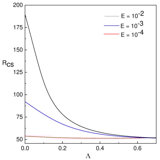
Figure 1. The effect of $\mathsf{\Lambda }$ and E on $R_{cs}$.

The linear stability theory adopts a less ambitious objective to ascertain when a flow is unstable to infinitesimal disturbances. It thus gives no prediction about transition promoted by sufficiently large disturbance. The ultimate consequence of the instability is never completely determined by linear theory. Thus, in the present study, an attempt was made to understand the nonlinear convection in the presence of the Coriolis force and magnetic field.

4. Method of Solution

The solutions of steady non-linear equations were obtained by following the method proposed by Kuo [5]. These solutions converge more rapidly and are valid for larger temperature differences. In this method, the dependent variables are first expressed as infinite series of a set of orthogonal space functions. This approach to the solution sheds light on the problem of transition to turbulent convection, which happens at a larger temperature difference. An expansion parameter ($\epsilon$), is defined by [5]:

$$\begin{array}{c}\hfill {\epsilon }^2=\frac{R-R_{cs}}{R}.\end{array}$$

(25)

Note that $\epsilon$ is less than one for all values of $\mathit{R}$. The solution of Equations (13)–(17) are written as

$$\begin{array}{c}\hfill f=\epsilon f_1+{\epsilon }^2{f}_2+{\epsilon }^3{f}_3+{\epsilon }^4{f}_4+{\epsilon }^5{f}_5+{\epsilon }^6{f}_6+\cdots ,\end{array}$$

(26)

where

$$f=f(U,W,\theta ,b_X,b_Z,{\omega }_Z,J_Z).$$

According to Equation (25), R is given by

$$\begin{array}{c}\hfill R=\frac{R_{cs}}{1-{\epsilon }^2},\end{array}$$

(27)

expanding Equation (27) in the power series of $\epsilon$ or by applying the finite formula

$$\begin{array}{c}\hfill R=R_{cs}+R_{os}({\epsilon }^2+{\epsilon }^4+{\epsilon }^6+\cdots +{\epsilon }^{2s}),\end{array}$$

(28)

where

$$\begin{array}{c}\hfill R_{os}=\frac{R_{cs}}{1-{\epsilon }^{2s}},s=1,2,3\cdots \end{array}$$

(29)

By introducing Equations (26) and (28) in Equation (18), we obtain for the different $\epsilon$ orders, a sequence of linear non homogeneous differential equations as

$$\begin{array}{c}\hfill O\left(\epsilon \right):\left({\mathcal{L}}_1+{\mathcal{L}}_2+{\mathcal{L}}_3+{\mathcal{L}}_4\right)W_1+R_{cs}({\mathcal{L}}_5+{\mathcal{L}}_6)W_1=0,\end{array}$$

(30)

$$\begin{array}{c}\hfill O\left({\epsilon }^2\right):\left({\mathcal{L}}_1+{\mathcal{L}}_2+{\mathcal{L}}_3+{\mathcal{L}}_4\right)W_2+R_{cs}({\mathcal{L}}_5+{\mathcal{L}}_6)W_2=0,\end{array}$$

(31)

$$\begin{array}{c}\hfill O\left({\epsilon }^3\right):\left({\mathcal{L}}_1+{\mathcal{L}}_2+{\mathcal{L}}_3+{\mathcal{L}}_4\right)W_i+R_{cs}({\mathcal{L}}_5+{\mathcal{L}}_6)W_i+R_{os}({\mathcal{L}}_5+{\mathcal{L}}_6)W_{i-2}\\ \hfill +R_{os}({\mathcal{L}}_5+{\mathcal{L}}_6)W_{i-4}=R_{cs}{\mathcal{N}}_1+{\mathcal{N}}_2+{\mathcal{N}}_3+{\mathcal{N}}_4+{\mathcal{N}}_5,\mathrm{for}i=3.\end{array}$$

(32)

Similarly, at the orders $O\left({\epsilon }^4\right)$, $O\left({\epsilon }^5\right)$, we obtain

$$\begin{array}{c}\hfill \left({\mathcal{L}}_1+{\mathcal{L}}_2+{\mathcal{L}}_3+{\mathcal{L}}_4\right)W_i+R_{cs}({\mathcal{L}}_5+{\mathcal{L}}_6)W_i+R_{os}({\mathcal{L}}_5+{\mathcal{L}}_6)W_{i-2}\\ \hfill +R_{os}({\mathcal{L}}_5+{\mathcal{L}}_6)W_{i-4}=(R_{cs}+R_{os}){\mathcal{N}}_1+{\mathcal{N}}_2+{\mathcal{N}}_3+{\mathcal{N}}_4+{\mathcal{N}}_5,\mathrm{for}i=4,5.\end{array}$$

(33)

In general,

$$\begin{array}{c}\hfill \left({\mathcal{L}}_1+{\mathcal{L}}_2+{\mathcal{L}}_3+{\mathcal{L}}_4\right)W_i+R_{cs}({\mathcal{L}}_5+{\mathcal{L}}_6)W_i+R_{os}({\mathcal{L}}_5+{\mathcal{L}}_6)W_{i-2}\\ \hfill +R_{os}({\mathcal{L}}_5+{\mathcal{L}}_6)W_{i-4}=(R_{cs}+2R_{os}){\mathcal{N}}_1+{\mathcal{N}}_2+{\mathcal{N}}_3+{\mathcal{N}}_4+{\mathcal{N}}_5,\mathrm{for}i\ge 6.\end{array}$$

(34)

Here ${\mathcal{L}}_i$, $i=1,2,3,4,5,6$ is the linear operator and ${\mathcal{N}}_i$, $i=1,2,3,4,5$ represents the nonlinear terms and are functions of $W_i$, ${\theta }_i$, ${b_X}_i$, ${b_Z}_i$, ${{\omega }_Z}_i$, and ${J_Z}_i$. The auxiliary equations for temperature field are given by

$$\begin{array}{c}\hfill \left(\frac{\partial }{\partial t}-{\nabla }^2\right){\theta }_1=q{W}_1,\end{array}$$

(35)

$$\begin{array}{c}\hfill \left(\frac{\partial }{\partial t}-{\nabla }^2\right){\theta }_2+({\overrightarrow{V}}_1·\nabla ){\theta }_1=q{W}_2.\end{array}$$

(36)

In general,

$$\begin{array}{c}\hfill \left(\frac{\partial }{\partial t}-{\nabla }^2\right){\theta }_i+\sum _{l=1}^{i-1}({\overrightarrow{V}}_l·\nabla ){\theta }_{i-l}=q{W}_i,\mathrm{for}i\ge 3.\end{array}$$

(37)

The auxiliary equations for the magnetic field

$$\begin{array}{c}\hfill \left(\frac{\partial }{\partial t}-{\nabla }^2\right)b_{X_1}=\frac{\partial U_1}{\partial X}.\end{array}$$

(38)

In general,

$$\begin{array}{c}\hfill \left(\frac{\partial }{\partial t}-{\nabla }^2\right)b_{Xi}=\frac{\partial U_i}{\partial X}+\frac{\partial }{\partial Y}\left(U_1{b}_{Y_{i-1}}+\cdots +U_{i-1}{b}_{Y_1}-V_1{b}_{X_{i-1}}\cdots +V_{i-1}{b}_{X_1}\right)\\ \hfill +\frac{\partial }{\partial Z}\left(U_1{b}_{Z_{i-1}}+\cdots +U_{i-1}{b}_{Z_1}-W_1{b}_{X_{i-1}}\cdots +W_{i-1}{b}_{X_1}\right),\mathrm{for}i\ge 2,\end{array}$$

(39)

and

$$\begin{array}{c}\hfill \left(\frac{\partial }{\partial t}-{\nabla }^2\right)b_{Z_1}=\frac{\partial W_1}{\partial X}.\end{array}$$

(40)

In general written as:

$$\begin{array}{c}\hfill \left(\frac{\partial }{\partial t}-{\nabla }^2\right)b_{Z_i}=\frac{\partial W_i}{\partial X}-\frac{\partial }{\partial X}\left(U_1{b}_{Z_{i-1}}+\cdots +U_{i-1}{b}_{Z_1}-W_1{b}_{X_{i-1}}\cdots +W_{i-1}{b}_{X_1}\right)\\ \hfill -\frac{\partial }{\partial Y}\left(V_1{b}_{Z_{i-1}}+\cdots +V_{i-1}{b}_{Z_1}-W_1{b}_{Y_{i-1}}\cdots +W_{i-1}{b}_{Y_1}\right)\mathrm{for}i\ge 2.\end{array}$$

(41)

Likewise, the auxiliary equations for vorticity are

$$\begin{array}{c}\hfill E{\nabla }^2{\omega }_{Z_1}=-\frac{\partial W_1}{\partial Z}-\mathsf{\Lambda }\frac{\partial J_{Z_1}}{\partial X},\end{array}$$

(42)

in general,

$$\begin{array}{c}\hfill E{\nabla }^2{\omega }_{Z_i}=-\frac{\partial W_i}{\partial Z}-\mathsf{\Lambda }\frac{\partial J_{Z_i}}{\partial X}-\mathsf{\Lambda }\frac{\partial }{\partial X}{b}_{X_1}\left(\frac{\partial b_{Y_{i-1}}}{\partial X}-\frac{\partial b_{X_{i-1}}}{\partial Y}\right)+\cdots -\mathsf{\Lambda }\frac{\partial }{\partial X}{b}_{X_{i-1}}\left(\frac{\partial b_{Y_1}}{\partial X}-\frac{\partial b_{X_1}}{\partial Y}\right)\\ \hfill +\mathsf{\Lambda }\frac{\partial }{\partial X}{b}_{Z_1}\left(\frac{\partial b_{Z_{i-1}}}{\partial Y}-\frac{\partial b_{Y_{i-1}}}{\partial Z}\right)+\cdots +\mathsf{\Lambda }\frac{\partial }{\partial X}{b}_{Z_{i-1}}\left(\frac{\partial b_{Z_1}}{\partial Y}-\frac{\partial b_{Y_1}}{\partial Z}\right)\\ \hfill +\mathsf{\Lambda }\frac{\partial }{\partial Y}{b}_{Z_1}\left(\frac{\partial b_{X_{i-1}}}{\partial Z}-\frac{\partial b_{Z_{i-1}}}{\partial X}\right)+\cdots -\mathsf{\Lambda }\frac{\partial }{\partial Y}{b}_{Z_{i-1}}\left(\frac{\partial b_{X_1}}{\partial Z}-\frac{\partial b_{Z_1}}{\partial X}\right)\\ \hfill +\mathsf{\Lambda }\frac{\partial }{\partial Y}{b}_{Y_1}\left(\frac{\partial b_{Y_{i-1}}}{\partial X}-\frac{\partial b_{X_{i-1}}}{\partial Y}\right)+\cdots +\mathsf{\Lambda }\frac{\partial }{\partial Y}{b}_{Y_{i-1}}\left(\frac{\partial b_{Y_1}}{\partial X}-\frac{\partial b_{X_1}}{\partial Y}\right),\mathrm{for}i\ge 2,\end{array}$$

(43)

and

$$\begin{array}{c}\hfill \left(\frac{\partial }{\partial t}-{\nabla }^2\right)J_{Z_1}=\frac{\partial {\omega }_{Z_1}}{\partial X},\end{array}$$

(44)

in general written as:

$$\begin{array}{c}\hfill \left(\frac{\partial }{\partial t}-{\nabla }^2\right)J_{Z_i}=\frac{\partial {\omega }_{Z_i}}{\partial X}+\frac{{\partial }^2}{\partial X\partial Z}\left(V_1{b}_{Z_{i-1}}+\cdots +V_{i-1}{b}_{Z_1}-W_{i-1}{b}_{Y_1}-\cdots -W_1{b}_{Y_{i-1}}\right)\\ \hfill +\frac{{\partial }^2}{\partial Y\partial Z}\left(W_{i-1}{b}_{X_1}+\cdots +W_1{b}_{X_1}-U_1{b}_{Z_{i-1}}-\cdots -U_{i-1}{b}_{Z_1}\right)\\ \hfill +{\nabla }_h^2\left(V_1{b}_{X_{i-1}}+\cdots +V_{i-1}{b}_{X_1}-U_{i-1}{b}_{Y_1}-\cdots -U_1{b}_{Y_{i-1}}\right),\mathrm{for}i\ge 2.\end{array}$$

(45)

4.1. Approximate Solutions

The approximate solutions $U,W,\theta$, $b_X$, and $b_Z$ are attained in terms of the amplitudes near the onset of stationary convection. The horizontal two boundaries are stress-free, all the space functions $U,W,\theta$, $b_X$, and $b_Z$ are sine and cosine functions. Thus, from Equations (30), (35), (42), and (44) we have, to the first order periodic solutions as,

$$\begin{array}{ccc}\hfill & & W_1=A_{1}cosaXsin\pi Z,\hfill \\ & & {\theta }_1=\frac{q{A}_1}{{\pi }^2+a^2}cosaXsin\pi Z,\hfill \end{array}$$

$$\begin{array}{c}\hfill \\ & & b_{X_1}=-\frac{\pi A_1}{{\pi }^2+a^2}cosaXcos\pi Z,\hfill \\ & & b_{Z_1}=-\frac{a{A}_1}{{\pi }^2+a^2}sinaXsin\pi Z,\hfill \end{array}$$

(46)

where the nonlinear terms are used to calculate the amplitude $A_1$. Normally, the terms in Equation (26) are written as

$$\begin{array}{c}\hfill W_i=A_{i}cosaXsin\pi Z+\sum _{p_1,q_1}{W}_{p_1{q}_1}^{\left(i\right)}cos{p}_{1}aXsin{q}_1\pi Z,\end{array}$$

(47)

$$\begin{array}{c}\hfill U_i=\frac{1}{a^2}\frac{{\partial }^2{W}_i}{\partial Z\partial X},V_i=\frac{1}{a^2}\frac{{\partial }^2{W}_i}{\partial Z\partial Y},{\omega }_{Z_i}=\frac{\partial V_i}{\partial X},\end{array}$$

(48)

$$\begin{array}{c}\hfill {\theta }_i=\frac{q{A}_i}{{\pi }^2+a^2}cosaXsin\pi Z+\sum _{p_1,q_1}{\theta }_{p_1{q}_1}^{\left(i\right)}cos{p}_{1}aXsin{q}_1\pi Z,\end{array}$$

(49)

$$\begin{array}{c}\hfill b_{X_i}=-\frac{\pi A_i}{({\pi }^2+a^2)}cosaXcos\pi Z+\sum _{p_1,q_1}{b_X}_{p_1{q}_1}^{\left(i\right)}cos{p}_{1}aXcos{q}_1\pi Z,\end{array}$$

(50)

$$\begin{array}{c}\hfill b_{Z_i}=-\frac{a{A}_i}{({\pi }^2+a^2)}sinaXsin\pi Z+\sum _{p_1,q_1}{b_Z}_{p_1{q}_1}^{\left(i\right)}sin{p}_{1}aXsin{q}_1\pi Z,\end{array}$$

(51)

where $W_{p_1{q}_1}^{\left(i\right)}$, ${\theta }_{p_1{q}_1}^{\left(i\right)}$, ${b_X}_{p_1{q}_1}^{\left(i\right)}$, and ${b_Z}_{p_1{q}_1}^{\left(i\right)}$ are nonlinear functions of $A_1$, $A_2$, $A_3$,…$A_{i-1}$. The unknown functions $W_{p_1{q}_1}^{\left(i\right)}$, ${\theta }_{p_1{q}_1}^{\left(i\right)}$, ${b_X}_{p_1{q}_1}^{\left(i\right)}$, and ${b_Z}_{p_1{q}_1}^{\left(i\right)}$ are calculated by substituting the Equations (47)–(51) in Equation (18).

4.2. Evaluation of Amplitude $A_1$

To obtain the second order solutions $W_2$, ${\theta }_2$, $b_{X_2}$, and $b_{Z_2}$, the nonlinear term $\mathcal{N}$ is solved and Equation (31) is obtained. With $\mathcal{N}$ = 0, $\mathcal{L}$$\mathit{W}$${}_2$ = 0 and

$$\begin{array}{c}\hfill W_{02}^{\left(2\right)}=0,{\theta }_{02}^{\left(2\right)}=\frac{q{A}_1^2}{8\pi ({\pi }^2+a^2)}and{b_X}_{02}^{\left(2\right)}=\frac{A_1^2}{4({\pi }^2+a^2)},{b_Z}_{02}^{\left(2\right)}=0.\end{array}$$

(52)

The unknown functions $W_2$, ${\theta }_2$, $b_{X_2}$, and $b_{Z_2}$ are obtained from Equations (31), (36), (39), and (41), respectively, and are given by

$$\begin{array}{ccc}\hfill & & W_2=A_{2}cosaXsin\pi Z,\hfill \\ & & {\theta }_2=\frac{q{A}_2}{{\pi }^2+a^2}cosaXsin\pi Z+{{\theta }_{02}}^{\left(2\right)}{A_1}^{2}sin2\pi Z,\hfill \\ & & b_{X_2}=-\frac{\pi A_2}{{\pi }^2+a^2}cosaXcos\pi Z+{{b_X}_{02}}^{\left(2\right)}{A_1}^{2}cos2\pi Z,\hfill \\ & & b_{Z_2}=-\frac{a{A}_2}{{\pi }^2+a^2}sinaXsin\pi Z.\hfill \end{array}$$

(53)

From Equation (32) for $i=3$ the amplitude ${\mathit{A}}_{\mathit{1}}$ is calculated. After using the first and second order solutions, we write Equation (32) as

$$\begin{array}{ccc}\hfill & & \left({\mathcal{L}}_1+{\mathcal{L}}_2+{\mathcal{L}}_3+{\mathcal{L}}_4\right)W_3+R_{cs}({\mathcal{L}}_5+{\mathcal{L}}_6)W_3\hfill \\ & & =-R_{os}[qE{({\pi }^2+a^2)}^3{a}^2+q\mathsf{\Lambda }({\pi }^2+a^2)a^4]\hfill \\ & & A_{1}cosaXsin\pi Z-R_{cs}[E{d_2}^3{a}^2+\mathsf{\Lambda }{d}_2{a}^4]\pi {{\theta }_{{}_{02}}}^{\left(2\right)}{A_1}^{3}cosaXsin\pi Z\hfill \end{array}$$

$$\begin{array}{c}\hfill \\ & & -[a^2{{b_X}_{02}}^{\left(2\right)}E\mathsf{\Lambda }q{d_2}^4+a^4{{b_X}_{02}}^{\left(2\right)}{\mathsf{\Lambda }}^{2}q{d_2}^2]\frac{{A_1}^3}{2}cosaXsin\pi Z\hfill \\ & & +R_{cs}[E{(a^2+9{\pi }^2)}^3{a}^2+\mathsf{\Lambda }(a^2+9{\pi }^2)a^4]\pi {{\theta }_{{}_{02}}}^{\left(2\right)}{A_1}^{3}cosaXsin3\pi Z\hfill \\ & & +[a^2{{b_X}_{02}}^{\left(2\right)}E\mathsf{\Lambda }q{(a^2+9{\pi }^2)}^4+a^4{{b_X}_{02}}^{\left(2\right)}{\mathsf{\Lambda }}^{2}q{(a^2+9{\pi }^2)}^2]\frac{{A_1}^3}{2}cosaXsin3\pi Z\hfill \\ & & -[\frac{2{\pi }^2{a}^2}{d^2}{b_{X02}}^{\left(2\right)}-a^2\frac{{b_{X02}}^{\left(2\right)}}{2}]{A_1}^{3}cosaXsin\pi Z\hfill \\ & & +[\frac{2{\pi }^2{a}^2}{d^2}{b_{X02}}^{\left(2\right)}-a^2\frac{{b_{X02}}^{\left(2\right)}}{\left(2\right)}]{A_1}^{3}cosaXsin3\pi Z,\hfill \end{array}$$

(54)

where $d_2=a^2+{\pi }^2$. By solving the above equation, ${\mathit{A}}_{\mathit{1}}$ is given by

$$\begin{array}{c}\hfill A_1=-\frac{\sqrt{\left(2\mathsf{\Lambda }{{{\mathit{b}}_{\mathit{X}}}_{\mathit{02}}}^{\left(\mathit{2}\right)}{\pi }^2-\mathsf{\Lambda }{{{\mathit{b}}_{\mathit{X}}}_{\mathit{02}}}^{\left(\mathit{2}\right)}{\mathit{d}}_{\mathit{2}}-\pi {\mathit{R}}_{\mathit{cs}}{{\theta }_{02}}^{\left(2\right)}\right){\mathit{R}}_{\mathit{os}}q}}{2\mathsf{\Lambda }{{{\mathit{b}}_{\mathit{X}}}_{\mathit{02}}}^{\left(\mathit{2}\right)}{\pi }^2-\mathsf{\Lambda }{{{\mathit{b}}_{\mathit{X}}}_{\mathit{02}}}^{\left(\mathit{2}\right)}{\mathit{d}}_{\mathit{2}}-\pi {\mathit{R}}_{\mathit{cs}}{{\theta }_{{}_{02}}}^{\left(2\right)}}.\end{array}$$

(55)

The unknown functions $W_3$, ${\theta }_3$, $b_{X_3}$, and $b_{Z_3}$ are obtained from Equations (32), (37), (39), and (41), respectively,

$$\begin{array}{ccc}\hfill & & W_3=A_{3}cosaXsin\pi Z+{W_{13}}^{\left(3\right)}{A_1}^{3}cosaXsin3\pi Z,\hfill \\ & & {\theta }_3=\left(\frac{q{A}_3}{{\pi }^2+a^2}+{{\theta }_{11}}^{\left(3\right)}{A_1}^3\right)cosaXsin\pi Z\hfill \\ & & +{{\theta }_{13}}^{\left(3\right)}{A_1}^{3}cosaXsin3\pi Z,\hfill \\ & & b_{X_3}=\left(-\frac{\pi A_3}{{\pi }^2+a^2}+{{b_X}_{11}}^{\left(3\right)}{A_1}^3\right)cosaXcos\pi Z\hfill \\ & & +{{b_X}_{13}}^{\left(3\right)}{A_1}^{3}cosaXcos3\pi Z,\hfill \\ & & b_{Z_3}=\left(-\frac{a{A}_3}{{\pi }^2+a^2}+{{b_Z}_{11}}^{\left(3\right)}{A_1}^3\right)sinaXsin\pi Z\hfill \\ & & +{{b_Z}_{13}}^{\left(3\right)}{A_1}^{3}sinaXsin3\pi Z.\hfill \end{array}$$

(56)

where

$$W_{13}^{\left(3\right)}=\frac{1}{{\mathit{D}}_{\mathit{13}}}\left({\mathit{R}}_{\mathit{cs}}\left(q\mathsf{\Lambda }{\mathit{d}}_{\mathit{13}}{a}^4+Eq{{\mathit{d}}_{\mathit{13}}}^3{a}^2\right)\pi {{\theta }_{02}}^{\left(2\right)}\right)$$

$$+\frac{1}{{\mathit{D}}_{\mathit{13}}}\left(\left(\frac{1}{2}{a}^{2}E\mathsf{\Lambda }q{{\mathit{d}}_{\mathit{13}}}^4+\frac{1}{2}{a}^4{\mathsf{\Lambda }}^{2}q{{\mathit{d}}_{\mathit{13}}}^2\right){{\mathit{b}}_{\mathit{X}\mathit{02}}}^{\left(\mathit{2}\right)}+\left(2\frac{{\pi }^2{a}^2}{{\mathit{d}}_{\mathit{2}}}-\frac{1}{2}{a}^2\right){\mathit{b}}_{\mathit{X}\mathit{02}}^{\left(\mathit{2}\right)}\right),$$

$${\theta }_{11}^{\left(3\right)}=\frac{\pi {\theta }_{02}^{\left(2\right)}}{{\mathit{d}}_{\mathit{2}}},{\theta }_{13}^{\left(3\right)}=\frac{-\pi {\theta }_{02}^{\left(2\right)}+{\mathit{W}}_{\mathit{13}}^{\left(\mathit{3}\right)}q}{{\mathit{d}}_{\mathit{13}}},$$

and

$${b_X}_{11}^{\left(3\right)}=\frac{\pi {{\mathit{b}}_{\mathit{X}}}_{\mathit{02}}^{\left(\mathit{2}\right)}}{2{\mathit{d}}_{\mathit{2}}},{b_X}_{13}^{\left(3\right)}=-\frac{3\pi {\mathit{W}}_{\mathit{13}}^{\left(\mathit{3}\right)}}{{\mathit{d}}_{\mathit{2}}}-\frac{3\pi {{\mathit{b}}_{\mathit{X}}}_{\mathit{02}}^{\left(\mathit{2}\right)}}{2{\mathit{d}}_{\mathit{2}}},$$

$${b_Z}_{11}^{\left(3\right)}=\frac{a{{\mathit{b}}_{\mathit{X}}}_{\mathit{02}}^{\left(\mathit{2}\right)}}{2{\mathit{d}}_{\mathit{2}}},{b_Z}_{13}^{\left(3\right)}=-\frac{a{\mathit{W}}_{\mathit{13}}^{\left(\mathit{3}\right)}}{{\mathit{d}}_{\mathit{2}}}-\frac{a{{\mathit{b}}_{\mathit{X}}}_{\mathit{02}}^{\left(\mathit{2}\right)}}{2{\mathit{d}}_{\mathit{2}}},$$

$$D_{13}=-9q{\pi }^2{d}_{13}^3-E^{2}q{d}_{13}^6-2E\mathsf{\Lambda }q{a}^2{d}_{13}^4$$

$$-{\mathsf{\Lambda }}^2{q}^2{a}^4{d}_{13}^2+{\mathit{R}}_{\mathit{cs}}\left(q{a}^{2}E{d}_{13}^3+q\mathsf{\Lambda }{a}^4{d}_{13}\right),$$

where $d_{13}=a^2+9{\pi }^2$. This iterative procedure is continued to find $A_2$ to $A_6$ and the equivalent $W_i$, ${\theta }_i$, $b_{X_i}$, $b_{Z_i}$, ${\omega }_{Z_i}$, and $J_{Z_i}$, etc.

4.3. Calculation of $A_2$ and $A_3$

Initially, Equation (33) is simplified for $i=4$, i.e.,

$$\begin{array}{c}\hfill ({\mathcal{L}}_1+{\mathcal{L}}_2+{\mathcal{L}}_3+{\mathcal{L}}_4+R_{cs}({\mathcal{L}}_5+{\mathcal{L}}_6))W_4+R_{os}({\mathcal{L}}_5+{\mathcal{L}}_6)W_2\\ \hfill =(R_{cs}+R_{os}){\mathcal{N}}_1+{\mathcal{N}}_2+{\mathcal{N}}_3+{\mathcal{N}}_4+{\mathcal{N}}_5.\end{array}$$

(57)

The nonlinear terms ${\mathcal{N}}_i$, $i=1,2,3,4,5$ are analyzed by using the Equations (46), (53) and (56). Solving the above Equation (57), we obtain $A_2$ = 0. This indicates that every second order approximate solutions vanish except for ${\theta }_{02}^{\left(2\right)}$ and $b_{X02}^{\left(2\right)}$ as shown in Equation (52). Therefore, Equation (57) decreases to

$$\begin{array}{ccc}\hfill & & ({\mathcal{L}}_1+{\mathcal{L}}_2+{\mathcal{L}}_3+{\mathcal{L}}_4+R_{cs}({\mathcal{L}}_5+{\mathcal{L}}_6))W_4=K_1{A_1}^{4}cos2aXsin4\pi Z\hfill \\ & & +K_2{A_1}^{4}cos2aXsin2\pi Z+K_3{A}_1{A}_{3}cos2aXsin2\pi Z.\hfill \end{array}$$

(58)

The approximate solutions $W_4$, ${\theta }_4$, $b_{X_4},b_{Z_4}$ are evaluated by Equations (33), (37), (39) and (41) and those are given by

$$\begin{array}{ccc}\hfill & & W_4=A_{4}cosaXsin\pi Z+K_4{A}_1^{4}cos2aXsin4\pi Z\hfill \\ & & +K_5{A}_1^{4}cos2aXsin2\pi Z+K_6{A}_1{A}_{3}cos2aXsin2\pi Z,\hfill \\ & & {\theta }_4=\frac{q}{(a^2+{\pi }^2)}{A}_{4}cosaXsin\pi Z+K_7{A}_1{A}_{3}sin2\pi Z\hfill \\ & & +K_8{A}_1^{4}sin2\pi Z+K_9{A}_1^{4}cos2aXsin2\pi Z+K_{10}{A}_1^{4}cos2aXsin4\pi Z\hfill \\ & & +K_{11}{A}_1^{4}sin4\pi Z+K_{12}{A}_1{A}_{3}cos2aXsin2\pi Z,\hfill \\ & & b_{X_4}=\frac{-\pi }{(a^2+{\pi }^2)}{A}_{4}cosaXcos\pi Z+K_{13}{A}_1^{4}cos2aXcos4\pi Z\hfill \\ & & +K_{14}{A}_1^{4}cos2aXcos2\pi Z+K_{15}{A}_1{A}_{3}cos2aXcos2\pi Z,\hfill \\ & & b_{Z_4}=\frac{-a}{(a^2+{\pi }^2)}{A}_{4}sinaXsin\pi Z+K_{16}{A}_1^{4}sin2aXsin4\pi Z\hfill \\ & & +K_{17}{A}_1^{4}sin2aXsin2\pi Z+K_{18}{A}_1{A}_{3}sin2aXsin2\pi Z.\hfill \end{array}$$

(59)

To determine the value of $A_3$, Equation (33) is solved for $\mathit{i}$ = 5, and is given by

$$\begin{array}{c}\hfill ({\mathcal{L}}_1+{\mathcal{L}}_2+{\mathcal{L}}_3+{\mathcal{L}}_4+R_{cs}({\mathcal{L}}_5+{\mathcal{L}}_6))W_5+R_{os}({\mathcal{L}}_5+{\mathcal{L}}_6)(W_3+W_1)\\ \hfill =(R_{cs}+R_{os}){\mathcal{N}}_1+{\mathcal{N}}_2+{\mathcal{N}}_3+{\mathcal{N}}_4+{\mathcal{N}}_5.\end{array}$$

(60)

Evaluating $A_3$ from Equations (46), (53), (56), (59) and (60) we obtain,

$$\begin{array}{c}\hfill A_3=\frac{S_1}{S_2},\end{array}$$

(61)

where

$$S_1=-{{\mathit{A}}_{\mathit{1}}}^5\left({\mathsf{\Lambda }}^{2}q{{\mathit{d}}_{\mathit{2}}}^2{a}^3+E\mathsf{\Lambda }q{{\mathit{d}}_{\mathit{2}}}^{4}a\right)\left(\frac{-\pi K_{17}}{4a}+\frac{K_{14}}{4}-\frac{b_{X02}^{\left(2\right)}{W}_{13}^3}{2}-\frac{3\pi K_5}{\mathit{4}{\mathit{d}}_{\mathit{2}}}\right)a$$

$$+{{\mathit{A}}_{\mathit{1}}}^5\left({\mathsf{\Lambda }}^{2}q{{\mathit{d}}_{\mathit{2}}}^2{a}^2+E\mathsf{\Lambda }q{{\mathit{d}}_{\mathit{2}}}^4\right)\left(-\frac{a\left(2\pi K_{14}+2a{K}_{17}\right)}{4{\mathit{d}}_{\mathit{2}}}-\pi {\mathit{b}}_{\mathit{X}\mathit{02}}^{\left(\mathit{2}\right)}{b}_{Z11}^{\left(3\right)}-\pi b_{X02}^{\left(2\right)}{b}_{Z13}^{\left(3\right)}+K_{17}\right)\pi a$$

$$+{{\mathit{A}}_{\mathit{1}}}^5{a}^2\left({\mathsf{\Lambda }}^{2}q{{\mathit{d}}_{\mathit{2}}}^2{a}^2+E\mathsf{\Lambda }q{{\mathit{d}}_{\mathit{2}}}^4\right)\left(\frac{\pi \left(2\pi K_{14}+2a{K}_{17}\right)}{4{\mathit{d}}_{\mathit{2}}}+\frac{b_{X02}^{\left(2\right)}}{2}\left(\pi b_{X11}^{\left(3\right)}+a{b}_{Z11}^{\left(3\right)}\right)\right)$$

$$-{{\mathit{A}}_{\mathit{1}}}^5{a}^2\left({\mathsf{\Lambda }}^{2}q{{\mathit{d}}_{\mathit{2}}}^2{a}^2+E\mathsf{\Lambda }q{{\mathit{d}}_{\mathit{2}}}^4\right)\left(\frac{b_{X02}^{\left(2\right)}}{2}\left(3\pi b_{X13}^{\left(3\right)}+a{b}_{Z13}^{\left(3\right)}\right)+\pi b_{X02}^{\left(2\right)}{b}_{X11}^{\left(3\right)}-\pi b_{X02}^{\left(2\right)}{b}_{X13}^{\left(3\right)}\right)$$

$$+\left(q\mathsf{\Lambda }{\mathit{d}}_{\mathit{2}}{a}^4+Eq{{\mathit{d}}_{\mathit{2}}}^3{a}^2\right)\left(\pi {\theta }_{02}^{\left(2\right)}{W}_{13}^{\left(3\right)}-\frac{3\pi q{K}_5}{4{\mathit{d}}_{\mathit{2}}}-\pi \frac{K_9}{4}-\pi K_8\right){{\mathit{A}}_{\mathit{1}}}^5{\mathit{R}}_{\mathit{cs}}$$

$$+\left(q\mathsf{\Lambda }{\mathit{d}}_{\mathit{2}}{a}^4+Eq{{\mathit{d}}_{\mathit{2}}}^3{a}^2\right)\left(\pi {\theta }_{02}^{\left(2\right)}{W}_{13}^{\left(3\right)}-\frac{3\pi q{K}_5}{4{\mathit{d}}_{\mathit{2}}}-\pi K_9-\pi K_8\right){{\mathit{A}}_{\mathit{1}}}^5{\mathit{R}}_{\mathit{os}}$$

$$-\mathsf{\Lambda }{\mathit{R}}_{\mathit{os}}{a}^4{\mathit{d}}_{\mathit{2}}{q}^2-E{\mathit{R}}_{\mathit{os}}{a}^2{{\mathit{d}}_{\mathit{2}}}^3{q}^2-{{\mathit{A}}_{\mathit{1}}}^5{a}^2\left({\mathsf{\Lambda }}^{2}q{{\mathit{d}}_{\mathit{2}}}^2{a}^2+E\mathsf{\Lambda }q{{\mathit{d}}_{\mathit{2}}}^4\right)K_{14},$$

and

$$S_2=-\left(q\mathsf{\Lambda }{\mathit{d}}_{\mathit{2}}{a}^4+Eq{{\mathit{d}}_{\mathit{2}}}^3{a}^2\right)\left(-\pi K_8-\pi {\theta }_{02}^{\left(2\right)}-\pi q\frac{3K_5}{4}\right){{\mathit{A}}_{\mathit{1}}}^2{\mathit{R}}_{\mathit{cs}}$$

$$-\left(q\mathsf{\Lambda }{\mathit{d}}_{\mathit{2}}{a}^4+Eq{{\mathit{d}}_{\mathit{2}}}^3{a}^2\right)\left(-\pi K_8-\pi {\theta }_{02}^{\left(2\right)}-\pi q\frac{3K_5}{4}\right){{\mathit{A}}_{\mathit{1}}}^2{\mathit{R}}_{\mathit{os}}$$

$$+{{\mathit{A}}_{\mathit{1}}}^2\left({\mathsf{\Lambda }}^{2}q{{\mathit{d}}_{\mathit{2}}}^2{a}^3+E\mathsf{\Lambda }q{{\mathit{d}}_{\mathit{2}}}^{4}a\right)\left(\frac{b_{X02}^{\left(2\right)}}{2}-\frac{\pi K_{17}}{4a}+\frac{K_{14}}{4}-\frac{3\pi K_5}{4{\mathit{d}}_{\mathit{2}}}\right)a$$

$$-{{\mathit{A}}_{\mathit{1}}}^2\left({\mathsf{\Lambda }}^{2}q{{\mathit{d}}_{\mathit{2}}}^2{a}^2+E\mathsf{\Lambda }q{{\mathit{d}}_{\mathit{2}}}^4\right)\left(-\frac{a\left(2\pi K_{14}-2a{K}_{17}\right)}{4{\mathit{d}}_{\mathit{2}}}+\frac{\pi a{b}_{X02}^{\left(2\right)}}{{\mathit{d}}_{\mathit{2}}}+K_{17}\right)\pi a$$

$$-{{\mathit{A}}_{\mathit{1}}}^2\left({\mathsf{\Lambda }}^{2}q{{\mathit{d}}_{\mathit{2}}}^2{a}^2+E\mathsf{\Lambda }q{{\mathit{d}}_{\mathit{2}}}^4\right)\left(\frac{\pi \left(2\pi K_{14}+2a{K}_{17}\right)}{4{\mathit{d}}_{\mathit{2}}}-\frac{b_{X02}^{\left(2\right)}}{2}\right)a^2$$

$$-{{\mathit{A}}_{\mathit{1}}}^2\left({\mathsf{\Lambda }}^{2}q{{\mathit{d}}_{\mathit{2}}}^2{a}^2+E\mathsf{\Lambda }q{{\mathit{d}}_{\mathit{2}}}^4\right)\left(\frac{{\pi }^2{b}_{X02}^{\left(2\right)}}{{\mathit{d}}_{\mathit{2}}}-K_{14}\right)a^2+\mathsf{\Lambda }{\mathit{R}}_{\mathit{os}}{a}^4{\mathit{d}}_{\mathit{2}}{q}^2+E{\mathit{R}}_{\mathit{os}}{a}^2{{\mathit{d}}_{\mathit{2}}}^3{q}^2.$$

The amplitude ${\mathit{A}}_{\mathit{3}}$ is determined by using the first, second, third and fourth order approximate solutions. From Equations (60), (37), (39) and (41), the fifth order approximate solutions are obtained

$$\begin{array}{ccc}\hfill & & W_5={\mathit{A}}_{\mathit{5}}cosaXsin\pi Z\hfill \\ & & +\left(K_{19}{{\mathit{A}}_{\mathit{1}}}^5+K_{20}{{\mathit{A}}_{\mathit{1}}}^2{\mathit{A}}_{\mathit{3}}\right)cos3aXsin\pi Z\hfill \\ & & +\left(K_{21}{{\mathit{A}}_{\mathit{1}}}^3+K_{22}{{\mathit{A}}_{\mathit{1}}}^5+K_{23}{{\mathit{A}}_{\mathit{1}}}^2{\mathit{A}}_{\mathit{3}}\right)cosaXsin3\pi Z\hfill \\ & & +\left(K_{24}{{\mathit{A}}_{\mathit{1}}}^5+K_{25}{{\mathit{A}}_{\mathit{1}}}^2{\mathit{A}}_{\mathit{3}}\right)cos3aXsin3\pi Z\hfill \\ & & +K_{26}{{\mathit{A}}_{\mathit{1}}}^{5}cosaXsin5\pi Z+K_{27}{{\mathit{A}}_{\mathit{1}}}^{5}cos3aXsin5\pi Z,\hfill \end{array}$$

(62)

$$\begin{array}{ccc}\hfill & & {\theta }_5=\left(\frac{q{\mathit{A}}_{\mathit{5}}}{{\mathit{d}}_{\mathit{2}}}+K_{28}{{\mathit{A}}_{\mathit{1}}}^2{\mathit{A}}_{\mathit{3}}\right)cosaXsin\pi Z\hfill \\ & & +\left(K_{29}{{\mathit{A}}_{\mathit{1}}}^3+K_{30}{{\mathit{A}}_{\mathit{1}}}^5+K_{31}{{\mathit{A}}_{\mathit{1}}}^2{\mathit{A}}_{\mathit{3}}\right)cosaXsin3\pi Z\hfill \\ & & +\left(K_{32}{{\mathit{A}}_{\mathit{1}}}^5+K_{33}{{\mathit{A}}_{\mathit{1}}}^2{\mathit{A}}_{\mathit{3}}\right)cos3aXsin\pi Z\hfill \\ & & +\left(K_{34}{{\mathit{A}}_{\mathit{1}}}^5+K_{35}{{\mathit{A}}_{\mathit{1}}}^2{\mathit{A}}_{\mathit{3}}\right)cos3aXsin3\pi Z\hfill \\ & & +K_{36}{{\mathit{A}}_{\mathit{1}}}^{5}cosaXsin5\pi Z+K_{37}{{\mathit{A}}_{\mathit{1}}}^{5}cos3aXsin5\pi Z,\hfill \end{array}$$

(63)

$$\begin{array}{ccc}\hfill & & b_{X_5}=\left(-\frac{\pi {\mathit{A}}_{\mathit{5}}}{{\mathit{d}}_{\mathit{2}}}+K_{38}{{\mathit{A}}_{\mathit{1}}}^5\right)cosaXcos\pi Z\hfill \\ & & +\left(K_{39}{{\mathit{A}}_{\mathit{1}}}^3+K_{40}{{\mathit{A}}_{\mathit{1}}}^5+K_{41}{{\mathit{A}}_{\mathit{1}}}^2{\mathit{A}}_{\mathit{3}}\right)cosaXcos3\pi Z\hfill \\ & & +\left(K_{42}{{\mathit{A}}_{\mathit{1}}}^5+K_{43}{{\mathit{A}}_{\mathit{1}}}^2{\mathit{A}}_{\mathit{3}}\right)cos3aXcos\pi Z\hfill \end{array}$$

$$\begin{array}{c}\hfill \\ & & +\left(K_{44}{{\mathit{A}}_{\mathit{1}}}^5+K_{45}{{\mathit{A}}_{\mathit{1}}}^2{\mathit{A}}_{\mathit{3}}\right)cos3aXcos3\pi Z\hfill \\ & & +K_{46}{{\mathit{A}}_{\mathit{1}}}^{5}cosaXcos5\pi Z+K_{47}{{\mathit{A}}_{\mathit{1}}}^{5}cos3aXcos5\pi Z,\hfill \end{array}$$

(64)

$$\begin{array}{ccc}\hfill & & b_{Z_5}=\left(-\frac{a{\mathit{A}}_{\mathit{5}}}{{\mathit{d}}_{\mathit{2}}}+K_{48}{{\mathit{A}}_{\mathit{1}}}^5+K_{49}{{\mathit{A}}_{\mathit{1}}}^2{\mathit{A}}_{\mathit{3}}\right)sinaXsin\pi Z\hfill \\ & & +\left(K_{50}{{\mathit{A}}_{\mathit{1}}}^3+K_{51}{{\mathit{A}}_{\mathit{1}}}^5+K_{52}{{\mathit{A}}_{\mathit{1}}}^2{\mathit{A}}_{\mathit{3}}\right)sinaXsin3\pi Z\hfill \\ & & +\left(K_{53}{{\mathit{A}}_{\mathit{1}}}^5+K_{54}{{\mathit{A}}_{\mathit{1}}}^2{\mathit{A}}_{\mathit{3}}\right)sin3aXsin\pi Z\hfill \\ & & +\left(K_{55}{{\mathit{A}}_{\mathit{1}}}^5+K_{56}{{\mathit{A}}_{\mathit{1}}}^2{\mathit{A}}_{\mathit{3}}\right)sin3aXsin3\pi Z\hfill \\ & & +K_{57}{{\mathit{A}}_{\mathit{1}}}^{5}sinaXsin5\pi Z+K_{58}{{\mathit{A}}_{\mathit{1}}}^{5}sin3aXsin5\pi Z.\hfill \end{array}$$

(65)

Here the coefficients $K_i,i=1,2,\dots 58$ in Equations (58)–(65) are functions of $a,E,\mathsf{\Lambda },\mathrm{and}q$. The simplifications become more critical as $\epsilon$ order increases. Similarly, the simplification was carried until the eighth order of Equation (34) to calculate for $A_4$, $A_5$, and $A_6$. Proceeding as above, it can be observed that $A_2=A_4=A_6=0.$

5. Convective Heat Transport

The changes in the two-dimensional flow patterns are illustrated by the local Nusselt number, $N_L,$ distributions over the heated plate. The heat transport coefficient in terms of the $N_L$ is expressed as [16,25]

$$\begin{array}{c}\hfill N_L=\frac{\partial T}{\partial n},\end{array}$$

(66)

here n denotes the normal direction on a plane. The heat transport is measured by the average Nusselt number ($Nu$), which is independent of Z and is given by

$$\begin{array}{c}\hfill Nu=\overline{WT}-\frac{\partial \overline{T}}{\partial Z},\end{array}$$

(67)

here the bar indicates a horizontal mean. Using Equation (67), $Nu$ is obtained by integrating the expression over the boundary, $Z=0$ [16].

$$\begin{array}{c}\hfill Nu=\frac{1}{L}{\int }_0^{L}WT-\frac{\partial T}{\partial Z}{|}_{z=0}dX,\end{array}$$

(68)

where L is the normalized horizontal cell width.

5.1. Local Nusselt Number ($N_L$)

Figure 2a illustrates the changes of $N_L$ for distinct values of E with respect to X. In selected regions, the number of peaks and the location of maximum and minimum of $N_L$ values depend on E. The maximum of $N_L$ value is constant, as X increases for defined E. However, as E decreases, the number of peaks is increased in a selected region. Figure 2b illustrates the variation of $N_L$ for different $\mathsf{\Lambda }$ concerning to X. The location of the maximum $N_L$ value is independent of the dimensionless plate length but depends on $\mathsf{\Lambda }$. The existence of the number of peaks in the given region of X increases, as $\mathsf{\Lambda }$ increases. Figure 2b illustrates the heat that is transported from the fluid to the boundary is increased as $\mathsf{\Lambda }$ increase.

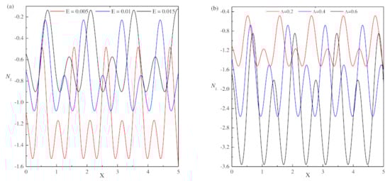
Figure 2. Variation of $N_L$ with respect to X. (a) $\mathsf{\Lambda }$ = 0.2 and q = 0.01 for different E, (b) E = 0.005 and q = 0.01 for different $\mathsf{\Lambda }$.

5.2. Average Nusselt Number ($Nu$)

The dependency of $Nu$ on the control parameters was studied near and away from the onset of stationary convection. Let $N{u}^{\left(2\right)}(s=1)$, $N{u}^{\left(4\right)}(s=2)$ and $N{u}^{\left(6\right)}(s=3)$, indicate the second-, fourth- and sixth-order approximations, for $Nu$, respectively. The second order approximation is given by

$$\begin{array}{c}\hfill N{u}^{\left(2\right)}=1+\frac{2q{R}_{os}}{2\mathsf{\Lambda }(a^2-{\pi }^2)+R_{cs}}.\end{array}$$

(69)

The approximations for $N{u}^{\left(4\right)}$ and $N{u}^{\left(6\right)}$ are lengthy, so it is not shown here to conserve space. The change of $Nu$ with respect to R is shown in Figure 3 for different values of E and $\mathsf{\Lambda }$. Figure 3a shows the effect of E on $Nu$ in the R plane for fixed $\mathsf{\Lambda }$ = 0.2 and q = 0.01. It illustrates that the rate of heat transfer is enhanced for decreasing E. Figure 3b shows the effect of $\mathsf{\Lambda }$ on heat transfer rate for fixed E = 0.005 and q = 0.01. The enhancement of heat transfer is observed for increasing $\mathsf{\Lambda }$ values. The small values of q are relevant to Earth’s outer core. It is very difficult to perform numerical simulations for small values of the physical parameters. For $q<1$ stationary convection is preferred [13]. Figure 3c shows that for $q<1$ and as q increases, the $Nu$ increase. Thus the effect of $q<1$ shows, the heat transfer rate are enhanced and accordingly the intensity of the flow rate also increase. The change of kinetic energy with respect to $R/R_{{}_{cs}}$ is represented in Figure 4. Figure 4a demonstrates the change in $Nu$ for various E values as well as for a fixed value of $\mathsf{\Lambda }=0.2$. The change in E produces small change in the potential energy, in comparison with the kinetic energy. Thus, the total energy decreases as E increase. Figure 4b shows the energy distribution for different $\mathsf{\Lambda }$ and for fixed $E=0.005$ and $q=0.01$. The amplifying values of $\mathsf{\Lambda }$ show that the total energy is also increased.

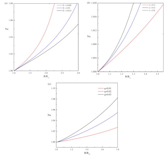
Figure 3. Dependence of Nussult number (Nu) on Rayleigh number ($R/R_{cs}$). (a) $\mathsf{\Lambda }$ = 0.2 and q = 0.01 for different E, (b) E = 0.005 and q = 0.01 for different $\mathsf{\Lambda }$, (c) E = 0.005 and $\mathsf{\Lambda }$ = 0.2 for different q.

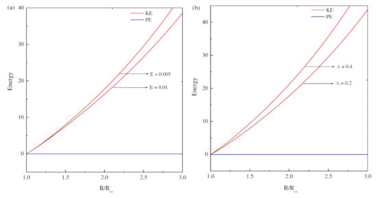
Figure 4. Dependence of kinetic energy and potential energy on Rayleigh number ($R/R_{cs}$) are plotted. (a) $\mathsf{\Lambda }=0.2$ and $q=0.01$ for different E, (b) $E=0.005$ and $q=0.01$ for different $\mathsf{\Lambda }$.

6. Distortion of Streamlines and Isotherms

The fluid flow behavior is visualized by the stream function $\left(\mathrm{\Psi }\right)$ which is obtained from the velocity components U and W. The relation between the velocity components and stream function $\left(\mathrm{\Psi }\right)$ is [26]

$$U=-\frac{\partial \mathrm{\Psi }}{\partial Z}\mathrm{and}W=\frac{\partial \mathrm{\Psi }}{\partial X},$$

which produce a single equation

$$\mathrm{\Psi }={\nabla }^2\mathrm{\Psi }=0\mathrm{for}X=0,\sqrt{2}\pi /a\mathrm{and}Z=0,1.$$

The points with equal temperature connected with lines are called isotherms. The snapshots of the heat transport and flow field near the onset of stationary convection are expressed in terms of streamlines and isotherms.

The general attributes of the streamlines and isotherms with respect to the variation in R, E, and $\mathsf{\Lambda }$ are shown in Figure 5, Figure 6, Figure 7 and Figure 8. Figure 5 illustrates the pattern of streamlines and isotherms near the onset of convection ($R\simeq R_{cs}$). Figure 5a, shows the pattern of streamlines for E = $0.005$, $\mathsf{\Lambda }$ = $0.2$, $q=0.01$. The absolute maximum and the absolute minimum values of circular strengths are $0.11215$ and $-0.11216$, respectively. Figure 5c shows the pattern of streamlines for E = $0.01$, $\mathsf{\Lambda }$ = $0.2$. This figure shows the absolute maximum and the absolute minimum values of circular strengths as $0.11243$ and $-0.11243$, respectively. From Figure 5a,c the maximum strength of rolls at $R\simeq R_{cs}$ are decreased as E increases. Thus, as E increases, $R_{cs}$ also increases, accordingly $Nu$ decreases and hence the absolute maximum of circulation strength decreases. Figure 5e illustrate the pattern of streamlines with E = $0.005$ and $\mathsf{\Lambda }$ = $0.4$. These streamlines have the absolute minimum and maximum values with the circular strengths as $-0.12116$ and $0.121117$, respectively. By comparing Figure 5a,e, the periodic rectangular rolls are observed near the $R\simeq R_{cs}$, but as $\mathsf{\Lambda }$ increases the maximum strength of rolls is increased and the minimum strength of roll decreases. Thus, as $\mathsf{\Lambda }$ increases, $R_{cs}$ decreases, accordingly $Nu$ increases, and hence the absolute maximum of circulation strength increases. Figure 5a–f are plotted for the values of $R\simeq R_{cs}$ and the flow pattern are rectangular rolls and follows the symmetric nature over the range of $0\le X\le 1$. Since the stream function equations show the symmetric property. Similarly, for the same values of E and $\mathsf{\Lambda }$, the isotherms formed as horizontal lines near $R\simeq R_{cs}$, as shown in Figure 5b,d,f. At $R\simeq R_{cs}$, the strength of isotherms is of small magnitude, representing the conduction dominant heat transport inside the considered region. These isotherms are smooth lines that span over the whole region.

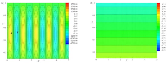
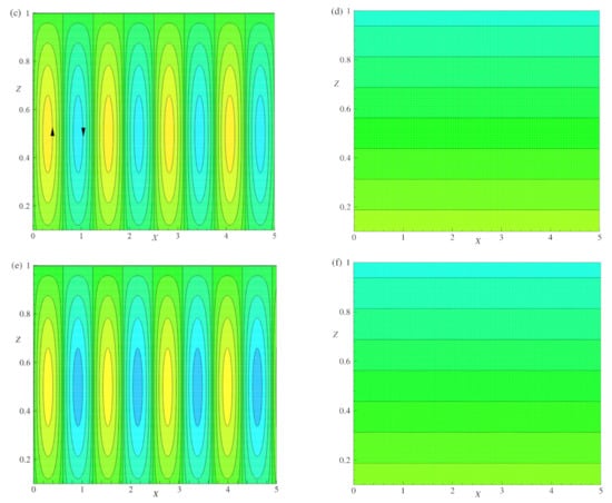
Figure 5. The Effect of E and $\mathsf{\Lambda }$ near $R_{cs}$, streamlines (a) for E = 0.005, $\mathsf{\Lambda }$ = 0.2, and $q=0.01$, (c) E = 0.01, $\mathsf{\Lambda }$ = 0.2, and $q=0.01$, (e) E = 0.005, $\mathsf{\Lambda }$ = 0.4, and $q=0.01$ and isotherms (b) E = 0.005, $\mathsf{\Lambda }$ = 0.2, and $q=0.01$, (d) E = 0.01, $\mathsf{\Lambda }$ = 0.2, and $q=0.01$, (f) E = 0.005, $\mathsf{\Lambda }$ = 0.4, and $q=0.01$ are plotted.

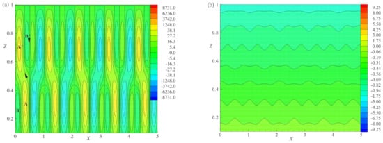
Figure 6. The Effect of R = 10$R_{cs}$, $20R_{cs}$, $30R_{cs}$ and $80R_{cs}$, streamlines (a,c,e,g) and isotherms (b,d, f, h) are plotted for E = 0.005, $\mathsf{\Lambda }$ = 0.2, and q = 0.01.

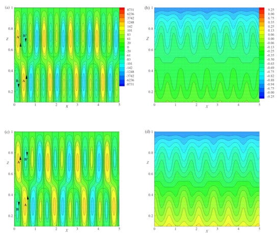
Figure 7. The Effect of E = 0.01 and 0.015, streamlines (a,c) and isotherms (b,d) are plotted for $\mathsf{\Lambda }$ = 0.2, R = 20$R_{cs}$, and $q=0.01$.

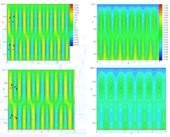
Figure 8. The Effect of $\mathsf{\Lambda }$ = 0.4 and 0.6, streamlines (a,c) and isotherms (b,d) are plotted for E = 0.005, R = $20R_{cs}$ and q = 0.01.

The snapshot of streamlines and isotherms for different values of R and for fixed values of $E=0.005$, $\mathsf{\Lambda }=0.2$, and $q=0.01$ are displayed in Figure 6a–h. It is observed that for $R=10R_{cs}$ and for the cell lying between $0\le X\le 1$, the absolute minimum and maximum values are with the circulation strengths $-43.4965$ and $43.4965$, respectively, as shown in Figure 6a. As R increases from $R_{cs}$ to $10R_{cs}$, the basic cells become more deformed due to the growth of two vortices B and $B^{\prime }$ located at the top right and bottom left boundaries with the circulation strength $-16.315$. The basic cell with two vortices A and $A^{\prime }$ has circulation strength $38.059$. The temperature profiles in terms of isotherms are illustrated in Figure 6b for same values of physical parameters that are considered in Figure 6a. The isotherms are of nearly in wavy shape with the absolute maximum and minimum values of $-0.00212$ and $-1.00271$, respectively. It indicates the maximum of heat transfer process is occurred by convection. Figure 6c,d illustrate the streamlines and isotherms for $R=20R_{cs}$. The temperature gradient and the gravitational buoyancy force act together and changes the flow structure as shown in Figure 6c. The bicellular patterns of streamlines turn out to be multicellular models and these cells divide the field of motion at the core for a cell lies between $0\le X\le 1$ with the absolute maximum and minimum values of circulation strengths $220.829$ and $-220.845$, respectively. The vortices B and $B^{\prime }$ showed their presence with $-82.822$ as the circulation strength in the opposite direction of an original cell. For these considered values of physical parameters, the behavior of isotherms is shown in Figure 6d, which exhibit the mode of convective heat transport inside the fluid layer. In the fluid layer, the absolute maximum and minimum values of isotherms are respectively, $-0.00275$ and $-1.0052$. When R is increased from $20R_{cs}$ to $30R_{cs}$, the small vortices B and $B^{\prime }$ shown in Figure 6c are increased with circulation strength $-398.740$. Thus, the basic cell encountered more deformation (Figure 6e) and has the absolute maximum and minimum values at $638.172$ and $-638.027$, respectively. Accordingly, the isotherm curves develop more deformation. The absolute maximum and minimum values of isotherms in the layer are, respectively, $-0.00449$ and $-1.01101$. As R is increased from $30R_{cs}$ to $80R_{cs}$ (Figure 6g), the two vortices B and $B^{\prime }$ grow in size and split the basic cell into two vortices located on either side of the secondary cell with the absolute maximum ($9976.78$) and minimum ($-9977.74$) strengths. The heat flow pattern becomes chaotic, which is shown in Figure 6h when R increases to $80R_{cs}$. The absolute maximum and minimum values of isotherms in the layer are, respectively, $8.75285$ and $-9.67347$. From Figure 6, it is observed that as R increases from $R_{cs}$ to $80R_{cs}$, the onset of turbulent flows are producible.

Figure 7a–d, illustrate the streamlines and isotherms for different values of E and for a fixed set of other parameters $R=20R_{cs}$, $\mathsf{\Lambda }=0.2$, and $q=0.01$. The behavior of the flow field was investigated by considering the flow pattern in the region $0\le X\le 1$, as shown in Figure 6a–d (E = $0.005$) and Figure 7a–d (E = $0.01$ and $0.015$). Figure 7a shows streamlines for E = $0.01$ in the considered range of X. The absolute maximum and minimum values of circulation strengths are $162.15$ and $-162.149$, respectively. There exist two vortices B and $B^{\prime }$ outside the basic cell with the circulation strength $-82.806$ as shown in Figure 7a. The basic cell also contains two vortices namely A and $A^{\prime }$ with a circulation strength of $141.881$. Figure 7c is plotted for E = $0.015$, which has the absolute maximum and absolute minimum values of circulation strength as $140.453$ and $-140.471$, respectively. The flow pattern in the region $0\le X\le 1$ contains a deformed basic cell due to the growth of two vortices B and $B^{\prime }$ that exist at either side of the basic cell and are located at the top and bottom boundaries with circulation strength $-60.81$. The basic cell also has two vortices A and $A^{\prime }$ with a circulation strength value of $122.90$. Finally from Figure 6c and Figure 7a,c it is observed that the strength of the basic cell and pattern deformation decrease as E increases. This implies that the effect of E stabilizes the convective system. The flow of heat transfer is shown in Figure 7b,d for E = $0.01$ and $0.015$, respectively.

Figure 8a–d show the streamlines and isotherms for different $\mathsf{\Lambda }$ values and for $E=0.005$, $R=20R_{cs}$, and $q=0.01$. The effect of $\mathsf{\Lambda }$ was studied from Figure 6c,d and Figure 8a–d. In Figure 8a the streamlines are plotted for $\mathsf{\Lambda }=0.4$. By considering the flow pattern in the range of $0\le X\le 1$, the absolute maximum and minimum values of circulation strengths are $436.721$ and $-436.747$, respectively. In this range, the basic cell is deformed by two vortices B and $B^{\prime }$, which are located at the top right and bottom left of the layer and on either side of the basic cell with circulation strength $-272.97$. The basic cell also encloses two vortices A and $A^{\prime }$ with strength $382.13$. Figure 8c shows the streamlines for $\mathsf{\Lambda }=0.6$ in the considered range of $0\le X\le 1$, with the absolute maximum and minimum values of circulation strength $663.595$ and $-663.555$, respectively. In addition, there exist two vortices B and $B^{\prime }$ with circulation strength $-414.71$. The basic cell also enclosed two vortices A and $A^{\prime }$ with circulation strength $580.65$. As $\mathsf{\Lambda }$ increases from $0.4$ to $0.6$ the deformation and circulation strength of cells ($A,A^{\prime }$) increase. This implies that the effect of $\mathsf{\Lambda }$ destabilizes the convective system. The isotherms are plotted in Figure 6d and Figure 8b,d for distinct values of $\mathsf{\Lambda }=0.2,0.4$ and $0.6$. The lines of isotherms change to a more circular form as $\mathsf{\Lambda }$ increases. Thus, the incremental values of $\mathsf{\Lambda }$ destabilize the convective system.

Topology of Flow

The topology constraint is based on the Euler number (${\zeta }^{{}^{\prime }}$) of the flow. As described by Jana et al. [27], ${\zeta }^{{}^{\prime }}$ on the surface is defined as the sum of the Poincare indices of the critical points on the surface and is given by

$$\begin{array}{c}\hfill NE-(NH+\frac{1}{2}NP)={\zeta }^{{}^{\prime }},\end{array}$$

(70)

here the $NE$ represents the number of elliptic points, $NH$ is the number of hyperbolic points, and $NP$ is the number of parabolic points [28,29]. In Figure 9a, the vorticity contours are exhibited for $R\simeq R_{cs}$, E= 0.005, $\mathsf{\Lambda }$= 0.2 and $q=0.01$. The present simulated flow fulfils the topological rule given in Equation (70) with $NP=0$ , $NH=2$, and $NE=2$. For $R=20R_{cs}$, an equivalent investigation has been done for vorticity contours in Figure 9b and Equation (70) is satisfied with $NP$ = 0, $NE$ = 8, and $NH$ = 8.

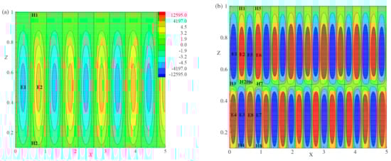
Figure 9. Vorticity lines for (a) $R\simeq R_{cs}$, E = 0.005, $\mathsf{\Lambda }$ = 0.2, and $q=0.01$, (b) R = 20$R_{cs}$, E = 0.005, $\mathsf{\Lambda }$ = 0.2, and $q=0.01$.

7. Heat Function

Heatlines depict the convective heat transport phenomenon, whereas the isotherms are mainly useful for visualizing heat transfer in the domain of conduction. The heat function and heatline analyzes were developed by Kimura and Bejan [30] to visualize heat transmission through the fluid flow, later Morega and Bejan [31] successfully used the concept of heatlines. Different researchers [32,33,34,35] used this concept for dissimilar applications of natural convective systems. The heat function ($H^{*}$) is defined as

$$\begin{array}{c}\hfill \frac{\partial H^{*}}{\partial X}=WT-\frac{\partial T}{\partial Z},\end{array}$$

(71)

$$\begin{array}{c}\hfill -\frac{\partial H^{*}}{\partial Z}=UT-\frac{\partial T}{\partial X},\end{array}$$

(72)

where $T=T_s+\theta$ and $T_s=T_0-Z$. The Equations (71) and (72) do not exhibit the symmetric property. Differentiating Equations (71) and (72) with respect to X and Z, respectively, and subtracting the resulting equations yields

$$\begin{array}{c}\hfill \frac{{\partial }^2{H}^{*}}{\partial X^2}+\frac{{\partial }^2{H}^{*}}{\partial Z^2}=\frac{\partial \left(WT\right)}{\partial X}-\frac{\partial \left(UT\right)}{\partial Z}.\end{array}$$

(73)

From the definition of heat function, Equations (71) and (72), the boundary conditions on $H^{*}$ follow [16]:

$$\begin{array}{c}\hfill H^{*}(X,0)=H^{*}(0,0)+{\int }_0^X(WT-\frac{\partial T}{\partial Z})dX,\mathrm{at}Z=0\mathrm{and}0\le X\le \sqrt{2}\pi /a,\end{array}$$

(74)

$$\begin{array}{c}\hfill H^{*}(X,1)=H^{*}(0,1)+{\int }_0^X(WT-\frac{\partial T}{\partial Z})dX,\mathrm{at}Z=1\mathrm{and}0\le X\le \sqrt{2}\pi /a,\end{array}$$

(75)

$$\begin{array}{c}\hfill H^{*}(0,Z)=H^{*}(0,0)-{\int }_0^Z(UT-\frac{\partial T}{\partial Z})dZ,\mathrm{at}X=0\mathrm{and}0\le Z\le 1,\end{array}$$

(76)

$$\begin{array}{c}\hfill H^{*}(\sqrt{2}\pi /a,Z)=H^{*}(\sqrt{2}\pi /a,0)-{\int }_0^Z(UT-\frac{\partial T}{\partial Z})dZ,\mathrm{at}X=\sqrt{2}\pi /a\mathrm{and}0\le Z\le 1.\end{array}$$

(77)

Results and Discussion for Heatlines

Figure 10a–d, illustrate the pattern of heatlines for different Rayleigh number values, $R\simeq R_{cs}$, $R=$$1.05R_{cs}$, $1.15R_{cs}$ and $1.25R_{cs}$, respectively, for fixed values of $E=0.005$, $\mathsf{\Lambda }=0.2$, and $q=0.01$. When the system is at a conduction state ($R<R_{cs}$) heatlines are always parallel to Z-axis and perpendicular to isotherms. Figure 10a illustrates the heatlines for $R\simeq R_{cs}$. It is observed that the heatline contours within the domain are normal to the $Z=0$ and $Z=1$ lines due to conduction dominant heat transfer. For $R\simeq R_{cs}$, the absolute maximum and minimum values of heatlines are $10.2224$ and $0.0241$, respectively, in the considered range $0\le X\le 5$. In the neighborhood of $X=0$, the heatlines at the center of the system depict the structure which is similar to the parabolic structure. The curvature at the central part of the system increases as X increases. This shows that the nonlinear propagation of heat transfer occurs when $R\simeq R_{cs}$. Hence, the transition takes place from the conduction state to the convection state at $R\simeq R_{cs}$. Figure 10b is plotted for $R=1.05R_{cs}$. The absolute maximum and minimum values of heatlines are $10.3081$ and $-0.2774$, respectively, in the considered range $0\le X\le 5$. The heatline with a strength of $-0.18$ exist near the line $X=0$ and the heatline with strength $9.69$ exist at $X=5$. The strength of heatlines increases as X increases. Some heatlines occurred in the form of a closed path. As R increases from $R_{cs}$ the heatlines with same strength are changed to a closed path as shown in Figure 10a,b. For higher values, this indicates that the convective heat flow is more intense at the center. Figure 10c shows heatlines at $R=1.15R_{cs}$ and having the absolute maximum and minimum values of heatlines $10.3666$ and $-0.62655$, respectively. In this figure, the number of closed paths of heatlines at the center is increased for $R=1.15R_{cs}$. The size of closed path of heatlines for $R=1.15R_{cs}$ is more than that for $R=1.05R_{cs}$. Figure 10d shows the heatlines for $R=1.25R_{cs}$ with the absolute maximum and minimum values of $10.3972$ and $-0.88096$, respectively. The number of closed paths of heatlines increases at the center for $R=1.25R_{cs}$. The size of closed path of heatlines for $R=1.25R_{cs}$ is increased in comparison with that of the heatlines for $R=1.15R_{cs}$. For large R, the convective heat transmission is more intense. It is observed that the heatlines become denser with the increase in R. Figure 10a–d indicate that the heat transfer across the layer is increased as R increases. Heatlines will not exhibit periodic patterns due to the non-symmetry nature of Equations (71) and (72).

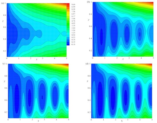
Figure 10. The effect of $R\simeq R_{cs}$, R = 1.05$R_{cs}$, 1.15$R_{cs}$ and $1.25R_{cs}$, heatlines (a–d) are plotted for E = 0.005, $\mathsf{\Lambda }$ = 0.2, $T_0$ = 1, and q = 0.01, respectively.

Figure 10b and Figure 11a,b are plotted with the same strength of heatlines so as to analyze the influence of E on heat flow for the fixed values of $\mathsf{\Lambda }$, R, and q. In the considered range of $0\le X\le 5$, for $E=0.01$, (Figure 11a) the absolute maximum and minimum values of heatlines are noted to be $8.4264$ and $-0.18554$, respectively, and for $E=0.015$ (Figure 11b) these values are $7.51142$ and $-0.11574$, respectively. In both of these Figure 11a,b, the heatlines intensity decays with E. The size of the closed path and the number of closed paths with the same strength decreased as E increases. From Figure 10b and Figure 11a,b it is fascinating to observe the inhibition of temperature in the central regime as E increases.

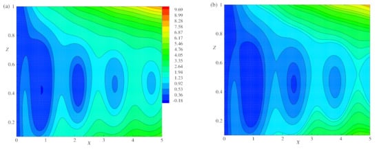
Figure 11. The effect of E = 0.01 and 0.015, heatlines (a,b) are plotted for $\mathsf{\Lambda }$ = 0.2, R = 1.05$R_{cs}$, $T_0$ = 1, and $q=0.01$.

Figure 10b and Figure 12a,b are plotted with the same strength of heatlines to analyze the effect of $\mathsf{\Lambda }$ on heat flow for the fixed values of E, R, and q. In the considered range of $0\le X\le 5$ for $\mathsf{\Lambda }=0.4$ (Figure 12a) with the absolute maximum and minimum values of heatlines as $8.55642$ and $-0.23723$, respectively. These values for $\mathsf{\Lambda }=0.6$ (Figure 12b) are $7.74043$ and $-0.18296$, respectively. In both Figure 12a,b, the heatlines are dominated by convection and form closed loops. The size and the number of closed loops with the same strength increase as $\mathsf{\Lambda }$ increases. From Figure 10b and Figure 12a,b it is observed that the temperature within the central regime is enhanced as $\mathsf{\Lambda }$ increase by observing heatlines.

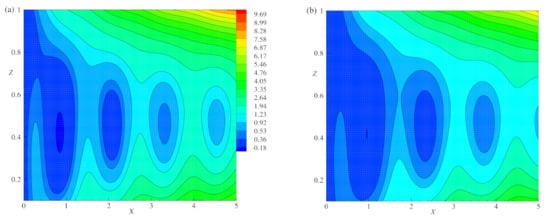
Figure 12. The effect of $\mathsf{\Lambda }$ = 0.4 and 0.6, heatlines (a,b) are plotted for E = 0.005, R = 1.05 $R_{cs}$, $T_0$ = 1, and $q=0.01$.

8. Conclusions

The nonlinear natural convection was studied in a planer layer of electrically conducting fluid that rotates about the vertical axis in the presence of a uniform horizontal magnetic field and vertical temperature gradient. This problem has applications in Earth’s liquid core. The present results help to enhance understanding of the finite amplitude convection when the coupling between the Lorentz force and the Coriolis force present in nonlinear planar layer convection-driven dynamos.

• Linear stability analysis showed that as the small values of E keep decreasing or $\mathsf{\Lambda }$ increasing, the $R_{cs}$ decreases, i.e., the effect of E stabilizes and $\mathsf{\Lambda }$ destabilizes the system.
• Theoretically investigated the nonlinear behavior of cross rolls that occur in the Rayleigh–Bénard convective system of a planar layer dynamo of electrically conducting fluid rotating about the vertical axis in the presence of a horizontal magnetic field.
• The nonlinear partial differential equations was solved using the perturbation method, until $O\left({ϵ}^8\right)$ and obtained the approximate solutions.
• Computed the local Nusselt number ($N_L$) and averaged Nusselt number ($Nu$) on the hot wall to understand the development of heat flow and the rate of heat transfer, respectively.
• The number of peaks is fixed for a given E while the value of the peak is independent of X for a given E. The absolute peak values of $N_L$ increase as E increases. The number of peaks is fixed for a given $\mathsf{\Lambda }$. The value of the peak is independent of X for a given $\mathsf{\Lambda }$. The absolute peak value of $N_L$ increases as $\mathsf{\Lambda }$ decrease. From the $N_L$ results, it is noted that the heat flux is high for decreasing E or increasing $\mathsf{\Lambda }$.
• It is observed that the Ekman number (E) generates a strong damping effect on heat transfer at high rotation rates but the heat transport enhances as $\mathsf{\Lambda }$ increases. The Roberts number (q) < 1, enhances the heat transfer rate and accordingly the intensity of the flow rate also increases. Similarly, the total energy decays as E increases. The increment in the values of $\mathsf{\Lambda }$ show, the increase in the total energy.
• Obtained the cellular pattern of fluid flow (streamlines) and the hot regions (isotherms) from the eigenfunctions related to the stream function and temperature, respectively. From the streamlines and isotherms trajectories, it is observed that, for the lower values of E the deformation of the fluid pattern is enhanced and more transfer of heat in the flow occurs due to the presence of lesser viscous force in comparison with the Coriolis force. Similarly, for the amplifying values of $\mathsf{\Lambda }$, there is more deformation in the streamlines and isotherms. This result shows, in the presence of Coriolis force, the magnetic field destabilizes the system.
• Studied the heatline patterns of the flow by using the heat function. The results show that the deformation in the trajectories of heatlines are enhanced as E decreases. A similar trend of deforming heatlines is observed with increasing $\mathsf{\Lambda }$.

References

- Chandrasekar, S. Hydrodynamic and Hydromagnetic Stability; Oxford Clarendon Press: Oxford, UK, 1961. [Google Scholar]
- Robert, P.H. An Introduction to Magnetohydrodynamics; American Elsevier: New York, NY, USA, 1967. [Google Scholar]
- Cox, S.M.; Mathews, P.C. New instabilities in two-dimensional rotating convection and magnetoconvection. Phys. D 2001, 149, 210. [Google Scholar] [CrossRef]
- Malkus, W.V.R.; Veronis, G. Finite Amplitude Cellular Convection. J. Fluid Mech. 1958, 4, 225–260. [Google Scholar] [CrossRef]
- Kuo, H.L. Solution of the non-linear equations of the cellular convection and heat transport. J. Fluid Mech. 1960, 10, 611–630. [Google Scholar] [CrossRef]
- Braginsky, S.I. Magnetohydrodynamics of the Earth’s core. Geomagn. Aeron. 1964, 4, 698–712. [Google Scholar]
- Eltayeb, I.A. Hydromagnetic convection in a rapidly rotating fluid layer. Proc. R. Soc. Lond. A 1972, 326, 229–254. [Google Scholar]
- Eltayeb, I.A. Overstable hydromagnetic convection in a rotating fluid layer. J. Fluid Mech. 1975, 71, 161–179. [Google Scholar] [CrossRef]
- Aurnou, J.M.; Olson, P.L. Experiments on Rayleigh–Bénard convection, magnetoconvection and rotating magnetoconvection in liquid gallium. J. Fluid Mech. 2000, 430, 283–307. [Google Scholar] [CrossRef]
- Raju, C.S.K.; Ameer Ahammad, N.; Sajjan, K.; Shah, N.A.; Yook, S.; Dinesh Kumar, M. Nonlinear movements of axisymmetric ternary hybrid nanofluids in a thermally radiated expanding or contracting permeable Darcy Walls with different shapes and densities: Simple linear regression. Int. Commun. Heat Mass Trans. 2022, 135, 106110. [Google Scholar] [CrossRef]
- Kumar, M.D.; Raju, C.S.K.; Sajjan, K.; El-Zahar, E.R.; Shah, N.A. Linear and quadratic convection on 3D flow with transpiration and hybrid nanoparticles. Int. Commun. Heat Mass Trans. 2022, 134, 105995. [Google Scholar] [CrossRef]
- Rani, H.P.; Rameshwar, Y.; Brestensky, J. Topology of Rayleigh-Bénard convection and magnetoconvection in plane layer. Geophys. Astrophys. Fluid Dyn. 2019, 113, 208–221. [Google Scholar] [CrossRef]
- Roberts, P.H.; Jones, C.A. The onset of magnetoconvection at large Prandtl number in a rotating layer 1. Finite magnetic diffusion. Geophys. Astrophys. Fluid Dyn. 2000, 92, 289–325. [Google Scholar] [CrossRef]
- Braginsky, S.I. Torsional magnetohydrodynamic vibrations in the Earth’s core and variations in the day length. Geomagn. Aeron. 1970, 10, 3–12. [Google Scholar]
- Robert, P.H.; Stewartson, K. On Finite Amplitude Convection in a Rotaiting Magnetic System. Philos. Trans. R. Soc. Lond. Ser. Math. Phys. Sci. 1974, 277, 287–315. [Google Scholar]
- Rameshwar, Y.; Rawoof Sayeed, M.A.; Rani, H.P.; Laroze, D. Finite amplitude cellular convection under the influence of a vertical magnetic field. Int. J. Heat Mass Transf. 2017, 114, 559–577. [Google Scholar] [CrossRef]
- Rawoof Sayeed, M.A.; Rameshwar, Y. Finite Amplitude Cellular Thermohaline Convection. J. Heat Transf. 2022, 114, 112602. [Google Scholar] [CrossRef]
- Rameshwar, Y.; Srinivas, G.; Laroze, D.; Rawoof Sayeed, M.A.; Rani, H.P. Convective instabilities in binary mixture 3He-4He in porous media. Chin. J. Phys. 2022, 77, 773–803. [Google Scholar] [CrossRef]
- Rameshwar, Y.; Srinivas, G.; Laroze, D. Finite amplitude oscillatory convection of binary mixture kept in a porous medium. Processes 2023, 11, 664. [Google Scholar] [CrossRef]
- Baklouti, F.S.; Khlifi, A.; Salhi, A.; Godeferd, F.; Cambon, C.; Lehner, T. Kinetic-magnetic energy exchanges in rotating magnetohydrodynamic turbulence. J. Turbul. 2019, 20, 263–284. [Google Scholar] [CrossRef]
- Gupta, V.K.; Keshri, O.P.; Kumar, A. Effect of rotational speed modulation on weakly nonlinear magneto convective heat transfer with temperature-dependent viscosity. Chin. J. Phys. 2021, 72, 487–498. [Google Scholar] [CrossRef]
- Jones, C.A.; Roberts, P.H. The onset of magnetoconvection at large Prandtl number in a rotating layer. II. Small magnetic diffusion. Geophys. Astrophys. Fluid Dyn. 2000, 93, 173–226. [Google Scholar] [CrossRef]
- Šoltis, T.; Brestenský, J. Rotating magnetoconvection with anisotropic diffusivities in the Earth’s core. Phys. Earth Planet. Int. 2010, 178, 27–38. [Google Scholar]
- Filippi, E.; Brestenský, J.; Šoltis, T. Effects of anisotropic diffusion on onset of rotating magnetoconvection in plane layer; stationary modes. Geophys. Astrophys. Fluid Dyn. 2019, 113, 80–106. [Google Scholar] [CrossRef]
- Sparrow, E.M.; Carlson, C.K. Local and average natural convection Nusselt numbers for a uniformly heated, shrouded or unshrouded horizontal plate. Int. J. Heat Mass Transf. 1986, 29, 369–379. [Google Scholar] [CrossRef]
- Batchelor, G.K. An Introduction to Fluid Dynamics; Cambridge University Press: Cambridge, UK, 1993. [Google Scholar]
- Jana, S.C.; Metcalfe, G.; Ottino, J.M. Experimental and computational studies of mixing in complex Stokes flows: The vortex mixing flow and multicellular cavity flows. J. Fluid Mech. 1994, 269, 199–249. [Google Scholar] [CrossRef]
- Tony Sheu, W.H.; Rani, H.P. Exploration of vortex dynamics for transitional flows in a three-dimensional backward facing step channel. J. Fluid Mech. 2006, 550, 61–83. [Google Scholar] [CrossRef]
- Sheu, T.; Rani, H.P.; Ten-China, T.; Tsai, S.F. Multilple states, topology and bifurcations of natural convection in a cubical cavity. Comput. Fluids 2008, 37, 1011–1028. [Google Scholar] [CrossRef]
- Kimura, S.; Bejan, A. The heatline visualization of convective heat transfer. J. Heat Transf. 1983, 105, 916–919. [Google Scholar] [CrossRef]
- Morega, A.I.; Bejan, A. Heatline visualization of forced convection laminar boundry layers. Int. J. Heat Mass Transf. 1993, 36, 3957–3966. [Google Scholar] [CrossRef]
- Bejan, A. Convection Heat Transfer; Wiley: New York, NY, USA, 1984; pp. 21–23. [Google Scholar]
- Komori, K.; Kito, S.; Naumara, T.; Inaguma, Y.; Inagai, T. Fluid flow and heat transfer in the transition process of natural convection over an inclined plate. Heat Trans. Asian Res. 2001, 30, 648–659. [Google Scholar] [CrossRef]
- Kimura, F.; Kitamura, K.; Yamaguchi, M.; Asami, T. Fluid flow and heat transfer of natural convection adjacent to upward facing inclined heated plates. Heat Trans. Asian Res. 2003, 32, 278–291. [Google Scholar] [CrossRef]
- Hooman, K.; Gurgechi, H.; Dincer, I. Heatline and energy-flux-vector visualization of natural convection in a porous cavity occupied by a fluid with temperature-dependent viscosity. J. Porous Media 2009, 12, 265–275. [Google Scholar] [CrossRef]
Disclaimer/Publisher’s Note: The statements, opinions and data contained in all publications are solely those of the individual author(s) and contributor(s) and not of MDPI and/or the editor(s). MDPI and/or the editor(s) disclaim responsibility for any injury to people or property resulting from any ideas, methods, instructions or products referred to in the content. |
© 2023 by the authors. Licensee MDPI, Basel, Switzerland. This article is an open access article distributed under the terms and conditions of the Creative Commons Attribution (CC BY) license (https://creativecommons.org/licenses/by/4.0/).