Dynamics of a Two Prey and One Predator System with Indirect Effect

Abstract

We study a population model with two preys and one predator, considering a Holling type II functional response for the interaction between first prey and predator and taking into account indirect effect of predation. We perform the stability analysis of equilibria and study the possibility of Hopf bifurcation. We also include a detailed discussion on the problem of persistence. Several numerical simulations are provided in order to illustrate the theoretical results of the paper.

1. Introduction

Population dynamics has been extensively studied by researchers in biomathematics, particularly the predator–prey models.

In [1], the authors consider the following two prey one predator model:

$$\begin{array}{cc}\hfill & \dot{x}=rx\left(1-\frac{x}{k}\right)-\frac{cxz}{a+\alpha \eta y+x},\hfill \\ \hfill & \dot{y}=y(\beta -\delta z),\hfill \\ \hfill & \dot{z}=\frac{bxz}{a+\alpha \eta y+x}+\gamma yz-mz,\hfill \end{array}$$

(1)

where $x,y,z$ represent the population densities of the two preys and of the predator, respectively.

In the previous model, for the interaction between the first prey and the predator, they considered a Holling type II functional response where the handling time of predator for the second prey is also involved, whereas for the interaction between the second prey and the predator, they considered a Lotka–Volterra functional response. It is also assumed that there is no intraspecific interaction in the second prey population and its growth is exponential; as a consequence, there is a huge availability of second prey in the absence of a predator, and there is no searching time for the second prey population. They found necessary and sufficient conditions for existence and stability of the nontrivial equilibrium $E^{*}$ (see [1]).

In order to recover a more complex behavior, we consider a modification of the model that takes the indirect effects of predations into account.

The role played by indirect effects in population dynamics has been investigated in the last several decades (see [2,3,4,5,6,7,8,9,10,11,12]). In the case of predation, it has been pointed out (see [13]) that predator can alter the morphology (see [6]) or the behavior of the preys. In particular, the preys, in order to avoid contacts with predators, may reduce their normal activity or may stay hidden most of the time. Many kinds of indirect effects have been described in the literature (see, for example, [8] for a detailed discussion); an interesting example (see [14]) is the case of refuge indirect effect.

A model was proposed in order to take into account indirect interactions in a plankton community (see [15] and the references quoted therein). They analyzed the effects of predator Daphnia over two groups of phytoplankton of different morphology (see [7,9]), having phosphorous as a resource (see [5,9]). In this case, the predator prefers to predate the smaller size prey group and the other one take advantages of it.

The model was analytically studied in [15] using persistence theory (see [16,17]) and in [18] using bifurcation theory. Both studies suggest the importance of indirect effects of predation in order to describe cases of coexistence in real life. In [19], seasonal indirect effects were considered to show the possibility of chaotic motion, whereas in [20,21], the authors considered the stochastic version of the model. Regarding the model (1), since there is a higher availability of the second prey, it is natural to suppose that the predator prefer to predate the second prey and the first one take advantages of it. The easiest way to model this situation consists of adding the indirect effect term $-Lyz$ in the second equation and the term $Lyz$ in the first one, with the parameter $L>0$ describing the intensity of indirect effects. The systems become

$$\begin{array}{cc}\hfill & \dot{x}=rx\left(1-\frac{x}{k}\right)-\frac{cxz}{a+\alpha \eta y+x}+Lyz,\hfill \\ \hfill & \dot{y}=y(\beta -\delta z)-Lyz,\hfill \\ \hfill & \dot{z}=\frac{bxz}{a+\alpha \eta y+x}+\gamma yz-mz.\hfill \end{array}$$

(2)

We will consider initial conditions $x\left(0\right)\ge 0$, $y\left(0\right)\ge 0$, $z\left(0\right)\ge 0$ and we assume all the parameters are positive and with the following meaning: r and k are the intrinsic growth rate and carrying capacity of the first prey, respectively; $\beta$ and $\delta$ are the intrinsic growth rate and predation rate of the second prey, respectively; a is the half saturation value of the predator; b is the maximum growth rate of the predator; c is the maximum rate of predation for first prey item; m is the death rate of the predator in the absence of prey; $\alpha$ is the quotient of the handling time of the predator per second prey item and the handling time of the predator per first prey item; $\eta$ is the quotient of the capture rate of the second prey and the capture rate of the first prey; $\gamma$ is the efficiency with which the second prey consumed by the predator gets converted into predator biomass (see [1] for more details).

We note that the system is not of Kolmogorov type; indeed, the first equation cannot be written in the form

$$\dot{x}=xf(x,y,z).$$

Such systems can be regarded as semi-Kolmogorov systems using a terminology introduced in [19].

For system (2), we perform the stability analysis of equilibria and we analyze the existence of limit cycles by Hopf bifurcation, as they play an important role in the qualitative theory of differential systems. The study of limit cycles was initiated by Poincaré [22] and motivated by the famous 16th Hilbert problem [23,24,25] and by the fact that the behavior of many natural phenomena has been modelized by limit cycles, as, for instance, the famous limit cycle of van der Pol [26].

In the last several decades, the existence of limit cycles for systems with biological meaning, such as the Lotka–Volterra or Kolmogorov system, have been studied through Hopf and zero-Hopf bifurcation (see, for example, [27,28] for recent results).

The rest of the paper is organised as follows: in Section 2, we present a preliminary analysis of the features of the model. In Section 3 we provide a study of existence and stability of equilibria. In Section 4, we discuss the problem of persistence of the three species. In Section 5, we present a case of Hopf bifurcation. Finally, Section 6 contains some conclusive remarks.

2. Analysis of the System (2) on the Invariant Planes

First, we will show that the dynamics of the system, considering positive initial conditions, is contained in the first octant.

Theorem 1.

The set $\{(x,y,z)\in {\mathbb{R}}^3:x,y,z\ge 0\}$ is positively invariant for system (2).

Proof. 

At first, we must note that the planes $z=0$ and $y=0$ are invariant. On the plane $x=0$, we have $\dot{x}=Lyz>0$; then, solutions do not leave the positive octant, that is, the set $\left\{\right(x,y,z)\in \mathbb{R}:x,y,z\ge 0\}$ is positively invariant. □

We analyze the dynamics on the boundary of $\left\{\right(x,y,z)\in \mathbb{R}:x,y,z\ge 0\}$. In order to do that, we first study the dynamics on the coordinate axes and then on the planes $y=0$ and $z=0$.

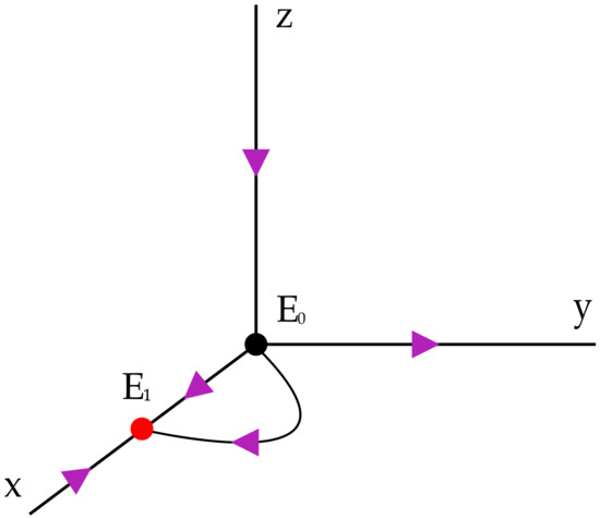
The three axes are invariant for the dynamics; in particular, any solution with initial conditions on the x-axis tends to the equilibrium $(k,0,0)$, any solution with initial conditions on the z-axis tends to the equilibrium $(0,0,0)$, and any solution with initial conditions on the y-axis verifies that $y\left(t\right)$ tends to infinity when t tends to infinity. See Figure 1.

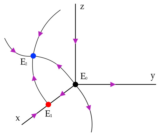
Figure 1. The dynamics on the axes.

Now, we present some considerations about the dynamics on the invariant planes. On the invariant plane, $z=0$ the system is

$$\begin{array}{cc}\hfill & \dot{x}=rx\left(1-\frac{x}{k}\right),\hfill \\ \hfill & \dot{y}=\beta y,\hfill \end{array}$$

(3)

and for this system, solutions are unbounded except that on the positive x-axis. The equilibrium points are $(0,0)$ and $(k,0)$. The eigenvalues of $DF(0,0)$ are r and $\beta$, which are both positive, so this equilibrium is an unstable node. The eigenvalues of $DF(k,0)$ are $-r$ and $\beta$, so the equilibrium point is a saddle.

On the plane $y=0$, the system is

$$\begin{array}{cc}\hfill & \dot{x}=rx\left(1-\frac{x}{k}\right)-\frac{cxz}{a+x},\hfill \\ \hfill & \dot{z}=\frac{bxz}{a+x}-mz,\hfill \end{array}$$

(4)

and the equilibria are $(0,0)$, $(k,0)$. If

$$kb>m(k+a)$$

there exists a further equilibrium point with coordinates $(m/(b-m),\overline{z})$ where

$$\overline{z}=\frac{r}{c}\left(\frac{ba}{b-m}\right)\left(1-\frac{ma}{k(b-m)}\right).$$

The eigenvalues of $DF(0,0)$ are r and $-m$, so it is a saddle. The eigenvalues of $DF(k,0)$ are $-r$ and $bk/(a+k)-m$. The first one is negative and the second changes it sign when $bk=(a+k)m$. When $bk/(a+k)-m<0$, it is a stable node, and when $bk/(a+k)-m>0$, it loses its stability; it becomes a saddle and the third equilibrium appears.

The x-nullclines are $x=0$ and $z=(r/(ck\left)\right)(k-x)(a+x)$. If $bk/(a+k)=m$, then $\dot{z}=\left(ba(x-k)\right)/\left((a+x)(a+k)\right)z$ is positive if $x>k$ and negative if $x<k$. The local phase portrait in this case is given in Figure 2.

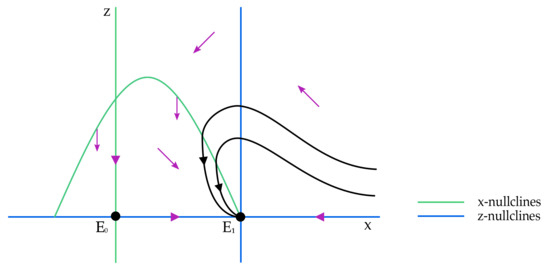
Figure 2. Phase portrait on the plane $y=0$ with $bk/(a+k)=m$.

When $bk/(a+k)>m$, the equilibrium $(ma/(b-m),\overline{z})$ appears, as is it shown in Figure 3. The eigenvalues of the Jacobian matrix of system (4) at $E_2$ are

$${\lambda }_{1,2}={\displaystyle \frac{A_1\pm \sqrt{A_2}}{A_3}},$$

(5)

where

$$\begin{array}{cc}\hfill A_1& =-cmr\left(k(m-b)+a(m+b)\right),\hfill \\ \hfill A_2& =c^{2}mr\left(4bk{(b-m)}^2(m(a+k)-bk)+mr{\left(k(m-b)+a(m+b)\right)}^2\right),\hfill \\ \hfill A_3& =2bck(b-m).\hfill \end{array}$$

(6)

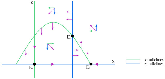
Figure 3. Phase portrait on the plane $y=0$ with $bk/(a+k)>m$.

Note that $A_3>0$ by the existence conditions of the equilibrium point. These eigenvalues are complex if $A_2<0$, and in that case, they have a positive real part if

$$m<\frac{b(k-a)}{k+a},$$

(7)

in which case, $E_2$ is unstable. If

$$m>\frac{b(k-a)}{k+a},$$

(8)

the real part of the eigenvalues is negative, so $E_2$ is asymptotically stable. In the case with $A_2>0$, as the determinant of the Jacobian matrix is positive, it is not possible that the eigenvalues have different sign. Then, if $A_1$ is positive, both eigenvalues are positive and $E_2$ is unstable. In other case, from the conditions $A_1+\sqrt{A_2}<0$ and $A_1-\sqrt{A_2}<0$ we would get that $A_1<-\sqrt{A_2}<0$, which is a contradiction. In the same way, we obtain that if $A_1<0$, then both eigenvalues are negative and $E_2$ is asymptotically stable.

We give here some results about the possible existence of periodic orbits surrounding the equilibrium point $E_2$ in the plane $y=0$.

The equilibrium point $E_2$ is a Hopf equilibrium if and only if $A_1=0$ and $A_2<0$, it is, when $m=b(k-a)/(k+a)$. Note that this occurs only for $a<k$. In general, when a differential system $\dot{x}=F(x,\mu )$ in ${\mathbb{R}}^n$ has an equilibrium $x_0$ with eigenvalues $\pm \omega i$, it can exhibit a Hopf bifurcation, that is, a local bifurcation in which the equilibrium point loses stability as a pair of complex conjugate eigenvalues of the linearization around the equilibrium point, cross the imaginary axis of the complex plane. To show that this bifurcation takes place, it is necessary to compute the first Lyapunov coefficient ${\ell }_1\left(x_0\right)$ of the differential system at the equilibrium. When ${\ell }_1\left(x_0\right)<0$, the equilibrium $x_0$ is a weak focus of the differential system restricted to the central surface of $x_0$, associated to the pair of complex eigenvalues, which cross the imaginary axis, and the limit cycle that emerges from $x_0$ is stable. In this case, we say that the Hopf bifurcation is supercritical.

Theorem 2.

The equilibrium $E_2$ of system (4) undergoes a supercritical Hopf bifurcation at $m_0=b(k-a)/(a+k)>0$. For $m<m_0$, the system has a unique and stable limit cycle bifurcating from the equilibrium point $E_2$.

Proof. 

We use the results presented on Chapter 3 of [29] for computing the first Lyapunov coefficient ${\ell }_1$ at the equilibrium $E_2$. At first, to simplify calculation, we introduce in system (4) a new time variable $\tau$ by $dt=(a+x)d\tau$, obtaining the polynomial system:

$$\begin{array}{cc}\hfill \dot{x}& =\frac{r}{k}x(k-x)(a+x)-cxz,\hfill \\ \hfill \dot{z}& =bxz-m(a+x)z.\hfill \end{array}$$

(9)

This system has the positive equilibrium

$$E_2=\left(\frac{am}{b-m},-\frac{abr\left(m\right(a+k)-bk)}{ck{(b-m)}^2}\right),$$

which is the same as $(am/(b-m),\overline{z})$ with the notation introduced in Section 2. The Jacobian matrix at this equilibrium is

$$A\left(m\right)=\left(\begin{array}{cc}-{\displaystyle \frac{amr\left(k\right(m-b)+a(b+m\left)\right)}{k{(b-m)}^2}}& -{\displaystyle \frac{acm}{b-m}}\\ -{\displaystyle \frac{abr\left(m\right(a+k)-bk)}{ck(b-m)}}& 0\end{array}\right)$$

and it has eigenvalues $\mu \left(m\right)\pm \omega \left(m\right)i$, where

$$\mu \left(m\right)=-{\displaystyle \frac{amr\left(k\right(m-b)+a(b+m\left)\right)}{2k{(b-m)}^2}}\mathrm{and}\omega \left(m\right)=\sqrt{-{\displaystyle \frac{a^{2}bmr(m(a+k)-bk)}{k{(b-m)}^2}}}.$$

(10)

We get $\mu \left(m_0\right)=0$ for

$$m_0={\displaystyle \frac{b(k-a)}{a+k}},$$

(11)

which is positive because as we have said before, a neccesary condition for Hopf bifurcation is $a<k$. Moreover,

$${\omega }^2\left(m_0\right)=-{\displaystyle \frac{abr(a-k)(a+k)}{4k}}>0.$$

(12)

Therefore, at $m=m_0$, the equilibrium point $E_2$ has a pair of pure imaginary eigenvalues $\pm i\omega \left(m\right)$ and the system has a Hopf bifurcation. The equilibrium is stable for $m>m_0$ and unstable for $m<m_0$. In order to analyze this Hopf bifurcation, we will apply Theorem 3.3 in [29], so we must prove if the genericity conditions are satisfied. We check that the transversality condition is satisfied as

$${\mu }^{\prime }\left(m_0\right)=\frac{r(a-k){(a+k)}^2}{8abk}<0,$$

(13)

where ${}^{\prime }$ represents the derivative with respect to m, and the sign is determined because $a<k$.

To check the second condition, we must compute the first Lyapunov coefficient. We fix the value $m=m_0$, and then, the equilibrium $E_2$ has the expression

$$E_2=\left(\frac{k-a}{2},\frac{r{(a+k)}^2}{4ck}\right).$$

(14)

We translate $E_2$ to the origin of coordinates obtainig the system

$$\begin{array}{cc}\hfill {\dot{\epsilon }}_1& =-\frac{r}{k}{\epsilon }_1^3-\frac{r(k-a)}{2k}{\epsilon }_1^2-c{\epsilon }_1{\epsilon }_2-\frac{ck(k-a)}{2k}{\epsilon }_2,\hfill \\ \hfill \dot{{\epsilon }_2}& =\frac{2ab}{a+k}{\epsilon }_1{\epsilon }_2+\frac{abr{(a+k)}^2}{2ck(a+k)}{\epsilon }_1,\hfill \end{array}$$

(15)

which can be represented as

$$\dot{\epsilon }=A\epsilon +\frac{1}{2}B(\epsilon ,\epsilon )+\frac{1}{6}C(\epsilon ,\epsilon ,\epsilon ),$$

(16)

where $A=A\left(m_0\right)$ and the multilinear functions B and C are given by

$$B(\epsilon ,\eta )=\left(\begin{array}{c}-{\displaystyle \frac{r(k-a)}{k}}{\epsilon }_1{\eta }_1-c({\epsilon }_1{\eta }_2+{\epsilon }_2{\eta }_1)\\ {\displaystyle \frac{2ab}{a+k}}({\epsilon }_1{\eta }_2+{\epsilon }_2{\eta }_1)\end{array}\right),$$

$$C(\epsilon ,\eta ,\zeta )=\left(\begin{array}{c}{\displaystyle \frac{-6r}{k}}{\epsilon }_1{\eta }_1{\zeta }_1\\ 0\end{array}\right).$$

We need to find two eigenvectors $p,q$ of the matrix A verifying

$$Aq=i\omega q,A^{T}p=-i\omega p,\mathrm{and}<p,q>=1,$$

as for example

$$q=\frac{1}{c(a-k)\omega }\left(\begin{array}{c}\frac{c(a-k)}{2}\\ \omega i\end{array}\right)\mathrm{and}p=\left(\begin{array}{c}\omega \\ \frac{c(a-k)}{2}i\end{array}\right).$$

(17)

Now, we compute

$$g_{20}=⟨p,B(q,q)⟩=\frac{4abk+r(a+k)(a-k)}{4k\omega (a+k)}+\frac{1}{k-a}i,$$

$$g_{11}=⟨p,B(q,\overline{q})⟩=\frac{r(a-k)}{4k\omega },g_{21}=⟨p,C(q,q,\overline{q})⟩=-\frac{3r}{4k{\omega }^2},$$

and the first Lyapynov coefficient

$${\ell }_1=\frac{1}{2{\omega }^2}Re(i{g}_{20}{g}_{11}+\omega g_{21})=-\frac{1}{4}r\omega k^3{(a+k)}^2$$

which is negative for any values of the parameters, and so the second condition of the theorem we are applying is satisfied, and we can conclude that a unique and stable limit cycle bifurcates from the equilibrium point $E_2$ through a Hopf Bifurcation for $m<m_0$. □

Now, we include some numerical experiments. We fix the parameters as follows:

$$r=k=1,a=0.9,b=1.5,c=1.$$

In this case, $m_0=0.1667$ and the eigenvalues of $J\left(E_2\right)$ are

$${\lambda }_{1,2}=\pm 0.253229i.$$

In Figure 4, we represent the case $m=0.18>m_0$, in which the equilibrium is locally asymptotically stable. In Figure 5, we represent the case $m=0.14<m_0$, in which the equilibrium loses stability and a limit cycle arises due to Hopf bifurcation.

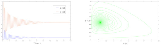
Figure 4. The time histories and the solution for $m=0.18>m_0$. In this case, the equilibrium is locally asymptotically stable and nearby solutions converge to it.

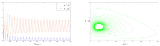
Figure 5. The time histories and the solution for $m=0.14<m_0$. In this case, the equilibrium is no more locally asymptotically stable and a stable limit cycle attracts nearby solutions.

We conclude this section by considering a case in which there are no periodic orbits in $\{y=0\}\cap {\mathbb{R}}_{+}^3$:

Theorem 3.

If

$$r\left(1-\frac{a}{k}\right)+\frac{bk-m(k+a)}{k}<0,$$

(18)

then system (4) does not admit periodic orbits in the set $\{(x,z)\in {\mathbb{R}}^2:x,z\ge 0\}$ .

Proof. 

Let

$$f(x,z)=rx\left(1-\frac{x}{k}\right)-\frac{cxz}{a+x}\mathrm{and}g(x,z)=\frac{bxz}{a+x}-mz.$$

In order to prove the nonexistence of periodic orbits, we use the Bendixson–Dulac theorem that states that if there exists a function $\phi (x,z)$ such that the term

$$\Delta (x,z)=\frac{\partial \left(\phi f\right)}{\partial x}+\frac{\partial \left(\phi g\right)}{\partial z}$$

does not change sign in a simply connected set $\mathcal{S}$, then there are no periodic orbits on $\mathcal{S}$.

We consider then function $\phi (y,z)=(a+x)/x$; then:

$$\Delta (x,z)=r-\frac{a}{k}r+b-m-2\frac{r}{k}x-\frac{am}{x}.$$

We observe that, since $\dot{x}<0$ for $x\ge k$, there are no periodic orbits in the set

$$\{(x,z)\in {\mathbb{R}}_{+}^2:x\ge k\},$$

and for the same reason, there are no periodic orbits crossing the half line $\{x=k,z\ge 0\}$. As a consequence we will restrict to the case $x\le k$ for which we obtain

$$\Delta (x,z)<r-{\displaystyle \frac{a}{k}}r+b-m-{\displaystyle \frac{am}{k}}.$$

Then, $\Delta (x,z)<0$ in $\{(x,z)\in {\mathbb{R}}_{+}^2:x\le k\}$ if $r-\frac{a}{k}r+b-m-\frac{am}{k}$$<0$, and we conclude that there are no periodic orbits in the whole set $\{(x,z)\in {\mathbb{R}}_{+}^2\}$. □

Remark 1.

We observe that, for $a<k$, the condition of Theorem 3 on the nonexistence of periodic orbits

$$r\left(1-\frac{a}{k}\right)+b<m\frac{a+k}{k},$$

that is

$$m>r\frac{k-a}{k+a}+\frac{bk}{k+a},$$

implies

$$m>b\frac{k-a}{k+a},$$

and then is compatible with the results of bifurcation analysis.

3. Existence and Stability Analysis of Equilibria

The first step for studying the dynamics of the system (2) is to find all the equilibrium points and analyzing their stability.

Theorem 4.

System (2) has the following boundary equilibria on $\partial {\mathbb{R}}_{+}^3$:

• $E_0=(0,0,0)$ for any values of the parameters,
• $E_1=(k,0,0)$ for any values of the parameters,
• If $kb>m(a+k)$, the equilibrium $E_2=(ma/(b-m),0,\overline{z})$ with

  $$\overline{z}=\frac{r}{c}\left(\frac{ba}{b-m}\right)\left(1-\frac{ma}{k(b-m)}\right).$$

Proof. 

From direct calculation. □

We also analyze the existence of nontrivial positive equilibria for system (2).

Theorem 5.

The system (2) has at least one positive equilibrium $E^{*}(x^{*},y^{*},z^{*})$ if and only if

$$\beta cm-b(\delta +L)r{x}^{*}\left(1-\frac{x^{*}}{k}\right)>0.$$

(19)

where $x^{*}$ is a solution of the equation

$$C_4{x}^4+C_3{x}^3+C_2{x}^2+C_{1}x+C_0=0.$$

(20)

with the coefficients $C_i,i=0,...,4$ defined below.

Proof. 

By direct calculation, we obtain the equilibrium $E^{*}=(x^{*},y^{*},z^{*})$, with

$$\begin{array}{cc}\hfill & z^{*}=\frac{\beta }{\delta +L},\hfill \\ \hfill & y^{*}=\frac{mc}{\gamma c+bL}-\frac{(\delta +L)b}{\beta (\gamma c+bL)}r{x}^{*}\left(1-\frac{x^{*}}{k}\right),\hfill \end{array}$$

and $x^{*}$ is the solution of the equation

$$C_4{x}^4+C_3{x}^3+C_2{x}^2+C_{1}x+C_0=0.$$

(21)

We must require that $x^{*}$ verifies

$$\beta cm-b(\delta +L)r{x}^{*}\left(1-\frac{x^{*}}{k}\right)>0$$

so that $y^{*}$ is positive. This is always verified if

$$kbr\frac{\delta +L}{\beta }<4cm.$$

(22)

Otherwise, this is satisfied when

$$x^{*}\in \left(0,\frac{k}{2}-\sqrt{\frac{k^2}{4}-\frac{k\beta cm}{br(\delta +L)}}\right)\cup \left(\frac{k}{2}+\sqrt{\frac{k^2}{4}-\frac{k\beta cm}{br(\delta +L)}},\infty \right).$$

(23)

The expressions of the coefficients in Equation (21) are given by

$$\begin{array}{cc}\hfill C_4=& \frac{\gamma }{{(\gamma c+bL)}^2}\frac{{(\delta +L)}^2}{{\beta }^2}\frac{b^2{r}^2}{k^2}\omega ,\hfill \\ \hfill C_3=& \frac{\gamma }{{(bL+c\gamma )}^2}\frac{\delta +L}{\beta }\frac{br}{k}\left(-2\frac{\delta +L}{\beta }\omega br+\gamma c+bL\right),\hfill \\ \hfill C_2=& \frac{\gamma }{{(bL+c\gamma )}^2}\frac{\delta +L}{\beta }\frac{br}{k}\left(m\omega \frac{c\gamma -bL}{\gamma }+(a-k)(\gamma c+bL)+\frac{\delta +L}{\beta }\omega brk\right),\hfill \\ \hfill C_1=& \frac{1}{{(\gamma c+bL)}^2}\left(br\frac{\delta +L}{\beta }\left((m\omega -\gamma a)(\gamma c+bL)-2m\omega \gamma c\right)+\gamma cm(\gamma c+bL)+\right.\hfill \\ \hfill & \left.(b-m){(\gamma c+bL)}^2\right),\hfill \\ \hfill C_0=& \left(ma+\frac{\omega m^{2}c}{\gamma c+bL}\right)\left(\frac{\gamma c}{bL+c\gamma }-1\right).\hfill \end{array}$$

We apply Descartes rule of signs in Equation (21) to study the existence of positive roots. The coefficient of degree zero, $C_0$, is always negative and the coefficient of degree four, $C_4$, is always positive. This means that there always exist a real positive and a real negative zero of the polynomial. The other two zeroes can be complex or real with the same sign.

The other coefficients of the polynomial can be positive, negative or zero, and combining all the possible signs we obtain that:

• If one of the following conditions holds
  • $C_1>0$ and $C_3<0$.
  • $C_1>0$, $C_2<0$ and $C_3=0$.
  • $C_1=0$, $C_2>0$ and $C_3<0$.
  • The signs of $C_3$, $C_1$ and $-C_2$ are equal.
  then there exists three or one positive roots of Equation (21).
• In any other case, there exists one positive root of Equation (21).

So that there exist at least one non-trivial interior equilibrium $E^{*}=(x^{*},y^{*},z^{*})$ of the system (2) if condition (19) is satisfied. □

Corollary 1.

A sufficient condition for the system (2) has at least one positive equilibrium $E^{*}(x^{*},y^{*},z^{*})$ is $kbr\frac{\delta +L}{\beta }<4cm$.

Remark 2.

The positive equilibria, if they exist, are all on the plane $z=\beta /(\delta +L)$.

Remark 3.

Numerically, we have found different cases acording to the existence of positive solutions for the Equation (21) and the existence of positive equilibria $E^{*}$.

• There exist systems for which there is only one positive solution $x^{*}$ of Equation (21), and this solution is such that verifies condition (19). As an example the system with parameters:

  $$a=1/4,b=m=1/2,c=\omega =r=\beta =\delta =L=k=\gamma =1.$$
• There are systems for which there is only one positive solution $x^{*}$ of Equation (21), and this solution does not verify condition (19), so there are no positive equilibria for system (2). As an example the system with parameters:

  $$a=b=c=r=\beta =\delta =k=\gamma =1,\omega =4,L=1/4,m=0.2.$$
• There are systems for which there are three positive solutions $x^{*}$ of Equation (21), and only for one of this solutions condition (19) holds, so there are one positive equilibrium for system (2). As an example the system with parameters:

  $$a=\beta =1/10,b=r=\delta =L=1/2,c=1,\omega =2,k=\gamma =2,m=0.2.$$
• Also there are systems for which there are three positive solutions $x^{*}$ of Equation (21), and none of them verifies condition (19), so system (2) has none positive equilibria. As an example the system with parameters:

  $$a=\beta =1/4,b=\delta =L=1/2,c=1,\omega =k=\gamma =2,r=1m=0.2.$$

We have not found, numerically, any conditions for which Equation (21) has three positive solutions $x^{*}$ and the three of them verify condition (19) but we are not able to exclude this case analytically.

We will analyze the local stability of the equilibria. To do this we consider the Jacobian functional of the vector field

$$J(x,y,z)=\left(\begin{array}{ccc}{f_1}_x& {f_1}_y& {f_1}_z\\ 0& \beta -(\delta +L)z& -y(\delta +L)\\ {f_3}_x& {f_3}_y& {f_3}_z\end{array}\right)$$

where

$$\begin{array}{cc}\hfill & {f_1}_x=r-\frac{2r}{k}x-\frac{(a+\omega y)cz}{{(a+\omega y+x)}^2},{f_1}_y=\frac{\omega cxz}{{(a+\omega y+x)}^2}+Lz,{f_1}_z=-\frac{cx}{a+\omega y+x}+Ly,\hfill \\ \\ \hfill & {f_3}_x=\frac{(a+\omega y)bz}{{(a+\omega y+x)}^2},{f_3}_y=-\frac{\omega bxz}{{(a+\omega y+x)}^2}+\gamma z,{f_3}_z=\frac{bx}{a+\omega y+x}+\gamma y-m,\hfill \end{array}$$

and where we have set for simplicity $\omega =\alpha \eta$.

Theorem 6.

The stability of the boundary equilibria is the following:

• The equilibrium point $E_0$ is always a saddle, the z-axis is the stable manifold and it has an unstable manifold of dimension two.
• The equilibrium point $E_1$ is a saddle with a stable manifold of dimension one if $bk>m(a+k)$ and with a stable manifold of dimension two if $bk<m(a+k)$.
• The equilibrium point $E_2$ is unstable if $\beta >\overline{z}(L+\delta )$ or if $\beta <\overline{z}(L+\delta )$ and one of the following statements holds:
  • $A_2<0$ and condition (7) holds,
  • $A_2>0$ and $A_1>0$.
  The equilibrium point $E_2$ is asymptotically stable if $\beta <\overline{z}(L+\delta )$ and one of the following statements holds:
  • $A_2<0$ and condition (8) holds,
  • $A_2>0$ and $A_1<0$.
  where the coefficients $A_i$ are the ones given in (6).

Proof. 

The local stability analysis of the equilibria $E_0$ and $E_1$ is the same as in the case without indirect effects.

For the equilibrium $E_0=(0,0,0)$ the Jacobian matrix is

$$J\left(E_0\right)=\left(\begin{array}{ccc}r& 0& 0\\ 0& \beta & 0\\ 0& 0& -m\end{array}\right)$$

so there are two positive eigenvalues and one negative eigenvalue so that $E_0$ is a saddle with a stable manifold of dimension one, which is the z-axis, and an unstable manifold of dimension two.

For the equilibrium $E_1=(k,0,0)$ we have

$$J\left(E_1\right)=\left(\begin{array}{ccc}-r& 0& -{\displaystyle \frac{ck}{a+k}}\\ 0& \beta & 0\\ 0& 0& {\displaystyle \frac{bk}{a+k}}-m\end{array}\right).$$

Then, if

$$bk\ne m(a+k),$$

$E_1$ is a saddle, with two positive eigenvalues and one negative eigenvalue if

$$bk>m(a+k),$$

and with one positive eigenvalue and two negative eigenvalues if

$$bk<m(a+k).$$

When the value of $bk$ surpasses the value of $m(a+k)$, a new equilibrium $E_2=(ma/(b-m),0,\overline{z})$ appears, and the equilibrium $E_1$ changes from having an unstable manifold of dimension two to an unstable manifold of dimension one. The functional Jacobian of $E_2$ is

$$J\left(E_2\right)=\left(\begin{array}{ccc}-{\displaystyle \frac{mr\left(k\right(m-b)+a(m+b\left)\right))}{bk(b-m)}}& {\displaystyle \frac{r(bk-m(a+k))(a{b}^{2}L+cm\omega (b-m))}{bck{(b-m)}^2}}& -{\displaystyle \frac{cm}{b}}\\ 0& \beta +{\displaystyle \frac{abr(L+\delta )\left(m\right(a+k)-bk)}{ck{(b-m)}^2}}& 0\\ {\displaystyle \frac{r(bk-m(a+k\left)\right)}{ck}}& {\displaystyle \frac{r(bk-m(a+k\left)\right(ab\gamma +m\omega (m-b)\left)\right)}{ck{(b-m)}^2}}& 0\end{array}\right)$$

(24)

with eigenvalues

$${\lambda }_1=\beta +{\displaystyle \frac{ab\left(m\right(a+k)-bk)r(L+\delta )}{ck{(b-m)}^2}},{\lambda }_{2,3}={\displaystyle \frac{A_1\pm \sqrt{A_2}}{A_3}},$$

(25)

with the coefficients $A_i$ given in (6).

The sign of eigenvalues ${\lambda }_{2,3}$ has been analyzed in Section 2. We note that the expression

$$\frac{-abr(L+\delta )\left(m\right(a+k)-bk)}{ck{(b-m)}^2}$$

can be written as $\overline{z}(L+\delta )$, so we conclude that the eigenvalue ${\lambda }_1$ is positive if

$$\overline{z}<\frac{\beta }{L+\delta },$$

(26)

and it is negative in the other case. Combining the different possibilities for the three eigenvalues we obtain the conditions for the stability of $E_2$. □

Remark 4.

We recall that in the case $\beta =\overline{z}(L+\delta )$, the equilibrium point $E_2$ has two non-zero eigenvalues in the plane $y=0$, as stated in Section 2, and the third eigenvalue is zero. The direction on the flow in the y-direction is determined by the z coordinate. Note that in this case $\dot{y}=y(L+\delta )(\overline{z}-z)$, so $\dot{y}$ is positive if $z<\overline{z}$ and $\dot{y}$ is negative if $z>\overline{z}$.

Remark 5.

We have seen that if (22) is verified then there exists at least one positive equilibrium $E^{*}$. We can prove that, at least in this case, the first eigenvalue ${\lambda }_1$ of $J\left(E_2\right)$ is positive, that is $E_2$ is unstable. We recall that ${\lambda }_1$ is positive if

$$\overline{z}=\frac{r}{c}\left(\frac{ba}{b-m}\right)\left(1-\frac{ma}{k(b-m)}\right)\le \frac{\beta }{L+\delta }.$$

In this case we observe that $\overline{z}\le {\displaystyle \frac{kbr}{4cm}}$, in fact

$$\frac{r}{c}\left(\frac{ba}{b-m}\right)\left(1-\frac{ma}{k(b-m)}\right)\le \frac{kbr}{4cm},$$

can be rewritten as

$${[k(b-m)-2ma]}^2\ge 0,$$

which is always verified.

When all boundary equilibrium points are unstable we expect that there exist solutions that are attracted by an interior equilibrium or a limit cycle.

Theorem 7.

The positive equilibrium $E^{*}$ is locally asymptotically stable if and only if $s_1,s_2,s_3>0$ and $s_1{s}_2-s_3>0$, where the constants $s_1,s_2,s_3$ are defined below.

Proof. 

The characteristic polynomial of $J\left(E^{*}\right)$ is given by the following expression:

$${\lambda }^3+s_1{\lambda }^2+s_2\lambda +s_3=0$$

(27)

where

$$s_1=-Tr\left(J\left(E^{*}\right)\right),s_2=\left|\begin{array}{cc}{f_1}_x& {f_1}_y\\ 0& 0\end{array}\right|+\left|\begin{array}{cc}{f_1}_x& {f_1}_z\\ {f_3}_x& 0\end{array}\right|+\left|\begin{array}{cc}0& -y^{*}(\delta +L)\\ {f_3}_y& 0\end{array}\right|,s_3=-det\left(J\left(E^{*}\right)\right),$$

it is,

$$\begin{array}{cc}\hfill s_1=& m+r\left(\frac{2x^{*}}{k}-1\right)-\gamma y^{*}+\frac{c\beta x^{*}-(c\beta +b{x}^{*}(L+\delta ))(a+x^{*}+y^{*}\omega )}{(L+\delta ){(a+x^{*}+\omega y^{*})}^2},\hfill \\ \hfill s_2=& m\left(r-\frac{2r{x}^{*}}{k}+\frac{c\beta (a+\omega y^{*})}{(L+\delta ){(a+x^{*}+\omega y^{*})}^2}\right)-\frac{1}{k(L+\delta ){(a+x^{*}+\omega y^{*})}^3}\hfill \\ \hfill & \left(\gamma y^{*}(L+\delta )(k(r+\beta )-2r{x}^{*}){(a+x^{*}+\omega y^{*})}^3+(bL(r(k-2x^{*})x^{*}-k\beta (x^{*}+y^{*}))\right.\hfill \\ \hfill & +ck\beta \gamma y^{*}+b\delta x^{*}(kr-2r{x}^{*}-k\beta )){(a+x^{*}+\omega y^{*})}^2+k\beta x^{*}\left(b\right(2c+L(a+x^{*}+y^{*})\hfill \\ \hfill & \left.+\delta (a+x^{*})-c\gamma y^{*}\left)\right)(a+x^{*}+\omega y^{*})-2bck\beta {\left(x^{*}\right)}^2\right),\hfill \end{array}$$

(28)

$$\begin{array}{cc}\hfill s_3=& \frac{\beta }{k(L+\delta ){(a+x^{*}+\omega y^{*})}^4}\left(r\gamma y^{*}(k-2x^{*})(L+\delta ){(a+x^{*}+\omega y^{*})}^4+(bk(Lr{x}^{*}+L\beta y^{*}+r\delta x^{*})\right.\hfill \\ \hfill & -ck\beta \gamma y^{*}-2br{\left(x^{*}\right)}^2(L+\delta )){(a+x^{*}+\omega y^{*})}^3+x^{*}\left(abr(k-2x^{*})(L+\delta )-ck\beta \gamma y^{*}\right.\hfill \\ \hfill & \left.-2br\left(x^{*}\right)(L+\delta )+bk(Lr{x}^{*}-2c\beta +L\beta y^{*}+r\delta x^{*})\right){(a+x^{*}+\omega y^{*})}^2\hfill \\ \hfill & \left.+2bck\beta x^{*}(a+2x^{*})(a+x^{*}+\omega y^{*})-2bck\beta {\left(x^{*}\right)}^2(a+x^{*})\right).\hfill \end{array}$$

We use Hurwitz criterion to study the stability of the equilibrium point $E^{*}$, and we conclude that it is asymptotically stable if and only if $s_1,s_2,s_3>0$ and also the expression $s_1{s}_2-s_3$ is positive. □

Remark 6.

We observe that if $x^{*}\in \left(\frac{k}{2}+\sqrt{\frac{k^2}{4}-\frac{k\beta cm}{br(\delta +L)}},\infty \right)$ then ${f_1}_x$ is negative, that is $Trace\left(J\left(E^{*}\right)\right)<0$. This means that at least one eigenvalue has negative real part.

4. Some Remarks about Coexistence of the Three Species

The problem of the coexistence of the three species can be reformulated in mathematical terms by finding the conditions for which the positive solutions starting in the interior of ${\mathbb{R}}_{+}^3$ do not approach the boundary of the set, $\partial {\mathbb{R}}_{+}^3$ as $t\to +\infty$. These ideas can be made rigorous in the context of persistence theory (see [16]). There are several definitions that are used by mathematicians depending on the context. If we consider a nonlinear system of the form

$$\dot{x}\left(t\right)=f\left(x\right),x\in {\mathbb{R}}_{+}^n$$

(29)

then we have persistence (see [30]) if

$$x_i\left(0\right)>0,i=1,\dots ,n\Rightarrow \underset{t\to +\infty }{lim\; sup}{x}_i\left(t\right)>0,i=1,\dots ,n$$

while we have permanence (see [31]) if there exists $m,M>0$, independent of $x_i\left(0\right)>0$, such that

$$m\le \underset{t\to +\infty }{lim\; inf}x\left(t\right)\le \underset{t\to \infty }{lim\; sup}x\left(t\right)\le M.$$

Finally, we have uniform persistence (see [32]) if there exists $\epsilon >0$, independent of $x_{\left(0\right)}>0$, such that

$$\underset{t\to +\infty }{lim\; inf}x\left(t\right)\ge \epsilon .$$

In many cases, the favorite choice for analysis is uniform persistence, since in real cases, requiring that ${lim\; sup}_{t\to +\infty }{x}_i\left(t\right)>0$ is not sufficient. In fact, a small stochastic or non-autonomous perturbations may lead solutions converges to the boundary. For this reason, in general, it is important to require that ${lim\; sup}_{t\to +\infty }{x}_i\left(t\right)\ge \epsilon >0$. We recall the definition introduced in [17]:

Definition 1.

The system (29) is uniformly $\rho -$persistent if there exists $\epsilon >0$ such that

$$\underset{t\to +\infty }{lim\; inf}\rho \left(x\left(t\right)\right)>\epsilon ,$$

for $x\left(0\right)$ such that

$$\rho \left(x\left(0\right)\right)>0,x\left(0\right)\in {\mathring{\mathbb{R}}}_{+}^3,$$

and where

$$\rho \left(x\right)=min\{x_1,x_2,\dots ,x_n\}.$$

In order to prove uniform persistence (see Theorem 8.17 page 188, hypothesis (H) page 185 and Theorem 5.2 page 126 in [16]), we would need to prove the following conditions:

Hypothesis 1

(H1). There exists a compact attractor of bounded set.

Hypothesis 2

(H2). The invariant sets of $\partial {\mathbb{R}}_{+}^3$ are weakly $\rho -$repelling.

Hypothesis 3

(H3). The invariant sets of $\partial {\mathbb{R}}_{+}^3$ are acyclic.

Unfortunately, in the case of system (29), we cannot prove the existence of a compact attractor of bounded set of ${\mathbb{R}}_{+}^3$ and as a consequence we are not able to obtain uniform persistence of the system. This lack of dissipativity can be guessed by considering the unbounded solutions on the invariant plane $z=0$. Moreover, we recall that the divergence of the vector field F associated to the system

$$divF={f_1}_x+\beta -(\delta +L)z+{f_3}_z,$$

is related to the evolution of the three dimensional volumes elements under the flow of the system. We observe that it has a complex expression, in particular, there are no values of the parameters for which it has a negative sign (which means contraction), on a region of $\partial {\mathbb{R}}_{+}^3$. Moreover, while the first term and the second term are negative for high values of x and z respectively, the third term is positive for high value of y.

Then, we are able only to prove conditions (H2)–(H3) which only ensures that the invariant sets of $\partial {\mathbb{R}}_{+}^3$ does not attracts positive solutions. For condition (H2) we first recall the definition:

Definition 2.

A set $M\subset {\mathbb{R}}_{+}^3$ is called is called weakly $\rho -$repelling if there is no solution $x\left(t\right)$ of system (29) starting at $x_0$, with $\rho \left(x_0\right)>0$, such that $x\left(t\right)\to M$ as $t\to +\infty$.

Theorem 8.

We suppose that hypothesis of Theorem 3 is verified. Then the invariant set of $\partial {\mathbb{R}}_{+}^3$ are weakly $\rho -$repelling in any of the following cases

(1)

$bk<k(a+m)$;

(2)

$bk>k(a+m)$ and $\beta >{\displaystyle \frac{ab(bk-m(a+k\left)\right)r(L+\delta )}{ck{(b-m)}^2}}$.

Proof. 

In order to prove the theorem, it is sufficient to show that the stable manifolds of the invariant sets of $\partial {\mathbb{R}}_{+}^3$ are contained all contained in $\partial {\mathbb{R}}_{+}^3$.

The equilibria $E_0$ and $E_1$ have their stable manifolds on $\partial {\mathbb{R}}_{+}^3$ for any value of the parameters. Then if

$$b-k(m+a)<0,$$

there are no further equilibria. Otherwise, if $E_2$ exists, a sufficient condition that ensures that its stable manifold is in $\partial {\mathbb{R}}_{+}^3$ consists in requiring that

$$\beta >{\displaystyle \frac{ab(bk-m(a+k\left)\right)r(L+\delta )}{ck{(b-m)}^2}},$$

(30)

that is, its first eigenvalues is positive. To conclude the proof we have to exclude the existence of other invariant set contained in $\partial {\mathbb{R}}_{+}^3$. We use Theorem 3 that guarantees the non existence of periodic orbits in the plane $y=0$, that is the only invariant sets of $\partial {\mathbb{R}}_{+}^3$ are the equilibria. □

Now we pass to check condition (H3).

Definition 3.

Let $A,B\subset \partial {\mathbb{R}}_{+}^3$. Then A is chained to B in $\partial {\mathbb{R}}_{+}^3$, and we write $A\Rightarrow$ if there exists a total trajectory $x\left(t\right)$ with $x\left(0\right)\notin A\cup B$ such that

$$x(-t)\to A,x\left(t\right)\to B,\mathrm{for}t\to +\infty .$$

Definition 4.

A finite collection $\{M_1,\dots ,M_k\}$ of subsets of $\partial {\mathbb{R}}_{+}^3$ is called cyclic if after possibly renumbering $M_1\Rightarrow M_1$ or $M_1\Rightarrow M_2\Rightarrow \dots \Rightarrow M_j\Rightarrow M_1$ in $\partial {\mathbb{R}}_{+}^3$ for some $j\in \{2,\dots ,k\}$. Otherwise it is called acyclic.

Thanks to this notion we are able to exclude the case in which orbits are attracted by an heteroclinic cycle that connects the equilibria such as in the well known case of [33].

Theorem 9.

If hypothesis of Theorem 3 is verified, then the invariant sets $\{E_0,E_1,E_2\}$ of $\partial {\mathbb{R}}_{+}^3$ are acyclic.

Proof. 

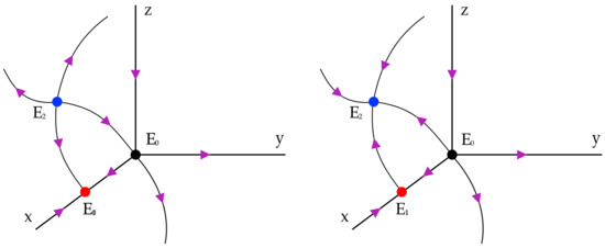
By hypothesis the only invariant sets of $\partial {\mathbb{R}}_{+}^3$ are equilibria. The analysis of the previous sections is sufficient to exclude the existence of cycle between equilibria. In Figure 6 below we represent the case in which there are only two boundary equilibria ($E_0$ and $E_1$) while in Figure 7 we represent the case in which we have also $E_2$. In the latter situation we distinguish two cases: both eigenvalues with positive and both with negative real part respectively. □

Figure 6. Possible connections in the cases in which there exist only two boundary equilibria.

Figure 7. Possible connections in the cases in which there exists three boundary equilibria. In the first case the eigenvalues ${\lambda }_{2,3}$ of $J\left(E_2\right)$ both have positive real part while in the second they have negative real part.

In conclusion, we are not able to prove uniform persistence, however the above results guarantee a sort of weak persistence of the three species.

5. Hopf Bifurcation

In this section, we analyze the possible existence of a limit cycle by Hopf bifurcation for the positive equilibrium $E^{*}$. We recall that Hopf bifurcation occurs when a pair of complex conjugate eigenvalues of the Jacobian matrix of an equilibrium crosses the imaginary axis. In this case a limit cycle arises and its stability character can be obtained by the analysis of the first Lyapunov coefficient. If it is negative the cycle is stable and the bifurcation is called supercritical; otherwise, it is unstable and the bifurcation is called subcritical.

Because of the complexity of the system and the high number of parameters we are not able to perform a general bifurcation analysis. In this section, we simplify this task by fixing the value of parameters and using m as bifurcation parameter.

In details, we set:

$$\begin{array}{cc}\hfill & a=b=c=\alpha =\eta =r=1,\hfill \\ \hfill & k=\beta =\frac{1}{2},\delta =\frac{4}{10},\gamma =L=\frac{1}{10}.\hfill \end{array}$$

With the above choice of the parameters we have

$$\beta =\delta +L,$$

and as a consequence $z^{*}=1$. In this case the equilibrium is:

$$E^{*}=(x^{*},y^{*},1)$$

where

$$y^{*}=5\left[m-x^{*}+2{\left(x^{*}\right)}^2\right]$$

and $x^{*}$ is the solution of the equation

$$D_4{x}^4+D_3{x}^3+D_2{x}^2+D_{1}x+D_0=0,$$

with

$$\begin{array}{cc}\hfill & D_4=10>0,D_3=-9<0,D_2=3>0,\hfill \\ \hfill & D_1=-\frac{1}{2}(m-1),D_0=-\frac{1}{2}m(1+5m).\hfill \end{array}$$

Moreover the functional Jacobian at $E^{*}$ is

$$J\left(E^{*}\right)=\left(\begin{array}{ccc}{f_1}_x& {f_1}_y& {f_1}_z\\ 0& 0& -\frac{1}{2}{y}^{*}\\ {f_3}_x& {f_3}_y& 0\end{array}\right)$$

where

$$\begin{array}{cc}\hfill & {f_1}_x=1-4x^{*}-\frac{(1+y^{*})}{{(1+x^{*}+y^{*})}^2},{f_1}_y=\frac{x^{*}}{{(1+x^{*}+y^{*})}^2}+\frac{1}{10},{f_1}_z=-\frac{x^{*}}{1+x^{*}+y^{*}}+\frac{1}{10}{y}^{*},\hfill \\ \hfill & {f_3}_x=\frac{(1+y^{*})}{{(1+x^{*}+y^{*})}^2},{f_3}_y=-\frac{x^{*}}{{(1+x^{*}+y^{*})}^2}+\frac{1}{10}.\hfill \end{array}$$

The characteristic polynomial is

$$p\left(\lambda \right)={\lambda }^3+s1{\lambda }^2+s_2\lambda +s_1$$

where

$$s_1=-{f_1}_x=-Tr\left(J\left(E^{*}\right)\right),s_2=-{f_1}_z{f_3}_x+y^{*}(\delta +L){f_3}_y,s_3-y^{*}(\delta +L)\left[{f_1}_x{f_3}_y-{f_1}_y{f_3}_x\right].$$

The Hurwitz matrix of the characteristic polynomial is given by

$$H\left(p\right)=\left(\begin{array}{ccc}1& s_2& 0\\ s_1& s_3& 0\\ {\displaystyle \frac{s_1{s}_2-s_3}{s_1}}& 0& 0\end{array}\right).$$

If $s_1>0$, we always have a negative (real) eigenvalue, while if $p^{\prime }\left(\lambda \right)>0$, that is $s_1^2-3s_2<0$, we ensure that the other two eigenvalues are complex conjugate. If $s_1{s}_2-s_3>0$ (resp. $<0$) then we have at least two eigenvalues with negative (resp. positive) real part.

From Hurwitz-Routh criterion we obtain that a necessary condition for Hopf Bifurcation in this case becomes

$$s_1{s}_2-s_3={f_3}_x\left[{f_1}_x{f_1}_z-\frac{1}{2}{y}^{*}{f_1}_y\right]=0,$$

that is

$${f_1}_x{f_1}_z-\frac{1}{2}{y}^{*}{f_1}_y=0.$$

We have numerically solved the previous equation by using the software Matlab and we obtained the critical value

$$m_H=0.2617.$$

For this value we obtain $s_1=0.215694$, $s_2=-0.0410984$, $s_3=-0.0306826$ and $s_1^2-3s_2=0.169819$.

For $m=m_H$ the eigenvalues of the Jacobian matrix $J\left(E^{*}\right)$ are

$${\lambda }_1=-0.9395,{\lambda }_{2,3}=\pm 0.2027i.$$

We will see below that as m passes trough the value $m=m_H$ the real part of the eigenvalues ${\lambda }_{2,3}$ change sign from negative to positive.

Then a cycle appears due to Hopf Bifurcation of the equilibrium $E^{*}$. We are not able to exactly compute the first Lyapunov exponent of the system, however simulations and the sign of the term $s_1{s}_2-s_3$ suggests that the cycle is stable and the equilibrium looses stability. In Figure 8 below we represents the solutions for $m=m_H$, as we expect, they converge to a periodic solution of period $T=\frac{2\pi }{0.2027}=30.9975$.

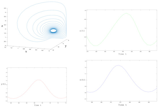
Figure 8. A limit cycle arises for $m=m_H$. We have represented the solution and a zoom showing the period ($T=30.9975$) of its three components.

In order to illustrate the results of this section we present several numerical simulations. We fix the parameters as above and initial data as follows.

$$x\left(0\right)=y\left(0\right)=z\left(0\right)=\frac{1}{10}.$$

In a first numerical experiment we fix $m=2/10<m_H$ and as we expect solutions converges to the equilibrium (see Figure 9 below)

$$E^{*}=(0.2668,0.3778,1).$$

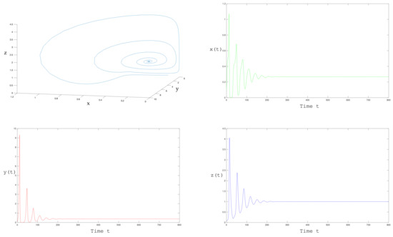
Figure 9. Graphic and time series of the solution for $m=2/10<m_H$. The positive equilibrium $E^{*}$ is locally stable and nearby solutions converge to it.

In this case the eigenvalues of $J\left(E^{*}\right)$ are

$${\lambda }_1=-0.5252,{\lambda }_{2,3}=-0.0257\pm 0.1898i,$$

and have negative real parts.

In a second numerical experiment, we set $m=4/10>m_H$. The positive equilibrium point

$$E^{*}=(0.595,2.57,1)$$

is unstable, the eigenvalues of $J\left(E^{*}\right)$ are

$${\lambda }_1=-1.6157,{\lambda }_{2,3}=0.0136\pm 0.3237i.$$

We observe that the eigenvalues ${\lambda }_{2,3}$ now have positive real part and a Hopf bifurcation occurs at $m_H=0.2617$. Solutions converge to a limit cycle as shown in Figure 10.

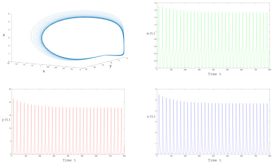
Figure 10. Graphic and time series of the solution for $m=4/10>m_H$. The positive equilibrium $E^{*}$ is unstable and solutions converge to a stable limit cycle.

6. Conclusions

In this paper, we have considered a model describing the dynamics of an ecological system with two prey species and a predator species, which is a modification of the model proposed in [1]. In particular, due to the high availability of one of the two prey populations, we supposed that the predator prefer to predate the more available prey population whereas the other one take advantages of it. In previous articles in the literature (see Introduction for details), it has been pointed out the importance of indirect effects in order to describe real cases of coexistence.

We have performed the stability analysis of equilibria and we have made a detailed analysis of the system on the invariant planes, including the study of the existence of Hopf bifurcation at the equilibrium point $E_2$. We have proved that through this bifurcation a stable limit cycle appears.

Regarding the existence of positive equilibria, the expression (21) and the verification of one of the conditions (22) or (23) give us all the positive equilibrium points. The expressions of the equilibria as a function of the parameters are too complicated and not easy to handle. Because of this, we have not been able to determine, in general, for which conditions appear none, one or three equilibria. We have obtained sufficient conditions for the existence of at least one positive equilibrium (see Corollary 1). Also, for fixed values of the parameters it is easy to compute the positive equilibria and maybe it would be possible for certain subfamilies on which less parameters are considered.We have found values of the parameters for which there exist one equilibrium point, and others for which there are not any positive equilibria, but numerically, we have not found values for which three positive equilibria exist, and therefore we think that probably this situation is not feasible, although we have not been able to prove it.

We have shown that Hopf bifurcation can occur also at the positive equilibrium $E^{*}$ and as a consequence, coexistence of the three species via the existence of an attracting limit cycle is possible, by taking into account indirect effects of predation. It is worth mentioning that in [1] Hopf bifurcation is obtained only by considering a version of the model with time delay.

Furthermore, we have included a detailed discussion about the problem of persistence of the system.

Throughout the paper, several numerical simulations are provided in order to illustrate the theoretical results.

Due to the complexity of the model, we have not been able to perform a complete bifurcation analysis, then this point remains as an open problem and it would be interesting to study it in the future. A further analysis of predator prey models incorporating indirect effects can be done, for example, considering time delay or non autonomous (seasonal) terms.

A final comment for further research: the proposed model in this paper could be easily implemented by using analog devices ([34]). Therefore, it could be used to perform experiments in this way.

References

- Sharma, S.; Samanta, G.P. Dynamical Behaviour of a Two Prey and One Predator System. Differ. Eq. Dyn. Syst. 2014, 22, 125–145. [Google Scholar] [CrossRef]
- Bolker, B.; Holyoak, M.; Krivan, V.; Rowe, L.; Schmitz, O. Connecting theoretical and empirical studies of trait-mediated interactions. Ecology 2003, 84, 1101–1114. [Google Scholar] [CrossRef]
- Cariveau, D.; Irwin, R.E.; Brody, A.K.; Garcia-Mayeya, L.S.; von der Ohe, A. Direct and indirect effects of pollinators and seed predators to selection on plant and floral traits. Oikos 2004, 104, 15–26. [Google Scholar] [CrossRef]
- Gomez, J.; Zamora, R. Top-down effects in a tritrophoc system: Parasitoids enhance plant fitness. Ecology 1994, 75, 1023–1030. [Google Scholar] [CrossRef]
- Hessen, D.O.; Andersen, T.; Brettum, P.; Faafeng, B.A. Phytoplankton contribution to sestonic mass and elemental ratios in lakes: Implications for zooplankton nutrition. Limnol. Oceanogr. Meth. 2003, 48, 1289–1296. [Google Scholar] [CrossRef]
- Lundgren, V.; Granéli, E. Grazer-induced defense in Phaeocystis globosa (Prymnesiophyceae): Influence of different nutrient conditions. Limnol. Oceanogr. Meth. 2010, 55, 1965–1976. [Google Scholar] [CrossRef]
- Margalef, R. Life forms of Phytoplanktos as survival alternative in an unstable environment. Oceanol. Acta 1978, 134, 493–509. [Google Scholar]
- Menge, B.A. Indirect effects in marine rocky intertidal interaction webs: Patterns and importance. Ecol. Monogr. 1995, 65, 21–74. [Google Scholar] [CrossRef]
- Sarnelle, O. Daphnia as keystone predators: Effects on phytoplankton diversity and grazing resistance. J. Plankton Res. 2005, 27, 1229–1238. [Google Scholar] [CrossRef]
- Snyder, W.E.; Ives, A.R. Generalist predators disrupt biological control by a specialist parasitoid. Ecology 2001, 82, 705–716. [Google Scholar] [CrossRef]
- Walsh, M.R.; Reznick, D.N. Interactions between the direct and indirect effects of predators determine life history evolution in a killifish. Proc. Natl. Acad. Sci. USA 2008, 105, 594–599. [Google Scholar] [CrossRef]
- Wootton, J.T. Indirect effects, prey susceptibility, and habitat selection: Impacts of birds on limpets and algae. Ecology 1992, 73, 981–991. [Google Scholar] [CrossRef]
- Estes, J.; Crooks, K.; Holt, R. Ecological Role of Predators. Enciclopedia Biodivers. 2001, 4, 857–878. [Google Scholar]
- Carusela, M.F.; Momo, F.R.; Romanelli, L. Competition, predation and coexistence in a three trophic system. Ecol. Model. 2009, 220, 2349–2352. [Google Scholar] [CrossRef]
- Colucci, R. Coexistence in a one-predator, two-prey system with indirect effects. J. Appl. Math. 2013, 2013, 625391. [Google Scholar] [CrossRef]
- Smith, H.L.; Thieme, H.R. Dynamical Systems and Population Persistence; American Mathematical Society: Providence, RI, USA, 2011. [Google Scholar]
- Butler, G.; Freedman, H.I.; Waltman, P. Uniformly persistent systems. Proc. Am. Math. Soc. 1968, 96, 425–430. [Google Scholar] [CrossRef]
- Colucci, R.; Nuñez, D. Periodic orbits for a three-dimensional biological differential systems. Abstr. Appl. Anal. 2013, 2013, 465183. [Google Scholar] [CrossRef]
- Caraballo, T.; Colucci, R.; Han, X. Non-autonomous dynamics of a semi-Kolmogorov population model with periodic forcing. Nonlinear Anal. Real World Appl. 2016, 31, 661–680. [Google Scholar] [CrossRef]
- Caraballo, T.; Colucci, R.; Han, X. Semi-Kolmogorov models for predation with indirect effects in random environments. Discret. Contin. Dyn. Syst. 2016, 21, 2129–2143. [Google Scholar] [CrossRef]
- Caraballo, T.; Colucci, R.; Han, X. Predation with indirect effects in fluctuating environments. Nonlinear Dyn. 2016, 84, 115–126. [Google Scholar] [CrossRef]
- Poincaré, H. Mémoire sur les courbes définies par une équation différentielle. J. Math. Pures Appl. 1881, 7, 375–422. [Google Scholar]
- Hilbert, D. Mathematische probleme. Lecture, Second Internat Congr Math. Paris, 1900. Bull. Am. Math. Soc. 1902, 8, 437–479. [Google Scholar] [CrossRef]
- Ilyashenko, Y. Centennial history of Hilbert’s 16th problem. Bull. Am. Math. Soc. 2002, 39, 301–354. [Google Scholar] [CrossRef]
- Li, J. Hilbert’s 16th problem and bifurcations of planar polynomial vector fields. Int. J. Bifurc. Chaos 2003, 13, 47–106. [Google Scholar] [CrossRef]
- Van der Pol, B. The London, Edinburgh and Dublin Philosophical Magazine; Taylor and Francis: London, UK, 1926; pp. 978–992. [Google Scholar]
- Diz-Pita, E.; Llibre, J.; Otero-Espinar, M.V.; Valls, C. The zero-Hopf bifurcations in the Kolmogorov systems of degree 3 in R3. Commun. Nonlinear Sci. Numer. Simul. 2021, 95C. [Google Scholar] [CrossRef]
- Han, M.; Llibre, J.; Tian, Y. On the Zero-Hopf Bifurcation of the Lotka-Volterra Systems in R3. Mathematics 2020, 8, 1137. [Google Scholar] [CrossRef]
- Kuznetsov, Y. Elements of Applied Bifurcation Theory, 2nd ed.; Springer: New York, NY, USA, 1998. [Google Scholar]
- Freedman, H.I.; Waltman, P. Mathematical analysis of some three-species food chain models. Math. Biosci. 1977, 33, 257–276. [Google Scholar] [CrossRef]
- Schuster, P.; Sigmund, K.; Wolff, R. Dynamical systems under constant organization III. Cooperative and competitive behaviour in hypercycles. J. Differ. Eq. 1979, 32, 357–368. [Google Scholar] [CrossRef]
- Hofbauer, J. A general cooperation theorem for hypercycles. Monatshefte Math. 1981, 91, 233–240. [Google Scholar] [CrossRef]
- May, R.M.; Leonard, W.J. Nonlinear Aspects of Competition Between Three Species. SIAM J. Appl. Math. 1975, 29, 243–253. [Google Scholar] [CrossRef]
- Buscarino, A.; Fortuna, L.; Frasca, M. Essentials of Nonlinear Circuit Dynamics with MATLAB® and Laboratory Experiments; CRC Press: Boca Raton, FL, USA, 2017. [Google Scholar] [CrossRef]
Publisher’s Note: MDPI stays neutral with regard to jurisdictional claims in published maps and institutional affiliations. |
© 2021 by the authors. Licensee MDPI, Basel, Switzerland. This article is an open access article distributed under the terms and conditions of the Creative Commons Attribution (CC BY) license (http://creativecommons.org/licenses/by/4.0/).