Multi-Time Generalized Nash Equilibria with Dynamic Flow Applications

Abstract

We propose a multi-time generalized Nash equilibrium problem and prove its equivalence with a multi-time quasi-variational inequality problem. Then, we establish the existence of equilibria. Furthermore, we demonstrate that our multi-time generalized Nash equilibrium problem can be applied to solving traffic network problems, the aim of which is to minimize the traffic cost of each route and to solving a river basin pollution problem. Moreover, we also study the proposed multi-time generalized Nash equilibrium problem as a projected dynamical system and numerically illustrate our theoretical results.

1. Introduction

The concept of an equilibrium problem originated with Cournot [1] in the context of an oligopolistic economy, but formally it was introduced by Nash [2,3]. Therefore, it is called a Nash equilibrium problem. Nash equilibrium problems have been extensively studied and employed as powerful and flexible tools. However, the Nash equilibrium only deals with the dependency of the payoff function of each player on the strategies of the other (rival) players. Later, this notion was extended to the generalized Nash equilibrium by Arrow and Debreu [4], where each player’s strategy set also depends on the strategies of the other players. Generalized Nash equilibrium problems are important in mathematical modeling because of their usefulness in the modeling of economic systems [5], routing problems in communication networks [6], and in engineering applications [7]. The survey papers [8,9] give a complete overview of the state of the art regarding theoretical results and numerical methods for solving generalized Nash equilibrium problems. One of the popular strategies for solving the generalized Nash equilibrium problem is to first bridge the gap between this problem and well-known variational tools in the literature, and then to use these well-developed tools to solve it. Instances of such methods are reformulations of generalized Nash equilibrium problems as suitable variational inequalities and quasi-variational inequalities.

A variational inequality problem comprises an inequality which must be satisfied for all the elements of a given (convex) set. The study of variational inequality problems in traffic analysis was initiated by Smith [10] and Dafermos [11]. They set up the traffic assignment problem in terms of a finite-dimensional variational inequality problem. Presently variational inequalities constitute an important modeling tool in economics [12,13], optimization [14] and game theory [15,16,17]. A quasi-variational inequality problem is an extension of the concept of a variational inequality problem, where the feasible set is also allowed to vary. Such problems have been used to model more complex phenomena. It was Bensoussan [18] who first recognized the connection between the generalized Nash equilibrium and quasi-variational inequality problems, and studied them in Hilbert space. Thereafter, Harker [17] investigated these problems in Euclidean spaces. Aussel et al. [19] studied the time-dependent generalized Nash equilibrium problem and reformulated it as an evolutionary quasi-variational inequality problem. More relevant papers are well documented in [20,21,22].

In recent decades the notion of multi-time has frequently been used in optimization theory and in multi-time control problems. Indeed, several science and engineering problems can be converted into optimization problems that are defined as m-flow type PDEs (multi-time evolution systems) and the associated cost functionals are expressed as path-independent curvilinear integrals or multiple integrals. Udrişte and Ţevy [23] introduced the basic optimization problems involving path-independent curvilinear integrals and multiple integrals. Mathematically speaking, these integrals are equivalent, but their meanings are completely different in real life problems. Thereafter, a systematic study of multi-time problems was initiated by the research group of Udrişte [24,25,26,27]. In this way, a multi-time parameter of evolution approach in optimization theory started to be used and this concept has extensively been explored; see [28,29,30]. Apart from optimization, the concept of a multi-time parameter of evolution is also used in space theory. A space coordinate is merely an index numbering degrees of freedom and the time coordinate is usually the physical time in which the system evolves. In some physical problems, two-time $t=(t_1;t_2)$ is used, where $t_1$ means the intrinsic time and $t_2$ the observer time. These prominent roles of multi-time parameters in different areas of science show the necessity of some new formulations of this concept. To pursue further explorations and present novel results involving multi-time parameters, particularly in optimization and noncooperative games, we formulate the multi-time generalized Nash equilibrium problem (MGNEP), which is a generalized form of the time-dependent generalized Nash equilibrium problem studied by Aussel et al. [19], and reformulate it as a multi-time quasi-variational inequality problem. We also establish the existence of equilibria. To provide an application of the formulated multi-time generalized Nash equilibrium problems in traffic analysis, we interpret a traffic network model in terms of such an equilibrium problem for a courier service company with the intention of minimizing the traffic cost of each route. Moreover, we also provide an application to solving river basin pollution problems. We formulate a river basin pollution problem in terms of our multi-time generalized Nash equilibrium problem, and demonstrate how the industrial factories (agents) situated along a river can maximize their profit by following the particular norms and restrictions of reducing the river water pollution imposed by the basin authorities. Finally, we propose a method for solving the multi-time generalized Nash equilibrium problem via projected dynamical system theory. To exhibit the utility of our proposed method, we solve the well-known Nguyen traffic network problem [31] using this method and numerically illustrate our results.

Our paper is organized as follows: preliminaries and the formulations of the problem are presented in Section 2. The equivalence of the multi-time generalized Nash equilibrium problem with the multi-time quasi-variational inequality problem is established in Section 3. The existence of equilibria is obtained in Section 4. The applications of multi-time generalized Nash equilibrium problems in traffic network analysis and to solving river basin pollution problems are demonstrated in Section 5. Explorations of the multi-time generalized Nash equilibrium problem as a projected dynamical system, as well as numerical illustrations regarding the Nguyen traffic network, are presented in Section 6. Section 7 concludes our paper.

2. Preliminaries and Problem Formulations

We start with the formulation of a multi-time generalized Nash equilibrium problem. To this end, we first introduce important notation and mathematical tools. We consider a hyperparallelepiped ${\mathrm{\Omega }}_{l_{\circ },l_1}$ in ${\mathbb{R}}^m$ with the opposite diagonal points $l_{\circ }=(l_{\circ }^1,l_{\circ }^2,\dots ,l_{\circ }^m)$ and $l_1=(l_1^1,l_1^2,\dots ,l_1^m)$. Using the product order relation on ${\mathbb{R}}^m$, we can view this hyperparallelepiped as an interval ${[l_{\circ },l_1]}^m$. This interval is sometimes called the planning horizon of players for preparing their strategies. We denote by t the multi-time parameter of evolution. It is defined as $t=\left(t^{\alpha }\right)\in {\mathrm{\Omega }}_{l_{\circ },l_1}$, where $\alpha =(1,2,\dots ,m)$. The multi-time generalized Nash equilibrium problem comprises N players and each player $\mu$ controls the variable $x^{\mu }\left(t\right)\in L^2({\mathrm{\Omega }}_{l_{\circ },l_1},{\mathbb{R}}^{n_{\mu }})$. This variable is the multi-time-dependent vector of strategies of the player $\mu$. Let $x^{-\mu }\left(t\right)\in L^2({\mathrm{\Omega }}_{l_{\circ },l_1},{\mathbb{R}}^{n-n_{\mu }})$ be the vector of strategies set up by the decision variables of all the players except the player $\mu$ at a given multi-time $t\in {\mathrm{\Omega }}_{l_{\circ },l_1}$ and let $x\left(t\right)\in L^2({\mathrm{\Omega }}_{l_{\circ },l_1},{\mathbb{R}}^n)$ be the multi-time-dependent vector of strategies of all players. Here $n={\displaystyle {\displaystyle \sum }_{\mu =1}^N}{n}_{\mu }$. When we wish to put the strategy vector of the player $\mu$ under a spotlight, we write the strategy vector $x\left(t\right)$ of all the players as

$$x\left(t\right)=(x^{\mu }\left(t\right),x^{-\mu }\left(t\right)).$$

This is still the vector $x\left(t\right)=(x^1\left(t\right),x^2\left(t\right),\dots ,x^{\mu -1}\left(t\right),x^{\mu }\left(t\right),x^{\mu +1}\left(t\right),\dots ,x^N\left(t\right))$ which belongs to $L^2({\mathrm{\Omega }}_{l_{\circ },l_1},{\mathbb{R}}^n)$. Please note that the notation $(x^{\mu }\left(t\right),x^{-\mu }\left(t\right))$ does not mean that the block components of $x\left(t\right)$ are reordered in such a way so that $x^{\mu }\left(t\right)$ becomes the first block. We hark back to $L^2({\mathrm{\Omega }}_{l_{\circ },l_1},{\mathbb{R}}^n)=L^2({\mathrm{\Omega }}_{l_{\circ },l_1},{\mathbb{R}}^{n_{\mu }})\times L^2({\mathrm{\Omega }}_{l_{\circ },l_1},{\mathbb{R}}^{n-n_{\mu }})$. Now let K be a nonempty, closed and convex subset of $L^2({\mathrm{\Omega }}_{l_{\circ },l_1},{\mathbb{R}}^n)$. For any given strategy vector $x^{-\mu }\left(t\right)$ of the rival players, we denote the nonempty, closed and convex feasible set (or strategy set) of the player $\mu$ by $K_{\mu }\left(x^{-\mu }\left(t\right)\right)$. This is a subset of $L^2({\mathrm{\Omega }}_{l_{\circ },l_1},{\mathbb{R}}^{n_{\mu }})$. Each player has an objective function which is called the cost (or loss, or payoff) function. It depends on the player’s own variables $x^{\mu }\left(t\right)$, as well as on those of the rival players $x^{-\mu }\left(t\right)$. In our formulation of the multi-time generalized Nash equilibrium problem, we write the total cost function $F^{\mu }:L^2({\mathrm{\Omega }}_{l_{\circ },l_1},{\mathbb{R}}^n)\to \mathbb{R}$ of the player $\mu$ as a multiple integral. More precisely,

$$F^{\mu }\left(x\left(t\right)\right)={\int }_{{\mathrm{\Omega }}_{l_{\circ },l_1}}{f}^{\mu }(x^{\mu }\left(s\right),x^{-\mu }\left(s\right))ds,$$

where $f^{\mu }(x^{\mu }\left(s\right),x^{-\mu }\left(s\right))$ is a real-valued continuously differentiable function which denotes the running cost (loss) function the player $\mu$ bears when the rival players have chosen the strategy $x^{-\mu }\left(s\right)$ at a given time $s\in {\mathrm{\Omega }}_{l_{\circ },l_1}$, and $ds=d{s}^1\dots d{s}^m$ denotes the volume element of ${\mathrm{\Omega }}_{l_{\circ },l_1}$. We use the following notation to denote the value of the function represented by $p\left(t\right)$ at the point $q\left(t\right)$:

$$⟨⟨p\left(t\right),q\left(t\right)⟩⟩={\int }_{{\mathrm{\Omega }}_{l_{\circ },l_1}}⟨p\left(s\right),q\left(s\right)⟩ds\forall p\left(t\right),q\left(t\right)\in L^2({\mathrm{\Omega }}_{l_{\circ },l_1},{\mathbb{R}}^n),$$

where $⟨.,.⟩$ represents the Euclidean inner product. Throughout the paper, the abbreviation “a.e.” stands for “almost everywhere" and ${\mathbb{R}}_{+}^p$ represents the set of non-negative vectors in the Euclidean space ${\mathbb{R}}^p$.

Remark 1.

In our paper, we do not impose any special structure on the feasible set $K_{\mu }\left(x^{-\mu }\left(t\right)\right)$ of each player. For studies of generalized Nash equilibrium problems with special structures on the feasible set of each player, we refer the interested readers to [8,21].

Now we are able to introduce our multi-time generalized Nash equilibrium problem (MGNEP). For a given strategy vector $x^{-\mu }\left(t\right)$ of rival players, the aim of a player $\mu$ is to choose a strategy vector $x^{\mu }\left(t\right)$ such that it solves the following multi-time minimization problem:

$$\mathbf{\left(}\mathbf{MGNEP}\mathbf{\right)}\underset{x^{\mu }\left(t\right)}{min}{\int }_{{\mathrm{\Omega }}_{l_{\circ },l_1}}{f}^{\mu }(x^{\mu }\left(t\right),x^{-\mu }\left(t\right))dt,$$

$$\mathrm{subject}\mathrm{to}{x}^{\mu }\left(t\right)\in K_{\mu }\left(x^{-\mu }\left(t\right)\right).$$

Problem (MGNEP) can also be interpreted in the following way.

Definition 1.

A strategy vector $y\left(t\right)\in K$ is said to be a multi-time generalized Nash equilibrium if and only if for each player μ, we have $y^{\mu }\left(t\right)\in K_{\mu }\left(y^{-\mu }\left(t\right)\right)$ and

$${\int }_{{\mathrm{\Omega }}_{l_{\circ },l_1}}{f}^{\mu }(y^{\mu }\left(t\right),y^{-\mu }\left(t\right))dt\le {\int }_{{\mathrm{\Omega }}_{l_{\circ },l_1}}{f}^{\mu }(x^{\mu }\left(t\right),y^{-\mu }\left(t\right))dt\forall x^{\mu }\left(t\right)\in K_{\mu }\left(y^{-\mu }\left(t\right)\right).$$

Special Case. If $m=1$, then ${\mathrm{\Omega }}_{l_{\circ },l_1}$ is simply the closed real interval $[l_{\circ },l_1]$. Furthermore, for more convenience, we put $l_{\circ }=0$ and $l_1=T$ (which denotes an arbitrary time) and then ${\mathrm{\Omega }}_{l_{\circ },l_1}=[0,T]$ (a fixed time interval). Consequently, in this case (MGNEP) reduces to the time-dependent generalized Nash equilibrium problem, studied by Aussel et al. [19].

To formulate our multi-time quasi-variational inequality problem, we define the set-valued map $\mathrm{\Gamma }:K\to 2^K$ by

$$\mathrm{\Gamma }\left(x\left(t\right)\right):={\displaystyle \prod _{\mu =1}^N}{K}_{\mu }\left(x^{-\mu }\left(t\right)\right)$$

for each $x\left(t\right)\in K$. We also let $J:L^2({\mathrm{\Omega }}_{l_{\circ },l_1},{\mathbb{R}}^n)\to L^2({\mathrm{\Omega }}_{l_{\circ },l_1},{\mathbb{R}}^n)$ be a single-valued map. Our multi-time quasi-variational inequality problem is defined as follows:

(MQVIP) to find a vector $y\left(t\right)\in K$ such that $y\left(t\right)\in \mathrm{\Gamma }\left(y\right(t\left)\right)$ and

$${\int }_{{\mathrm{\Omega }}_{l_{\circ },l_1}}⟨J\left(y\left(t\right)\right),x\left(t\right)-y\left(t\right)⟩dt\ge 0\forall x\left(t\right)\in \mathrm{\Gamma }\left(y\left(t\right)\right).$$

Taking into account the definitions of generalized convexities formulated in [32,33], we define the following notion of convexity for a multi-time functional $H:K\to \mathbb{R}$ of the form $H\left(x\left(t\right)\right)={\int }_{{\mathrm{\Omega }}_{l_{\circ },l_1}}h\left(x\left(s\right)\right)ds$, where h is a real-valued continuously differentiable function.

Definition 2.

The multi-time functional H is said to be convex on the set K if for all $x\left(s\right),y\left(s\right)\in K$, the following inequality holds:

$${\int }_{{\mathrm{\Omega }}_{l_{\circ },l_1}}h\left(x\left(s\right)\right)ds-{\int }_{{\mathrm{\Omega }}_{l_{\circ },l_1}}h\left(y\left(s\right)\right)ds\ge {\int }_{{\mathrm{\Omega }}_{l_{\circ },l_1}}⟨\frac{\partial h}{\partial x}\left(y\left(s\right)\right),x\left(s\right)-y\left(s\right)⟩ds.$$

Next, we recall the following definitions and theorem (compare [34,35]).

Definition 3.

The nearest point projection of a point $x\left(t\right)\in L^2({\mathrm{\Omega }}_{l_{\circ },l_1},{\mathbb{R}}^n)$ onto the set K is defined by

$${\mathit{proj}}_K\left(x\left(t\right)\right):=\mathit{arg}\underset{y\left(t\right)\in K}{\mathit{min}}\parallel x\left(t\right)-y\left(t\right)\parallel .$$

Remark 2.

For each $x\left(t\right)\in L^2({\mathrm{\Omega }}_{l_{\circ },l_1},{\mathbb{R}}^n)$, ${\mathit{proj}}_K\left(x\left(t\right)\right)$ enjoys the following property:

$$⟨⟨x\left(t\right)-{\mathit{proj}}_K\left(x\left(t\right)\right),y\left(t\right)-{\mathit{proj}}_K\left(x\left(t\right)\right)⟩⟩\le 0\forall y\left(t\right)\in K.$$

Definition 4.

The polar set $K^{\circ }$ associated with K is defined by

$$K^{\circ }:=\left\{y\left(t\right)\in L^2({\mathrm{\Omega }}_{l_{\circ },l_1},{\mathbb{R}}^n):⟨⟨y\left(t\right),x\left(t\right)⟩⟩\le 0\forall x\left(t\right)\in K\right\}.$$

Definition 5.

The tangent cone to the set K at a point $x\left(t\right)\in K$ is defined by

$$T_K\left(x\left(t\right)\right):=\mathrm{cl}\left(\bigcup _{\lambda >0}\frac{K-x\left(t\right)}{\lambda }\right),$$

where $\mathrm{cl}$ denotes the closure operation.

Definition 6.

The normal cone of K at a point $x\left(t\right)$ is defined by

$$N_K\left(x\left(t\right)\right):=\left\{\begin{array}{cc}\{y\left(t\right)\in L^2({\mathrm{\Omega }}_{l_{\circ },l_1},{\mathbb{R}}^n):⟨⟨y\left(t\right),z\left(t\right)-x\left(t\right)⟩⟩\le 0\forall z\left(t\right)\in K\},\hfill & x\left(t\right)\in K,\hfill \\ \varnothing ,\hfill & x\left(t\right)\notin K.\hfill \end{array}\right.$$

Please note that $T_K\left(x\left(t\right)\right)={\left[N_K\left(x\left(t\right)\right)\right]}^{\circ }$.

Definition 7.

A subset D of K is said to be compactly open (respectively, compactly closed) in K if for any nonempty compact subset L of K, the intersection $D\cap L$ is open (respectively, closed) in L.

Remark 3.

$\left(a\right)$

It is evident from the above definition that every open (respectively, closed) set is compactly open (respectively, compactly closed).

$\left(b\right)$

The union or intersection of a finite number of compactly open (respectively, compactly closed) sets is compactly open (respectively, compactly closed).

$\left(c\right)$

If $A\subset K_1$ and $B\subset K_2$ are compactly open (respectively, compactly closed) in $K_1$ and $K_2$, respectively, then $A\times B\subset K_1\times K_2$ is compactly open (respectively, compactly closed) in $K_1\times K_2$.

Definition 8.

A family ${\left\{g^{\mu }\right\}}_{\mu =1}^N$ of maps $g^{\mu }:K\to L^2({\mathrm{\Omega }}_{l_{\circ },l_1},{\mathbb{R}}^n)$ is called hemicontinuous if for all $x\left(t\right),y\left(t\right)\in K$ and $\lambda \in [0,1]$, the mapping $\lambda \mapsto {\displaystyle \sum _{\mu =1}^N}⟨⟨g^{\mu }(x\left(t\right)+\lambda z\left(t\right)),z^{\mu }\left(t\right)⟩⟩$ with $z^{\mu }\left(t\right)=y^{\mu }\left(t\right)-x^{\mu }\left(t\right)$ is continuous, where $z^{\mu }\left(t\right)$ is the μth component of $z\left(t\right)$.

Theorem 1

([34]). Assume that $S,T:K\to 2^K$ are set-valued maps and that the following hypotheses are satisfied:

1. 

$\forall x\left(t\right)\in K,S\left(x\right(t\left)\right)\subset T\left(x\right(t\left)\right),$

2. 

$\forall x\left(t\right)\in K,S\left(x\right(t\left)\right)\ne \varnothing ,$

3. 

$\forall x\left(t\right)\in K,T\left(x\right(t\left)\right)$ is convex,

4. 

$\forall y\left(t\right)\in K,S^{-1}\left(\left\{y\left(t\right)\right\}\right)=\{x\left(t\right)\in K:y\left(t\right)\in S\left(x\left(t\right)\right)\}$ is compactly open,

5. 

there exists a nonempty, closed and compact subset D of K and $\overline{y}\left(t\right)\in D$ such that $K\setminus D\subset S^{-1}\left(\left\{\overline{y}\left(t\right)\right\}\right)$.

Then there exists $\overline{x}\left(t\right)\in K$ such that $\overline{x}\left(t\right)\in T\left(\overline{x}\left(t\right)\right)$.

3. An Equivalent Form of the Multi-Time Generalized Nash Equilibrium Problem

We begin our analysis by presenting an equivalent form of our multi-time generalized Nash equilibrium problem in terms of a multi-time quasi-variational inequality problem. This equivalent formulation turns out to be useful for proving further results in the sequel. From now onwards, the symbol $\frac{\partial f^{\mu }}{\partial x^{\mu }}\left(y\left(t\right)\right)$ stands for the partial derivative of the running cost function $f^{\mu }$ of the player $\mu$ with respect to the argument $x^{\mu }\left(t\right)$ at the strategy vector $y\left(t\right)\in K$.

Theorem 2.

Assume that $J\left(x\left(t\right)\right)={\left(\frac{\partial f^{\mu }}{\partial x^{\mu }}\left(x\left(t\right)\right)\right)}_{\mu =1}^N$ for each $x\left(t\right)\in K$, and that for each $\mu \in \{1,2,\dots ,N\}$ and each $x^{-\mu }\left(t\right)$, the multi-time cost functional $F^{\mu }$ is convex on K in the argument $x^{\mu }\left(t\right)$. Then $y\left(t\right)\in K$ is a multi-time generalized Nash equilibrium if and only if it is a solution to (MQVIP).

Proof. 

Let $y\left(t\right)\in K$ be a solution of (MQVIP). We shall first prove that for each $\mu \in \{1,2,\dots ,N\}$, $y^{\mu }\left(t\right)\in K_{\mu }\left(y^{-\mu }\left(t\right)\right)$ satisfies the following inequality:

$$⟨\frac{\partial f^{\mu }}{\partial x^{\mu }}\left(y\left(t\right)\right),x^{\mu }\left(t\right)-y^{\mu }\left(t\right)⟩\ge 0\forall x^{\mu }\left(t\right)\in K_{\mu }\left(y^{-\mu }\left(t\right)\right)\mathrm{and}\mathrm{a}.\mathrm{e}.\mathrm{on}{\mathrm{\Omega }}_{l_{\circ },l_1}.$$

(1)

To this end, suppose on the contrary that this inequality does not hold. Then it follows that there exists a $\nu \in \{1,2,\dots ,N\}$, and a strategy vector $z^{\nu }\left(t\right)\in K_{\nu }\left(y^{-\nu }\left(t\right)\right)$ together with a set $G\subset {\mathrm{\Omega }}_{l_{\circ },l_1}$ of positive measure such that for $y^{\nu }\left(t\right)\in K_{\nu }\left(y^{-\nu }\left(t\right)\right)$ the following inequality holds:

$$⟨\frac{\partial f^{\nu }}{\partial x^{\nu }}\left(y\left(t\right)\right),z^{\nu }\left(t\right)-y^{\nu }\left(t\right)⟩<0\mathrm{a}.\mathrm{e}.\mathrm{on}G.$$

(2)

Next, we consider the strategy vector $h\left(t\right)\in L^2({\mathrm{\Omega }}_{l_{\circ },l_1},{\mathbb{R}}^n)$ defined by

$$h\left(t\right):=\left\{\begin{array}{c}{h}^{\mu }\left(t\right)=y^{\mu }\left(t\right),t\in {\mathrm{\Omega }}_{l_{\circ },l_1}\mathrm{and}\mu \ne \nu ,\hfill \\ h^{\mu }\left(t\right)=z^{\nu }\left(t\right),t\in G\mathrm{and}\mu =\nu ,\hfill \\ h^{\mu }\left(t\right)=y^{\nu }\left(t\right),t\in {\mathrm{\Omega }}_{l_{\circ },l_1}\setminus G\mathrm{and}\mu =\nu .\hfill \end{array}\right.$$

We have $h\left(t\right)\in \mathrm{\Gamma }\left(y\right(t\left)\right)$ and

$$\begin{array}{cc}\hfill {\int }_{{\mathrm{\Omega }}_{l_{\circ },l_1}}⟨J\left(y\left(t\right)\right),h\left(t\right)-y\left(t\right)⟩dt& ={\displaystyle \sum _{\mu =1}^N}{\int }_{{\mathrm{\Omega }}_{l_{\circ },l_1}}⟨\frac{\partial f^{\mu }}{\partial x^{\mu }}\left(y\left(t\right)\right),h^{\mu }\left(t\right)-y^{\mu }\left(t\right)⟩dt\hfill \\ & ={\displaystyle \sum _{\mu =1(\mu \ne \nu )}^N}{\int }_{{\mathrm{\Omega }}_{l_{\circ },l_1}}⟨\frac{\partial f^{\mu }}{\partial x^{\mu }}\left(y\left(t\right)\right),h^{\mu }\left(t\right)-y^{\mu }\left(t\right)⟩dt\hfill \\ & +{\int }_{{\mathrm{\Omega }}_{l_{\circ },l_1}}⟨\frac{\partial f^{\nu }}{\partial x^{\nu }}\left(y\left(t\right)\right),h^{\nu }\left(t\right)-y^{\nu }\left(t\right)⟩dt\hfill \\ & ={\int }_G⟨\frac{\partial f^{\nu }}{\partial x^{\nu }}\left(y\left(t\right)\right),z^{\nu }\left(t\right)-y^{\nu }\left(t\right)⟩dt.\hfill \end{array}$$

(3)

It now follows from Inequalities (2) and (3) that

$${\int }_{{\mathrm{\Omega }}_{l_{\circ },l_1}}⟨J\left(y\left(t\right)\right),h\left(t\right)-y\left(t\right)⟩dt<0,$$

which contradicts the fact that $y\left(t\right)$ is a solution to (MQVIP). Thus, inequality (1) holds, as claimed. Furthermore, for each $\mu$, the convexity of the multi-time cost functional $F^{\mu }$ on the set K in the argument $x^{\mu }\left(t\right)$ implies that

$$\begin{array}{c}{\int }_{{\mathrm{\Omega }}_{l_{\circ },l_1}}{f}^{\mu }(x^{\mu }\left(t\right),y^{-\mu }\left(t\right))dt-{\int }_{{\mathrm{\Omega }}_{l_{\circ },l_1}}{f}^{\mu }(y^{\mu }\left(t\right),y^{-\mu }\left(t\right))dt\\ \ge {\int }_{{\mathrm{\Omega }}_{l_{\circ },l_1}}⟨\frac{\partial f^{\mu }}{\partial x^{\mu }}\left(y\left(t\right)\right),x^{\mu }\left(t\right)-y^{\mu }\left(t\right)⟩dt\forall x^{\mu }\left(t\right)\in K_{\mu }\left(y^{-\mu }\left(t\right)\right).\end{array}$$

(4)

By combining inequalities (1) and (4), we obtain

$${\int }_{{\mathrm{\Omega }}_{l_{\circ },l_1}}{f}^{\mu }(x^{\mu }\left(t\right),y^{-\mu }\left(t\right))dt-{\int }_{{\mathrm{\Omega }}_{l_{\circ },l_1}}{f}^{\mu }(y^{\mu }\left(t\right),y^{-\mu }\left(t\right))dt\ge 0\forall x^{\mu }\left(t\right)\in K_{\mu }\left(y^{-\mu }\left(t\right)\right),$$

(5)

which implies that $y\left(t\right)$ is a multi-time generalized Nash equilibrium, as asserted.

Conversely, let $y\left(t\right)\in K$ be a multi-time generalized Nash equilibrium. Then we have inequality (5). Since $K_{\mu }\left(y^{-\mu }\left(t\right)\right)$ is a convex set, for all $x^{\mu }\left(t\right)\in K_{\mu }\left(y^{-\mu }\left(t\right)\right)\mathrm{and}\lambda \in [0,1]$, inequality (5) can be rewritten as

$${\int }_{{\mathrm{\Omega }}_{l_{\circ },l_1}}[f^{\mu }(y^{\mu }\left(t\right)+\lambda (x^{\mu }\left(t\right)-y^{\mu }\left(t\right)),y^{-\mu }\left(t\right))-f^{\mu }(y^{\mu }\left(t\right),y^{-\mu }\left(t\right))]dt\ge 0.$$

Dividing the above inequality by $\lambda$, taking the limit as $\lambda \to 0$, and using Taylor’s series, we arrive at

$${\int }_{{\mathrm{\Omega }}_{l_{\circ },l_1}}⟨\frac{\partial f^{\mu }}{\partial x^{\mu }}\left(y\left(t\right)\right),x^{\mu }\left(t\right)-y^{\mu }\left(t\right)⟩dt\ge 0\forall x^{\mu }\left(t\right)\in K_{\mu }\left(y^{-\mu }\left(t\right)\right).$$

Since by hypothesis, $J\left(y\left(t\right)\right)={\left(\frac{\partial f^{\mu }}{\partial x^{\mu }}\left(y\left(t\right)\right)\right)}_{\mu =1}^N$, we have for any $x\left(t\right)\in \mathrm{\Gamma }\left(y\right(t\left)\right)$,

$${\int }_{{\mathrm{\Omega }}_{l_{\circ },l_1}}⟨J\left(y\left(t\right)\right),x\left(t\right)-y\left(t\right)⟩dt={\displaystyle \sum _{\mu =1}^N}{\int }_{{\mathrm{\Omega }}_{l_{\circ },l_1}}⟨\frac{\partial f^{\mu }}{\partial x^{\mu }}\left(y\left(t\right)\right),x^{\mu }\left(t\right)-y^{\mu }\left(t\right)⟩dt\ge 0.$$

Since we already have $y\left(t\right)\in \mathrm{\Gamma }\left(y\right(t\left)\right)$, it follows that $y\left(t\right)$ is a solution to (MQVIP). □

Remark 4.

The set $G_{l_{\circ },\frac{l_{\circ }+l_1}{2}}$ of positive measure in the converse part of the proof of Theorem 3.1 of [29] should also be simply denoted by G.

4. Existence of Equilibria

Our aim in this section is to establish the existence of multi-time generalized Nash equilibria. In view of the equivalence of the multi-time generalized Nash equilibrium problem with the multi-time quasi-variational inequality problem, we can take advantage of techniques for proving existence results regarding quasi-variational inequality problems, which were investigated in [34,35]. Throughout this section, for better understanding of the strategy vector $x^{\mu }\left(t\right)$ of each player $\mu \in \{1,2,\dots ,N\}$ and of the strategy vectors $x^{-\mu }\left(t\right)$ of the rival players excluding the player $\mu$, the subset $K\subset L^2({\mathrm{\Omega }}_{l_{\circ },l_1},{\mathbb{R}}^n))$ is given as $K={\displaystyle \prod _{\mu =1}^N}{X}_{\mu }$ and $X_{-\mu }={\displaystyle \prod _{\nu =1,(\nu \ne \mu )}^N}{X}_{\nu }$, where ${\left\{X_{\mu }\right\}}_{\mu =1}^N$ is a family of nonempty, closed and convex subsets with each $X_{\mu }\subset L^2({\mathrm{\Omega }}_{l_{\circ },l_1},{\mathbb{R}}^{n_{\mu }})$. With this notation, the entire strategy vector $x\left(t\right)\in K$ can be written as $x\left(t\right)=(x^{\mu }\left(t\right),x^{-\mu }\left(t\right))\in X_{\mu }\times X_{-\mu }$. For all $x^{-\mu }\left(t\right)\in X_{-\mu }$, the strategy set of each player $\mu$ is a subset of $X_{\mu }$, i.e., $K_{\mu }\left(x^{-\mu }\left(t\right)\right)\subset X_{\mu }$ and for each $y^{\mu }\left(t\right)\in X_{\mu }$, $K_{\mu }^{-1}\left(\left\{y^{\mu }\left(t\right)\right\}\right)\subset X_{-\mu }$.

Using the above mathematical framework, it is not difficult to see that

$${\mathrm{\Gamma }}^{-1}\left(\left\{y\left(t\right)\right\}\right)={\displaystyle \bigcap _{\mu =1}^N}[X_{\mu }\times K_{\mu }^{-1}\left(\left\{y^{\mu }\left(t\right)\right\}\right)]\forall y\left(t\right)\in K.$$

We assume that for each $\mu \in \{1,2,\dots ,N\}$, $X_{\mu }$ is compactly open and for all $y^{\mu }\left(t\right)\in X_{\mu }$, the set $K_{\mu }^{-1}\left(\left\{y^{\mu }\left(t\right)\right\}\right)$ is compactly open in $X_{-\mu }$. Therefore, Remark 3$\left(b\right)\mathrm{and}\left(c\right)$ yield that ${\mathrm{\Gamma }}^{-1}\left(\left\{y\left(t\right)\right\}\right)$ is compactly open for all $y\left(t\right)\in K$. Moreover, we also assume that the set $A=\left\{x\right(t)\in K:x(t)\in \mathrm{\Gamma }(x\left(t\right)\left)\right\}$ is compactly closed.

Theorem 3.

Let $y\left(t\right)\in K$ be an arbitrary strategy vector, $J\left(y\left(t\right)\right)={\left(\frac{\partial f^{\mu }}{\partial x^{\mu }}\left(y\left(t\right)\right)\right)}_{\mu =1}^N$, and for each $\mu \in \{1,2,\dots ,N\}$ and a given $y^{-\mu }\left(t\right)$, let the multi-time cost functional $F^{\mu }$ be convex on the set K in the argument $y^{\mu }\left(t\right)$. Assume that there exist a nonempty, closed and compact subset $D\subset K$ and $\widehat{y}\left(t\right)\in D$ such that

$${\displaystyle \sum _{\mu =1}^N}{\int }_{{\mathrm{\Omega }}_{l_{\circ },l_1}}⟨\frac{\partial f^{\mu }}{\partial x^{\mu }}\left(\widehat{y}\left(t\right)\right),{\widehat{y}}^{\mu }\left(t\right)-x^{\mu }\left(t\right)⟩dt<0\forall x\left(t\right)\in K\setminus Dwith\widehat{y}\left(t\right)\in \mathrm{\Gamma }\left(x\left(t\right)\right).$$

(6)

Then (MQVIP) has a solution.

Proof. 

First, we define two set-valued maps ${\mathrm{\Gamma }}_1,{\mathrm{\Gamma }}_2:K\to 2^K$ as follows: for each $x\left(t\right)\in K$, let

$${\mathrm{\Gamma }}_1\left(x\left(t\right)\right):=\left\{y\left(t\right)\in K:{\displaystyle \sum _{\mu =1}^N}{\int }_{{\mathrm{\Omega }}_{l_{\circ },l_1}}⟨\frac{\partial f^{\mu }}{\partial x^{\mu }}\left(y\left(t\right)\right),y^{\mu }\left(t\right)-x^{\mu }\left(t\right)⟩dt<0\right\},$$

$${\mathrm{\Gamma }}_2\left(x\left(t\right)\right):=\left\{y\left(t\right)\in K:{\displaystyle \sum _{\mu =1}^N}{\int }_{{\mathrm{\Omega }}_{l_{\circ },l_1}}⟨\frac{\partial f^{\mu }}{\partial x^{\mu }}\left(x\left(t\right)\right),y^{\mu }\left(t\right)-x^{\mu }\left(t\right)⟩dt<0\right\}.$$

Since each multi-time cost functional $F^{\mu }$ is convex on the set K in the arguments of $X_{\mu }$, we have, for all $x_1\left(t\right)\mathrm{and}{x}_2\left(t\right)\in K$,

$${\int }_{{\mathrm{\Omega }}_{l_{\circ },l_1}}{f}^{\mu }\left(x_1\left(t\right)\right)dt-{\int }_{{\mathrm{\Omega }}_{l_{\circ },l_1}}{f}^{\mu }\left(x_2\left(t\right)\right)dt\ge {\int }_{{\mathrm{\Omega }}_{l_{\circ },l_1}}⟨\frac{\partial f^{\mu }}{\partial x^{\mu }}\left(x_2\left(t\right)\right),x_1^{\mu }\left(t\right)-x_2^{\mu }\left(t\right)⟩dt.$$

(7)

By interchanging the variables $x_1\left(t\right)$ and $x_2\left(t\right)$ in inequality (7), we get

$${\int }_{{\mathrm{\Omega }}_{l_{\circ },l_1}}{f}^{\mu }\left(x_2\left(t\right)\right)dt-{\int }_{{\mathrm{\Omega }}_{l_{\circ },l_1}}{f}^{\mu }\left(x_1\left(t\right)\right)dt\ge {\int }_{{\mathrm{\Omega }}_{l_{\circ },l_1}}⟨\frac{\partial f^{\mu }}{\partial x^{\mu }}\left(x_1\left(t\right)\right),x_2^{\mu }\left(t\right)-x_1^{\mu }\left(t\right)⟩dt.$$

(8)

Adding inequalities (7) and (8), we obtain the inequality

$${\int }_{{\mathrm{\Omega }}_{l_{\circ },l_1}}⟨\frac{\partial f^{\mu }}{\partial x^{\mu }}\left(x_1\left(t\right)\right),x_2^{\mu }\left(t\right)-x_1^{\mu }\left(t\right)⟩dt\le {\int }_{{\mathrm{\Omega }}_{l_{\circ },l_1}}⟨\frac{\partial f^{\mu }}{\partial x^{\mu }}\left(x_2\left(t\right)\right),x_2^{\mu }\left(t\right)-x_1^{\mu }\left(t\right)⟩dt,$$

which yields the following inequality:

$${\displaystyle \sum _{\mu =1}^N}{\int }_{{\mathrm{\Omega }}_{l_{\circ },l_1}}⟨\frac{\partial f^{\mu }}{\partial x^{\mu }}\left(x_1\left(t\right)\right),x_2^{\mu }\left(t\right)-x_1^{\mu }\left(t\right)⟩dt\le {\displaystyle \sum _{\mu =1}^N}{\int }_{{\mathrm{\Omega }}_{l_{\circ },l_1}}⟨\frac{\partial f^{\mu }}{\partial x^{\mu }}\left(x_2\left(t\right)\right),x_2^{\mu }\left(t\right)-x_1^{\mu }\left(t\right)⟩dt.$$

(9)

Inequality (9) implies that ${\mathrm{\Gamma }}_1\left(x\left(t\right)\right)\subset {\mathrm{\Gamma }}_2\left(x\left(t\right)\right)$ for all $x\left(t\right)\in K$. Next, we define two more set-valued maps $S,T:K\to 2^K$ as follows:

$$S\left(x\left(t\right)\right):=\left\{\begin{array}{c}\mathrm{\Gamma }\left(x\left(t\right)\right)\cap {\mathrm{\Gamma }}_1\left(x\left(t\right)\right),\mathrm{if}x\left(t\right)\in A\hfill \\ \mathrm{\Gamma }\left(x\right(t\left)\right),\mathrm{if}x\left(t\right)\in K\setminus A\hfill \end{array}\right..$$

$$T\left(x\left(t\right)\right):=\left\{\begin{array}{c}\mathrm{\Gamma }\left(x\left(t\right)\right)\cap {\mathrm{\Gamma }}_2\left(x\left(t\right)\right),\mathrm{if}x\left(t\right)\in A\hfill \\ \mathrm{\Gamma }\left(x\right(t\left)\right),\mathrm{if}x\left(t\right)\in K\setminus A\hfill \end{array}\right..$$

Clearly, the point images of the set-valued maps $\mathrm{\Gamma }$ and ${\mathrm{\Gamma }}_2$, i.e., $\mathrm{\Gamma }\left(x\right(t\left)\right)$ and ${\mathrm{\Gamma }}_2\left(x\left(t\right)\right)$, are convex for all $x\left(t\right)\in K$. Therefore, the point images of the set-valued map T, i.e., $T\left(x\right(t\left)\right)$, are also convex for all $x\left(t\right)\in K$. Moreover, $S\left(x\right(t\left)\right)\subset T\left(x\right(t\left)\right)$ for all $x\left(t\right)\in K$. Now, for all $y\left(t\right)\in K$, we have

$$\begin{array}{cc}\hfill S^{-1}\left(\left\{y\left(t\right)\right\}\right)& =\{x\left(t\right)\in K:y\left(t\right)\in S\left(x\left(t\right)\right)\}\hfill \\ & =\{x\left(t\right)\in A:y\left(t\right)\in \mathrm{\Gamma }\left(x\left(t\right)\right)\cap {\mathrm{\Gamma }}_1\left(x\left(t\right)\right)\}\cup \{x\left(t\right)\in K\setminus A:y\left(t\right)\in \mathrm{\Gamma }\left(x\left(t\right)\right)\}\hfill \\ & =[A\cap ({\mathrm{\Gamma }}^{-1}\left(\left\{y\left(t\right)\right\}\right)\cap {\mathrm{\Gamma }}_1^{-1}\left(\left\{y\left(t\right)\right\}\right))]\cup [K\setminus A\cap {\mathrm{\Gamma }}^{-1}\left(\left\{y\left(t\right)\right\}\right)]\hfill \\ & =[(A\cap ({\mathrm{\Gamma }}^{-1}\left(\left\{y\left(t\right)\right\}\right)\cap {\mathrm{\Gamma }}_1^{-1}\left(\left\{y\left(t\right)\right\}\right)))\cup K\setminus A]\hfill \\ & \cap [(A\cap ({\mathrm{\Gamma }}^{-1}\left(\left\{y\left(t\right)\right\}\right)\cap {\mathrm{\Gamma }}_1^{-1}\left(\left\{y\left(t\right)\right\}\right)))\cup {\mathrm{\Gamma }}^{-1}\left(\left\{y\left(t\right)\right\}\right)]\hfill \\ & =[K\cap (({\mathrm{\Gamma }}^{-1}\left(\left\{y\left(t\right)\right\}\right)\cap {\mathrm{\Gamma }}_1^{-1}\left(\left\{y\left(t\right)\right\}\right))\cup K\setminus A)]\hfill \\ & \cap [(A\cup {\mathrm{\Gamma }}^{-1}\left(\left\{y\left(t\right)\right\}\right))\cap ({\mathrm{\Gamma }}^{-1}\left(\left\{y\left(t\right)\right\}\right)\cap {\mathrm{\Gamma }}_1^{-1}\left(\left\{y\left(t\right)\right\}\right))]\hfill \\ & =[({\mathrm{\Gamma }}^{-1}\left(\left\{y\left(t\right)\right\}\right)\cap {\mathrm{\Gamma }}_1^{-1}\left(\left\{y\left(t\right)\right\}\right))\cup K\setminus A]\cap {\mathrm{\Gamma }}^{-1}\left(\left\{y\left(t\right)\right\}\right)\hfill \\ & =({\mathrm{\Gamma }}^{-1}\left(\left\{y\left(t\right)\right\}\right)\cap {\mathrm{\Gamma }}_1^{-1}\left(\left\{y\left(t\right)\right\}\right))\cup (K\setminus A\cap {\mathrm{\Gamma }}^{-1}\left(\left\{y\left(t\right)\right\}\right)).\hfill \end{array}$$

Furthermore, for each $y\left(t\right)\in K$, the complement of ${\mathrm{\Gamma }}_1^{-1}\left(\left\{y\left(t\right)\right\}\right)$ in K can be written as

$${\left[{\mathrm{\Gamma }}_1^{-1}\left(\left\{y\left(t\right)\right\}\right)\right]}^c=\left\{x\left(t\right)\in K:{\displaystyle \sum _{\mu =1}^N}{\int }_{{\mathrm{\Omega }}_{l_{\circ },l_1}}⟨\frac{\partial f^{\mu }}{\partial x^{\mu }}\left(y\left(t\right)\right),y^{\mu }\left(t\right)-x^{\mu }\left(t\right)⟩dt\ge 0\right\},$$

which is closed in K. Consequently, the set ${\mathrm{\Gamma }}_1^{-1}\left(\left\{y\left(t\right)\right\}\right)$ is open in K. Remark 3$\left(a\right)$ implies that ${\mathrm{\Gamma }}_1^{-1}\left(\left\{y\left(t\right)\right\}\right)$ is compactly open for all $y\left(t\right)\in K$. We also note that for all $y\left(t\right)\in K$, the sets ${\mathrm{\Gamma }}^{-1}\left(\left\{y\left(t\right)\right\}\right)$ and $K\setminus A$ are compactly open. Hence the set $S^{-1}\left(\left\{y\left(t\right)\right\}\right)$ is now seen to also be compactly open for each $y\left(t\right)\in K$. We now claim that there is a point $\widehat{x}\left(t\right)\in A$ such that $\mathrm{\Gamma }\left(\widehat{x}\left(t\right)\right)\cap {\mathrm{\Gamma }}_1\left(\widehat{x}\left(t\right)\right)=\varnothing$. Suppose on the contrary that for each $x\left(t\right)\in A$, the set $\mathrm{\Gamma }\left(x\left(t\right)\right)\cap {\mathrm{\Gamma }}_1\left(x\left(t\right)\right)\ne \varnothing$. Since we already know that the set $\mathrm{\Gamma }\left(x\right(t\left)\right)$ is nonempty and convex for each $x\left(t\right)\in K$, it follows that $S\left(x\right(t\left)\right)\ne \varnothing$ for each $x\left(t\right)\in K$. Our hypothesis yields that there exist a nonempty, closed and compact subset $D\subset K$ and a point $\widehat{y}\left(t\right)\in D$ such that $K\setminus D\subset S^{-1}\left(\left\{\widehat{y}\left(t\right)\right\}\right)$. Thus, all the conditions of Theorem 1 are satisfied and so we conclude that there exists a point $z\left(t\right)\in K$ such that $z\left(t\right)\in T\left(z\right(t\left)\right)$. The definitions of the set A and the set-valued map T imply that $\left\{x\right(t)\in K:x(t)\in T(x\left(t\right)\left)\right\}\subset A$. Hence $z\left(t\right)\in A$, $z\left(t\right)\in \mathrm{\Gamma }\left(z\left(t\right)\right)\cap {\mathrm{\Gamma }}_2\left(z\left(t\right)\right)$ and consequently, $z\left(t\right)\in {\mathrm{\Gamma }}_2\left(z\left(t\right)\right)$. It follows that

$${\displaystyle \sum _{\mu =1}^N}{\int }_{{\mathrm{\Omega }}_{l_{\circ },l_1}}⟨\frac{\partial f^{\mu }}{\partial x^{\mu }}\left(z\left(t\right)\right),z^{\mu }\left(t\right)-z^{\mu }\left(t\right)⟩dt<0,$$

which is impossible. The contradiction we have reached shows that there indeed exists a point $\widehat{x}\left(t\right)\in A$ such that $\mathrm{\Gamma }\left(\widehat{x}\left(t\right)\right)\cap {\mathrm{\Gamma }}_1\left(\widehat{x}\left(t\right)\right)=\varnothing$, as claimed. That is, $\widehat{x}\left(t\right)\in \mathrm{\Gamma }\left(\widehat{x}\left(t\right)\right)$ and

$${\displaystyle \sum _{\mu =1}^N}{\int }_{{\mathrm{\Omega }}_{l_{\circ },l_1}}⟨\frac{\partial f^{\mu }}{\partial x^{\mu }}\left(y\left(t\right)\right),y^{\mu }\left(t\right)-{\widehat{x}}^{\mu }\left(t\right)⟩dt\ge 0\forall y\left(t\right)\in \mathrm{\Gamma }\left(\widehat{x}\left(t\right)\right).$$

Using the convexity of both $K_{\mu }\left({\widehat{x}}^{-\mu }\left(t\right)\right)$ and $\mathrm{\Gamma }\left(\widehat{x}\left(t\right)\right)$, we can rewrite the above inequality as follows:

$${\displaystyle \sum _{\mu =1}^N}{\int }_{{\mathrm{\Omega }}_{l_{\circ },l_1}}⟨\frac{\partial f^{\mu }}{\partial x^{\mu }}(\widehat{x}\left(t\right)+\lambda (y\left(t\right)-\widehat{x}\left(t\right))),y^{\mu }\left(t\right)-{\widehat{x}}^{\mu }\left(t\right)⟩dt\ge 0\forall y\left(t\right)\in \mathrm{\Gamma }\left(\widehat{x}\left(t\right)\right)\mathrm{and}\lambda \in [0,1].$$

Since $\frac{\partial f^{\mu }}{\partial x^{\mu }}(·)$ is hemicontinuous, by taking the limit as $\lambda \to 0^{+}$ in the above inequality, we obtain

$${\displaystyle \sum _{\mu =1}^N}{\int }_{{\mathrm{\Omega }}_{l_{\circ },l_1}}⟨\frac{\partial f^{\mu }}{\partial x^{\mu }}\left(\widehat{x}\left(t\right)\right),y^{\mu }\left(t\right)-{\widehat{x}}^{\mu }\left(t\right)⟩dt\ge 0\forall y\left(t\right)\in \mathrm{\Gamma }\left(\widehat{x}\left(t\right)\right).$$

Using our hypothesis, we can rewrite the above inequality as follows:

$$⟨⟨J\left(\widehat{x}\left(t\right)\right),y\left(t\right)-\widehat{x}\left(t\right)⟩⟩\ge 0\forall y\left(t\right)\in \mathrm{\Gamma }\left(\widehat{x}\left(t\right)\right).$$

In other words, $\widehat{x}\left(t\right)$ is a solution to (MQVIP). □

5. Applications

5.1. Traffic Network Problem

Motivated by the network equilibrium problems studied by Nagurney et al. [36], and Daniele [37], in this section we study in more detail our multi-time generalized Nash equilibrium problem and demonstrate how this concept can apply to traffic network problems. To this end, we assume that the traffic network is made of M nodes, which represent the airports, railway stations, crossings, etc., and that the nodes are connected by the set of directed links L. Furthermore, W represents the set of origin–destination pairs while V represents the entire set of routes. Let r be a path consisting of a sequence of links which connect an origin–destination pair of nodes. Let p be the number of paths in the network. We assume that each route $r\in V$ links exactly one origin–destination pair. The set of all $r\in V$ which link a given $w\in W$ is denoted by $V\left(w\right)$, where $\left|W\right|=l$ and $p>l$. Let $x\left(t\right)$ be the entire traffic flow vector over the multi-time $t\in {\mathrm{\Omega }}_{l_{\circ },l_1}$ and be an element of $L^2({\mathrm{\Omega }}_{l_{\circ },l_1},{\mathbb{R}}_{+}^p)$. To emphasize the rth route flow vector in $x\left(t\right)$, sometimes we write $(x^r\left(t\right),x^{-r}\left(t\right))$ in place of $x\left(t\right)$. Bear in mind that this is still the vector $x\left(t\right)=(x^1\left(t\right),x^2\left(t\right),\dots ,x^{r-1}\left(t\right),x^r\left(t\right),x^{r+1}\left(t\right),\dots ,x^p\left(t\right))$. Indeed, $x^r\left(t\right)\in L^2({\mathrm{\Omega }}_{l_{\circ },l_1},{\mathbb{R}}_{+})$ is the flow vector over the route r over the multi-time $t\in {\mathrm{\Omega }}_{l_{\circ },l_1}$ and $x^{-r}\left(t\right)\in L^2({\mathrm{\Omega }}_{l_{\circ },l_1},{\mathbb{R}}_{+}^{p-1})$ denotes the flow vector of all the routes excluding the route r. We adhere to the restrictions that every traffic flow vector $x\left(t\right)$ satisfies the multi-time-dependent capacity constraints

$$\eta \left(t\right)\le x\left(t\right)\le \theta \left(t\right),\mathrm{a}.\mathrm{e}.\mathrm{on}{\mathrm{\Omega }}_{l_{\circ },l_1}$$

and the traffic conservation law/demand requirements

$$\varphi x\left(t\right)=\rho \left(t\right),\mathrm{a}.\mathrm{e}.\mathrm{on}{\mathrm{\Omega }}_{l_{\circ },l_1},$$

where $\eta \left(t\right),\theta \left(t\right)\in L^2({\mathrm{\Omega }}_{l_{\circ },l_1},{\mathbb{R}}_{+}^p)$ are given bounds with $\eta \left(t\right)\le \theta \left(t\right)$ and the function $\rho \left(t\right)\in L^2({\mathrm{\Omega }}_{l_{\circ },l_1},{\mathbb{R}}_{+}^l)$ is the given demand. Here $\rho \left(t\right)\ge 0$ and $\varphi ={\varphi }_{r,w}$ is the pair-route incidence matrix, the entries of which are 1 if route r links the pair w and 0 otherwise. We also have

$$\varphi \eta \left(t\right)\le \rho \left(t\right)\le \varphi \theta \left(t\right),\mathrm{a}.\mathrm{e}.\mathrm{on}{\mathrm{\Omega }}_{l_{\circ },l_1},$$

which implies that the set of all feasible flows

$$K:=\{x\left(t\right)\in L^2({\mathrm{\Omega }}_{l_{\circ },l_1},{\mathbb{R}}_{+}^p):\eta \left(t\right)\le x\left(t\right)\le \theta \left(t\right)\mathrm{and}\varphi x\left(t\right)=\rho \left(t\right),\mathrm{a}.\mathrm{e}.\mathrm{on}{\mathrm{\Omega }}_{l_{\circ },l_1}\}$$

is not empty. For any given $x^{-r}\left(t\right)$, the nonempty, closed and convex feasible traffic flow set of each route r is denoted by $K_r\left(x^{-r}\left(t\right)\right)$. This is a subset of $L^2({\mathrm{\Omega }}_{l_{\circ },l_1},{\mathbb{R}}_{+})$.

The multi-time cost functional of each route r, $H^r:K\to \mathbb{R}$, is defined by the multiple integral

$$H^r\left(x\left(t\right)\right)={\int }_{{\mathrm{\Omega }}_{l_{\circ },l_1}}{C}^r(x^r\left(s\right),x^{-r}\left(s\right))ds,$$

where $C^r(x^r\left(s\right),x^{-r}\left(s\right))$ denotes the running cost function of the route r that depends on both its own variable $x^r\left(s\right)$ (the flow in the route r) and $x^{-r}\left(s\right)$ (the flow in the other routes except route r). It is assumed to be a real-valued continuously differentiable function. Our aim is to compute the entire traffic flow vector $x\left(t\right)\in K$ so as to minimize the cost of each route r in the time period ${\mathrm{\Omega }}_{l_{\circ },l_1}$ when the flow vectors of the other routes except that of the route r, $x^{-r}\left(t\right)$, are given, i.e., to solve the following multi-time optimization problem:

$$\begin{array}{c}{\displaystyle \underset{x^r\left(t\right)}{min}}{\int }_{{\mathrm{\Omega }}_{l_{\circ },l_1}}{C}^r(x^r\left(t\right),x^{-r}\left(t\right))dt\\ \mathrm{subject}\mathrm{to}{x}^r\left(t\right)\in K_r\left(x^{-r}\left(t\right)\right).\end{array}$$

(10)

Evidently, an equilibrium of the multi-time optimization problem (10) is a multi-time generalized Nash equilibrium in the sense of our (MGNEP). To present a realistic demonstration of the traffic network model that can be reformulated as a multi-time generalized Nash equilibrium problem (10), we consider a general traffic network structure, displayed in Figure 1, for a courier service company which wishes to minimize the traffic cost of routes for delivering packages at their destinations. The traffic network pattern of Figure 1 comprises 13 nodes and 16 links. We assume that a branch of the courier service company is situated at a node, say O, which must deliver the packages at the nodes $P_1$ and $P_2$. Thus, we have two origin–destination pairs $w_1=(O,P_1)$ and $w_2=(O,P_2)$, which are respectively connected by the following routes:

$$w_1:\left\{\begin{array}{cc}{r}_1=\hfill & (O,a_1)\cup (a_1,P_1)\hfill \\ r_2=\hfill & (O,a_9)\cup (a_9,a_{10})\cup (a_{10},P_1)\hfill \\ r_3=\hfill & (O,a_4)\cup (a_4,a_3)\cup (a_3,a_2)\cup (a_2,a_1)\cup (a_1,P_1),\hfill \end{array}\right.$$

$$w_2:\left\{\begin{array}{cc}{r}_4=\hfill & (O,a_9)\cup (a_9,a_8)\cup (a_8,a_7)\cup (a_7,a_6)\cup (a_6,a_5)\cup (a_5,P_2)\hfill \\ r_5=\hfill & (O,a_6)\cup (a_6,a_5)\cup (a_5,P_2)\hfill \\ r_6=\hfill & (O,a_4)\cup (a_4,P_2).\hfill \end{array}\right.$$

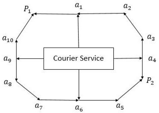
Figure 1. Traffic network pattern with 6 routes, i.e., $p=6$.

We have explicitly $p=6$ paths in the given traffic network. The courier company must find the entire traffic flow vector to minimize the cost of each route $\{r_1,r_2,r_3,r_4,r_5,r_6\}$. This can be calculated by solving the multi-time optimization problem (10).

5.2. River Basin Pollution Problem

In this subsection we show how our multi-time generalized Nash equilibrium problem can be applied to solving the river basin pollution problem [38]. For studies of the river basin pollution problem, we refer the interested reader to [39,40,41]. We use the term time $t\in {\mathrm{\Omega }}_{l_{\circ },l_1}$ as defined in Section 2. We assume that n industrial factories (paper mills, chemical factories, pharmaceutical manufacturing companies, etc.) are located along a river. In the sequel we call them industrial agents. Presently, it is a very common scenario that industrial factories often dump waste garbage, such as dirty water, used chemicals and oils, sewage, and cafeteria waste, directly into a community water source (river, lake or stream). Waste dumped contains several contaminants which mix and create pollution concentration along the river. We assume that m basin authorities (monitoring stations) are located along the river. Each basin authority is empowered to set a maximum pollutant concentration level at time t which we denote by ${\chi }_s\left(t\right)\in L^2({\mathrm{\Omega }}_{l_{\circ },l_1},{\mathbb{R}}_{+})$ where $s\in \{1,2,\dots ,m\}$. Furthermore, we let $e^f\left(t\right)\in L^2({\mathrm{\Omega }}_{l_{\circ },l_1},{\mathbb{R}}_{+})$ be the pollutant emission coefficient for the industrial agent $f\in \{1,2,\dots ,n\}$. Let $x^f\left(t\right)\in L^2({\mathrm{\Omega }}_{l_{\circ },l_1},{\mathbb{R}}_{+})$ be the chosen emitted pollutant concentration level at time t by the industrial agent f and let $x^{-f}\left(t\right)\in L^2({\mathrm{\Omega }}_{l_{\circ },l_1},{\mathbb{R}}_{+}^{n-1})$ be the chosen emitted pollutant concentration level at time t by all the industrial agents except the agent f. Furthermore, let $x\left(t\right)\in L^2({\mathrm{\Omega }}_{l_{\circ },l_1},{\mathbb{R}}_{+}^n)$ be the chosen emitted pollutant concentration level at time t by all the industrial agents. To put the chosen emitted pollutant concentration level $x^f\left(t\right)$ of the industrial agent f in focus, we write $x\left(t\right)$ as $x\left(t\right)=(x^f\left(t\right),x^{-f}\left(t\right))$. Please note that $x\left(t\right)$ is still the vector $x\left(t\right)=(x^1\left(t\right),x^2\left(t\right),\dots ,x^{f-1}\left(t\right),x^f\left(t\right),x^{f+1}\left(t\right),\dots ,x^n\left(t\right))$. Waste materials, dumped by the industrial agents into the river, spread, decay and then finally reach the basin authorities. Thus, the amount of pollution received by the basin authority $s\in \{1,2,\dots ,m\}$ is ${\displaystyle \sum _{f=1}^n}{\delta }_s^f\left(t\right)e^f\left(t\right)x^f\left(t\right)$, where ${\delta }_s^f\left(t\right)$ is the decay-and-transportation coefficient from the agent f to the monitoring station s. The basin authorities impose constraints on the pollution, so that industrial agents control their pollutant emission into the river. Thus, the pollution constraint set imposed by the authority s is given by

$${\displaystyle \sum _{f=1}^n}{\delta }_s^f\left(t\right)e^f\left(t\right)x^f\left(t\right)\le {\chi }_s\left(t\right)\mathrm{for}s\in \{1,2,\dots ,m\}\mathrm{and}\mathrm{a}.\mathrm{e}.\mathrm{on}{\mathrm{\Omega }}_{l_{\circ },l_1}.$$

The nonempty set of entire feasible pollution concentration levels is given by

$$K=\{x\left(t\right)\in L^2({\mathrm{\Omega }}_{l_{\circ },l_1},{\mathbb{R}}_{+}^n):{\displaystyle \sum _{f=1}^n}{\delta }_s^f\left(t\right)e^f\left(t\right)x^f\left(t\right)\le {\chi }_s\left(t\right)\mathrm{for}s\in \{1,2,\dots ,m\}$$

$$\mathrm{and}\mathrm{a}.\mathrm{e}.\mathrm{on}{\mathrm{\Omega }}_{l_{\circ },l_1}\}.$$

We bear in the mind that industrial agents are dependent on each other, at least because of the finiteness of the amount of dumping pollutants into the river. Therefore, for any given $x^{-f}\left(t\right)$, the nonempty, closed and convex feasible pollution concentration level set of each industrial agent f is denoted by $K_f\left(x^{-f}\left(t\right)\right)$. This is a subset of $L^2({\mathrm{\Omega }}_{l_{\circ },l_1},{\mathbb{R}}_{+})$. Each agent wishes to maximize its profit in the time period t, where the profit is defined by the difference between the revenue $[p_1-p_2{\displaystyle \sum _{f=1}^n}{x}^f\left(t\right)]x^f\left(t\right)$ and the cost $[a^f\left(t\right)+b^f\left(t\right)x^f\left(t\right)]x^f\left(t\right)$. Here $p_1$ and $p_2$ are economic constants which follow the inverse demand law and $a^f\left(t\right),b^f\left(t\right)\in L^2({\mathrm{\Omega }}_{l_{\circ },l_1},{\mathbb{R}}_{+})$ are the cost coefficient functions. Now, for a given $x^{-f}\left(t\right)$, the aim of the industrial agent f is to choose an emitted pollutant concentration level $x^f\left(t\right)$ such that it solves the following multi-time maximization problem:

$$\underset{x^f\left(t\right)}{max}{\int }_{{\mathrm{\Omega }}_{l_{\circ },l_1}}\left[\left\{\left(p_1-p_2{\displaystyle \sum _{f=1}^n}{x}^f\left(t\right)\right)x^f\left(t\right)\right\}-\left\{(a^f\left(t\right)+b^f\left(t\right)x^f\left(t\right))x^f\left(t\right)\right\}\right]dt,$$

$$\mathrm{subject}\mathrm{to}{x}^f\left(t\right)\in K_f\left(x^{-f}\left(t\right)\right).$$

An equilibrium of the above defined multi-time maximization problem is a multi-time generalized Nash equilibrium in the sense of our (MGNEP), where

$$f^{\mu }(x^{\mu }\left(t\right),x^{-\mu }\left(t\right))=\left[\left\{(a^{\mu }\left(t\right)+b^{\mu }\left(t\right)x^{\mu }\left(t\right))x^{\mu }\left(t\right)\right\}-\left\{\left(p_1-p_2{\displaystyle \sum _{\mu =1}^n}{x}^{\mu }\left(t\right)\right)x^{\mu }\left(t\right)\right\}\right].$$

6. The Multi-Time Generalized Nash Equilibrium Problem as a Projected Dynamical  System

In this section, we investigate our multi-time generalized Nash equilibrium problem via a projected dynamical system. We also propose a method for finding the equilibria of our multi-time generalized Nash equilibrium problem. Our work is motivated by [12,20,42]. We also refer the interested reader to the more recent work [29], which deals with a projected dynamical system pertaining to a single-valued map in the context of a multi-time variational inequality problem, while the projected dynamical system of this section pertains to a set-valued map in the context of a multi-time quasi-variational inequality problem. More precisely, in the present section we consider the following projected dynamical system (PDS) pertaining to the set-valued map $\mathrm{\Gamma }$, where $x(·)\in \mathrm{\Gamma }\left(x\right(·\left)\right)$:

$$\begin{array}{l}\frac{dx(·,\tau )}{d\tau }={\mathrm{\Pi }}_{\mathrm{\Gamma }\left(x\right(·,\tau \left)\right)}(x(·,\tau ),-J\left(x(·,\tau )\right)),\\ x(·,0)=x_{\circ }(·)\in \mathrm{\Gamma }\left(x(·)\right),\end{array}$$

(11)

where $J:L^2({\mathrm{\Omega }}_{l_{\circ },l_1},{\mathbb{R}}^n)\to L^2({\mathrm{\Omega }}_{l_{\circ },l_1},{\mathbb{R}}^n)$ is a Lipschitz continuous vector field and ${\mathrm{\Pi }}_{\mathrm{\Gamma }\left(x\right(·\left)\right)}:L^2({\mathrm{\Omega }}_{l_{\circ },l_1},{\mathbb{R}}^n)\times L^2({\mathrm{\Omega }}_{l_{\circ },l_1},{\mathbb{R}}^n)\to L^2({\mathrm{\Omega }}_{l_{\circ },l_1},{\mathbb{R}}^n)$ is the operator defined by

$${\mathrm{\Pi }}_{\mathrm{\Gamma }\left(x\right(·\left)\right)}(x(·),v(·)):=\underset{\delta \to 0^{+}}{lim}\frac{{\mathrm{proj}}_{\mathrm{\Gamma }\left(x\right(·\left)\right)}(x(·)+\delta v(·))-x(·)}{\delta },$$

where $x(·)\in K\mathrm{and}v(·)\in L^2({\mathrm{\Omega }}_{l_{\circ },l_1},{\mathbb{R}}^n)$. The characteristics of the times t and $\tau$ in (PDS) are different. Indeed, for all $t\in {\mathrm{\Omega }}_{l_{\circ },l_1}$, a solution of (MQVIP) specifies the static states of the underlying system and the static states defined by one or more equilibrium curves when t varies over the set ${\mathrm{\Omega }}_{l_{\circ },l_1}$. On the other hand, $\tau$ represents the dynamics of the system over the interval $[0,\infty )$ until it reaches one of the equilibria on the curves. It is evident that the solutions of (PDS) lie in the class of absolutely continuous functions with respect to $\tau$, which take $[0,\infty )$ into $\mathrm{\Gamma }\left(x\right(·\left)\right)$. Moreover, to avoid any possible confusion between t and $\tau$, we represent elements of the sets $L^2({\mathrm{\Omega }}_{l_{\circ },l_1},{\mathbb{R}}^n)$ at fixed moments $t\in {\mathrm{\Omega }}_{l_{\circ },l_1}$ by $x(·)$. To describe the connection of our (MGNEP) with (PDS), we need the following definition, which is inspired by [42].

Definition 9.

$y(·)\in K$ is called a critical point of (PDS) if $y(·)\in \mathrm{\Gamma }\left(y\right(·\left)\right)$ and

$${\mathrm{\Pi }}_{\mathrm{\Gamma }\left(y\right(·\left)\right)}(y(·),-J\left(y(·)\right))=0.$$

Lemma 1

([43], Lemma 1.2.8). For each $i=\{1,2,\dots ,p\}$, let $H_i$ be a Hilbert space and let $C_i\subset H_i$ be closed and convex, Set $C=C_1\times C_2\times \dots \times C_p\subset H_1\times H_2\times \dots \times H_p=H$ and let $x=(x_1,x_2,\dots ,x_p)\in H$. Let $pro{j}_{C_i}$ denote the metric projection onto $C_i$. Then the metric projection ${\mathit{proj}}_C\left(x\right)$ is given by

$${\mathit{proj}}_C\left(x\right)=({\mathit{proj}}_{C_1}\left(x_1\right),{\mathit{proj}}_{C_2}\left(x_2\right),\dots ,{\mathit{proj}}_{C_p}\left(x_p\right)).$$

The following propositions concerning each player $\mu \in \{1,2,\dots ,N\}$ and the strategies $y^{-\mu }(·)\in L^2({\mathrm{\Omega }}_{l_{\circ },l_1},{\mathbb{R}}^{n-n_{\mu }})$ of the rival players except player $\mu$ are direct consequences of Proposition $2.1$ and $2.2$ in [42].

Proposition 1.

For all $y^{\mu }(·)\in K_{\mu }\left(y^{-\mu }(·)\right)$ and $v^{\mu }(·)\in L^2({\mathrm{\Omega }}_{l_{\circ },l_1},{\mathbb{R}}^{n_{\mu }})$,${\mathrm{\Pi }}_{K_{\mu }\left(y^{-\mu }(·)\right)}(y^{\mu }(·),v^{\mu }(·))$ exists and ${\mathrm{\Pi }}_{K_{\mu }\left(y^{-\mu }(·)\right)}(y^{\mu }(·),v^{\mu }(·))={\mathit{proj}}_{T_{K_{\mu }\left(y^{-\mu }(·)\right)}\left(y^{\mu }(·)\right)}\left(v^{\mu }(·)\right)$.

Proposition 2.

For each $y^{\mu }(·)\in K_{\mu }\left(y^{-\mu }(·)\right)$, there exists $n^{\mu }(·)\in N_{K_{\mu }\left(y^{-\mu }(·)\right)}\left(y^{\mu }(·)\right)$ such that ${\mathrm{\Pi }}_{K_{\mu }\left(y^{-\mu }(·)\right)}(y^{\mu }(·),v^{\mu }(·))=v^{\mu }(·)-n^{\mu }(·)\mathit{for}\mathit{all}{v}^{\mu }(·)\in L^2({\mathrm{\Omega }}_{l_{\circ },l_1},{\mathbb{R}}^{n_{\mu }})$.

The following theorem establishes a strong connection between (MGNEP) and (PDS).

Theorem 4.

Assume that $J\left(x(·)\right)={\left(\frac{\partial f^{\mu }}{\partial x^{\mu }}\left(x(·)\right)\right)}_{\mu =1}^N$ for any $x(·)\in K$, and that for each $\mu \in \{1,2,\dots ,N\}$ and $x^{-\mu }(·)$, the multi-time cost functional $F^{\mu }$ is convex on K in the argument $x^{\mu }(·)$. Then $y(·)\in K$ is a multi-time generalized Nash equilibrium if and only if it is a critical point of (PDS).

Proof. 

Suppose that $y(·)\in K$ is a multi-time generalized Nash equilibrium. Then it follows from Theorem 2 that for each $\mu \in \{1,2,\dots ,N\}$, we have

$${\int }_{{\mathrm{\Omega }}_{l_{\circ },l_1}}⟨\frac{\partial f^{\mu }}{\partial x^{\mu }}\left(y(·)\right),x^{\mu }(·)-y^{\mu }(·)⟩dt\ge 0\forall x^{\mu }(·)\in K_{\mu }\left(y^{-\mu }(·)\right).$$

The above inequality can be rewritten as

$$⟨⟨\frac{\partial f^{\mu }}{\partial x^{\mu }}\left(y(·)\right),x^{\mu }(·)-y^{\mu }(·)⟩⟩\ge 0\forall x^{\mu }(·)\in K_{\mu }\left(y^{-\mu }(·)\right),$$

which leads to the following inclusion:

$$-\frac{\partial f^{\mu }}{\partial x^{\mu }}\left(y(·)\right)\in N_{K_{\mu }\left(y^{-\mu }(·)\right)}\left(y^{\mu }(·)\right).$$

Proposition 2 now yields

$${\mathrm{\Pi }}_{K_{\mu }\left(y^{-\mu }(·)\right)}\left(y^{\mu }(·),-\frac{\partial f^{\mu }}{\partial x^{\mu }}\left(y(·)\right)\right)=0.$$

(12)

Since $K_{\mu }\left(y^{-\mu }(·)\right)$ is convex for each $\mu \in \{1,2,\dots ,N\}$, Lemma 1 implies that

$${\mathrm{\Pi }}_{\mathrm{\Gamma }\left(y\right(·\left)\right)}(y(·),-J\left(y(·)\right))=0.$$

(13)

Therefore $y(·)$ is indeed a critical point of (PDS), as asserted.

Conversely, assume that $y(·)\in K$ is a critical point of (PDS). Then $y(·)\in \mathrm{\Gamma }\left(y\right(·\left)\right)$ and inequality (13) holds. Consequently, (12) holds too. Proposition 1 implies that

$${\mathrm{proj}}_{T_{K_{\mu }\left(y^{-\mu }(·)\right)}\left(y^{\mu }(·)\right)}\left(-\frac{\partial f^{\mu }}{\partial x^{\mu }}\left(y(·)\right)\right)=0.$$

In view of Remark 2, the above expression leads to

$$⟨⟨-\frac{\partial f^{\mu }}{\partial x^{\mu }}\left(y(·)\right),z^{\mu }(·)⟩⟩\le 0\forall z^{\mu }(·)\in T_{K_{\mu }\left(y^{-\mu }(·)\right)}\left(y^{\mu }(·)\right),$$

which in turn implies that

$$-\frac{\partial f^{\mu }}{\partial x^{\mu }}\left(y(·)\right)\in N_{K_{\mu }\left(y^{-\mu }(·)\right)}\left(y^{\mu }(·)\right),$$

which yields that $y(·)$ is a solution of (MQVIP) with $J\left(y(·)\right)={\left(\frac{\partial f^{\mu }}{\partial x^{\mu }}\left(y(·)\right)\right)}_{\mu =1}^N$. Thus, the first part of the proof of Theorem 2 implies that $y(·)$ is a multi-time generalized Nash equilibrium. □

Remark 5.

In view of the proof techniques of Theorem 4 and the fact that the normal cone of a product set is equal to the product of the normal cones ([44], Proposition 6.41), we can write (PDS) (11) as a concatenation of the following N dynamical systems (PDS)${}_{\mu }$ for $J\left(x(·,\tau )\right)={\left(\frac{\partial f^{\mu }}{\partial x^{\mu }}\left(x(·,\tau )\right)\right)}_{\mu =1}^N$:

$$\begin{array}{c}\frac{d{x}^{\mu }(·,\tau )}{d\tau }={\mathrm{\Pi }}_{K_{\mu }\left(x^{-\mu }(·,\tau )\right)}\left(x^{\mu }(·,\tau ),-\frac{\partial f^{\mu }}{\partial x^{\mu }}\left(x(·,\tau )\right)\right),\\ x^{\mu }(·,0)=x_{\circ }^{\mu }(·)\in K_{\mu }\left(x^{-\mu }(·)\right).\end{array}$$

Numerical Illustrations

In this subsection we turn our attention to demonstrating a method for solving (MGNEP) by taking advantage of (PDS) (11). Theorem 4 tells us that any point on a curve of equilibria in the set K is a critical point of (PDS) and vice versa. Please note that the existence of equilibria has already been established. Next, we take the following discretization of ${\mathrm{\Omega }}_{l_{\circ },l_1}$: $(l_{\circ }^1,l_{\circ }^2,\dots ,l_{\circ }^m)=(t_{\circ }^1,t_{\circ }^2,\dots ,t_{\circ }^m)<(t_1^1,t_1^2,\dots ,t_1^m)<\dots <(t_i^1,t_i^2,\dots ,t_i^m)<\dots <(t_n^1,t_n^2,\dots ,t_n^m)$$=(l_1^1,l_1^2,\dots ,l_1^m)$. Then for each $t_i=(t_i^1,t_i^2,\dots ,t_i^m),i=\{0,1,\dots ,n\}$, we obtain a sequence of (PDS) on the distinct, nonempty, finite-dimensional and convex sets $K_{t_i}$. After computing all the critical points of each (PDS), we obtain a sequence of critical points which by interpolation yields the curves of equilibria. To apply this procedure in practice, we consider a Nguyen traffic network [31] which comprises 13 nodes, 19 links, four origin–destination pairs and 24 paths. See Figure 2. Here we use the terminology of Section 5. Every origin–destination pair of our Nguyen traffic network is connected by six paths. Let $m=2$ and ${\mathrm{\Omega }}_{l_{\circ },l_1}={\mathrm{\Omega }}_{0,4}={[0,4]}^2$. The set of feasible flows is given by

$$K=\{x\left(t\right)\in L^2({\mathrm{\Omega }}_{0,4},{\mathbb{R}}_{+}^{24}):(0,\dots ,0)\le {\left(x^r\left(t\right)\right)}_{r=1}^{24}\le {(t^1+t^2+r)}_{r=1}^{24}$$

$$\mathrm{and}\sum _{r=1}^6{x}^r\left(t\right)=6t^1+6t^2+21,\sum _{r=7}^{12}{x}^r\left(t\right)=6t^1+6t^2+57,$$

$$\sum _{r=13}^{18}{x}^r\left(t\right)=6t^1+6t^2+93,\sum _{r=19}^{24}{x}^r\left(t\right)=6t^1+6t^2+129\mathrm{a}.\mathrm{e}.\mathrm{on}{\mathrm{\Omega }}_{0,4}\}.$$

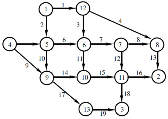
Figure 2. The Nguyen traffic network (13 nodes, 19 links, 4 origin–destination pairs).

To simplify our calculations, we assume the following special structure of the feasible traffic flow set of each route $r\in \{1,2,\dots ,24\}$. This is motivated by Rosen [5].

$$K_r\left(x^{-r}\left(t\right)\right)=\{x\left(t\right)\in L^2({\mathrm{\Omega }}_{0,4},{\mathbb{R}}_{+}):(x^r\left(t\right),x^{-r}\left(t\right))\in K\}$$

and the multi-time cost functional of each route $r\in \{1,2,\dots ,24\}$ is defined by

$$H^r\left(x\left(t\right)\right)={\int }_{{\mathrm{\Omega }}_{0,4}}(x^r\left(s\right)+{\left(x^r\left(s\right)\right)}^2)ds,$$

where $x\left(t\right)=(x^1\left(t\right),x^2\left(t\right),\dots ,x^{r-1}\left(t\right),x^r\left(t\right),x^{r+1}\left(t\right),\dots ,x^{24}\left(t\right))$. It can easily be proven that for each $r\in \{1,2,\dots ,24\}$, the multi-time cost functional $H^r\left(x\left(t\right)\right)$ is convex in the argument $x^r\left(t\right)$ and that there exists a nonempty, closed and compact subset $D\subset K$ which is given by

$$D=\{x\left(t\right)\in L^2({\mathrm{\Omega }}_{0,4},{\mathbb{R}}_{+}^{24}):(0,\dots ,0)\le {\left(x^r\left(t\right)\right)}_{r=1}^{24}\le {\left(t^1+t^2+\frac{r}{2}\right)}_{r=1}^{24}$$

$$\mathrm{and}\sum _{r=1}^6{x}^r\left(t\right)=6t^1+6t^2+21,\sum _{r=7}^{12}{x}^r\left(t\right)=6t^1+6t^2+57,$$

$$\sum _{r=13}^{18}{x}^r\left(t\right)=6t^1+6t^2+93,\sum _{r=19}^{24}{x}^r\left(t\right)=6t^1+6t^2+129\mathrm{a}.\mathrm{e}.\mathrm{on}{\mathrm{\Omega }}_{0,4}\}$$

such that for $\widehat{y}\left(t\right)\in D$, inequality (6) is satisfied. Thus, all the hypotheses of Theorem 3 are fulfilled. Therefore, for $J\left(y\left(t\right)\right)={(1+2y^r\left(t\right))}_{r=1}^{24}$, (MDVIP) has a solution. Consequently, by Theorem 2, (MGNEP) has a solution too.

Selecting points $t_i\in \left\{\left(\frac{k}{8},\frac{k}{8}\right):k\in \{0,1,2,\dots ,32\}\right\}$, we obtain a sequence of (PDS) defined on the sets

$$K_{t_i}=\{x\left(t_i\right)\in L^2({\mathrm{\Omega }}_{0,4},{\mathbb{R}}_{+}^{24}):(0,\dots ,0)\le {\left(x^r\left(t_i\right)\right)}_{r=1}^{24}\le {(t_i^1+t_i^2+r)}_{r=1}^{24}$$

$$\mathrm{and}\sum _{r=1}^6{x}^r\left(t_i\right)=6t_i^1+6t_i^2+21,\sum _{r=7}^{12}{x}^r\left(t_i\right)=6t_i^1+6t_i^2+57,$$

$$\sum _{r=13}^{18}{x}^r\left(t_i\right)=6t_i^1+6t_i^2+93,\sum _{r=19}^{24}{x}^r\left(t_i\right)=6t_i^1+6t_i^2+129\mathrm{a}.\mathrm{e}.\mathrm{on}{\mathrm{\Omega }}_{0,4}\}.$$

We have

$$K_r\left(x^{-r}\left(t_i\right)\right)=\{x\left(t_i\right)\in L^2({\mathrm{\Omega }}_{0,4},{\mathbb{R}}_{+}):(x^r\left(t_i\right),x^{-r}\left(t_i\right))\in K_{t_i}\},$$

$$\mathrm{and}\mathrm{\Gamma }\left(y\left(t_i\right)\right)=\prod _{r=1}^{24}{K}_r\left(y^{-r}\left(t_i\right)\right).$$

For calculating the equilibrium, we consider the following system at the points $t_i$: to find the point $y\left(t_i\right)=(y^1\left(t_i\right),y^2\left(t_i\right),\dots ,y^{r-1}\left(t_i\right),y^r\left(t_i\right),y^{r+1}\left(t_i\right),\dots ,y^{24}\left(t_i\right))\in K_{t_i}$ such that

$$-(1+2y^r\left(t_i\right))\in N_{K_r\left(y^{-r}\left(t_i\right)\right)}\left(y^r\left(t_i\right)\right).$$

After a simple calculation, we find the equilibrium points which are given in Table 1, Table 2, Table 3 and Table 4. We then interpolate the points of these tables and finally obtain the curves of equilibria. They are displayed in Figure 3.

Table 1. Numerical Results.

${\mathit{t}}_{\mathit{i}}=\{{\mathit{t}}_{\mathit{i}}^1,{\mathit{t}}_{\mathit{i}}^2\}$	${\mathit{y}}^1\left({\mathit{t}}_{\mathit{i}}\right)$	${\mathit{y}}^2\left({\mathit{t}}_{\mathit{i}}\right)$	${\mathit{y}}^3\left({\mathit{t}}_{\mathit{i}}\right)$	${\mathit{y}}^4\left({\mathit{t}}_{\mathit{i}}\right)$	${\mathit{y}}^5\left({\mathit{t}}_{\mathit{i}}\right)$	${\mathit{y}}^6\left({\mathit{t}}_{\mathit{i}}\right)$
$\{0,0\}$	1	2	3	4	5	6
$\{\frac{1}{8},\frac{1}{8}\}$	1.25	2.25	3.25	4.25	5.25	6.25
$\{\frac{1}{4},\frac{1}{4}\}$	1.5	2.5	3.5	4.5	5.5	6.5
$\{\frac{3}{8},\frac{3}{8}\}$	1.75	2.75	3.75	4.75	5.75	6.75
$\{\frac{1}{2},\frac{1}{2}\}$	2	3	4	5	6	7
$\{\frac{5}{8},\frac{5}{8}\}$	2.25	3.25	4.25	5.25	6.25	7.25
$\{\frac{3}{4},\frac{3}{4}\}$	2.5	3.5	4.5	5.5	6.5	7.5
$\{\frac{7}{8},\frac{7}{8}\}$	2.75	3.75	4.75	5.75	6.75	7.75
$\{1,1\}$	3	4	5	6	7	8
$\{\frac{9}{8},\frac{9}{8}\}$	3.25	4.25	5.25	6.25	7.25	8.25
$\{\frac{5}{4},\frac{5}{4}\}$	3.5	4.5	5.5	6.5	7.5	8.5
$\{\frac{11}{8},\frac{11}{8}\}$	3.75	4.75	5.75	6.75	7.75	8.75
$\{\frac{3}{2},\frac{3}{2}\}$	4	5	6	7	8	9
$\{\frac{13}{8},\frac{13}{8}\}$	4.25	5.25	6.25	7.25	8.25	9.25
$\{\frac{7}{4},\frac{7}{4}\}$	4.5	5.5	6.5	7.5	8.5	9.5
$\{\frac{15}{8},\frac{15}{8}\}$	4.75	5.75	6.75	7.75	8.75	9.75
$\{2,2\}$	5	6	7	8	9	10
$\{\frac{17}{8},\frac{17}{8}\}$	5.25	6.25	7.25	8.25	9.25	10.25
$\{\frac{9}{4},\frac{9}{4}\}$	5.5	6.5	7.5	8.5	9.5	10.5
$\{\frac{19}{8},\frac{19}{8}\}$	5.75	6.75	7.75	8.75	9.75	10.75
$\{\frac{5}{2},\frac{5}{2}\}$	6	7	8	9	10	11
$\{\frac{21}{8},\frac{21}{8}\}$	6.25	7.25	8.25	9.25	10.25	11.25
$\{\frac{11}{4},\frac{11}{4}\}$	6.5	7.5	8.5	9.5	10.5	11.5
$\{\frac{23}{8},\frac{23}{8}\}$	6.75	7.75	8.75	9.75	10.75	11.75
$\{3,3\}$	7	8	9	10	11	12
$\{\frac{25}{8},\frac{25}{8}\}$	7.25	8.25	9.25	10.25	11.25	12.25
$\{\frac{13}{4},\frac{13}{4}\}$	7.5	8.5	9.5	10.5	11.5	12.5
$\{\frac{27}{8},\frac{27}{8}\}$	7.75	8.75	9.75	10.75	11.75	12.75
$\{\frac{7}{2},\frac{7}{2}\}$	8	9	10	11	12	13
$\{\frac{29}{8},\frac{29}{8}\}$	8.25	9.25	10.25	11.25	12.25	13.25
$\{\frac{15}{4},\frac{15}{4}\}$	8.5	9.5	10.5	11.5	12.5	13.5
$\{\frac{31}{8},\frac{31}{8}\}$	8.75	9.75	10.75	11.75	12.75	13.75
$\{4,4\}$	9	10	11	12	13	14

Table 2. Numerical Results.

${\mathit{t}}_{\mathit{i}}=\{{\mathit{t}}_{\mathit{i}}^1,{\mathit{t}}_{\mathit{i}}^2\}$	${\mathit{y}}^7\left({\mathit{t}}_{\mathit{i}}\right)$	${\mathit{y}}^8\left({\mathit{t}}_{\mathit{i}}\right)$	${\mathit{y}}^9\left({\mathit{t}}_{\mathit{i}}\right)$	${\mathit{y}}^{10}\left({\mathit{t}}_{\mathit{i}}\right)$	${\mathit{y}}^{11}\left({\mathit{t}}_{\mathit{i}}\right)$	${\mathit{y}}^{12}\left({\mathit{t}}_{\mathit{i}}\right)$
$\{0,0\}$	7	8	9	10	11	12
$\{\frac{1}{8},\frac{1}{8}\}$	7.25	8.25	9.25	10.25	11.25	12.25
$\{\frac{1}{4},\frac{1}{4}\}$	7.5	8.5	9.5	10.5	11.5	12.5
$\{\frac{3}{8},\frac{3}{8}\}$	7.75	8.75	9.75	10.75	11.75	12.75
$\{\frac{1}{2},\frac{1}{2}\}$	8	9	10	11	12	13
$\{\frac{5}{8},\frac{5}{8}\}$	8.25	9.25	10.25	11.25	12.25	13.25
$\{\frac{3}{4},\frac{3}{4}\}$	8.5	9.5	10.5	11.5	12.5	13.5
$\{\frac{7}{8},\frac{7}{8}\}$	8.75	9.75	10.75	11.75	12.75	13.75
$\{1,1\}$	9	10	11	12	13	14
$\{\frac{9}{8},\frac{9}{8}\}$	9.25	10.25	11.25	12.25	13.25	14.25
$\{\frac{5}{4},\frac{5}{4}\}$	9.5	10.5	11.5	12.5	13.5	14.5
$\{\frac{11}{8},\frac{11}{8}\}$	9.75	10.75	11.75	12.75	13.75	14.75
$\{\frac{3}{2},\frac{3}{2}\}$	10	11	12	13	14	15
$\{\frac{13}{8},\frac{13}{8}\}$	10.25	11.25	12.25	13.25	14.25	15.25
$\{\frac{7}{4},\frac{7}{4}\}$	10.5	11.5	12.5	13.5	14.5	15.5
$\{\frac{15}{8},\frac{15}{8}\}$	10.75	11.75	12.75	13.75	14.75	15.75
$\{2,2\}$	11	12	13	14	15	16
$\{\frac{17}{8},\frac{17}{8}\}$	11.25	12.25	13.25	14.25	15.25	16.25
$\{\frac{9}{4},\frac{9}{4}\}$	11.5	12.5	13.5	14.5	15.5	16.5
$\{\frac{19}{8},\frac{19}{8}\}$	11.75	12.75	13.75	14.75	15.75	16.75
$\{\frac{5}{2},\frac{5}{2}\}$	12	13	14	15	16	17
$\{\frac{21}{8},\frac{21}{8}\}$	12.25	13.25	14.25	15.25	16.25	17.25
$\{\frac{11}{4},\frac{11}{4}\}$	12.5	13.5	14.5	15.5	16.5	17.5
$\{\frac{23}{8},\frac{23}{8}\}$	12.75	13.75	14.75	15.75	16.75	17.75
$\{3,3\}$	13	14	15	16	17	18
$\{\frac{25}{8},\frac{25}{8}\}$	13.25	14.25	15.25	16.25	17.25	18.25
$\{\frac{13}{4},\frac{13}{4}\}$	13.5	14.5	15.5	16.5	17.5	18.5
$\{\frac{27}{8},\frac{27}{8}\}$	13.75	14.75	15.75	16.75	17.75	18.75
$\{\frac{7}{2},\frac{7}{2}\}$	14	15	16	17	18	19
$\{\frac{29}{8},\frac{29}{8}\}$	14.25	15.25	16.25	17.25	18.25	19.25
$\{\frac{15}{4},\frac{15}{4}\}$	14.5	15.5	16.5	17.5	18.5	19.5
$\{\frac{31}{8},\frac{31}{8}\}$	14.75	15.75	16.75	17.75	18.75	19.75
$\{4,4\}$	15	16	17	18	19	20

Table 3. Numerical Results.

${\mathit{t}}_{\mathit{i}}=\{{\mathit{t}}_{\mathit{i}}^1,{\mathit{t}}_{\mathit{i}}^2\}$	${\mathit{y}}^{13}\left({\mathit{t}}_{\mathit{i}}\right)$	${\mathit{y}}^{14}\left({\mathit{t}}_{\mathit{i}}\right)$	${\mathit{y}}^{15}\left({\mathit{t}}_{\mathit{i}}\right)$	${\mathit{y}}^{16}\left({\mathit{t}}_{\mathit{i}}\right)$	${\mathit{y}}^{17}\left({\mathit{t}}_{\mathit{i}}\right)$	${\mathit{y}}^{18}\left({\mathit{t}}_{\mathit{i}}\right)$
$\{0,0\}$	13	14	15	16	17	18
$\{\frac{1}{8},\frac{1}{8}\}$	13.25	14.25	15.25	16.25	17.25	18.25
$\{\frac{1}{4},\frac{1}{4}\}$	13.5	14.5	15.5	16.5	17.5	18.5
$\{\frac{3}{8},\frac{3}{8}\}$	13.75	14.75	15.75	16.75	17.75	18.75
$\{\frac{1}{2},\frac{1}{2}\}$	14	15	16	17	18	19
$\{\frac{5}{8},\frac{5}{8}\}$	14.25	15.25	16.25	17.25	18.25	19.25
$\{\frac{3}{4},\frac{3}{4}\}$	14.5	15.5	16.5	17.5	18.5	19.5
$\{\frac{7}{8},\frac{7}{8}\}$	14.75	15.75	16.75	17.75	18.75	19.75
$\{1,1\}$	15	16	17	18	19	20
$\{\frac{9}{8},\frac{9}{8}\}$	15.25	16.25	17.25	18.25	19.25	20.25
$\{\frac{5}{4},\frac{5}{4}\}$	15.5	16.5	17.5	18.5	19.5	20.5
$\{\frac{11}{8},\frac{11}{8}\}$	15.75	16.75	17.75	18.75	19.75	20.75
$\{\frac{3}{2},\frac{3}{2}\}$	16	17	18	19	20	21
$\{\frac{13}{8},\frac{13}{8}\}$	16.25	17.25	18.25	19.25	20.25	21.25
$\{\frac{7}{4},\frac{7}{4}\}$	16.5	17.5	18.5	19.5	20.5	21.5
$\{\frac{15}{8},\frac{15}{8}\}$	16.75	17.75	18.75	19.75	20.75	21.75
$\{2,2\}$	17	18	19	20	21	22
$\{\frac{17}{8},\frac{17}{8}\}$	17.25	18.25	19.25	20.25	21.25	22.25
$\{\frac{9}{4},\frac{9}{4}\}$	17.5	18.5	19.5	20.5	21.5	22.5
$\{\frac{19}{8},\frac{19}{8}\}$	17.75	18.75	19.75	20.75	21.75	22.75
$\{\frac{5}{2},\frac{5}{2}\}$	18	19	20	21	22	23
$\{\frac{21}{8},\frac{21}{8}\}$	18.25	19.25	20.25	21.25	22.25	23.25
$\{\frac{11}{4},\frac{11}{4}\}$	18.5	19.5	20.5	21.5	22.5	23.5
$\{\frac{23}{8},\frac{23}{8}\}$	18.75	19.75	20.75	21.75	22.75	23.75
$\{3,3\}$	19	20	21	22	23	24
$\{\frac{25}{8},\frac{25}{8}\}$	19.25	20.25	21.25	22.25	23.25	24.25
$\{\frac{13}{4},\frac{13}{4}\}$	19.5	20.5	21.5	22.5	23.5	24.5
$\{\frac{27}{8},\frac{27}{8}\}$	19.75	20.75	21.75	22.75	23.75	24.75
$\{\frac{7}{2},\frac{7}{2}\}$	20	21	22	23	24	25
$\{\frac{29}{8},\frac{29}{8}\}$	20.25	21.25	22.25	23.25	24.25	25.25
$\{\frac{15}{4},\frac{15}{4}\}$	20.5	21.5	22.5	23.5	24.5	25.5
$\{\frac{31}{8},\frac{31}{8}\}$	20.75	21.75	22.75	23.75	24.75	25.75
$\{4,4\}$	21	22	23	24	25	26

Table 4. Numerical Results.

${\mathit{t}}_{\mathit{i}}=\{{\mathit{t}}_{\mathit{i}}^1,{\mathit{t}}_{\mathit{i}}^2\}$	${\mathit{y}}^{19}\left({\mathit{t}}_{\mathit{i}}\right)$	${\mathit{y}}^{20}\left({\mathit{t}}_{\mathit{i}}\right)$	${\mathit{y}}^{21}\left({\mathit{t}}_{\mathit{i}}\right)$	${\mathit{y}}^{22}\left({\mathit{t}}_{\mathit{i}}\right)$	${\mathit{y}}^{23}\left({\mathit{t}}_{\mathit{i}}\right)$	${\mathit{y}}^{24}\left({\mathit{t}}_{\mathit{i}}\right)$
$\{0,0\}$	19	20	21	22	23	24
$\{\frac{1}{8},\frac{1}{8}\}$	19.25	20.25	21.25	22.25	23.25	24.25
$\{\frac{1}{4},\frac{1}{4}\}$	19.5	20.5	21.5	22.5	23.5	24.5
$\{\frac{3}{8},\frac{3}{8}\}$	19.75	20.75	21.75	22.75	23.75	24.75
$\{\frac{1}{2},\frac{1}{2}\}$	20	21	22	23	24	25
$\{\frac{5}{8},\frac{5}{8}\}$	20.25	21.25	22.25	23.25	24.25	25.25
$\{\frac{3}{4},\frac{3}{4}\}$	20.5	21.5	22.5	23.5	24.5	25.5
$\{\frac{7}{8},\frac{7}{8}\}$	20.75	21.75	22.75	23.75	24.75	25.75
$\{1,1\}$	21	22	23	24	25	26
$\{\frac{9}{8},\frac{9}{8}\}$	21.25	22.25	23.25	24.25	25.25	26.25
$\{\frac{5}{4},\frac{5}{4}\}$	21.5	22.5	23.5	24.5	25.5	26.5
$\{\frac{11}{8},\frac{11}{8}\}$	21.75	22.75	23.75	24.75	25.75	26.75
$\{\frac{3}{2},\frac{3}{2}\}$	22	23	24	25	26	27
$\{\frac{13}{8},\frac{13}{8}\}$	22.25	23.25	24.25	25.25	26.25	27.25
$\{\frac{7}{4},\frac{7}{4}\}$	22.5	23.5	24.5	25.5	26.5	27.5
$\{\frac{15}{8},\frac{15}{8}\}$	22.75	23.75	24.75	25.75	26.75	27.75
$\{2,2\}$	23	24	25	26	27	28
$\{\frac{17}{8},\frac{17}{8}\}$	23.25	24.25	25.25	26.25	27.25	28.25
$\{\frac{9}{4},\frac{9}{4}\}$	23.5	24.5	25.5	26.5	27.5	28.5
$\{\frac{19}{8},\frac{19}{8}\}$	23.75	24.75	25.75	26.75	27.75	28.75
$\{\frac{5}{2},\frac{5}{2}\}$	24	25	26	27	28	29
$\{\frac{21}{8},\frac{21}{8}\}$	24.25	25.25	26.25	27.25	28.25	29.25
$\{\frac{11}{4},\frac{11}{4}\}$	24.5	25.5	26.5	27.5	28.5	29.5
$\{\frac{23}{8},\frac{23}{8}\}$	24.75	25.75	26.75	27.75	28.75	29.75
$\{3,3\}$	25	26	27	28	29	30
$\{\frac{25}{8},\frac{25}{8}\}$	25.25	26.25	27.25	28.25	29.25	30.25
$\{\frac{13}{4},\frac{13}{4}\}$	25.5	26.5	27.5	28.5	29.5	30.5
$\{\frac{27}{8},\frac{27}{8}\}$	25.75	26.75	27.75	28.75	29.75	30.75
$\{\frac{7}{2},\frac{7}{2}\}$	26	27	28	29	30	31
$\{\frac{29}{8},\frac{29}{8}\}$	26.25	27.25	28.25	29.25	30.25	31.25
$\{\frac{15}{4},\frac{15}{4}\}$	26.5	27.5	28.5	29.5	30.5	31.5
$\{\frac{31}{8},\frac{31}{8}\}$	26.75	27.75	28.75	29.75	30.75	31.75
$\{4,4\}$	27	28	29	30	31	32

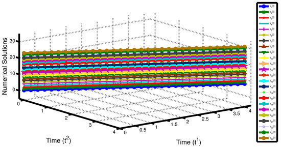
Figure 3. Nguyen traffic network pattern with 24 routes, i.e., $p=24$.

7. Conclusions and Further Developments

This paper is a contribution to the field of noncooperative games. Using a multidimensional approach to time, we have first formulated a multi-time generalized Nash equilibrium problem and a multi-time quasi-variational inequality problem, and then we have established an equivalence between these two problems. Next, we have proved the existence of an equilibrium. As applications of our multi-time generalized Nash equilibrium problem, we have formulated a traffic network model for a courier service company with the aim of minimizing the traffic cost of routes and a river basin pollution problem in the terms of such problems. We have also provided a method for finding equilibria using projected dynamical system theory and have solved the well-known Nguyen traffic network problem by applying our method to it. Indeed, since the decision maker (the company) in this problem aims to minimize the total delivery cost, an optimization reformulation is perhaps more natural than a generalized Nash equilibrium problem (10). Nevertheless, it can be noted that both the feasible traffic flow set and the cost function of each route also depend on the traffic flow of other routes in the generalized Nash equilibrium model (10), but this scenario is not present in an optimization model. In essence, the outcomes of our generalized Nash equilibrium model (10) provide a new approach to solving traffic network problems. We also intend to develop more practical theories and experiments to ascertain that generalized Nash equilibrium models are more efficient than optimization models when applied to traffic network problems. Moreover, we also intend to further explore certain aspects of the river basin pollution problem.

References

- Cournot, A.A. Recherches sur les Principes Mathématiques de la théorie des Richesses; Hachette: Paris, France, 1838. [Google Scholar]
- Nash, J.F. Equilibrium points in n-person games. Proc. Natl. Acad. Sci. USA 1950, 36, 48–49. [Google Scholar] [CrossRef] [PubMed] [Green Version]
- Nash, J.F. Non-cooperative games. Ann. Math. 1951, 54, 286–295. [Google Scholar] [CrossRef]
- Arrow, K.J.; Debreu, G. Existence of an equilibrium for a competitive economy. Econometrica 1954, 22, 265–290. [Google Scholar] [CrossRef]
- Rosen, J.B. Existence and uniqueness of equilibrium points for concave n-person games. Econometrica 1965, 33, 520–534. [Google Scholar] [CrossRef] [Green Version]
- Kesselman, A.; Leonardi, S.; Bonifaci, V. Game-theoretic analysis of internet switching with selfish users. In Internet and Network Economics; Lecture Notes in Computer Science; Deng, X., Ye, Y., Eds.; Springer: Berlin/Heidelberg, Germany, 2005; Volume 3828. [Google Scholar]
- Pang, J.-S.; Scutari, G.; Facchinei, F.; Wang, C. Distributed power allocation with rate constraints in Gaussian parallel interference channels. IEEE Trans. Inf. Theory 2008, 54, 3471–3489. [Google Scholar] [CrossRef]
- Facchinei, F.; Kanzow, C. Generalized Nash equilibrium problems. Ann. Oper. Res. 2010, 175, 177–211. [Google Scholar] [CrossRef]
- Fischer, A.; Herrich, M.; Schönefeld, K. Generalized Nash equilibrium problems-recent advances and challenges. Pesqui. Oper. 2014, 34, 521–558. [Google Scholar] [CrossRef]
- Smith, M.J. The existence, uniqueness and stability of traffic equilibrium. Transp. Res. 1979, 13, 295–304. [Google Scholar] [CrossRef]
- Dafermos, S. Traffic equilibrium and variational inequalities. Transp. Sci. 1980, 14, 42–54. [Google Scholar] [CrossRef] [Green Version]
- Cojocaru, M.G.; Daniele, P.; Nagurney, A. Projected dynamical systems and evolutionary variational inequalities via Hilbert spaces with applications. J. Optim. Theory Appl. 2005, 127, 549–563. [Google Scholar] [CrossRef] [Green Version]
- Nagurney, A. Network Economics: A Variational Inequality Approach; Springer Science and Business Media: Berlin/Heidelberg, Germany, 2013. [Google Scholar]
- Facchinei, F.; Pang, J.S. Finite-Dimensional Variational Inequalities and Complementarity Problems; Springer Science and Business Media: Berlin/Heidelberg, Germany, 2007. [Google Scholar]
- Barbagallo, A.; Cojocaru, M.G. Dynamic equilibrium formulation of the oligopolistic market problem. Math. Comput. Model. 2009, 49, 966–976. [Google Scholar] [CrossRef]
- Cojocaru, M.G.; Bauch, C.T.; Johnston, M.D. Dynamics of vaccination strategies via projected dynamical systems. Bull. Math. Biol. 2007, 69, 453–476. [Google Scholar] [CrossRef]
- Harker, P.T. Generalized Nash games and quasi-variational inequalities. Eur. J. Oper. Res. 1991, 54, 81–94. [Google Scholar] [CrossRef]
- Bensoussan, A. Points de Nash dans le cas de fontionnelles quadratiques et jeux differentiels linéaires a N personnes. SIAM J. Control 1974, 12, 460–499. [Google Scholar] [CrossRef]
- Aussel, D.; Gupta, R.; Mehra, A. Evolutionary variational inequality formulation of the generalized Nash equilibrium problem. J. Optim. Theory Appl. 2016, 169, 74–90. [Google Scholar] [CrossRef]
- Migot, T.; Cojocaru, M.-G. Nonsmooth dynamics of generalized Nash games. J. Nonlinear Var. Anal. 2020, 4, 27–44. [Google Scholar]
- Pang, J.-S.; Fukushima, M. Quasi-variational inequalities, generalized Nash equilibria, and multi-leader-follower games. Comput. Manag. Sci. 2005, 2, 21–56. [Google Scholar] [CrossRef]
- Shehu, Y.; Gibali, A.; Sagratella, S. Inertial projection-type methods for solving quasi-variational inequalities in real Hilbert spaces. J. Optim. Theory Appl. 2020, 184, 877–894. [Google Scholar] [CrossRef]
- Udrişte, C.; Ţevy, I. Multi-time Euler-Lagrange-Hamilton theory. WSEAS Trans. Math. 2007, 6, 701–709. [Google Scholar]
- Udrişte, C. Multitime controllability, observability and bang-bang principle. J. Optim. Theory Appl. 2008, 139, 141–157. [Google Scholar] [CrossRef]
- Udrişte, C. Simplified multitime maximum principle. Balkan J. Geom. Appl. 2009, 14, 102–119. [Google Scholar]
- Udrişte, C.; Dogaru, O.; Ţevy, I. Null Lagrangian forms and Euler-Lagrange PDEs. J. Math. Study 2008, 1, 143–156. [Google Scholar]
- Udrişte, C.; Ferrara, M. Multitime models of optimal growth. WSEAS Trans. Math. 2008, 7, 51–55. [Google Scholar]
- Singh, S.; Pitea, A.; Qin, X. An iterative method and weak sharp solutions for multitime-type variational inequalities. Appl. Anal. 2019. [Google Scholar] [CrossRef]
- Singh, S.; Reich, S. A multidimensional approach to traffic analysis. Pure Appl. Funct. Anal. 2021, 6, 383–397. [Google Scholar]
- Treanţă, S.; Singh, S. Weak sharp solutions associated with a multidimensional variational-type inequality. Positivity 2020. [Google Scholar] [CrossRef]
- Nguyen, S. Estimating Origin Destination Matrices from Observed Flows; Elsevier Science Publishers BV: Amsterdam, The Netherlands, 1984. [Google Scholar]
- Jayswal, A.; Singh, S.; Kurdi, A. Multitime multiobjective variational problems and vector variational-like inequalities. Eur. J. Oper. Res. 2016, 254, 739–745. [Google Scholar] [CrossRef]
- Mititelu, Ş.; Treanţă, S. Efficiency conditions in vector control problems governed by multiple integrals. J. Appl. Math. Comput. 2018, 57, 647–665. [Google Scholar] [CrossRef]
- Ansari, Q.H.; Schaible, S.; Yao, J.C. Generalized vector quasi-variational inequality problems over product sets. J. Glob. Optim. 2005, 32, 437–449. [Google Scholar] [CrossRef]
- Ding, X.P. Existence of solutions for quasi-equilibrium problems in noncompact topological spaces. Comput. Math. Appl. 2000, 39, 13–21. [Google Scholar] [CrossRef] [Green Version]
- Nagurney, A.; Liu, Z.; Cojocaru, M.-G.; Daniele, P. Dynamic electric power supply chains and transportation networks: An evolutionary variational inequality formulation. Transp. Res. E Logist. Transp. Rev. 2007, 43, 624–646. [Google Scholar] [CrossRef]
- Daniele, P. Evolutionary variational inequalities and applications to complex dynamic multi-level models. Transp. Res. E Logist. Transp. Rev. 2010, 46, 855–880. [Google Scholar] [CrossRef]
- Haurie, A.; Krawczyk, J.B. Optimal charges on river effluent from lumped and distributed sources. Environ. Model. Assess. 1997, 2, 177–189. [Google Scholar] [CrossRef]
- Krawczyk, J.B. Coupled constraint Nash equilibria in environmental games. Resour. Energy Econ. 2005, 27, 157–181. [Google Scholar] [CrossRef]
- Krawczyk, J.B.; Uryasev, S. Relaxation algorithms to find Nash equilibria with economic applications. Environ. Model. Assess. 2000, 5, 63–73. [Google Scholar] [CrossRef]
- Kubota, K.; Fukushima, M. Gap function approach to the generalized Nash equilibrium problem. J. Optim. Theory Appl. 2010, 144, 511–531. [Google Scholar] [CrossRef] [Green Version]
- Cojocaru, M.G.; Jonker, L.B. Existence of solutions to projected differential equations in Hilbert spaces. Proc. Am. Math. Soc. 2003, 132, 183–193. [Google Scholar] [CrossRef]
- Cegielski, A. Iterative Methods for Fixed Point Problems in Hilbert Spaces; Springer: Heidelberg, Germany, 2012. [Google Scholar]
- Rockafellar, R.T.; Wets, R.J.-B. Variational Analysis; Springer Science and Business Media: Berlin/Heidelberg, Germany, 2009. [Google Scholar]
Publisher’s Note: MDPI stays neutral with regard to jurisdictional claims in published maps and institutional affiliations. |
© 2021 by the authors. Licensee MDPI, Basel, Switzerland. This article is an open access article distributed under the terms and conditions of the Creative Commons Attribution (CC BY) license (https://creativecommons.org/licenses/by/4.0/).