Zero-Inflated Generalized Linear Mixed Models: A Better Way to Understand Data Relationships

Abstract

Our article explores an underused mathematical analytical methodology in the social sciences. In addition to describing the method and its advantages, we extend a previously reported application of mixed models in a well-known database about corruption in 149 countries. The dataset in the mentioned study included a reasonable amount of zeros (13.19%) in the outcome variable, which is typical of this type of research, as well as quite a bit of social sciences research. In our paper, present detailed guidelines regarding the estimation of models where the data for the outcome variable includes an excess number of zeros, and the dataset has a natural nested structure. We believe our research is not likely to reject the hypothesis favoring the adoption of mixed modeling and the inflation of zeros over the original simpler framework. Instead, our results demonstrate the importance of considering random effects at country levels and the zero-inflated nature of the outcome variable.

1. Introduction

Count data models have increasingly been applied in management research, but the number of studies is still small and further development of this area is needed. As the name suggests, these models have an outcome variable that is a count variable, i.e., a quantitative variable that assumes non-negative and discrete values. Count data models also include several predictor variables, and the statistical objective is to identify and rank the predictor variables that maximize the ability to predict membership in the values of the outcome variable.

The study of Blevins et al. [1] deserves mention since the authors present an in-depth overview of count data models in management. Examples of applications involving count models are the number of times a business firm issues stocks, the number of registered patents over time, and the quantity of branches a company owns/operates. These counts model applications are usually analyzed using generalized linear modeling (GLM), as described by Almeida et al. [2] and O’Hara and Kotze [3], where estimations focus on understanding and explaining how expected counts of membership in the values of the outcome variable change as a function of predictor variables.

In a seminal work, Lambert [4] was bothered by the biases generated by count data models in the presence of a considerable amount of zeros in the outcome variable. Thus, a proposal of a GLM estimation arises that combines a logistic component, in order to identify and better model the excess of zeros (the so-called structural zeros), with a count component which aims to model count data including the remainder of zeros probabilistically considered in the theoretical distributions of this type of estimation (the so-called sample zeros).

This type of GLM is known as a zero-inflated count model. In this type of count model, as already said, the researcher models the outcome variable as a count variable with an excess number of zeros. For instance, when analyzing a firm’s number of patents, one may notice that there are observations when patents were not issued. In such situations, the researcher has two alternatives to obtain model solutions: (1) use methods to deal with the excessive zeros present in the data, or (2) estimate zero-inflated models. Several approaches are available to overcome the first point—excessive zeros in your data (i.e., methods aimed at dealing with outliers). But there are clear alternatives related to the second point—estimating zero-inflated models, since this second approach considers an outcome variable with excess zeros as part of the true data-generating process [5].

However, a limitation of traditional models such as GLM is they don’t allow one to study individual heterogeneities, as well as differences among groups or contexts to which these individuals belong to, or for the specification of random components in different levels (such as groups) of the analysis [6,7]. In other words, traditional GLM methods disregard the natural nesting of the observations, based on the premise that such individuals do not share the same observational context [8], despite the fact that some students can be in the same school or some people share same cultural, social or religious aspects, for instance.

On the other hand, the so-called generalized linear mixed models (GLMM)-also called multilevel models, random coefficients models, nested models, or hierarchical models-act precisely to consider those limitations of the GLM techniques. GLMM estimates, therefore, take into account the existence of dependence among observations from the same group and, consequently, generate unbiased standard errors. Additionally, if the intention is to study if predictor group-level variables interact with individual-level variables, GLMM may be the most adequate estimation [9].

In this sense, the sudy published by Hall [10] deserves mention since it expands Lambert’s [4] ideas to the field of GLMM estimations, considering not only the modeling of the structural and sample zeros, but also the modeling of the count component, taking into account the latent hierarchical groupings evidenced in the dataset.

With this in mind, the objective of this article is to present detailed guidelines regarding the estimation of models where the data for the outcome variable includes an excess number of zeros and the dataset has a natural nested structure. To do so, we use as a starting point one of the well-known models proposed by Fisman and Miguel [11] and compare it with a multilevel zero-inflated negative binomial model (ZINBM) that uses the same variables, but now taking into account the natural nesting of the observations which were originally in their dataset, but were not considered.

This article fills an important gap in methods development since zero-inflated generalized linear mixed models are not yet well explored in management research (according to the best of our knowledge), as discussed in the next sections. We illustrate the main steps related to the estimation of count data, zero-inflated, and zero-inflated multilevel models, and, at the same time, we present estimates of these distinct count models based on a dataset related to corruption practices in a public organization.

The paper is structured as follows: Section 2 discusses zero-inflated and multilevel models, and presents an overview of the articles related to these topics published in the Top 10 journals in the field of strategic management. Section 3 provides an overview on count data models, such as Poisson, negative binomial (NB) with overdispersion concept and zero-inflated. Section 4 presents the generalized linear mixed models (GLMM), with focus on the estimation of the parameters. In Section 5 and Section 6, we offer an illustrative dataset for estimating GLMM through the package glmmTMB available at the Comprehensive R Archive Network (CRAN; http://cran.us.r-project.org (accessed on 28 March 2021)). Section 7 presents our conclusions. Technical details on count data statistical distributions and zero-inflated models, and the R codes, are included in the Appendix A and Appendix B.

2. Background

Zero-inflated regression models are considered a combination of a model for count data with a model for binary data [4]. They are used to identify the reasons why a particular quantity of counts occurs regardless of the number of observed counts. Two types of zero-inflated models are typically estimated, being the first related to the zero-inflated Poisson (ZIP) model estimated from the combination of a Bernoulli distribution with a Poisson distribution, while the second is related to a zero-inflated negative binomial (ZINB) model estimated from the combination of a Bernoulli distribution with a Poisson-Gamma distribution. And one can choose between these two types taking into account existence of overdispersion in the data, i.e., analyzing if the variance of the outcome variable is statistically higher than its mean, as we will discuss in Section 3.

Research in social sciences has dedicated only limited time to the topic of zero-inflated models. A brief review of publications on the topic confirms this point. Table 1 shows the results of searches for terms related to both count models and zero-inflated models in the field of Social Sciences (scholar.google.com.br/ (accessed on 28 March 2021)). Specifically, the table displays each journal’s ranking (column (2)), as well as the number of times the term “Zero-Inflated” is found in a search at each website (column (3)). Table 1 also contains the number of times the terms “Poisson”, “Negative Binomial” and “Overdispersion” appear (columns (4), (5), and (6), respectively). The seventh column combines columns (4) + (5) – (6). Thus, the last column adds the number of times the terms “Poisson” and “Negative Binomial” (two of the most commonly used models in count data analysis) are found, and then subtracts the term “Overdispersion”. The latter term is subtracted to avoid the problem of double counting similar citations, since some of the cited papers may apply both Poisson and NB models when data overdispersion is present. In general, therefore, the seventh column can be considered a proxy for the use of count-based models in social sciences research. The main goal of this search was to obtain initial evidence of the relative importance of zero-inflated models as compared to count-based models.

Table 1. Use of count models and zero-inflated models (ZIM) in the top 10 journals in the field of Social Sciences.

Journal Name (1)	Google Scholar’s Ranking (2)	“Zero -Inflated” (3)	“Poisson” (4)	“Negative Binomial” (5)	“Overdispersion” (6)	Count Models (7) = (4) + (5) − (6)	ZIM Relative Participation (8) = (3)/(7)
Journal of Business Ethics	1	4	36	22	6	52	7.69%
Computers Education	2	2	22	2	0	24	8.33%
American Journal of Public Health	3	32	549	151	85	615	5.20%
Research Policy	4	48	236	248	80	404	11.88%
Global Environmental Change	5	8	36	19	6	49	16.33%
Health Affairs	6	9	76	57	13	120	7.50%
Social Science Medicine	7	36	422	153	60	515	6.99%
New Media Society	8	0	13	15	4	24	0.00%
American Journal of Political Science	9	14	53	54	32	75	18.67%
Procedia-Social and Behavioral Sciences	10	9	100	27	6	121	7.44%

Notes: Authors’ calculations, based on Google Scholar and journals’ data. Search covers all years for all journals. Journals’ ranking positions (column 1) were obtained from Google Scholar for the field of “Social Sciences”. Searches in specific journals were made for the terms “Zero-Inflated” (column 3), “Poisson” (column 4), “Negative Binomial” (column 5), and “Overdispersion” (column 6). Column (7) was obtained by the following column operation: (4) + (5) – (6). The latter column is a proxy for the use of count models in social sciences research top journals. Finally, column (8) was obtained by the column operation: (3)/(7). This column represents the relative participation of zero-inflated models (ZIM) in published articles employing count models. Table completed on 19 March 2021.

When analyzing the results displayed in the last column, one notices that most journals present values in the 5–12% range (the average ratio is 9.00%, while the median is 7.60%). At first, this informal evidence reinforces the notion that zero-inflated models are still underused in contemporary social sciences research, a result in line with previous studies [12].

The results in Table 1 demonstrate that, while there is considerable evidence of count models in social sciences research, there is very limited reporting of zero-inflated journal’s aims and scope, as well as editorial policy, and a more detailed exploration of these empirical patterns appears justified.

It could also be argued that the existence of inflation of zeros in the outcome count variable is a rare event when compared to the non-existence of inflation of zeros. Although the reasoning may make sense for some fields of knowledge, in the field of social sciences, the excess of zeros in the studied phenomenon is not uncommon [13]. Interesting examples of phenomena whose distribution often contains inflation of zeros are traffic accidents [14], insurance claims [15], the arrests unleashed due to the occurrence of human trafficking crimes [16], the behavior of consumption and dependence on alcohol, cigarettes and other drugs by adolescents [17], unemployment issues and their impacts on mental health [18], social, demographic, and economic factors and their impacts on the current Sars-Cov-2 pandemic [19,20]. And the field considered in this paper should also be mentioned, since cultural aspects influencing practices of corruption have not yet been studied from the perspective of the zero-inflated models.

Blevins et al. [1] previously presented a detailed exposition of count models specifically in management research. The authors started their analysis by reviewing 11 years of management research using count-based outcome variables in 10 leading journals. They found that, while one of four papers in their sample used the basic Poisson regression model to estimate count outcome variables, alternative models might have been more appropriate in such occasions.

In fact, in many of the applications considered by the authors, we believe an alternative zero-inflated model might have provided a better fit for the data. In drawing this conclusion, the authors compared different count models estimated with previously published data and, at the same time, ran simulations based on different parameter values. The results also concluded that, in some cases, there was the possibility of significance level changes in some regressors, as well as sign changes.

In addition, we argue that the consideration of the natural nesting of the observations should also be taken into account in conjunction with the inflation of zeros for the count data models. This is an important qualification since GLM do not take into account a possible grouping of observations within a nested data structure. However, household residences belonging to the same neighborhood, or different students from the same school are often correlated, and these correlations can be accounted for in GLMM with the consideration of random effects [21,22] (As the authors note: “Despite the benefits of using these models, the use of zero-inflated models is only recently gaining traction in management research. Our review showed that only a small percentage of management scholars (11%) used such models” [1]. We view the results presented in Table 1 as robust evidence to these authors’ claims.).

In short, in comparison with the classic GLM, GLMM estimations have the advantage of proposing a structure with different levels, and each of these levels is investigated by its own model. According to Woltman et al. [23], each level tries to capture the behavior of the variables and specifies how these variables are related to and influence other levels. As discussed by Courgeau [8], GLMM enables the researcher to relate observations and contexts, such as firms and countries, students and schools, or families and neighborhoods. If one decides to ignore these relationships, incorrect interpretations can arise.

The mixed designation in the GLMM term comes from the fact that predictor variables can be considered in both fixed and random effects components of the regression model. The estimated parameters of fixed effects indicate the relationship between predictor variables and the outcome variable (as well as in the context of GLM estimations), while the random effects component can be represented by the combination of error terms and predictor variables. Recent contributions on the benefits of mixed models are found in References [24,25,26,27,28,29,30,31]. All of these studies emphasized that multilevel models are a generalization of regression methods and, thus, can be applied for prediction and also for causal inference based on observational studies.

Mixed models, a term that also commonly appears in the literature as multilevel models, hierarchical models or random coefficients models have acquired considerable importance in the social sciences, and the publication of papers that consider these estimations have been increasingly more frequent, mainly due to studies that take into account the existence of nested data structures. Table 2 displays the search results for the terms “Multilevel Model”, “Hierarchical Model”, and “Random Coefficients Model” in Social Sciences (scholar.google.com.br/(accessed on 28 March 2021)). While the analysis shows a meaningful number of papers in top social sciences research journals that apply some type of mixed modeling, our research was unable to find in these same journals a single paper with zero-inflated estimations and, simultaneously, with a multilevel perspective, i.e., that takes into account the existence of a nested data structure.

Table 2. Use of GLMM in the top 10 journals in the field of Social Sciences.

Journal Name (1)	Google Scholar Ranking (2)	“Multilevel Model” (3)	“Hierarchical Model” (4)	“Random Coefficients Model” (5)	GLMM (6) = (3) + (4) + (5)
Journal of Business Ethics	1	60	47	13	120
Computers & Education	2	62	27	0	88
American Journal of Public Health	3	59	20	2	81
Research Policy	4	35	22	6	63
Global Environmental Change	5	25	13	1	39
Health Affairs	6	2	7	0	9
Social Science Medicine	7	727	149	36	912
New Media Society	8	2	7	0	9
American Journal of Political Science	9	38	17	1	56
Procedia-Social and Behavioral Sciences	10	72	144	6	22

Notes: Authors’ calculations, based on Google Scholar and journals’ data. Search covers all years for all journals. Journals’ ranking positions (column 1) were obtained from Google Scholar for the field of “Social Sciences”. Searches in specific journals were made for the terms “Multilevel Model” (column 3), “Hierarchical Model” (column 4), and “Random Coefficients Model” (column 5). Column (6) brings the sum of columns (3), (4) and (5), i.e., represents a proxy for the total amount of papers that make use of mixed models in social sciences research top journals. Table completed on 19 March 2021.

In addition to what is shown in Table 1 and Table 2, studies that estimate models taking into account, simultaneously, the inflation of zeros in the outcome variable and the multilevel structure of the dataset are quite rare. Based on our search, zero-inflated generalized linear mixed models are not yet very widely explored in social sciences.

3. Count Data and Zero-Inflated Models

Understanding the probability distributions and algebraic and econometric criteria for estimating parameters is crucial for the definition of predictive equations that try to capture, in a more reliable way, the real behavior of data.

Nelder and Wedderburn [32], in a relevant paper, presented and discussed through theoretical and conceptual points of view, several works that had previously estimated logistic models involving Bernoulli and binomial distributions, count data models involving Poisson distribution, and polynomial models involving Gamma distribution, among others. All these model estimations were combined in a group referred to as GLM [29]. As part of GLM discussions, therefore, count data regression models can be estimated for cases in which the the otcome variable is quantitative with discrete and non-negative values. Moreover, both Cameron and Trivedi [33] and Hilbe [34,35] note that these estimations are more adequate that traditional linear regression models, which can fail to take into account the presence of discrete and non-negative values in the outcome variables.

Wooldridge [36] indicates that a general regression model for count data can be described using Expression (1) as follows:

$${\widehat{Y}}_i={\lambda }_i=exp({\beta }_0+{\beta }_1{X}_{1i}+{\beta }_2{X}_{2i}+...+{\beta }_k{X}_{ki}),$$

(1)

where ${\lambda }_i=exp({\beta }_0+{\beta }_1{X}_{1i}+{\beta }_2{X}_{2i}+...++{\beta }_k{X}_{ki})$ represents the expected number of occurrences or incidence rate ratio of the phenomenon studied for a given exposure; ${\beta }_0$ is the intercept; ${\beta }_j(j=1,2,3,...,k)$ are the coefficients estimated for each predictor variable $X_i$; k is the number of predictor variables used in the model; and i indicates each observation of a given sample.

While Poisson models assume the existence of equidispersion of the count data for the variable of interest, i.e., ${\mu }_i=E\left(Y_i\right)=Var\left(Y_i\right)={\lambda }_i$, the estimation of a NB model assumes overdispersion of the outcome variable, conditional to predictor variables Hilbe [35], i.e., ${\mu }_i=E\left(Y_i\right)<Var\left(Y_i\right)={\lambda }_i$. Expressions (2) and (3) represent the mean and the variance, respectively, for a negative binomial model.

$$E\left(Y_i\right)=u_i,$$

(2)

$$Var\left(Y_i\right)=u_i+\varphi u_i^2,$$

(3)

where $\varphi =\frac{1}{\psi }$ and $u_i=exp({\beta }_0+{\beta }_1{X}_{1i}+{\beta }_2{X}_{2i}+...++{\beta }_k{X}_{ki})$.

As discussed by Cameron and Trivedi [37], the parameter $\varphi$ in expression (3) represents overdispersion in the count data. According to Fávero et al. [38], in the cases where $\varphi \to 0$, equidispersion would be detected in the dataset used, indicating that a Poisson regression model should be used. In addition, according to the authors, for the case in which $\varphi$ is statistically greater than zero, the phenomenon of overdispersion would occur, which suggests the use of the NB model.

Although the most commonly used model for the analysis of count data is the Poisson model, by definition, its distribution has a single free parameter, $\lambda$, thus not allowing the variance to be fitted to the mean [33,39], as previously explained for the case of $\lambda =Var\left(Y\right)$. Thus, in the presence of overdispersion, a NB model can provide a better fit for the count data, in which the mean of the Poisson distribution can be used as a random variable that follows a Gamma distribution, together with an additional free parameter $\varphi$ [40].

Additionally, it is common that some count data variables show a great amount of values equal to zero, which represents a fact that can generate biases in the parameters estimated through traditional Poisson or NB regression models, since these models do not take into account the heightened presence of zero counts. In these cases, the consideration of zero-inflated regression models makes sense [5].

In this perspective, according to Lambert [4], zero-inflated regression models are used for investigating the reasons why a certain number of counts occur, including zeros, and the reasons why this quantity happens, regardless of the number of observed counts. As stated in Ngatchou-Wandji and Paris [41], zero-inflated regression models can be defined as follows:

$$p(Y=y|\omega )=\omega {\delta }_0\left(y\right)+(1-\omega )f\left(y\right),$$

(4)

where Y is the count variable, $\omega$ is the proportion of the excess of zeros, ${\delta }_0\left(y\right)=1$ if $y=0$ and ${\delta }_0\left(y\right)=0$, otherwise; and f$\left(y\right)$ is the density of a count distribution, such as Poisson or NB.

In this sense, ZIP models can be estimated through the consideration, simultaneously, of Bernoulli and Poisson distributions. On the other hand, ZINB models are estimated through the simultaneous consideration of Bernoulli and Poisson-Gamma distributions. And one can choose the best estimation depending on the existence of overdispersion in the data [13]. In other words, this decision can be made taking into account the statistical significance of the inverse of the Gamma distribution parameter. And the definition of the existence or not of an excessive amount of zeros in the outcome variable is determined through the analysis of the outputs of the Vuong Test [42]. Table 3 shows the relationship between count data models, overdispersion, and inflation of zeros.

Table 3. Count data regression models, overdispersion, and inflation of zeros in the outcome variable.

Verification	Count Data Regression Model
	Poisson	Negative Binomial (NB)	Zero-Inflated Poisson (ZIP)	Zero-Inflated Negative Binomial (ZINB)
Overdispersion in Outcome Variable	No	Yes	No	Yes
Inflation of Zeros in Outcome Variable	No	No	Yes	Yes

Notes: Extracted from Fávero and Belfiore [29].

According to Table 3, while ZIP and ZINB regression models are more appropriate in the presence of an excessive amount of zeros in the outcome variable, the use of the latter is further recommended if there is overdispersion in the data. Technical details on statistical distributions, as well as on count data and zero-inflated regression models, are included in Appendix A and in the supplementary material.

4. Generalized Linear Mixed Models (GLMM)

Multilevel models have become quite important in several fields of knowledge, including management. The main reason is that some research constructs are taking into account the existence of nested, or mixed, data structures, in which certain variables vary among groups, or contexts, but do not vary among observations from the same context [21,43]. In addition, computational developments that have increased processing capacities allow the estimation, increasingly, of different types of multilevel models [29,44,45].

4.1. The Two-Level Model

According to Fávero [46], there are many situations where data are disposed within a mixed, or nested structure, and the hierarchies refer to fact that observations from the same groups, or contexts, share aspects, or characteristics, that represent a kind of homogeneity.

In this perspective, a two-level zero-inflated count data mixed model, in this sense, can be specified, where the first level refers to observations $i(i=1,...,n)$, nested in two-level units $j(j=1,...,J)$, as follows:

$$ln\left(\frac{p_{logi{t}_{ij}}}{1-p_{logi{t}_{ij}}}\right)={\mathbf{Z}}_{ij}^T\delta , \mathrm{being} \delta ={\mathbf{G}}_j^T\alpha ,$$

(5)

$$ln\left({\lambda }_{ij}\right)={\mathbf{X}}_{ij}^T\pi +{\nu }_j, \mathrm{being} ={\mathbf{H}}_j^T\beta ,$$

(6)

where matrices of the predictor variables $\mathbf{Z}$ and $\mathbf{X}$, of levels i (level 1) and j (level 2), appearing in the respective logistic (Bernoulli) and Poisson or Poisson-Gamma components are not necessarily the same (equal conditions hold for matrices of the variables ${\mathbf{G}}_j$ and ${\mathbf{H}}_j$ at level two), and $\mathit{\delta }$, $\mathit{\pi }$, $\mathit{\alpha }$, and $\mathit{\beta }$ are the respective matrices of the regression parameters, i.e., $\mathit{\delta }$ can be interpreted in terms of the proportion of inflation of zeros, $\mathit{\pi }$ is related to the mean response in the count data part, and $\mathit{\alpha }$ and $\mathit{\beta }$ correspond to differences among level two context in structural and sample zeros, respectively, due to the behavior of predictor variables in level two (${\mathbf{G}}_j$ and ${\mathbf{H}}_j$). Following Lee et al. [47] and Fávero et al. [40], ${\mathit{\delta }}_j$ represents the random variations at second level, which means that heterogeneity among higher levels of analysis (groups, for instance) and between individuals is allowed through the random effects $\mathit{\delta }$, with variance equal to ${\mathit{\sigma }}^2{\mathit{\nu }}_j$.

Despite the fact that Rabe-Hesketh et al. [48] discuss and estimate multilevel models taking into account discrete outcome variables, papers that consider zero-inflated count data regression models with random effects in the literature are still quite limited.

4.2. Model Estimation and Materials

As discussed by Lee et al. [47], one can estimate zero-inflated generalized linear mixed models considering the restricted maximum likelihood approach. The definition the GLMM likelihood function requires the specification of the log-likelihood function of the fixed component (first term), as well as the logarithm of the probability density function of the random effects (second term), which allows one to specify more complex correlation structures in the variance components.

Lee et al. [47] present the log-likelihood function for zero-inflated count data mixed models. The first term, $L{L}_1$, is given by Expressions (A14) or (A19) presented in Appendix A and is related to ZIP and ZINB estimations, respectively, depending on the existence of overdispersion on data. The second term is given by:

$$L{L}_2=-\frac{1}{2}[nln\left(2\mathit{\pi }{\mathit{\sigma }}_{\nu }^2\right)+{\mathit{\sigma }}_{\nu }^{-2}{\mathit{\nu }}^T\mathit{\nu }].$$

(7)

Random effects $\mathit{\nu }$ allow the existence of heterogeneity among clusters and also among individuals. Estimation proceeds by maximizing $L{L}_1$ (A14) or (A19) with the consequent update of the values of the variance components through the estimation of a restricted maximum likelihood (REML) function from LL2 [46]. Thus, $L{L}_1+L{L}_2$ generates the final $LL$ for a zero-inflated multilevel model. In the next section, we will estimate and present the parameters of one of the original models proposed by Fisman and Miguel [11], the NB estimation, which the authors called Model 3, including its analogous model that considers the inflation of zeros (ZINB estimation), as well as the model that considers the inflation of zeros under the multilevel perspective (ZINBM estimation).

With that said, first, one can study the statistical significance of the excessive amount of zeros in the outcome variable Y through the application of the Vuong test. Subsequently, the study can be conducted taking into account an eventual hierarchical structure of the observations in the dataset of Fisman and Miguel [11].

Finally, the log-likelihood values of the estimated models were compared to enable one to verify the best suitability for the considered data, and pointing out the biases generated by not considering the inflation of zeros and/or the nested structure of the data.

In this paper, all the estimations are obtained through the software R version 4.0.4, using the package MASS for the NB models, the package pscl for the ZINB model, and the package glmmTMB for the ZINBM model.

5. Culture and Corruption among United Nations’ Diplomats: An Applied Example

Corruption is an important matter. For instance, when analyzing the effect of corrupt practices on economic outcomes for a cross-section of countries, Mauro [49] finds that corruption lowers private investment and long-run growth. In fact, there is an ever-growing literature aimed at studying and measuring corruption, both in individual and aggregate levels [50,51,52].

In this section, we present an application related to zero-inflated generalized linear mixed models for the study of corruption practices in organizations. We used the paper’s code in Stata and respective datasets available at Edward Miguel’s website, despite the fact that Fisman and Miguel also made available other versions. We first made extensive use of the materials available there, such as the authors’ data codebook, for instance (The original datasets and code are available at the following links: https://dataverse.harvard.edu/dataset.xhtml?persistentId=doi:10.7910/DVN/28059 (accessed on 28 March 2021) and http://emiguel.econ.berkeley.edu/research/corruption-norms-and-legal-enforcement-evidence-from-diplomatic-parking-tickets (accessed on 28 March 2021). As an additional note, we did not get in touch with the authors in order to use their public dataset.).

Fisman and Miguel [11] presented an original approach to study corruption in a sample of countries. The authors explore based on a unique point of view: the parking behavior of United Nations’ (UN) diplomats. They analyzed parking violations from worldwide diplomats during the 1997–2005 period. Given that, since in part of the considered period diplomatic immunity protects UN diplomats from parking enforcement actions, while in the subsequent period diplomatic immunity for parking enforcement actions no longer occurs, the authors argue that diplomats’ behavior regarding parking tickets can be considered a good proxy for cultural aspects which can determine corrupt behavior.

Based on this data, the authors built a “revealed preference” measure of corruption among officials who work for governments of 149 countries. This measure has the advantage of being based on diplomats’ observed actions, which is its main feature, given the well documented difficulties in measuring corruption worldwide [53] (The authors also built a ranking of countries based on parking violations. In the first positions of the ranking come Kuwait, Egypt and Chad (as more corrupt countries), while Japan, Norway, and Sweden are among the least corrupt in the sample [11].).

Fisman and Miguel [11] bring an interesting discussion emphasizing that parking violation corruption is strongly (and positively) correlated with some country corruption measures, such as those defined by the World Bank surveys, for instance. In general terms, this result suggests that home country corruption norms may serve as a predictor for the propensity to behave corruptly among government officials. Specifically, the data reveals that diplomats from high-corruption countries (such as Nigeria, for instance), on average, tend to behave remarkably bad in situations in which there are no legal consequences involved, while the opposite is true for diplomats from low-corruption countries (such as Norway), whose diplomats do not tend to commit more parking violations.

We begin by replicating a graphical pattern contained in the data. Figure 1 shows the scatterplot relating unpaid parking violations (vertical axis, in natural logarithmic scale) and country corruption measures (horizontal axis), considering the period of non-existence, as well as the period of existence of legal consequences for unpaid parking violations by diplomats (in Figure 1, the label ’no’ means no legal consequences, while the label ’yes’ means the opposite). The plot suggests a positive (and possibly nonlinear) relationship between diplomats’ traffic violations and each country’s corruption measures.

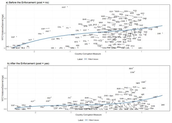
Figure 1. Parking violations and country corruption index from Fisman and Miguel [11] dataset.

As a second step, Figure 2 presents a histogram containing unpaid diplomats’ parking violations, i.e., the outcome variable on Fisman and Miguel’s Model 3, called by the authors violations_all. We construct this figure to provide a visual representation of zero values contained in the outcome variable, as well as to emphasize the likely overdispersion present in the outcome variable.

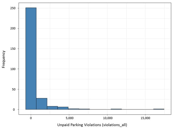
Figure 2. Histogram of the outcome variable (violations_all).

The graphical patterns described in Figure 2 shows the occurrence of zero values in 13.19% of the sample containing the outcome variable. At first, there is still no way to affirm the need of estimation of zero-inflated models based only on Figure 2, and more formal tests are needed before reaching stronger conclusions. Table 4 presents the variables used in Fisman and Miguel’s Model 3, which were considered in the replication model under the multilevel perspective with inflation of zeros. For more information on the variables, see Fisman and Miguel [11].

Table 4. Description of the variables considered in the Fisman and Miguel’s Model 3.

Variable	Description
wbcode	Polychotomic categorical variable that indicates the acronyms of the countries in the dataset.
region	Polychotomic variable that points to a region of the globe to which each country in the dataset belongs: Africa, Asia, Europe, Middle East, North America, Oceania, and South America.
violations_all	Discrete variable that measures the amount of unpaid parking violations by diplomats in a givencountry. It is the outcome variable of the models.
corruption	Continuous variable that indicates the level of corruption in each country. The greater the polarity, the greater the country’s corruption.
post	Dichotomous variable that indicates the moments that consider the inexistence and existence of legal consequences to unpaid parking violations by diplomats-’no’ and ’yes’ indicators, respectively.
staff	Discrete variable that measures the number of diplomats from a given country.
lgdppcus	Continuous variable that indicates the natural logarithm of GDP per capita of each country.

Table 5 presents the descriptive statistics of the quantitative variables, as well as the frequency tables of the qualitative variables explained in Table 4, which, in fact, were considered in the so-called Model 3 proposed by Fisman and Miguel [11].

Table 5. Univariate descriptive statistics of the quantitative variables and frequency table of the qualitative variables that were considered in the models.

Violation_all	Corruption	Post	Staff	Lgdppcus	Region
Min.: 0.0 1st Q.: 2.0 Median: 18.5 3rd Q.: 253.8 Max: 16,751.0 Mean: 494.6	Min.: −2.583 1st Q.: −0.415 Median: 0.327 3rd Q.: 0.720 Max: 1.583 Mean: 0.014	Freq. of ‘no’: 149 Freq. of ‘yes’: 149	Min.: 2.000 1st Q.: 6.000 Median: 9.000 3rd Q.: 14.000 Max: 86.000 Mean: 11.810	Min.: 4.559 1st Q.: 6.036 Median: 7.266 3rd Q.: 8.543 Max: 10.505 Mean: 7.394	Africa: 92 Asia: 50 Europe: 70 Middle East: 30 North America: 12 Oceania: 8 South America: 36

Note 1: Q. stands for quartile. Note 2: Freq. stands for Frequency. Note 3: North America data includes Caribbean data.

In terms of econometric methodology, Fisman and Miguel (2007) estimated a count data NB regression model. In Table 6, in addition to the original NB model proposed by Fisman and Miguel [11], we present a ZINB estimation (necessary for the application of the Vuong test), and a ZINBM estimation using exactly the same variables as the initial NB model.

Table 6. Estimations of negative binomial model [11], and correspondent zero-inflated and zero-inflated mixed model.

	NB–Model 3 Fisman and Miguel [11]	ZINB	ZINBM
Fixed Effects
intercept	2.871 ***	3.115 ***	2.732 **
	(0.987)	(0.909)	−1,150
corruption	0.575 ***	0.475 ***	0.561 ***
	(0.162)	(0.159)	(0.215)
post	−4.215 ***	−4.284 ***	−4.265 ***
	(0.175)	0.153	(0.136)
staff	0.051 ***	0.048 ***	0.040 ***
	(0.008)	(0.011)	(0.011)
lgdppcus	0.091	0.110	0.105
	(0.116)	(0.112)	(0.129)
Africa	2.865 ***	2.657 ***	2.885 ***
	(0.504)	(0.466)	(0.642)
Asia	1.985 ***	1.771 ***	2.133 ***
	(0.518)	(0.484)	(0.668)
Europe	2.237 ***	1.991 ***	2.020 ***
	(0.510)	(0.500)	(0.656)
Middle East	3.229 ***	3.084 ***	3.045 ***
	(0.544)	(0.533)	(0.707)
Oceania	1.508 **	1.399 **	1.832 **
	(0.739)	(0.679)	(0.922)
South America	1.667 ***	1.453 ***	1.671 **
	(0.533)	(0.515)	(0.684)
Logistic Component
intercept	-	−2.432 ***	−2.331 ***
		(0.298)	(0.260)
corruption	-	−0.695 ***	−0.564 ***
		(0.204)	(0.212)
Random Effects
$Var\left({\nu }_{0j}\right)$-intercept	-	-	0.502
$Var\left({\nu }_{1j}\right)$-slope (corruption)	-	-	0.296
Observations	298	298	298
Log-likelihood ($LL$)	−1547.691 (df = 12)	−1526.838 (df = 14)	−1515.049 (df = 17)

Note: Standard errors are in parentheses. The omitted region category is North America/Caribbean. ** Statistically significantly different from zero at 95 percent confidence. *** Statistically significantly different from zero at 99 percent confidence.

6. Results and Discussions

The confirmation of overdispersion of the outcome variable, conditional to predictor variables, comes from the Cameron and Trivedi test [37], whose result is in Figure 3. In Appendix A, we present further details on the diagnosis of overdispersion.

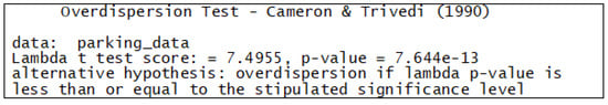
Figure 3. Result of the Cameron and Trivedi overdispersion test.

The verification of the existence of excess of zeros in the outcome variable unpaid parking violations (violations_all) can be elaborated in sequence, through the Vuong test, which compares likelihood functions between a GLM estimation, such as the NB, with the respective estimation with eventually an inflation of zeros. Table 7 shows the results for the Vuong test when comparing the NB regression model with the corresponding ZINB model.

Table 7. Results of the Vuong test-ZI negative binomial x negative binomial.

	Vuong z-Statistic	p-Value
Raw	2.953160	0.0015727
AIC-corrected	2.669934	0.0037933
BIC-corrected	2.146377	0.0159215

Notes: Vuong non-nested hypothesis test-statistic: test-statistic is asymptotically distributed N (0,1) under the null hypothesis that the models are indistinguishable.

Since the Vuong test might be biased towards supporting models with zero-inflation components, according to Desmarais and Harden [54], we implemented Desmarais and Harden’s correction to verify if the former results are somehow affected. While the Vuong test statistic is $z=2.95$, the AIC and BIC corrected statistics are $z=2.67$ and $z=2.15$, respectively, or rather, all present p-values $<0.05$. These results indicate the better adequacy of the zero-inflated negative binomial regression model, in comparison with the traditional GLM negative binomial regression model estimated by Fisman and Miguel [11].

Such a diagnosis, which points out the better suitability of the ZINB estimation, by itself, would already suggest that the original NB estimation present biases by not considering the excess of zeros in the outcome variable. Furthermore, the NB estimation fails to identify that the slope of the variable corruption, in the ZINB logistic component, indicates that an increase in one unit leads to a 50.01% decrease, on average, in the chance of structural zeros, ceteris paribus, since $exp(-0.695)=0.499$. In other words, the variable corruption has an even greater preponderance in the absence of unpaid parking violations by diplomats in the considered countries.

This fact leads to a second important bias: the NB model overestimates almost all parameters of the other variables that were shown to be statistically significant, when compared to the count component of the ZINB estimation, although there is no inversion of signs-the exception occurs for the variable post.

When the original NB model is compared to the ZINBM estimation, which takes into account the nested structure of data among countries, the biases are more striking. The first point to note is that the consideration of these groupings leads to a smoothing of the slope of the variable corruption in the logistic component in comparison with the ZINB model.

The value of the slope parameter of the ZINB logistic component is $-0.695$; for the ZINBM estimation, $-0.564$. In other words, when considering the nested structure among countries, the chance of existence of structural zeros in the dataset is reduced, on average, by 43.10% when increasing the variable corruption in one unit, ceteris paribus, since $exp(-0.564)=0.569$. It is also interesting to note that the NB model cannot even capture the ratio of the inflation of zeros in the dataset and, even if the ZINB model succeeds, it reasonably overestimates the studied situation by neglecting the natural nesting in the data.

When considering the existing nested structure in the dataset of Fisman and Miguel [11], we realize that there is an overestimation of the parameters of the NB model, regarding both the general intercept and the slopes of the predictor variables corruption, staff, Europe, and Middle East, when compared to the ZINBM model. On the other hand, the NB estimation underestimates the parameters of the other variables when compared to the ZINBM estimation. There was also no inversion of signals.

Thus, in the NB model, the dummy variable that identifies the Oceania region has a coefficient equal to 1.508, against 1.832 for the ZINBM model. Thus, when adopting the North America region as the reference region, the NB model predicts, on average, an increase in the chance of occurrence of the outcome variable in 351.77%, if the diplomat is from Oceania, keeping the other conditions constant. The ZINBM model, on the other hand, intensifies this situation, since the increase in the chance of occurrence of the outcome variable, on average, is 524.64% if the diplomat is from Oceania, taking the region North America as a reference, ceteris paribus. In short, the NB model underestimates the occurrence of unpaid parking violations among diplomats from Oceania region by 67.05% when compared to the ZINBM estimation. Using this same approach, when compared to the ZINBM estimation, the NB model underestimates the impact of the Asia region by 15.95%.

The parameter related to the Europe region also draws attention. The NB model overestimates the chance of unpaid parking violations among diplomats, on average, by 27.94%, ceteris paribus, when compared to the ZINBM model and being North America as the reference region. Under the same perspective, for the Middle East region, the NB estimate overestimates the impact by 20.20%.

Behind a functional form that is better adherent to the data of Fisman and Miguel [11], the ZINBM estimation has the ability to estimate random effects for the groups that characterizes the hierarchical levels—countries, in this case. Thus, the proposed model presents different error terms related to intercepts and slopes for each country.

Equation (8) presents the NB model proposed by Fisman and Miguel [11]; Equation (9) brings the result of the ZINB estimation, showing both the logistic and the count components; finally, Equation (10) demonstrates the ZINBM estimation, its logistic and count components, and the random error terms for the intercepts (${\nu }_{0j}$) and for the slopes due to the corruption variable (${\nu }_{1j}$). Random effects (${\nu }_{0j}$) and (${\nu }_{1j}$) of the ZINBM estimation are presented in Appendix B.

$$\begin{array}{cc}{\widehat{violations\_all}}_{N{B}_i}& =2.871+0.575.corruptio{n}_i-4.215.pos{t}_i+0.051.staf{f}_i+\hfill \\ & 0.091.lgdppcu{s}_i+2.865.Afric{a}_i+1.985.Asi{a}_i+2.237.Europ{e}_i+3.229.MiddleEas{t}_i+\\ & \hfill 1.508.Oceani{a}_i+1.667.SouthAmeric{a}_i,\end{array}$$

(8)

$$\begin{array}{cc}{\widehat{violations\_all}}_{ZIN{B}_i}& =\left\{1-\frac{1}{1+exp[-(-2.432-0.695.corruptio{n}_i)]}\right\}.exp[3.115+\hfill \\ & 0.475.corruptio{n}_i-4.284.pos{t}_i+0.048.staf{f}_i+0.110.lgdppcu{s}_i+2.657.Afric{a}_i+\hfill \\ & \hfill 1.771.Asi{a}_i+1.991.Europ{e}_i+3.084.MiddleEas{t}_i+1.399.Oceani{a}_i+1.453.SouthAmeric{a}_i],\end{array}$$

(9)

$$\begin{array}{cc}{\widehat{violations\_all}}_{ZINB{M}_{ij}}& =\left\{1-\frac{1}{1+exp[-(-2.3313-0.5643.corruptio{n}_{ij})]}\right\}.exp[2.732+\hfill \\ & 0.561.corruptio{n}_{ij}-4.265.pos{t}_{ij}+0.040.staf{f}_{ij}+0.105.lgdppcu{s}_{ij}+2.885.Afric{a}_{ij}+\\ & 2.133.Asi{a}_{ij}+2.020.Europ{e}_{ij}+3.045.MiddleEas{t}_{ij}+1.832.Oceani{a}_{ij}+\\ & \hfill 1.671.SouthAmeric{a}_{ij}+{\nu }_{0j}+{\nu }_{1j}.corruptio{n}_{ij}].\end{array}$$

(10)

Looking again at Table 6, it is interesting to note that the increase in $LL$ between the models could be said to be modest, but in all cases, according to a likelihood ratio test, it is statistically significant at 1%. More than that, when analyzing, for example, the fitted values of the ZINBM model considering the predictor variable staff, which has not yet been explored, it is difficult to advocate in favor of the NB model, as shown in Figure 4.

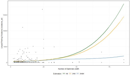
Figure 4. Fitted values of NB, ZINB, and ZINBM estimations, considering the predictor variable staff.

According to Figure 4, it is evident that the NB estimation is unable to adequately capture the inflation of zeros present in the dataset. It is also interesting to note that, for the ZINB estimation, even though it captures the excess of zeros better than the NB model, there is no ability to adequately segregate, due to natural nesting (countries), the occurrence of structural zeros. In fact, the ZINBM estimation is superior to all others for the case studied.

7. Final Considerations

After exploring different approaches to a well-known NB model, we propose to divide our final considerations into three main parts: theoretical aspects, managerial implications and future research in count data multilevel modeling.

7.1. Theoretical Aspects

In this article, we presented guidelines for the estimation of zero-inflated generalized linear mixed models. That is, models where the outcome variable presents an excess number of zeros and the dataset has a structure where observations are correlated in ways that require random effects.

As an illustration of the importance of zero-inflated generalized linear mixed models, we presented an application based on a dataset related to corruption practices among UN’s diplomats [11]. We emphasize that, in no way, we tried to diminish the merit of the study and the authors’ findings. Furthermore, at the time of the study, multilevel models were rare and computational capabilities represented a considerable constraint. Our main message is about the superiority of GLMM models, in relation to GLM, when the natural nesting of observations is available to researchers.

We were able to replicate the original study’s main results, confirming their authors’ claims regarding the role of cultural norms for corrupt behavior. We found a strong effect of corruption norms: diplomats from high-corruption countries (on the basis of existing survey-based indices) accumulated significantly more unpaid parking violations, i.e., cultural norms can be seen particularly as an important determinant of corruption (Table 6 and Equations (8)–(10)).

We also extended their original analysis by estimating zero-inflated generalized linear mixed models. At one hand, the reported results confirm Fisman and Miguel’s original findings, in terms of estimated signs and statistical significance (Table 6). On the other hand, the results allow us to discuss the importance of considering different zero-generating processes for outcome variables, also taking into account the nature and the structure of the considered dataset. In this sense, we are cannot reject the hypothesis favoring the use of ZINBM model over the traditional GLM models.

7.2. Managerial Implications

Management research still uses count-based models with parsimony [1,12]. Although there has been an increase in the use of such models, there is still considerable room for improvement, given the many opportunities related to interesting themes, such as patents, product innovations, and issue of shares, for instance. In fact, even when studying the influence of social factors over behavior, such as social ties, researchers might benefit from using count models [13].

While we believe the results presented here provide additional evidence supporting the use of count-based models, we emphasize the importance of zero-inflated generalized linear mixed models for specific applications. In a broader sense, these results are important for emphasizing potential uses of this class of models in distinct areas of management research. We agree with Blevins et al. [1], who discuss that there is still room for improvement in terms of existing research practices. Specifically, both researchers and practitioners could obtain substantial gains and insight by incorporating in their toolkit’s models with excess zeros in the outcome variable in a multilevel perspective.

By presenting this guideline and applied example related to zero-inflated linear mixed models, we hope to see more studies of this kind in the near future, as well as to stimulate the development of new ways to analyze and interpret quantitative data in management research, as originally proposed by other authors [55,56]. By the way, Dale and Sirchencko [57] bring an important example in this regard.

In addition, we believe that datasets from organizational research sometimes do not explicitly represent contexts that can be defined as levels of analysis in multilevel modeling. Regardless, researchers and practitioners can create clusters from the observations’ own data, allowing the establishment of latent higher-level random effects (in this case, at the level of the cluster itself), even if there are no variables corresponding to these clusters. Due to the fact that cluster analysis is an unsupervised exploratory technique, the predictive power of the estimation will be lost, but even so the model can be more adequately adjusted for diagnostic purposes regarding the behavior of the existing data.

7.3. Future Research in Count Data Multilevel Modeling

In our research, we did not find studies that estimate zero-inflated multilevel models using longitudinal data, in which the temporal dimension represents level 1 of the analysis. This can be an interesting prospect for future research.

Another relevant point is that we did not discuss endogeneity problems arising from the fact that entities such as individuals, organizations or countries can vary systematically from one another. As discussed by Antonakis et al. [58], researchers typically estimate multilevel models assuming the random effects are uncorrelated with the regressors. But this problem can be avoided by including cluster means of level 1 explanatory variables as controls.

From our research search, we did not find works that discuss these points and problems in estimations of Count Data Multilevel Models with inflation of zeros.   

Appendix A.1. Poisson Regression Models

According to Cameron and Trivedi [33], in general Poisson regression models can be applied when the distribution of the occurrence of a given phenomenon being studied follows a Poisson distribution, as shown in Figure A1, where p represents, for a determined observation $i(i=1,2,\dots ,n)$, the probability of occurrence of a specific count for a determined exposition m (such as geographic region or period of time, for instance), as shown in Expression (A1).

Figure A1. The Poisson distribution.

$$p(Y_i=m)=\frac{exp(-{\lambda }_i).{\lambda }_i^m}{m!}, \mathrm{being} m=0,1,2,...$$

(A1)

Klakattawi et al. [59] argue that Poisson models assume the existence of equidispersion of the count data for the variable of interest; i.e., ${\mu }_i=E\left(Y_i\right)=Var\left(Y_i\right)={\lambda }_i$, in accordance with Expressions (A2) and (A3), as follows:

$$E\left(Y_i\right)=\sum _{m=0}^{\infty }m\frac{exp(-{\lambda }_i).{\lambda }_i^m}{m!}=\lambda \sum _{m=1}^{\infty }\frac{exp(-{\lambda }_i).{\lambda }_i^{m-1}}{(m-1)!}=\lambda$$

(A2)

$$\begin{array}{c}Var\left(Y_i\right)=\sum _{m=0}^{\infty }\frac{exp(-{\lambda }_i){\lambda }_i^m}{m!}{(m-\lambda )}^2=\sum _{m=0}^{\infty }\frac{exp(-{\lambda }_i).{\lambda }_i^m}{m!}(m^2-2m\lambda +{\lambda }^2)=\hfill \\ \hfill {\lambda }^2\sum _{m=2}^{\infty }\frac{exp(-{\lambda }_i).{\lambda }_i^{m-2}}{(m-2)!}+\lambda \sum _{m=1}^{\infty }\frac{exp(-{\lambda }_i).{\lambda }_i^{m-1}}{(m-1)!}-{\lambda }^2=\lambda \end{array}$$

(A3)

The coefficients of a Poisson regression are estimated by the likelihood function given by Expression (A4) as follows:

$$L=\prod _{i=1}^n\frac{exp(-{\lambda }_i).{\left({\lambda }_i\right)}^{Y_i}}{Y_i!}$$

(A4)

from which the logarithm of the likelihood function given by Expression (A5) is derived.

$$LL=\sum _{i=1}^n[-{\lambda }_i+\left(Y_i\right)ln\left({\lambda }_i\right)-ln(Y_i!)]$$

(A5)

which should be iterated until it reaches its maximum value.

Appendix A.2. Negative Binomial Regression Models and Overdispersion

The estimation of a NB model is directly linked to the presence of overdispersion in the count dataset [60], whose distribution is illustrated in Figure A2.

Figure A2. The negative binomial distribution.

In Figure A2, p is the likelihood of a random portion of the number of occurrences of the outcome variable $Y_i$ in exposure m, as given by Expression (A6):

$$p(Y_i=m)=\left(\begin{array}{c}m+\psi -1\\ \psi -1\end{array}\right){\left(\frac{\psi }{u_i+\psi }\right)}^{\psi }{\left(\frac{u_i}{u_i+\psi }\right)}^m$$

(A6)

where $\psi (\psi >0)$ is the shape parameter. As discussed, a NB model assumes overdispersion of the outcome variable, conditional to predictor variables (${\mu }_i=E\left(Y_i\right)<Var\left(Y_i\right)={\lambda }_i$, being $E\left(Y_i\right)=u_i$ and $Var\left(Y_i\right)=u_i+\varphi u_i^2$, where $\varphi =\frac{1}{\psi }$ and $u_i={\beta }_0+{\beta }_1{X}_{1i}+{\beta }_2{X}_{2i}+...+{\beta }_k{X}_{ki}$).

As discussed by Cameron and Trivedi [61], negative binomial models are estimated via the likelihood criterion given in Expression (A7), as follows:

$$LL=\sum _{i=1}^n\left[Y_{i}ln\left(\frac{\varphi u_i}{1+\varphi u_i}\right)-\frac{ln(1+\varphi u_i)}{\varphi }ln\Gamma (Y_i+1)-ln\Gamma \left({\varphi }^{-1}\right)\right]$$

(A7)

which should be iterated until it reaches its maximum value.

The test for detecting overdispersion of count data proposed by Cameron and Trivedi [37] is based on Expression (A8), where $H_0$ is the equidispersion given by $Var\left(Y\right|X)=E(Y\left|X\right)$, as follows:

$$Var\left(Y\right|X)=E\left(Y\right|X)+\varphi {\left[E\left(Y\right|X)\right]}^2$$

(A8)

which is similar to the variance function of the NB model indicated by Expression (A3). For the test in Expression (A8), the significance of parameter $\varphi$ must be verified, in which $H_1:\varphi >0$ and $H_0:\varphi =0$.

Cameron and Trivedi [37] postulated, for the detection of overdispersion in the count data and at a certain level of significance, a Poisson model should be estimated a priori. According to the authors, after this, an auxiliary ordinary least squares (OLS) model should be estimated without the intercept, whose outcome variable $Y^{*}$, given by Expression (A9), should be calculated using the fitted values of $\lambda$ from the initially established Poisson model.

$$Y^{*}=\frac{{(Y_i-{\lambda }_i)}^2-Y_i}{{\lambda }_i}$$

(A9)

The auxiliary model given by Expression (A10) should use $\lambda$ as the sole predictor variable.

$${\widehat{Y_i}}^{*}=\beta {\lambda }_i$$

(A10)

After the estimation of the auxiliary model in Expression (A10), Cameron and Trivedi [37] recommend checking the p-value from the Student’s t-test for the predictor variable $\lambda$. In the cases where $P>\left|t\right|>sig$, equidispersion at a pre-established significance level is indicated; when $P>\left|t\right|\le sig$, overdispersion at a pre-established significance level is indicated. In R, the Cameron and Trivedi Test [37] can be quickly done with overdisp() command.

Appendix A.3. Zero-Inflated Poisson Regression Models

In ZIP regression models, the probability p of occurrence of a zero-count for any given observation $i(i=1,2,\dots ,n, \mathrm{where} n \mathrm{is} \mathrm{the} \mathrm{sample} \mathrm{size})$, that is, $p(Y_i=0)$, is calculated taking into account the sum of a dichotomous component with a count component and, thus, one may define the probability $p_{logi{t}_i}$ of occurrence of a zero-count due solely to the dichotomous component. Additionally, the probability p of occurrence of a specific count $m(m=1,2,\dots )$, that is, $p(Y_i=m)$, follows the expression of the Poisson probability distribution, multiplied by ($p_{logi{t}_i}$). Thus:

$$\begin{array}{cc}p(Y_i=m)=[p_{logi{t}_i}+(1-p_{logi{t}_i}).exp(-{\lambda }_i)]1_{m=0}+\hfill & \\ & \hfill [(1-p_{logi{t}_i}).\frac{exp(-{\lambda }_i).{\lambda }_i^m}{m!}]1_{m\ge 1}\end{array}$$

(A11)

where $\mathbf{1}(.)$ stands for an indicator function, being $Y\sim ZIP(\lambda ,p_{logit})$, where $\lambda$ is the expected number of occurrences of the outcome variable for a given exposure (incidence rate ratio).

If $p_{logi{t}_i}=0$, clearly the probability distribution of (4) boils down to the Poisson distribution, including cases where $Y_i=0$. In other words, the zero-inflated Poisson regression models consider two generator processes of zeros, being one due to binary distribution (the so-called structural zeros) and the other due to the Poisson distribution (the so-called sample zeros).

While the occurrence of structural zeros can be influenced by certain vector of predictor variables, the occurrence of certain m count can be influenced by another vector of predictor variables. In some cases, the researcher can enter the same variable in two vectors, if the decision is to investigate whether these variable influences, concomitantly, the occurrence of the event and, if so, the amount of events (counts) of that phenomenon. Maximum likelihood method is used for obtaining the estimated values of $\lambda$ and $p_{logit}$. From (A11), the likelihood function is given by Expression (A12):

$$L=\prod _{Y_i=0}[p_{logi{t}_i}+(1-p_{logi{t}_i}).exp(-{\lambda }_i)]\prod _{Y_i>0}(1-p_{logi{t}_i}).{\lambda }_i^{Y_i}.\frac{exp(-{\lambda }_i)}{Y_i!}$$

(A12)

Following Mouatassim et al. [62], suppose that N is the number of outcomes and $N_0$ is the number of zeros in the data. The likelihood becomes:

$$L={[p_{logi{t}_i}+(1-p_{logi{t}_i}).exp(-{\lambda }_i)]}^{N_0}{(1-p_{logi{t}_i})}^{N-N_0}\prod _{m>0}{\lambda }_i^m.\frac{exp(-{\lambda }_i)}{m!}$$

(A13)

Thus, the log likelihood can be written as follows:

$$\begin{array}{c}L{L}_1=N_{0}ln[p_{logi{t}_i}+(1-p_{logi{t}_i}).exp(-{\lambda }_i)]+(N-N_0)[ln(1-p_{logi{t}_i})-\lambda ]+\hfill \\ \hfill ln\left(\lambda \right)\sum _{m>0}m-\sum _{m>0}ln(m!)\end{array}$$

(A14)

With the following equilibrium conditions at (A15) and (A16):

$$\frac{\partial }{\partial \lambda }lnL=-N_0.\frac{(1-p_{logi{t}_i}).exp(-{\lambda }_i)}{p_{logi{t}_i}+(1-p_{logi{t}_i}).exp(-{\lambda }_i)}-(N-N_0)+\frac{{\sum }_{m>0}m}{\lambda }=0$$

(A15)

$$\frac{\partial }{\partial \lambda }lnL=-N_0.\frac{(1-p_{logi{t}_i}).exp(-{\lambda }_i)}{p_{logi{t}_i}+(1-p_{logi{t}_i}).exp(-{\lambda }_i)}-(N-N_0).\frac{1}{(1-p_{logi{t}_i})}=0$$

(A16)

Dividing (A15) by (A16):

$$\frac{\lambda }{1-exp(-{\lambda }_i)}=\frac{{\sum }_{Y_i>0}m}{N-N_0}=\frac{N\bar{m}}{N-N_0}$$

(A17)

As stated in Mouatassim et al. [62], the numerical algorithm can be used to find the estimated value of $\lambda$. Thus, the estimated value of $p_{logit}$ can then be determined by replacing $\lambda$ in (A15) or (A16).

Appendix A.4. Zero-Inflated Negative Binomial Regression Models

In ZINB regression models, the probability p of occurrence of a zero-count for any given observation i, that is, $p(Y{}_i=0)$, is also calculated taking into account the sum of a dichotomous component with a count component, and the probability p of occurrence of a particular count $m(m=1,2,\dots )$, that is, $p(Y{}_i=m)$, now follows the expression of the Poisson-Gamma probability distribution:

$$\begin{array}{cc}p(Y_i=0)=& \left[p_{logi{t}_i}+(1-p_{logi{t}_i}).{\left(\frac{1}{1+\varphi {\lambda }_i}\right)}^{\frac{1}{\varphi }}\right]1_{(m=0)}+\hfill \\ & \left\{(1-p_{logi{t}_i}).\left(\begin{array}{c}m+{\varphi }^{-1}-1\\ {\varphi }^{-1}-1\end{array}\right).{\left(\frac{1}{1+\varphi {\lambda }_i}\right)}^{\frac{1}{\varphi }}.{\left(\frac{\varphi {\lambda }_i}{\varphi {\lambda }_i+1}\right)}^m\right\}{1}_{(m\ge 1)}\end{array}$$

(A18)

where $\mathbf{1}(.)$ stands for an indicator function, being now $Y\sim ZINB(\varphi ,\lambda ,p_{logit})$ and $\varphi$ the inverse of the shape parameter of a given Gamma distribution.

Again, if $p_{logi{t}_i}=0$, the probability distribution of (A18) comes down to the Poisson-Gamma distribution, including cases where $Y_i=0$. Hence, the ZINB regression models also feature two generator processes of zeros, derived from the binary distribution and the Poisson-Gamma distribution, as stated in Cameron and Trivedi [61].

Therefore, based on (A18), one can define the log-likelihood function to estimate the parameters of a ZINB regression model as follows:

$$\begin{array}{c}L{L}_1=\sum _{Y_i=0}ln\left[p_{logi{t}_i}+(1-p_{logi{t}_i}).{\left(\frac{1}{1+\varphi {\lambda }_i}\right)}^{\frac{1}{\varphi }}\right]+\hfill \\ \hfill \sum _{Y_i>0}\left[ln(1-p_{logi{t}_i})+Y_{i}ln\left(\frac{\varphi {\lambda }_i}{\varphi {\lambda }_i+1}\right)-\frac{ln(1+\varphi {\lambda }_i)}{\varphi }+ln\Gamma (Y_i+1)-ln\Gamma \left({\varphi }^{-1}\right)\right]\end{array}$$

(A19)

The EM algorithm or the Newton-Raphson method can be used to obtain the maximum likelihood estimates.

Figure A3 shows a comparison between some Poisson, NB, ZIP and ZINB theoretical distributions.

Figure A3. Comparison between Poisson, negative binomial and zero-inflated theoretical distributions.

References

- Blevins, D.P.; Tsang, E.W.K.; Spain, S.M. Count-Based Research in Management: Suggestions for improvement. Organ. Res. Methods 2015, 18, 47–69. [Google Scholar] [CrossRef]
- Almeida, B.P.; Gonçalves, E.; da Silva, A.S.; Reis, R. Internalization of Knowledge Spillovers by Regions: A measure based on self-citation patents. Ann. Reg. Sci. 2020, 66, 309–330. [Google Scholar] [CrossRef]
- O’Hara, R.; Kotze, J. Do Not Log-Transform Count Data. Nat. Preced. 2010, 1, 1. [Google Scholar]
- Lambert, D. Zero-Inflated Poisson Regression, with an Application to Defects in Manufacturing. Technometrics 1992, 34, 1–14. [Google Scholar] [CrossRef]
- Spriensma, A.S.; Hajos, T.R.S.; de Boer, M.R.; Heymans, M.W.; Twisk, J.W.R. A New Approach to Analyse Longitudinal Epidemiological Data with an Excess of Zeros. BMC Med. Res. Methodol. 2013, 1, 13–27. [Google Scholar] [CrossRef] [PubMed]
- Heck, R.; Thomas, S.L. An Introduction to Multilevel Modeling Techniques: MLM and SEM Approaches Using Mplus, 3rd ed.; Routledge: New York, NY, USA, 2015; p. 461. [Google Scholar]
- Mathieu, J.E.; Chen, G. The Etiology of the Multilevel Paradigm in Management Research. J. Manag. 2011, 37, 610–641. [Google Scholar] [CrossRef]
- Courgeau, D. Methodology and Epistemology of Multilevel Analysis: Approaches from different Social Sciences; Springer: Paris, France, 2012; p. 240. [Google Scholar]
- Arceneaux, K.; Nickerson, D.W. Modeling Certainty with Clustered Data: A comparison of methods. Political Anal. 2009, 17, 177–190. [Google Scholar] [CrossRef]
- Hall, D.B. Zero-Inflated Poisson and Binomial Regression with Random Effects: A case study. Biometrics 2000, 56, 1030–1039. [Google Scholar] [CrossRef] [PubMed]
- Fisman, R.; Miguel, E. Corruption, Norms, and Legal Enforcement: Evidence from diplomatic parking tickets. J. Polit. Econ. 2007, 115, 1020–1048. [Google Scholar] [CrossRef]
- Shook, C.L.; Ketchen, D.J.; Cycyota, C.S.; Crockett, D. Data Analytic Trends and Training in Strategic Management. Strat. Mgmt. J. 2003, 24, 1231–1237. [Google Scholar] [CrossRef]
- Perumean-Chaney, S.; Morgan, C.J.; McDowall, D.; Aban, A.B. Zero-Inflated and Overdispersed: What’s one to do? J. Stat. Comput. Simul. 2013, 83, 1671–1683. [Google Scholar] [CrossRef]
- Pew, T.; Warr, R.L.; McDSchultz, G.G.; Heaton, M. Justification for Considering Zero-Inflated Models in Crash Frequency Analysis. Transp. Res. Interdiscip. Perspect. 2020, 8, 1671–1683. [Google Scholar] [CrossRef]
- Lee, S. Addressing Imbalanced Insurance Data Through Zero-Inflated Poisson Regression with Boosting. ASTIN Bull. 2021, 51, 27–55. [Google Scholar] [CrossRef]
- Diaz, M.; Huff-Corzine, L.; Corzine, J. Demanding Reduction: A County-level analysis examining structural determinants of human trafficking arrests in Florida. Crime Delinq. 2020, 1–24. [Google Scholar] [CrossRef]
- Koning, I.; de Looze, M.; Harakeh, Z. Parental Alcohol-Specific Rules Effectively Reduce Adolescents’ Tobacco and Cannabis Use: A longitudinal study. Drug Alcohol Depend. 2020, 216, 1–6. [Google Scholar] [CrossRef]
- Chinaeke, E.; Melanie, G.; Yuan, H.; Jiajia, Z.; Bankole, O. Parental The Positive Association Between Employment and Self-Reported Mental Health in the USA: A robust application of marginalized zero-inflated negative binomial regression (MZINB). J. Public Health 2020, 42, 340–352. [Google Scholar]
- Clouston, S.A.P.; Natale, G.; Link, B.J. Socioeconomic Inequalities in the Spread of Coronavirus-19 in the United States: A examination of the emergence of social inequalities. Soc. Sci. Med. 2021, 268, 113554. [Google Scholar] [CrossRef]
- Karmakar, M.; Lantz, P.M.; Tipirneni, R. Association of Social and Demographic Factors with COVID-19 Incidence and Death Rates in the US. JAMA 2021, 4, e2036462. [Google Scholar]
- Bolker, B.M. Linear and Generalized Linear Mixed Models. In Ecological Statistics: Contemporary Theory and Application; Fox, G.A., Negrete-Yankelevich, S., Sosa, V.J., Eds.; Oxford University Press: Oxford, UK, 2015; p. 406. [Google Scholar]
- Brooks, M.E.; Kristensen, K.; van Benthem, K.J.; Magnusson, A.; Berg, C.W.; Nielsen, A.; Skaug, H.J.; Mächler, M.; Bolker, B.M. glmmTMB Balances Speed and Flexibility Among Packages for Zero-inflated Generalized Linear Mixed Modeling. R J. 2017, 9, 378–400. [Google Scholar] [CrossRef]
- Woltman, H.; Feldstain, A.; MacKay, J.C.; Rocchi, M. An Introduction to Hierarchical Linear Modeling. TQMP 2012, 8, 52–69. [Google Scholar] [CrossRef]
- DeBruine, L.M.; Barr, D.J. Understanding Mixed-Effects Models Through Data Simulation. AMPPS 2021, 4, 1–15. [Google Scholar]
- Hair, J.F., Jr.; Fávero, L.P. Multilevel Modeling for Longitudinal Data: Concepts and applications. Rausp Manag. J. 2010, 54, 459–489. [Google Scholar] [CrossRef]
- Meteyard, L.; Davies, R.A.I. Best Practice Guidance for Linear Mixed-Effects Models in Psychological Science. J. Mem. Lang. 2020, 112, 104092. [Google Scholar] [CrossRef]
- Parker, R.A.; Scott, C.; Inácio, V.; Stevens, N.T. Using Multiple Agreement Methods for Continuous Repeated Measures Data: A tutorial for practitioners. BMC Med. Res. Methodol. 2020, 20, 154. [Google Scholar] [CrossRef]
- Hox, J. Multilevel Analysis: Techniques and Applications, 3rd ed.; Routledge: New York, NY, USA, 2017; p. 364. [Google Scholar]
- Fávero, L.P.; Belfiore, P. Data Science for Business and Decision Making; Academic Press Elsevier: Cambridge, MA, USA, 2019; p. 1244. [Google Scholar]
- Finch, W.H.; Bolin, J.E.; Kelley, K. Multilevel Modeling Using R, 2nd ed.; Chapman and Hall: New York, NY, USA, 2019; p. 254. [Google Scholar]
- Garson, G. Multilevel Modeling: Applications in STATA®, IBM® SPSS®, SAS®, R, & HLM™; Sage Publications: Thousand Oaks, CA, USA, 2019; p. 552. [Google Scholar]
- Nelder, J.A.; Wedderburn, W.M. Generalized Linear Models. J. R. Stat. Soc. 1972, 135, 370–384. [Google Scholar] [CrossRef]
- Cameron, A.C.; Trivedi, P.K. Regression Analysis of Count Data, 2nd ed.; Cambridge University Press: Cambridge, MA, USA, 2013; p. 597. [Google Scholar]
- Hilbe, J.M. Negative Binomial Regression, 2nd ed.; Cambridge University Press: Cambridge, MA, USA, 2011; p. 576. [Google Scholar]
- Hilbe, J.M. Modeling Count Data; Cambridge University Press: Cambridge, MA, USA, 2014; p. 300. [Google Scholar]
- Wooldridge, J.M. Econometric Analysis of Cross Section and Panel Data, 2nd ed.; MIT Press: Cambridge, MA, USA, 2010; p. 1095. [Google Scholar]
- Cameron, A.C.; Trivedi, P.K. Regression-Based Tests for Overdispersion in the Poisson Model. J. Econ. 1990, 46, 347–364. [Google Scholar] [CrossRef]
- Fávero, L.P.; Belfiore, P.; Santos, M.A.; Freitas Souza, R. A Stata (and Mata) Package for Direct Detection of Overdispersion in Poisson and Negative Binomial Regression Models. Stat. Optim. Inf. Comput. 2020, 8, 773–789. [Google Scholar] [CrossRef]
- Payne, E.H.; Hardin, J.W.; Egede, L.E.; Ramakrishnan, V.; Selassie, A.; Gebregziabher, M. Approaches for Dealing with Various Sources of Overdispersion in Modeling Count Data: Scale adjustment versus modeling. Stat. Methods Med. Res. 2017, 26, 1802–1823. [Google Scholar] [CrossRef]
- Fávero, L.P.; Serra, R.G.; Santos, M.A.; Brunaldi, E. Cross-Classified Multilevel Determinants of Firm’s Sales Growth in Latin America. IJOEM 2018, 13, 902–924. [Google Scholar] [CrossRef]
- Ngatchou-Wandji, J.; Paris, C. On the Zero-Inflated Count Models with Application to Modelling Annual Trends in Incidences of Some Occupational Allergic Diseases in France. J. Data Sci. 2011, 69, 639–659. [Google Scholar]
- Vuong, Q.H. Likelihood Ratio Tests for Model Selection and Non-Nested Hypotheses. Econometrica 1989, 57, 307–333. [Google Scholar] [CrossRef]
- Goldstein, H. Multilevel Statistical Models, 4th ed.; Wiley Series in Probability and Statistics; Wiley: Chichester, UK, 2010; p. 384. [Google Scholar]
- Santos, M.A.; Fávero, L.P.; Distadio, L.F. Adoption of the International Financial Reporting Standards (IFRS) on Companies’ Financing Structure in Emerging Economies. Financ. Res. Lett. 2016, 16, 179–189. [Google Scholar] [CrossRef]
- Serra, R.G.; Fávero, L.P. Multiples’ Valuation: The Selection of Cross-Border Comparable Firms. Emerg. Mark. Financ. Trade 2018, 54, 1973–1992. [Google Scholar] [CrossRef]
- Fávero, L.P. The Zero-Inflated Negative Binomial Multilevel Model: Demonstrated by a Brazilian dataset. IJMOR 2018, 11, 90–107. [Google Scholar] [CrossRef]
- Lee, A.H.; Wang, K.; Scott, J.A.; Yau, K.K.W.; McLachlan, G.J. Multilevel Zero-Inflated Poisson Regression Modelling of Correlated Count Data with Excess Zeros. Stat. Methods Med. Res. 2006, 15, 47–61. [Google Scholar] [CrossRef]
- Rabe-Hesketh, S.; Skrondal, A.; Pickels, A. Maximum Likelihood Estimation of Limited and Discrete Dependent Variable Models with Nested Random Effects. J. Econ. 2005, 128, 301–323. [Google Scholar] [CrossRef]
- Mauro, P. Corruption and Growth. Q. J. Econ. 1995, 110, 681–712. [Google Scholar] [CrossRef]
- Duggan, M.; Levitt, S.D. Winning Isn’t Everything: Corruption in Sumo Wrestling. Am. Econ. Rev. 2002, 92, 1594–1605. [Google Scholar] [CrossRef]
- Glaeser, E.L.; Goldin, C. Corruption and Reform: Lessons from America’s Economic History; University of Chicago Press: Chigago, IL, USA, 2006; p. 384. [Google Scholar]
- Levitt, S.D. White-Collar Crime Writ Small: A case study of bagels, donuts, and the honor system. Am. Econ. Rev. 2006, 96, 290–294. [Google Scholar] [CrossRef]
- Svensson, J. Eight Questions about Corruption. J. Econ. Perspect. 2005, 19, 19–42. [Google Scholar] [CrossRef]
- Desmarais, B.A.; Harden, J.J. Testing for Zero Inflation in Count Models: Bias Correction for the Vuong Test. Stata J. 2013, 13, 810–835. [Google Scholar] [CrossRef]
- Okhuysen, G.; Bonardi, J.-P. The Challenges of Building Theory by Combining Lenses. AMR 2011, 36, 6–11. [Google Scholar] [CrossRef]
- Bettis, R.; Gambardella, A.; Helfat, C.; Mitchell, W. Quantitative empirical analysis in strategic management: Editorial. Strateg. Manag. J. 2014, 35, 949–953. [Google Scholar] [CrossRef]
- Dale, D.; Sirchenko, A. Estimation of Nested and Zero-Inflated Ordered Probit Models. Stata J. 2021, 21, 3–38. [Google Scholar] [CrossRef]
- Antonakis, J.; Bastardoz, N.; Rönkkö, M. On Ignoring the Random Effects Assumption in Multilevel Models: Review, critique, and recommendations. Organ. Res. Methods 2021, 24, 443–483. [Google Scholar] [CrossRef]
- Klakattawi, H.; Vinciotti, V.; Yu, K. A Simple and Adaptive Dispersion Regression Model for Count Data. Entropy 2018, 20, 142. [Google Scholar] [CrossRef]
- Favero, L.P.; Santos, M.A.; Serra, R.G. Cross-Border Branching in the Latin American Banking Sector. IJBM 2018, 4, 496–528. [Google Scholar] [CrossRef]
- Cameron, A.C.; Trivedi, P.K. Microeconomics using Stata; Stata Press: College Station, TX, USA, 2010; p. 706. [Google Scholar]
- Mouatassim, Y.; Ezzahid, E.H.; Belasri, Y. Operational Value-at-Risk in Case of Zero-Inflated Frequency. IJEF 2012, 4, 70–77. [Google Scholar] [CrossRef][Green Version]
Publisher’s Note: MDPI stays neutral with regard to jurisdictional claims in published maps and institutional affiliations. |
© 2021 by the authors. Licensee MDPI, Basel, Switzerland. This article is an open access article distributed under the terms and conditions of the Creative Commons Attribution (CC BY) license (https://creativecommons.org/licenses/by/4.0/).