Facilitating Numerical Solutions of Inhomogeneous Continuous Time Markov Chains Using Ergodicity Bounds Obtained with Logarithmic Norm Method

Abstract

The problem considered is the computation of the (limiting) time-dependent performance characteristics of one-dimensional continuous-time Markov chains with discrete state space and time varying intensities. Numerical solution techniques can benefit from methods providing ergodicity bounds because the latter can indicate how to choose the position and the length of the “distant time interval” (in the periodic case) on which the solution has to be computed. They can also be helpful whenever the state space truncation is required. In this paper one such analytic method—the logarithmic norm method—is being reviewed. Its applicability is shown within the queueing theory context with three examples: the classical time-varying $M/M/2$ queue; the time-varying single-server Markovian system with bulk arrivals, queue skipping policy and catastrophes; and the time-varying Markovian bulk-arrival and bulk-service system with state-dependent control. In each case it is shown whether and how the bounds on the rate of convergence can be obtained. Numerical examples are provided.

1. Introduction

The topic of this paper concerns the analysis of (one-dimensional) inhomogeneous continuous-time Markov chains (CTMC) with discrete state space. The inhomogeneity property implies that (some or all) transition intensities are non-random functions of time and (may or may not) depend on the state of the chain. For such mathematical models many operations research applications are known (see, for example, [1,2,3,4] and [Section 5] in [5]), but the motivation of this paper is queueing. Thus all the examples considered in this paper are devoted to time varying queues. Substantial literature on the problem exists in which various aspects (like existence of processes, numerical algorithms, asymptotics, approximations and others) are analyzed. The attempt to give a systematic classification of the available approaches (based on the papers published up to 2016) is made in [5]; up-to-date point of view is given in [Sections 1 and 1.2] of [4] (see also [6]).

The specific question, being the topic of this paper, is the computation of the long-run (see, for example, in [Introduction] of [7]), (limiting) time-dependent performance characteristics of a CTMC with time varying intensities. This question can be considered from different point of views: computation time, accuracy, complexity, storage use etc. As a result, various solution techniques have been developed, but none of them is the ubiquitous tool. One of the ways to improve the efficiency of a solution technique is to supply it with a method for the limiting regime detection, (or, in other words, a method providing ergodicity bounds): once the limiting regime is reached, there is no need to continue the computation indefinitely. The main contribution of this paper is the review of one such method (see Section 2) and presentation of its applicability in two new use-cases, not considered before in the literature (see Section 4 and Section 5). It is worth noting that methods, which provide ergodicity bounds, can be also helpful, whenever a truncation of the countable state space of the chain is required. The method presented in Section 2, whenever applicable, is helpful in this aspect as well (see also [8,9]).

The end of this section is devoted to the review (by no means exhaustive) of the popular solution techniques for the analysis of Markov chains in time varying queueing models. The attention is drawn to the ability of a technique to yield limiting time-dependent performance characteristics of a Markov chain with time varying intensities. For each technique mentioned, (computer simulation methods and numerical transform inversion algorithms are not discussed here), it is highlighted if any benefit can be gained when the technique is used along with a method providing ergodicity bounds.

In many applied settings the performance analysis is based on the procedure known as point-wise stationary approximation [10] and its ramifications. According to it the time-dependent probability vector $\mathbf{x}\left(t\right)$ at time t is approximated by the steady-state probability vector $\mathbf{y}\left(t\right)$ by solving $\mathbf{y}\left(t\right)H\left(t\right)=0$ and $\mathbf{y}\left(t\right)\overrightarrow{1}=1$, where $H\left(t\right)$ is the time-dependent intensity matrix (throughout the paper the vectors denoted by bold letters are regarded as column vectors, ${\mathbf{e}}_k$ denotes the kth unit basis vector, ${\mathbf{1}}^{\mathrm{T}}$—row vector of 1’s with $\mathrm{T}$ denoting the matrix transpose). In its initial version, the approximation breaks down if the instantaneous system’s load is allowed to exceed 1. In general its quality depends on the values of the transition rates, and for some models (like time-dependent birth-and-death processes) the approach is proved to be correct asymptotically in the limit (as transition intensities increase). Another fruitful set of techniques, which help one understand the performance of complex queueing systems, is the (conventional and many-server) heavy-traffic approximations, (another approximation technique, worth mentioning here especially because of its applicability to non-Markov time varying queues, is robust optimization. See [4], Section 2). Since scaling is important in heavy-traffic limits, usually the technique is more justified whenever the state space of a chain is in some intuitive sense close to continuous (see e.g., [11,12] and no doubt others), and less (or even not at all) justified if the state space is essentially discrete, (for example, when formed by the number of customers in the system $M_t/M_t/1/N$ (for fixed N) at time t). Due to the nature of both class of techniques mentioned above they do not benefit from methods providing ergodicity bounds.

The very popular set of techniques to calculate performance measures, which stands apart from the two mentioned above, is comprised of numerical methods for systems of ordinary differential equations (ODEs)—Kolmogorov forward equations, (for an illustration the reader can refer to, for example, [13]). Due to the increasing computer power such methods keep gaining popularity. By introducing approximations these methods can be made more efficient. For example, when only moments of the Markov chain are of interest one can use closure approximations, (since the moment dynamics are (when available) close to the true dynamics of the original process, the benefits from the methods providing ergodicity bounds, when used alongside, are clear), (see e.g., [14,15,16]). Another method for the computation of transient distributions of Markov chains is uniformization (see [17]). It is numerically stable and, as reported, usually outperforms known differential equation solvers (see [Section 6] in [18]).

The methods based on uniformization suffer from slow convergence of a Markov chain: whenever it is slow, computations involve a large number of matrix-vector products. An ODE technique yields the numerical values of performance measures, but it is complicated by a number of facts, among which we highlight only those which are related to the topic of this paper. Firstly, there can be infinitely many ODEs in the system of equations. Traditionally this is circumvented by truncating the system, i.e., making the number of equations finite. But there is no general “rule of thumb” for choosing the truncation threshold. Secondly, (time-dependent) limiting characteristics of a CTMC are usually considered to be identical to the solution of the system on some distant time interval (see, for example, [17,18,19,20,21,22,23]). This procedure yields limiting characteristics with any desired accuracy, whenever the CTMC is ergodic. Yet, in general, it is not suitable for Markov chains with countable (or finite but large) state space. Moreover it is not clear, (convergence tests are usually required, which result in additional computations). how to choose the position and the length of the “distant time interval”, on which the solution of the system must be found. Thus in practice without an understanding a priori about when the limiting regime is reached, significant computational efforts are required to make oneself sure that the obtained solution is the one required, (and, for example, the steady-state is not detected prematurely (see [24]). The authors in [20] propose the solution technique equipped with the steady-state detection. As is shown, it allows significant computational savings and simultaneously ensures strict error bounding. Yet the technique is only applicable, when the stationary solution of a Markov chain can be efficiently calculated in advance).

The approaches mentioned in the previous paragraph have straightforward benefit from the methods providing a priori determination of point of convergence. Although generally this task is not feasible, certain techniques exist, which provide ergodicity bounds for some classes of Markov chains. In the next section we review one such technique, being developed by the authors, which is based on the logarithmic norm of linear operators and special transformations of the intensity matrix, governing the behaviour of a CTMC. In the Section 3, Section 4 and Section 5 it is applied to three use-cases. Section 6 concludes the paper.

In what follows by $\parallel ·\parallel$ we denote the $l_1$-norm, i.e., if $\mathbf{x}$ is an $(l+1)$-dimensional column vector then $\parallel \mathbf{x}\parallel ={\sum }_{k=0}^l\left|x_k\right|$. If $\mathbf{x}$ is a probability vector, then $\parallel \mathbf{x}\parallel =1$. The choice of operator norms will be the one induced by the $l_1$-norm on column vectors, i.e., $\parallel A\parallel ={sup}_{0\le j\le l}{\sum }_{i=0}^l\left|a_{ij}\right|$ for a linear operator (matrix) A.

2. Logarithmic Norm Method

Ergodic properties of Markov chains have been the subject of many research papers (see e.g., [25,26]). Yet obtaining practically useful general ergodicity bounds is difficult and remains, to large extent, an open problem. Below we describe one method, called the “logarithmic norm” method, which is applicable in the situations, when the discrete state space of the Markov chain cannot be replaced by the continuous one and the transition intensities are such that the chain is either null or weakly ergodic. The method is based on the notion of the logarithmic norm (see e.g., [27,28]) and utilizes the properties of linear systems of differential equations.

Consider an ODE system

$$\frac{d}{dt}\mathbf{y}\left(t\right)=H\left(t\right)\mathbf{y}\left(t\right),t\ge 0,$$

(1)

where the entries of the matrix $H\left(t\right)={\left(h_{ij}\left(t\right)\right)}_{i,j=0}^{\infty }$ are locally integrable on $[0,\infty )$ and $H\left(t\right)$ is bounded in the sense that $\parallel H\left(t\right)\parallel$ is finite for any fixed t. Then

$$\begin{array}{c}\hfill \frac{d}{dt}\parallel \mathbf{y}\left(t\right)\parallel \le -\beta \left(t\right)\parallel \mathbf{y}\left(t\right)\parallel ,\end{array}$$

(2)

where $-\beta \left(t\right)$ is the logarithmic norm of $H\left(t\right)$ i.e.

$$-\beta \left(t\right)=\underset{i}{sup}\left\{h_{ii}\left(t\right)+\sum _{j\ne i}\left|h_{ji}\left(t\right)\right|\right\}.$$

(3)

Thus the following upper bound holds:

$$\parallel \mathbf{y}\left(t\right)\parallel \le e^{-{\int }_0^t\beta \left(u\right)du}\parallel \mathbf{y}\left(0\right)\parallel .$$

(4)

If $H\left(t\right)$ has non-negative non-diagonal elements (and arbitrary elements on the diagonal, (such a matrix in the literature is called sometimes essentially nonnegative).) and all of its column sums are identical, then there exist $\parallel \mathbf{y}\left(0\right)\parallel$ such that in (4) the equality holds.

The logarithmic norm method is put into an application in four consecutive steps. Firstly one has to determine whether the given Markov chain (further always denoted by $X\left(t\right)$) is null-ergodic or weakly ergodic,(a Markov chain is called null-ergodic, if for all its state probabilities $p_i\left(t\right)\to 0$ as $t\to \infty$ for any initial condition; a Markov chain is called weakly ergodic if $\parallel {\mathbf{p}}^{*}\left(t\right)-{\mathbf{p}}^{**}\left(t\right)\parallel \to 0$ as $t\to \infty$ for any initial condition ${\mathbf{p}}^{*}\left(0\right),{\mathbf{p}}^{**}\left(0\right)$, where the vector $\mathbf{p}\left(t\right)$ contains state probabilities). Secondly one excludes one “border state” from the Kolmogorov forward equations and thus obtains the new system with the matrix which, in general, may have negative off-diagonal terms. The third step is to perform (if possible) the similarity transformation (see (11) and (24)), i.e., to transform the new matrix in such a way that its off-diagonal terms are nonnegative and the column sums differ as little as possible. At the final, fourth step one uses the logarithmic norm to estimate the convergence rate. The key step is the third one. The transformation is made using a sequence of positive numbers (see the sequences $\{{\delta }_n,n\ge 0\}$ below), which usually has to be guessed, does not have any probabilistic meaning and can be considered as an analogue of Lyapunov functions.

3. Time-Varying $\mathit{M}/\mathit{M}/\mathbf{2}$ System

We start with the well-known time-varying $M/M/2/\infty$ system with two servers and the infinite-capacity queue in which customers arrive one by one with the intensity $\lambda \left(t\right)$. The service intensity of each server does not depend on the total number of customers in the queue and is equal to $\mu \left(t\right)$. The functions $\lambda \left(t\right)$ and $\mu \left(t\right)$ are assumed to be nonrandom, nonnegative and locally integrable on $[0,\infty )$ continuous functions. Let the integer-valued time-dependent random variable $X\left(t\right)$ denote the total number of customers in the system at time $t\ge 0$. Then $X\left(t\right)$ is the CTMC with the state space $\{0,1,2\cdots \}$. Its transposed time-dependent intensity matrix (generator) $A\left(t\right)={\left(a_{ij}\left(t\right)\right)}_{i,j=0}^{\infty }$ has the form

$$A\left(t\right)=\left(\begin{array}{ccccc}-\lambda \left(t\right)& \mu \left(t\right)& 0& 0& \cdots \\ \lambda \left(t\right)& -\left(\lambda \left(t\right)+\mu \left(t\right)\right)& 2\mu \left(t\right)& 0& \cdots \\ 0& \lambda \left(t\right)& -\left(\lambda \left(t\right)+2\mu \left(t\right)\right)& 2\mu \left(t\right)& \cdots \\ 0& 0& \lambda \left(t\right)& -\left(\lambda \left(t\right)+2\mu \left(t\right)\right)& \cdots \\ ⋮& ⋮& ⋮& ⋮& \ddots \end{array}\right).$$

For all $t\ge 0$ we represent the distribution of $X\left(t\right)$ as a probability vector $\mathbf{p}\left(t\right)$, where $\mathbf{p}\left(t\right)={\sum }_{k=0}^{\infty }\mathsf{P}(X\left(t\right)=k){\mathbf{e}}_k$ (as above, ${\mathbf{e}}_k$ denotes the kth unit basis vector). Given any proper initial condition $\mathbf{p}\left(0\right)$, the Kolmogorov forward equations for the distribution of $X\left(t\right)$ can be written as

$$\frac{d}{dt}\mathbf{p}\left(t\right)=A\left(t\right)\mathbf{p}\left(t\right).$$

(5)

Assume that $X\left(t\right)$ is null ergodic. The condition on the intensities $\lambda \left(t\right)$ and $\mu \left(t\right)$, which guarantees null ergodicity will be derived shortly below, (clearly, if the intensities are constants, i.e., $\lambda \left(t\right)=\lambda$ and $\mu \left(t\right)=\mu$, then the condition is simply $\lambda >2\mu$. If both are periodic and the smallest common multiple of the periods is T, then the condition is ${\int }_0^T\lambda \left(u\right)du>2{\int }_0^T\mu \left(u\right)du$). Fix a positive number $d>1$ and define the sequence $\{{\delta }_n,n\ge 0\}$ by ${\delta }_n=d^{-n}$. It is the decreasing sequence of positive numbers. By multiplying (5) from the right with $\mathsf{\Lambda }=diag\left({\delta }_0,{\delta }_1,\cdots \right)$, we get

$$\frac{d}{dt}\tilde{\mathbf{p}}\left(t\right)=\tilde{A}\left(t\right)\tilde{\mathbf{p}}\left(t\right),$$

(6)

where $\tilde{\mathbf{p}}\left(t\right)=\mathsf{\Lambda }\mathbf{p}\left(t\right)$ and $\tilde{A}\left(t\right)=\mathsf{\Lambda }A\left(t\right){\mathsf{\Lambda }}^{-1}$. Denote by $-{\tilde{\alpha }}_k\left(t\right)$ the sum of all elements in the kth column of $\tilde{A}\left(t\right)$. By direct inspection it can be checked that

$$\begin{array}{ccc}\hfill {\tilde{\alpha }}_0\left(t\right)& =& \left(1-d^{-1}\right)\lambda \left(t\right),\hfill \\ \hfill {\tilde{\alpha }}_1\left(t\right)& =& \left(1-d^{-1}\right)\left(\lambda \left(t\right)-d\mu \left(t\right)\right),\hfill \\ \hfill {\tilde{\alpha }}_k\left(t\right)& =& \underset{=\beta \left(t\right)}{\underbrace{\left(1-d^{-1}\right)\left(\lambda \left(t\right)-2d\mu \left(t\right)\right)}},k\ge 2.\hfill \end{array}$$

Since ${\tilde{\alpha }}_0\left(t\right)\ge \beta \left(t\right)$ and ${\tilde{\alpha }}_1\left(t\right)\ge \beta \left(t\right)$, the upper bound follows from (4) applied to (6):

$$\sum _{k=0}^{\infty }{d}^{-k}{p}_k\left(t\right)\le e^{-{\int }_0^t\beta \left(u\right)du}\sum _{k=0}^{\infty }{d}^{-k}{p}_k\left(0\right).$$

(7)

If d is chosen such that $d>1$ and ${\int }_0^{\infty }\left(\lambda \left(t\right)-2d\mu \left(t\right)\right)dt=+\infty$, then from (7) it follows that $p_k\left(t\right)\to 0$ as $t\to \infty$ for each $k\ge 0$ and thus $X\left(t\right)$ is null ergodic. In such a case it is possible to extract more information from (7). Note that for any fixed $n\ge 0$ it holds that

$$d^{-n}\sum _{i=0}^n{p}_i\left(t\right)\le \sum _{k=0}^n{d}^{-k}{p}_k\left(t\right)\le \sum _{k=0}^{\infty }{d}^{-k}{p}_k\left(t\right).$$

Thus, if $X\left(0\right)=N$, i.e., $p_N\left(0\right)=1$ then for any $n\ge 0$ the following upper bound for the conditional probability $\mathsf{P}\left(X\left(t\right)\le n\left|X\right(0)=N\right)$, $N\ge 0$, holds:

$$\mathsf{P}\left(X\left(t\right)\le n\left|X\right(0)=N\right)\le d^{n-N}{e}^{-{\int }_0^t\beta \left(u\right)du}.$$

(8)

Now assume that $X\left(t\right)$ is weakly ergodic (the corresponding condition on the intensities $\lambda \left(t\right)$ and $\mu \left(t\right)$ will be derived shortly below). Using the normalization condition $p_0\left(t\right)=1-{\sum }_{i\ge 1}{p}_i\left(t\right)$ it can be checked that the system (5) can be rewritten as follows:

$$\frac{d}{dt}\mathbf{z}\left(t\right)=B\left(t\right)\mathbf{z}\left(t\right)+\mathbf{f}\left(t\right),$$

(9)

where the matrix $B\left(t\right)$ with the elements $b_{ij}\left(t\right)=a_{ij}\left(t\right)-a_{i0}\left(t\right)$ has no probabilistic meaning and the vectors $\mathbf{f}\left(t\right)$ and $\mathbf{z}\left(t\right)$ are

$$\mathbf{f}\left(t\right)={\left(\lambda \left(t\right),0,,0\cdots \right)}^T,\mathbf{z}\left(t\right)={\left(p_1\left(t\right),p_2\left(t\right),\cdots \right)}^T.$$

Let ${\mathbf{z}}^{*}\left(t\right)$ and ${\mathbf{z}}^{**}\left(t\right)$ be the two solutions of (9) corresponding to two different initial conditions ${\mathbf{z}}^{*}\left(0\right)$ and ${\mathbf{z}}^{**}\left(0\right)$. Then for the vector $\mathbf{y}\left(t\right)={\mathbf{z}}^{*}\left(t\right)-{\mathbf{z}}^{**}\left(t\right)={\left(y_1\left(t\right),y_2\left(t\right),\cdots \right)}^T$, with arbitrary elements we have the system

$$\frac{d}{dt}\mathbf{y}\left(t\right)=B\left(t\right)\mathbf{y}\left(t\right).$$

(10)

The matrix $B\left(t\right)$ in (10) may have negative off-diagonal elements. But it is straightforward to see, that the similarity transformation $TB\left(t\right)T^{-1}=B^{*}\left(t\right)$, where T is the upper triangular matrix of the form

$$T=\left(\begin{array}{cccc}1& 1& 1& \cdots \\ 0& 1& 1& \cdots \\ 0& 0& 1& \cdots \\ ⋮& ⋮& ⋮& \ddots \end{array}\right),$$

gives the matrix $B^{*}\left(t\right)$:

$$B^{*}\left(t\right)=\left(\begin{array}{ccccc}-\left(\lambda \left(t\right)+\mu \left(t\right)\right)& \mu \left(t\right)& 0& 0& \cdots \\ \lambda \left(t\right)& -\left(\lambda \left(t\right)+2\mu \left(t\right)\right)& 2\mu \left(t\right)& 0& \cdots \\ 0& \lambda \left(t\right)& -\left(\lambda \left(t\right)+2\mu \left(t\right)\right)& 2\mu \left(t\right)& \cdots \\ ⋮& ⋮& ⋮& ⋮& \ddots \end{array}\right),$$

(11)

which off-diagonal elements are always nonnegative. Let $\mathbf{u}\left(t\right)=T\mathbf{y}\left(t\right)={\left(u_1\left(t\right),u_2\left(t\right),\cdots \right)}^T$. Then by multiplying both parts of (10) from the left by T, we get

$$\frac{d}{dt}\mathbf{u}\left(t\right)=B^{*}\left(t\right)\mathbf{u}\left(t\right).$$

(12)

Fix a positive number $d>1$ and define the increasing sequence of positive numbers $\{{\delta }_n,n\ge 0\}$ by ${\delta }_n=d^{n-1}$. Let $D=diag({\delta }_1,{\delta }_2,\cdots )$. By putting $\mathbf{w}\left(t\right)=D\mathbf{u}\left(t\right)$ in (12), we obtain the system of equations

$$\frac{d}{dt}\mathbf{w}\left(t\right)=B^{**}\left(t\right)\mathbf{w}\left(t\right),$$

(13)

where the matrix $B^{**}\left(t\right)=D{B}^{*}\left(t\right)D^{-1}$ has nonnegative off-diagonal elements. Denote by $-{\alpha }_k\left(t\right)$ the sum of all elements in the kth column of $B^{**}\left(t\right)$ i.e.

$$\begin{array}{ccc}\hfill {\alpha }_1\left(t\right)& =& \mu \left(t\right)-\left(d-1\right)\lambda \left(t\right),\hfill \\ \hfill {\alpha }_2\left(t\right)& =& \left(1-d^{-1}\right)\mu \left(t\right)+\mu \left(t\right)-\left(d-1\right)\lambda \left(t\right),\hfill \\ \hfill {\alpha }_k\left(t\right)& =& \underset{=\beta \left(t\right)}{\underbrace{\left(1-d^{-1}\right)\left(2\mu \left(t\right)-d\lambda \left(t\right)\right)}},k\ge 3.\hfill \end{array}$$

Note that if $1<d\le 2$ then ${\alpha }_1\left(t\right)\ge \beta \left(t\right)$ and ${\alpha }_2\left(t\right)\ge \beta \left(t\right)$. Now, remembering that $\mathbf{w}\left(t\right)=D\mathbf{u}\left(t\right)=DT\mathbf{y}\left(t\right)$, the upper bound for $\mathbf{y}\left(t\right)={\mathbf{z}}^{*}\left(t\right)-{\mathbf{z}}^{**}\left(t\right)$ in the weighted norm due to (4) is (from (14) the purpose of the similarity transformation $D{B}^{*}\left(t\right)D^{-1}$ can be recognized: it is to make $\beta \left(t\right)$ in the exponent as large as possible).

$$\parallel DT\mathbf{y}\left(t\right)\parallel \le e^{-{\int }_0^t\beta \left(u\right)du}\parallel DT\mathbf{y}\left(0\right)\parallel .$$

(14)

The upper bound for $\parallel {\mathbf{p}}^{*}\left(t\right)-{\mathbf{p}}^{**}\left(t\right)\parallel$ is obtained from (14). Firstly notice that $\parallel \mathbf{y}\left(t\right)\parallel \le 2\parallel {\mathbf{p}}^{*}\left(t\right)-{\mathbf{p}}^{**}\left(t\right)\parallel$ since $\mathbf{y}\left(t\right)$ is the solution of (10)—the system with the excluded state $\left(0\right)$. Secondly, it can be proved, (this is shown, for example, in [Equation (18)] of the [29]), that $\parallel \mathbf{x}\parallel \le 2\parallel DT\mathbf{x}\parallel$ for any vector $\mathbf{x}$. Hence

$$\parallel {\mathbf{p}}^{*}\left(t\right)-{\mathbf{p}}^{**}\left(t\right)\parallel \le 4e^{-{\int }_0^t\beta \left(u\right)du}\parallel DT\mathbf{y}\left(0\right)\parallel .$$

(15)

If d is chosen such that $d>1$ and ${\int }_0^{\infty }\left(2\mu \left(t\right)-d\lambda \left(t\right)\right)dt=+\infty$, then from (15) it follows that $\parallel {\mathbf{p}}^{*}\left(t\right)-{\mathbf{p}}^{**}\left(t\right)\parallel \to 0$ as $t\to \infty$ for any initial conditions ${\mathbf{p}}^{*}\left(0\right)$ and ${\mathbf{p}}^{**}\left(0\right)$, i.e., $X\left(t\right)$ is weakly ergodic. Note that it is sufficient to choose $d\in (1,2]$: if the integral diverges for $d>2$ it also diverges for $d=2$ and this is sufficient for (14) to hold.

Sometimes it is also possible to obtain bounds similar to (15) for other characteristics of $X\left(t\right)$. For example, denote by $E(t,k)$ the conditional mean number of customers in the system at time t, given that initially there where k customers in the system, i.e., $E(t,k)={\sum }_{n\ge 1}n\mathsf{P}(X\left(t\right)=n|X\left(0\right)=k)$. Then using [Equation (22)] of [29] it can be shown, that

$$|E(t,k)-E(t,0)|\le \frac{4(1-d^k)}{W(1-d)}{e}^{-{\int }_0^t\beta \left(u\right)du},k\ge 1,W=\underset{n}{inf}\frac{d^n}{n+1}.$$

(16)

The results obtained above for both, null and weak ergodic, cases can be put together in the single theorem.

Theorem 1.

Let there exist a positive $d\ne 1$ such that ${\int }_0^{\infty }\left((1-d)\lambda \left(t\right)+2(1-d^{-1})\mu \left(t\right)\right)dt=+\infty$. Then $X\left(t\right)$ is null (weakly) ergodic if $d<1$ ($d>1$) and the ergodicity bounds (7) and (15) hold.

Whenever the intensities $\lambda \left(t\right)$ and $\mu \left(t\right)$ are constants or periodic functions stronger results can be obtained.

Corollary 1.

If in the Theorem 1 the intensities $\lambda \left(t\right)$ and $\mu \left(t\right)$ are constants or $1-$periodic, (i.e., $\lambda \left(t\right)$ and $\mu \left(t\right)$ are periodic functions and the length of their periods is equal to one), then $X\left(t\right)$ is exponentially null (weakly) ergodic if $d<1$ ($d>1$) and there exist $R>0$ and $a>0$ such that $e^{-{\int }_s^t\beta \left(u\right)du}\le R{e}^{-a(t-s)}$ for $0\le s\le t$.

We now consider the numerical example. Let $\lambda \left(t\right)=9\left(1+sin2\pi t\right)$ and $\mu \left(t\right)=8\left(1+cos2\pi t\right)$. It is straightforward to check from the Theorem 1 that if $d=\frac{4}{3}$ then $X\left(t\right)$ is weakly ergodic. Then the ergodicity bounds follow from (15) and (16):

$$\parallel {\mathbf{p}}^{*}\left(t\right)-{\mathbf{p}}^{**}\left(t\right)\parallel \le 72e^{-t}\parallel DT\left({\mathbf{p}}^{*}\left(0\right)-{\mathbf{p}}^{**}\left(0\right)\right)\parallel ,$$

(17)

$$|E(t,k)-E(t,0)|\le 162{\left(\frac{4}{3}\right)}^k{e}^{-t},k>0.$$

(18)

Figure 1 shows the graph of the probability $p_0\left(t\right)$ as t increases. It can be seen that for any initial condition $\mathbf{p}\left(0\right)$ there exists one periodic function of t, say ${\pi }_0\left(t\right)$ (i.e., ${\pi }_0\left(t\right)={\pi }_0(t+T)$, where $T=1$ is the smallest common multiple of the periods of $\lambda \left(t\right)$ and $\mu \left(t\right)$), such that ${lim}_{t\to \infty }(p_0\left(t\right)-{\pi }_0\left(t\right))=0$. Figure 2 shows the detailed behaviour of ${\pi }_0\left(t\right)$. Now consider (17). If $t\ge 37$ then the right part of (17) does not exceed ${10}^{-3}$ i.e., starting from the instant $t=37=t^{*}$ the system “forgets” its initial state and the distribution of $X\left(t\right)$ for $t>t^{*}$ can be regarded as limiting. The error (in $l_1$-norm), which is thus made, is not greater than ${10}^{-3}$. Moreover, since the limiting distribution of $X\left(t\right)$ is periodic, it is sufficient to solve numerically the system of ODEs only in the interval $[0,t^{*}+T]$. The distribution of $X\left(t\right)$ in the interval $[t^{*},t^{*}+T]$ is the limiting probability distribution of $X\left(t\right)$ (with error not greater than ${10}^{-3}$ in $l_1$-norm). Note that the system of ODEs contains infinite number of equations. Thus in order to solve it numerically one has to truncate it; this truncation was performed according to the method in [30]. The upper bound on the rate of convergence of the conditional mean $E(t,k)$ is given in (18). If $t\ge t^{*}$ then the right part does not exceed ${10}^{-2}$ i.e., starting from $t=t^{*}$ the system “forgets” its initial state and the value of $E(t,k)$ can be regarded as the limiting value of the conditional mean number of customers with the error not greater than ${10}^{-2}$. The rate of convergence of $E(t,k)$ and the behaviour of its limiting value is shown in the Figure 3 and Figure 4. Note that the obtained upper bounds are not tight: the system enters the periodic limiting regime before the instant $t=t^{*}$.

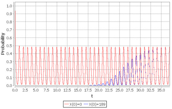
Figure 1. Rate of convergence of the empty system probability $p_0\left(t\right)$ in the interval $[0,37]$ given two different initial conditions: $p_0\left(0\right)=1$ (red line), $p_{189}\left(0\right)=1$ (blue line).

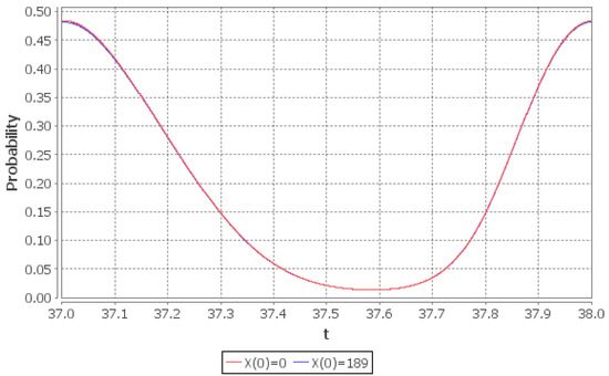
Figure 2. Limiting probability $p_0\left(t\right)$ of the empty queue given two different initial conditions: $p_0\left(0\right)=1$ (red line), $p_{189}\left(0\right)=1$ (blue line).

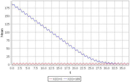
Figure 3. Rate of convergence of the conditional mean $E(t,k)$ number of customers in the system in the interval $[0,37]$: $E(t,0)$ (red line), $E(t,189)$ (blue line).

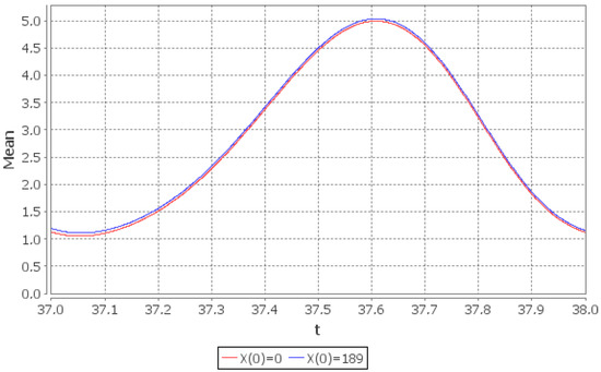
Figure 4. Limiting conditional mean $E(t,k)$ number of customers in the system: $E(t,0)$ (red line), $E(t,189)$ (blue line).

4. Time-Varying Single-Server Markovian System with Bulk Arrivals, Queue Skipping Policy and Catastrophes

Consider the time-varying $M/M/1$ system with the intensities being periodic functions of time and the queue skipping policy as in [31] (see also [32]). Customers arrive to the system in batches according to the inhomogeneous Poisson process with the intensity $\lambda \left(t\right)$. The size of an arriving batch becomes known upon its arrival to the system and is the random variable with the given probability distribution $\{b_n,n\ge 1\}$, having finite mean $\overline{b}={\sum }_{k=1}^{\infty }{B}_k$, $B_k={\sum }_{n=k}^{\infty }{b}_n$. The implemented queue skipping policy implies that whenever a batch arrives to the system its size, say $\widehat{B}$, is compared with the remaining total number of customers in the system, say $\tilde{B}$. If $\widehat{B}>\tilde{B}$, then all customers, that are currently in the system, are instantly removed from it, the whole batch $\widehat{B}$ is placed in the the queue and one customer from it enters server. If $\widehat{B}\le \tilde{B}$ the new batch leaves the system without having any effect on it. Whenever the server becomes free the first customer from the queue (if there is any) enters server and gets served according to the exponential distribution with the intensity $\mu \left(t\right)$. Finally the additional inhomogeneous Poisson flow of negative customers with the intensity $\gamma \left(t\right)$ arrives to the system. Each negative arrival results in the removal of all customers present in the system at the time of arrival. The negative customer itself leaves the system. Since $\gamma \left(t\right)$ depends on t it can happen that the effect of negative arrivals fades away too fast as $t\to \infty$ (for example, if $\gamma \left(t\right)={(1+t)}^{-n}$, $n>1$). Such cases are excluded from the consideration.

Let $X\left(t\right)$ be the total number of customers in the system at time t. From the system description it follows that $X\left(t\right)$ is the CTMC with state space $\{0,1,2,\cdots ,b^{*}\}$, where $b^{*}$ is the maximum possible batch size i.e., $b^{*}={max}_{n\ge 1}(b_n>0)$. Thus if the batch size distribution has infinite support then the state space is countable, otherwise it is finite.

It is straightforward to see that the transposed time-dependent generator $A\left(t\right)={\left(a_{ij}\left(t\right)\right)}_{i,j=0}^{\infty }$ for $X\left(t\right)$ has the form

$$A\left(t\right)=\left(\begin{array}{ccccc}-\lambda \left(t\right)& \mu \left(t\right)+\gamma \left(t\right)& \gamma \left(t\right)& \gamma \left(t\right)& \cdots \\ \lambda \left(t\right)b_1& -\left(\lambda \left(t\right)B_2+\mu \left(t\right)+\gamma \left(t\right)\right)& \mu \left(t\right)& 0& \cdots \\ \lambda \left(t\right)b_2& \lambda \left(t\right)b_2& -\left(\lambda \left(t\right)B_3+\mu \left(t\right)+\gamma \left(t\right)\right)& \mu \left(t\right)& \cdots \\ \lambda \left(t\right)b_3& \lambda \left(t\right)b_3& \lambda \left(t\right)b_3& -\left(\lambda \left(t\right)B_4+\mu \left(t\right)+\gamma \left(t\right)\right)& \cdots \\ ⋮& ⋮& ⋮& ⋮& \ddots \end{array}\right).$$

We represent the distribution of $X\left(t\right)$ as a probability vector $\mathbf{p}\left(t\right)$, where $\mathbf{p}\left(t\right)={\sum }_{k=0}^{b^{*}}\mathsf{P}(X\left(t\right)=k){\mathbf{e}}_k$ tor all $t\ge 0$. Given a proper $\mathbf{p}\left(0\right)$, the probabilistic dynamics of $X\left(t\right)$ is described by the Kolmogorov forward equations $\frac{d}{dt}\mathbf{p}\left(t\right)=A\left(t\right)\mathbf{p}\left(t\right)$, which can be rewritten in the form

$$\frac{d}{dt}\mathbf{p}\left(t\right)=A^{*}\left(t\right)\mathbf{p}\left(t\right)+\mathbf{g}\left(t\right),t\ge 0,$$

(19)

where $\mathbf{g}\left(t\right)={\left(\gamma \left(t\right),0,0,\cdots \right)}^T$ and $A^{*}\left(t\right)$ is the matrix with the terms $a_{ij}^{*}\left(t\right)$ equal to

$$\begin{array}{c}\hfill a_{ij}^{*}\left(t\right)=\left\{\begin{array}{cc}{a}_{0j}\left(t\right)-\gamma \left(t\right),\hfill & \mathrm{if} i=0,\hfill \\ a_{ij}\left(t\right),\hfill & \mathrm{otherwise}.\hfill \end{array}\right.\end{array}$$

(20)

Due to the restrictions imposed on $\gamma \left(t\right)$, we have that ${\int }_0^{\infty }\gamma \left(t\right)dt=\infty$. Thus $X\left(t\right)$ cannot be null ergodic irrespective of the values of $\lambda \left(t\right)$ and $\mu \left(t\right)$.

Theorem 2.

Assume that the catastrophe intensity $\gamma \left(t\right)$ is such that ${\int }_0^{\infty }\gamma \left(t\right)dt=\infty$. Then the Markov chain $X\left(t\right)$ is weakly ergodic and for any two initial conditions ${\mathbf{p}}^{*}\left(0\right)$ and ${\mathbf{p}}^{**}\left(0\right)$ it holds that

$$\begin{array}{c}\hfill ∥{\mathbf{p}}^{*}\left(t\right)-{\mathbf{p}}^{**}\left(t\right)∥\le e^{-\underset{0}{\overset{t}{\int }}\gamma \left(u\right)du}∥{\mathbf{p}}^{*}\left(0\right)-{\mathbf{p}}^{**}\left(0\right)∥\le 2e^{-\underset{0}{\overset{t}{\int }}\gamma \left(u\right)du},t\ge 0.\end{array}$$

(21)

Proof. 

It is straightforward to check, that the logarithmic norm (see (3)) of the operator $A^{*}\left(t\right)$ is equal to $-\gamma \left(t\right)$. Denote now by $U^{*}(t,s)$ the Cauchy operator of the Equation (19). Then the statement of the theorem follows from the inequalities $\parallel U^{*}(t,s)\parallel \le e^{-{\int }_s^t\gamma \left(u\right)du}$ and

$$∥{\mathbf{p}}^{*}\left(t\right)-{\mathbf{p}}^{**}\left(t\right)∥\le ∥U^{*}\left(t,0\right)∥∥{\mathbf{p}}^{*}\left(0\right)-{\mathbf{p}}^{**}\left(0\right)∥.$$

 □

Even though (21) is the valid ergodicity bound for $X\left(t\right)$, it is of little help whenever the state space of $X\left(t\right)$ is countable and one needs to perform the numerical solution of (5). This is due to the fact that the bound (21) is in the uniform operator topology, which does not allow to use the analytic frameworks (for example, [29]) for finding proper truncations of an infinite ODE system. For the latter task ergodicity bounds for $X\left(t\right)$ in stronger (than $l_1$), weighted norms are required. It can be said that with such bounds we have a weight assigned to each initial state and thus a truncation procedure becomes sensitive to the number of states. Below (in the Theorem 3) we obtain such a bound under the additional assumption, (for the definition used see [33]; appropriate test for monotone functions can be found in [Proposition 1] of [34]. Although the Theorem 2 below holds for any distribution $\{b_n,n\ge 1\}$, this assumption is essential for the Theorem 3. For distributions with tails heavier than the geometric distribution we were unable to find the conditions, which guarantee the existence of the limiting regime of queue-size process even for periodic intensities). that the batch size distribution $\{b_n,n\ge 1\}$ is harmonic new better than used in expectation i.e., ${\sum }_{j=k}^{\infty }{B}_{j+1}\le \overline{b}{\left(1-{\overline{b}}^{-1}\right)}^k$ for all $k\ge 0$.

Using the normalization condition $p_0\left(t\right)=1-{\sum }_{i\ge 1}{p}_i\left(t\right)$ the forward Kolmogorov system $\frac{d}{dt}\mathbf{p}\left(t\right)=A\left(t\right)\mathbf{p}\left(t\right)$ can be rewritten as

$$\frac{d}{dt}\mathbf{z}\left(t\right)=A^{**}\left(t\right)\mathbf{z}\left(t\right)+\mathbf{f}\left(t\right),t\ge 0,$$

(22)

where

$\mathbf{f}\left(t\right)={\left(\lambda \left(t\right)b_1,\lambda \left(t\right)b_2,\lambda \left(t\right)b_3,\lambda \left(t\right)b_4,\cdots \right)}^T$ and

$$A^{**}\left(t\right)=\left(\begin{array}{ccccc}-\left(\lambda \left(t\right)+\mu \left(t\right)+\gamma \left(t\right)\right)& \mu \left(t\right)-\lambda \left(t\right)b_1& -\lambda \left(t\right)b_1& -\lambda \left(t\right)b_1& \cdots \\ 0& -\left(\lambda \left(t\right)B_2+\mu \left(t\right)+\gamma \left(t\right)\right)& \mu \left(t\right)-\lambda \left(t\right)b_2& -\lambda \left(t\right)b_2& \cdots \\ 0& 0& -\left(\lambda \left(t\right)B_3+\mu \left(t\right)+\gamma \left(t\right)\right)& \mu \left(t\right)-\lambda \left(t\right)b_3& \cdots \\ 0& 0& 0& -\left(\lambda \left(t\right)B_4+\mu \left(t\right)+\gamma \left(t\right)\right)& \cdots \\ ⋮& ⋮& ⋮& ⋮& \ddots \end{array}\right).$$

(23)

Fix $d\in (1,1+{(\overline{b}-1)}^{-1}]$ and define the increasing sequence of positive numbers $\{{\delta }_n,n\ge 0\}$ by ${\delta }_n=d^{n-1}$. Then instead of the matrix $B^{**}\left(t\right)$ in (13) we have the matrix $\tilde{A}\left(t\right)={\left({\tilde{a}}_{ij}\left(t\right)\right)}_{i,j=0}^{\infty }$ with the following structure:

$$\tilde{A}\left(t\right)=\left(\begin{array}{ccccc}-\left(\lambda \left(t\right)+\mu \left(t\right)+\gamma \left(t\right)\right)& \frac{1}{d}\mu \left(t\right)& 0& 0& \cdots \\ 0& -\left(\lambda \left(t\right)B_2+\mu \left(t\right)+\gamma \left(t\right)\right)& \frac{1}{d}\mu \left(t\right)& 0& \cdots \\ 0& 0& -\left(\lambda \left(t\right)B_3+\mu \left(t\right)+\gamma \left(t\right)\right)& \frac{1}{d}\mu \left(t\right)& \cdots \\ 0& 0& 0& -\left(\lambda \left(t\right)B_4+\mu \left(t\right)+\gamma \left(t\right)\right)& \cdots \\ ⋮& ⋮& ⋮& ⋮& \ddots \end{array}\right).$$

(24)

Since the logarithmic norm (see (3)) of $\tilde{A}\left(t\right)$ is equal to

$$\begin{array}{c}-{\beta }^{*}\left(t\right)=\underset{i}{sup}\left\{{\tilde{a}}_{ii}\left(t\right)+\sum _{j\ne i}{\tilde{a}}_{ji}\left(t\right)\right\}=-\underset{i}{inf}\left\{\gamma \left(t\right)+\left(1-\frac{1}{d}\right)\mu \left(t\right)+\lambda \left(t\right)B_i\right\}\hfill \\ \hfill =-\gamma \left(t\right)-\left(1-\frac{1}{d}\right)\mu \left(t\right),\end{array}$$

then from (4) we get:

$$\begin{array}{c}\hfill {∥{\mathbf{z}}^{*}\left(t\right)-{\mathbf{z}}^{**}\left(t\right)∥}_{1\mathsf{D}}\le e^{-\underset{0}{\overset{t}{\int }}\left(\gamma \left(u\right)+\left(1-d^{-1}\right)\mu \left(u\right)\right)du}{∥{\mathbf{z}}^{*}\left(0\right)-{\mathbf{z}}^{**}\left(0\right)∥}_{1\mathsf{D}}.\end{array}$$

(25)

Arguments similar to those used to establish the Theorem 1 lead to the following ergodicity bounds for $\parallel {\mathbf{p}}^{*}\left(t\right)-{\mathbf{p}}^{**}\left(t\right)\parallel$ and the conditional mean $E(t,k)$:

$$∥{\mathbf{p}}^{*}\left(t\right)-{\mathbf{p}}^{**}\left(t\right)∥\le 4e^{-\underset{0}{\overset{t}{\int }}\left(\gamma \left(u\right)+\left(1-d^{-1}\right)\mu \left(u\right)\right)du}{∥{\mathbf{z}}^{*}\left(0\right)-{\mathbf{z}}^{**}\left(0\right)∥}_{1\mathsf{D}},$$

(26)

$$|E(t,k)-E(t,0)|\le \frac{1+d^{k-1}}{W}{e}^{-\underset{0}{\overset{t}{\int }}\left(\gamma \left(u\right)+\left(1-d^{-1}\right)\mu \left(u\right)\right)du},k\ge 1,W=\underset{n}{inf}\frac{d^n}{n+1}.$$

(27)

These results can be put together in the single theorem.

Theorem 3.

Assume that the distribution $\{b_n,n\ge 1\}$ with finite mean $\overline{b}$ is harmonic new better than used in expectation. Then if ${\int }_0^{\infty }\left(\gamma \left(t\right)+(1-d^{-1})\mu \left(t\right)\right)dt=+\infty$ for some $d\in (1,1+{(\overline{b}-1)}^{-1}]$, then the Markov chain $X\left(t\right)$ is weakly ergodic and the ergodicity bound (26) holds.

We close this section with the example, showing the dependence on t of the same two quantities — $p_0\left(t\right)$ and $E(t,k)$—considered in the Section 3. Assume here that $b_k=\frac{1}{3}{\left(\frac{2}{3}\right)}^{k-1}$, $\lambda \left(t\right)=9\left(1+sin2\pi t\right)$, $\mu \left(t\right)=8\left(1+cos2\pi t\right)$ and $\gamma \left(t\right)=1$, i.e., the catastrophe intensity is constant and the mean size $\overline{b}$ of an arriving batch is equal to 3. It can be checked that $d=\frac{3}{2}$ satisfies the conditions of the Theorem 3. Then from (26) and (27) we get the upper bounds

$$∥{\mathbf{p}}^{*}\left(t\right)-{\mathbf{p}}^{**}\left(t\right)∥\le 4e^{-\frac{5}{3}t}{∥{\mathbf{z}}^{*}\left(0\right)-{\mathbf{z}}^{**}\left(0\right)∥}_{1D},$$

(28)

$$|E(t,k)-E(t,0)|\le \frac{1+{\left(\frac{3}{2}\right)}^{k-1}}{\frac{9}{8}}{e}^{-\frac{5}{3}t},k\ge 0.$$

(29)

In Figure 5 it is depicted how $p_0\left(t\right)$ behaves as t increases and Figure 6 shows its limiting value. If $t\ge 60$ then the right part of (28) does not exceed $3·{10}^{-2}$, i.e., starting from the instant $t=60=t^{*}$ the system “forgets” its initial state and the distribution of $X\left(t\right)$ for $t>t^{*}$ can be regarded as limiting. Moreover, since the limiting distribution of $X\left(t\right)$ is periodic, it is sufficient to solve (numerically, (it must be noticed that since $b_k>0$ for all k, the system of ODEs contains infinite number of equations. Thus in order to solve it numerically one has to truncate it. We perform this truncation according to the method in [30])). the system of ODEs only in the interval $[0,t^{*}+T]$, where T is the smallest common multiple of the periods of $\lambda \left(t\right)$ and $\mu \left(t\right)$ i.e., $T=1$. The probability distribution of $X\left(t\right)$ in the interval $[t^{*},t^{*}+T]$ is the estimate (with error not greater than $3·{10}^{-2}$ in $l_1$-norm) of the limiting probability distribution of $X\left(t\right)$. The upper bound on the rate of convergence of the conditional mean number of customers in the system $E(t,k)$ is given in (29). If $t\ge t^{*}$ then the right part does not exceed $0,3$, i.e., starting from the instant $t=t^{*}$ the system “forgets” its initial state and the value of $E(t,k)$ can be regarded as the limiting value of the mean number of customers with the error not greater than $0,3$. The rate of convergence of $E(t,k)$ and the behaviour of its limiting value can be seen in Figure 7 and Figure 8. As in the previous numerical example, the obtained upper bounds are not tight: the system enters the periodic limiting regime before the instant $t=t^{*}$.

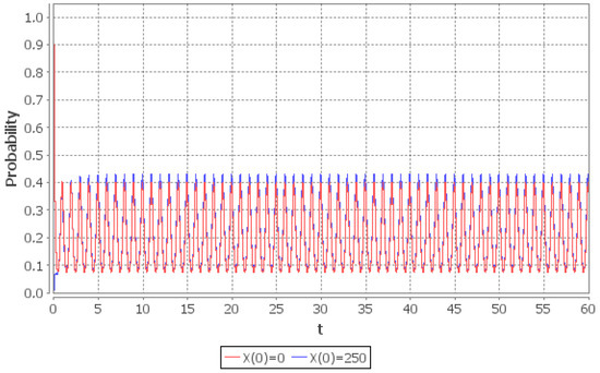
Figure 5. Rate of convergence of the empty system probability $p_0\left(t\right)$ in the interval $[0,60]$ given two different initial conditions: $p_0\left(0\right)=1$ (red line), $p_{250}\left(0\right)=1$ (blue line).

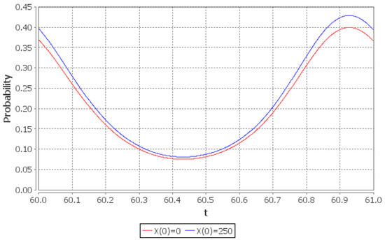
Figure 6. Limiting probability $p_0\left(t\right)$ of the empty queue given two different initial conditions: $p_0\left(0\right)=1$ (red line), $p_{250}\left(0\right)=1$ (blue line).

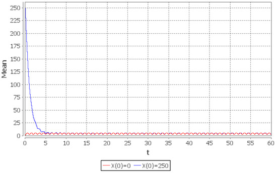
Figure 7. Rate of convergence of the conditional mean $E(t,k)$ number of customers in the system in the interval $[0,60]$: $E(t,0)$ (red line), $E(t,250)$ (blue line).

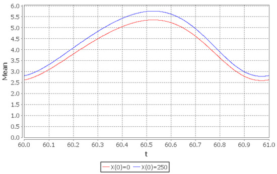
Figure 8. Limiting conditional mean $E(t,k)$ number of customers in the system: $E(t,0)$ (red line), $E(t,250)$ (blue line).

5. Time-Varying Markovian Bulk-Arrival and Bulk-Service System with State-Dependent Control

In the recent paper [35] the authors considered the Markovian bulk-arrival and bulk-service system with the general state-dependent control (see also [35,36,37,38,39]). The total number $X\left(t\right)$ of customers at time t in that system constitutes CTMC with state space $\{0,1,2,\cdots \}$. Its generator $Q\left(t\right)={\left(q_{ij}\left(t\right)\right)}_{i,j=0}^{\infty }$ has quite a specific structure:

$$q_{ij}=\left\{\begin{array}{cc}{h}_{ij},\hfill & \mathrm{if} 0\le i\le k-1,j\ge 0,\hfill \\ b_{i-j+k},\hfill & \mathrm{if} i\ge k,j\ge i-k,\hfill \\ 0,\hfill & \mathrm{otherwise},\hfill \end{array}\right.$$

(30)

where $k\ge 1$ is the fixed integer. For further explanations and the motivation behind such structure of $Q\left(t\right)$ we refer the reader to [Section 1] in [35]. The purpose of this section is to show that for at least one particular case of this system, even when the intensities are time-dependent, one can obtain the upper bounds for the rate of convergence using the method based on the logarithmic norm. Specifically, we take the example, (in the example of [Section 7] in [35] the entries of the intensity matrix $Q\left(t\right)$ are: $h_{i,i-1}=\mu$, $h_{i,i+1}=\lambda$, $h_{i,i}=-(\lambda +\mu )$, $b_0=a$, $b_{k+1}=b$, $b_k=-(a+b)$ and $k=3$). from the Section 7 of [35], with the exception that all the transition intensities are time-dependent i.e., $b_i=\lambda \left(t\right)$ and $a_i=\mu \left(t\right)$ and are both nonnegative locally integrable on $[0,\infty )$. Then the transposed generator $A\left(t\right)={\left(a_{ij}\left(t\right)\right)}_{i,j=0}^{\infty }=Q^T\left(t\right)$ of $X\left(t\right)$ has the form

$$\begin{array}{c}\hfill A\left(t\right)=\left(\begin{array}{ccccccc}-\lambda \left(t\right)& \mu \left(t\right)& 0& \mu \left(t\right)& 0& 0& \cdots \\ \lambda \left(t\right)& -\left(\lambda \right(t)+\mu (t\left)\right)& \mu \left(t\right)& 0& \mu \left(t\right)& 0& \cdots \\ 0& \lambda \left(t\right)& -\left(\lambda \right(t)+\mu (t\left)\right)& 0& 0& \mu \left(t\right)& \cdots \\ 0& 0& \lambda \left(t\right)& -\left(\lambda \right(t)+\mu (t\left)\right)& 0& 0& \cdots \\ 0& 0& 0& \lambda \left(t\right)& -\left(\lambda \right(t)+\mu (t\left)\right)& 0& \cdots \\ 0& 0& 0& 0& \lambda \left(t\right)& -\left(\lambda \right(t)+\mu (t\left)\right)& \cdots \\ ⋮& ⋮& ⋮& ⋮& ⋮& ⋮& \ddots \end{array}\right)\end{array}$$

(31)

Denote the distribution of $X\left(t\right)$ by $\mathbf{p}\left(t\right)$ i.e., $\mathbf{p}\left(t\right)={(p_0\left(t\right),p_1\left(t\right),\cdots )}^{\mathrm{T}}={\sum }_{k=0}^{\infty }\mathsf{P}$

$(X\left(t\right)=k){\mathbf{e}}_k$ (as above, ${\mathbf{e}}_k$ denotes the kth unit basis vector). The ergodicity bound for $X\left(t\right)$ in the null ergodic case is given below in the Theorem 4.

Theorem 4.

If ${\int }_0^{\infty }\left(\lambda \left(t\right)(1-\sigma )+\mu \left(t\right)(1-{\sigma }^{-3})\right)dt=+\infty$ for some $\sigma \in (0,1)$, then the Markov chain $X\left(t\right)$ is null ergodic,

$$\sum _{i=0}^{\infty }{\sigma }^i{p}_i\left(t\right)\le e^{-{\int }_0^t\left(\lambda \left(u\right)+\mu \left(u\right)-\sigma \lambda \left(u\right)-{\sigma }^{-3}\mu \left(u\right)\right)du}\sum _{i=0}^{\infty }{\sigma }^i{p}_i\left(0\right),t\ge 0,$$

(32)

and for any $n\ge 0$ and $N\ge 0$ the following inequality holds:

$$\mathsf{P}\left(X\left(t\right)>n\left|X\right(0)=N\right)\ge 1-{\sigma }^{N-n}{e}^{-{\int }_0^t\left(\lambda \left(u\right)+\mu \left(u\right)-\sigma \lambda \left(u\right)-{\sigma }^{-3}\mu \left(u\right)\right)du}.$$

(33)

Proof. 

Fix $\sigma >0$ and define the decreasing sequence of positive numbers $\{{\delta }_n,n\ge 0\}$ by ${\delta }_n={\sigma }^n$. Put $\tilde{\mathbf{p}}\left(t\right)=\mathsf{\Lambda }\mathbf{p}\left(t\right)$, where $\mathsf{\Lambda }=diag\left({\delta }_0,{\delta }_1,\cdots \right)$. Then we have (6). Denote by $-{\tilde{\alpha }}_k\left(t\right)$ the sum of all elements in the kth column of $\tilde{A}\left(t\right)$ i.e.

$$\begin{array}{ccc}\hfill {\tilde{\alpha }}_0\left(t\right)& =& \left(1-\sigma \right)\lambda \left(t\right),\hfill \\ \hfill {\tilde{\alpha }}_k\left(t\right)& =& \left(1-\sigma \right)\left(\lambda \left(t\right)+\mu \left(t\right)-{\sigma }^{-1}\mu \left(t\right)\right),k=1,2,\hfill \\ \hfill {\tilde{\alpha }}_k\left(t\right)& =& \underset{=\beta \left(t\right)}{\underbrace{\lambda \left(t\right)+\mu \left(t\right)-\sigma \lambda \left(t\right)-{\sigma }^{-3}\mu \left(t\right)}},k\ge 3.\hfill \end{array}$$

If $0<\sigma <1$ then ${\tilde{\alpha }}_0\left(t\right)\ge \beta \left(t\right)$, ${\tilde{\alpha }}_1\left(t\right)\ge \beta \left(t\right)$ and ${\tilde{\alpha }}_2\left(t\right)\ge \beta \left(t\right)$, and thus (32) and (33) follow from (4) and (8) respectively. □

The ergodicity bound in the weakly ergodic case, state below in the Theorem 5, is obtained by analogy with the Theorem 1. Define an increasing sequence of positive numbers $\{{\delta }_n,n\ge 0\}$. Then the matrix $B^{**}\left(t\right)$ built from the matrix $A\left(t\right)$, in the same way as it is done in the Section 3, has the form:

$$\begin{array}{c}\hfill B^{**}\left(t\right)=\left(\begin{array}{ccccccc}-\left(\lambda \right(t)+\mu (t\left)\right)& \mu \left(t\right)\frac{{\delta }_1}{{\delta }_2}& -\mu \left(t\right)\frac{{\delta }_1}{{\delta }_3}& \mu \left(t\right)\frac{{\delta }_1}{{\delta }_4}& 0& 0& \cdots \\ \lambda \left(t\right)\frac{{\delta }_2}{{\delta }_1}& -\left(\lambda \right(t)+\mu (t\left)\right)& 0& 0& \mu \left(t\right)\frac{{\delta }_2}{{\delta }_5}& 0& \cdots \\ 0& \lambda \left(t\right)\frac{{\delta }_3}{{\delta }_2}& -\left(\lambda \right(t)+\mu (t\left)\right)& 0& 0& \mu \left(t\right)\frac{{\delta }_3}{{\delta }_6}& \cdots \\ 0& 0& \lambda \left(t\right)\frac{{\delta }_4}{{\delta }_3}& -\left(\lambda \right(t)+\mu (t\left)\right)& 0& 0& \cdots \\ 0& 0& 0& \lambda \left(t\right)\frac{{\delta }_5}{{\delta }_4}& -\left(\lambda \right(t)+\mu (t\left)\right)& 0& \cdots \\ 0& 0& 0& 0& \lambda \left(t\right)\frac{{\delta }_6}{{\delta }_5}& -\left(\lambda \right(t)+\mu (t\left)\right)& \cdots \\ ⋮& ⋮& ⋮& ⋮& ⋮& ⋮& \ddots \end{array}\right)\end{array}$$

(34)

Denote by $-{\tilde{\alpha }}_k\left(t\right)$ the sum of all elements in the kth column of $B^{**}\left(t\right)$ i.e.,

$$\begin{array}{ccc}\hfill {\alpha }_1\left(t\right)& =& \lambda \left(t\right)+\mu \left(t\right)-\lambda \left(t\right)\frac{{\delta }_2}{{\delta }_1},\hfill \\ \hfill {\alpha }_2\left(t\right)& =& \lambda \left(t\right)+\mu \left(t\right)-\lambda \left(t\right)\frac{{\delta }_3}{{\delta }_2}-\mu \left(t\right)\frac{{\delta }_1}{{\delta }_2},\hfill \\ \hfill {\alpha }_3\left(t\right)& =& \lambda \left(t\right)+\mu \left(t\right)-\lambda \left(t\right)\frac{{\delta }_4}{{\delta }_3}-\mu \left(t\right)\frac{{\delta }_1}{{\delta }_3},\hfill \\ \hfill {\alpha }_k\left(t\right)& =& \lambda \left(t\right)+\mu \left(t\right)-\lambda \left(t\right)\frac{{\delta }_{k+1}}{{\delta }_k}-\mu \left(t\right)\frac{{\delta }_{k-3}}{{\delta }_k},k\ge 4.\hfill \end{array}$$

Since the logarithmic norm of $B^{**}\left(t\right)$ is equal to $-\beta \left(t\right)=-min\left({min}_{1\le k\le 3}{\alpha }_k\left(t\right),{inf}_{k\ge 4}{\alpha }_k\left(t\right)\right)$, we can apply (4) to (13) and (15) with ${\delta }_{k+1}=\sigma {\delta }_k$, $k\ge 5$.

Theorem 5.

If ${\int }_0^{\infty }\left(\lambda \left(t\right)(1-\sigma )+\mu \left(t\right)(1-{\sigma }^{-3})\right)dt=+\infty$ for some $\sigma >0$, then the Markov chain $X\left(t\right)$ is weakly ergodic and the ergodicity bound (15) holds.

As the numerical example we again consider the periodic case: $\lambda \left(t\right)=3\left(1+sin\pi t\right)$ and $\mu \left(t\right)=4\left(1+cos2\pi t\right)$. By direct inspection it can be checked that the sequence $\{{\delta }_n,n\ge 1\}$, defined by ${\delta }_n={\frac{10}{9}}^{n-1}$, leads to $\beta \left(t\right)={\alpha }_2\left(t\right)$. Thus the conditions of the Theorem 5 are fulfilled with $\sigma =\frac{10}{9}$. The pre-limiting and the limiting values of the same quantities as in the two previous examples—$p_0\left(t\right)$ and $E(t,k)$—are shown in Figure 9, Figure 10, Figure 11 and Figure 12.

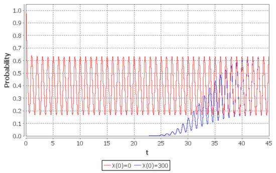
Figure 9. Rate of convergence of the empty system probability $p_0\left(t\right)$ in the interval $[0,45]$ given two different initial conditions: $p_0\left(0\right)=1$ (red line), $p_{250}\left(0\right)=1$ (blue line).

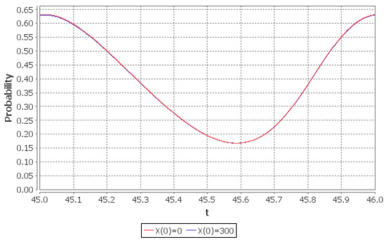
Figure 10. Limiting probability $p_0\left(t\right)$ of the empty queue given two different initial conditions: $p_0\left(0\right)=1$ (red line), $p_{300}\left(0\right)=1$ (blue line).

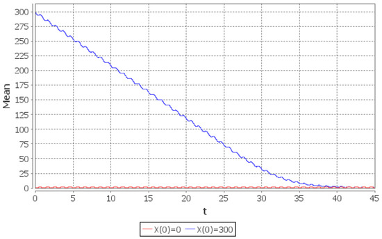
Figure 11. Rate of convergence of the conditional mean $E(t,k)$ number of customers in the system in the interval $[0,45]$: $E(t,0)$ (red line), $E(t,300)$ (blue line).

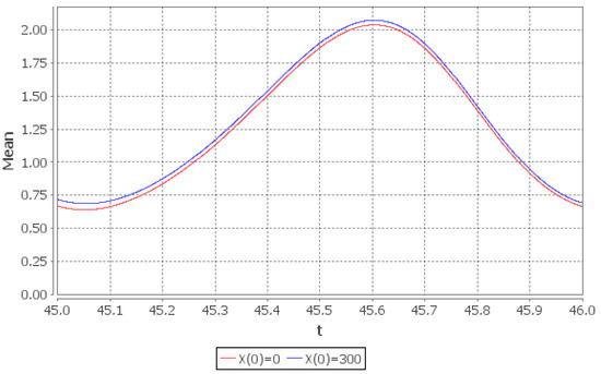
Figure 12. Limiting conditional mean $E(t,k)$ number of customers in the system: $E(t,0)$ (red line), $E(t,300)$ (blue line).

6. Conclusions

As can be seen from the last three sections, in order to obtain the ergodicity bounds the values of $\lambda \left(t\right)$ and $\mu \left(t\right)$ for each t may not be needed. Instead it may be sufficient to know only the time-average intensities $\overline{\lambda }=\frac{1}{t}{lim}_{t\to \infty }{\int }_0^t\lambda \left(u\right)du$ and $\overline{\mu }=\frac{1}{t}{lim}_{t\to \infty }{\int }_0^t\mu \left(u\right)du$. For periodic intensities with the smallest common multiple of the periods T, the values $\overline{\lambda }$ and $\overline{\mu }$ are exactly the average arrival and service intensity over one period.

The classes of CTMC to which the logarithmic norm method is applicable and gives meaningful results is not limited to those considered in this paper, (necessary and sufficient conditions for a CTMC “to fit” the logarithmic norm method are not known). For example, the same reasoning, which has led to the Theorem 1, can be used to obtain the upper bounds for the rate of convergence of the $M_t/M_t/S/\infty$ system with any (finite) number of servers. Moreover, whenever $X\left(t\right)$ is weakly ergodic, the analysis can be carried on beyond what is stated in the Theorem 1. For example, one can obtain the perturbation bounds (see e.g., [40]) and study different state space truncation options: one-sided or two sided (see e.g., [29,41,42]).

References

- Liu, Y.; Whitt, W. Stabilizing performance in a service system with time-varying arrivals and customer feedback. Eur. J. Oper. Res. 2017, 256, 473–486. [Google Scholar] [CrossRef]
- Liu, Y. Staffing to stabilize the tail probability of delay in service systems with time-varying demand. Oper. Res. 2018, 66, 514–534. [Google Scholar] [CrossRef]
- Kwon, S.; Gautam, N. Guaranteeing performance based on time-stability for energy-efficient data centers. IIE Trans. 2016, 48, 812–825. [Google Scholar] [CrossRef]
- Whitt, W.; You, W. Time-Varying Robust Queueing; Columbia University: New York, NY, USA, 2019. [Google Scholar]
- Schwarz, J.A.; Selinka, G.; Stolletz, R. Performance analysis of time-dependent queueing systems: Survey and classification. Omega 2016, 63, 170–189. [Google Scholar] [CrossRef]
- Whitt, W. Time-Varying Queues. Available online: http://www.columbia.edu/~ww2040/TVQ_082617.pdf (accessed on 28 October 2020).
- Falin, G.I. Periodic queues in heavy traffic. Adv. Appl. Probab. 1989, 21, 485–487. [Google Scholar] [CrossRef][Green Version]
- Masuyama, H. Error bounds for augmented truncations of discrete-time block-monotone Markov chains under geometric drift conditions. Adv. Appl. Probab. 2015, 47, 83–105. [Google Scholar] [CrossRef]
- Tweedie, R.L. Truncation approximations of invariant measures for Markov chains. J. Appl. Probab. 1998, 35, 517–536. [Google Scholar] [CrossRef]
- Green, L.; Kolesar, P. The pointwise stationary approximation for queues with nonstationary arrivals. Manag. Sci. 1991, 37, 84–97. [Google Scholar] [CrossRef]
- Di Crescenzo, A.; Nobile, A.G. Diffusion approximation to a queueing system with time-dependent arrival and service rates. Queueing Syst. 1995, 19, 41–62. [Google Scholar] [CrossRef]
- Di Crescenzo, A.; Giorno, V.; Nobile, A.G.; Ricciardi, L.M. On the M/M/1 queue with catastrophes and its continuous approximation. Queueing Syst. 2003, 43, 329–347. [Google Scholar] [CrossRef]
- Kolesar, P.J.; Rider, P.J.; Craybill, T.B.; Walker, W.E. A queueing linear-programming approach to scheduling police patrol cars. Oper. Res. 1975, 23, 1045–1062. [Google Scholar] [CrossRef]
- Taaffe, M.R.; Ong, K.L. Approximating Nonstationary Ph(t)/M(t)/s/c queueing systems. Ann. Oper. Res. 1987, 8, 103–116. [Google Scholar] [CrossRef]
- Clark, G.M. Use of Polya distributions in approximate solutions to nonstationary M/M/s queues. Commun. ACM 1981, 24, 206–217. [Google Scholar] [CrossRef]
- Massey, W.; Pender, J. Gaussian skewness approximation for dynamic rate multiserver queues with abandonment. Queueing Syst. 2013, 75, 243–327. [Google Scholar] [CrossRef]
- Van Dijk, N.M.; van Brummelen, S.P.J.; Boucherie, R.J. Uniformization: Basics, extensions and applications. Perform. Eval. 2018, 118, 8–32. [Google Scholar] [CrossRef]
- Arns, M.; Buchholz, P.; Panchenko, A. On the numerical analysis of inhomogeneous continuous-time Markov chains. Informs J. Comput. 2010, 22, 416–432. [Google Scholar] [CrossRef]
- Andreychenko, A.; Sandmann, W.; Wolf, V. Approximate adaptive uniformization of continuous-time Markov chains. Appl. Math. Model. 2018, 61, 561–576. [Google Scholar] [CrossRef]
- Burak, M.R.; Korytkowski, P. Inhomogeneous CTMC Birth-and-Death Models Solved by Uniformization with Steady-State Detection. ACM Trans. Model. Comput. Simul. 2020, 30, 1–18. [Google Scholar] [CrossRef]
- Burak, M.R. Efficiency Improvements to Uniformization for Markovian Birth-and-Death Models. In Proceedings of the 2018 23rd International Conference on Methods & Models in Automation & Robotics (MMAR), Miedzyzdroje, Poland, 27–30 August 2018; pp. 741–746. [Google Scholar]
- Ingolfsson, A.; Akhmetshina, E.; Budge, S.; Li, Y.; Wu, X. A survey and experimental comparison of service-level-approximation methods for nonstationary M (t)/M/s (t) queueing systems with exhaustive discipline. Informs J. Comput. 2007, 19, 201–214. [Google Scholar] [CrossRef]
- Li, Y.F.; Zio, E.; Lin, Y.H. Methods of solutions of inhomogeneous continuous time Markov chains for degradation process modeling. Appl. Reliab. Eng. Risk Anal. Probab. Models Stat. Inference 2013, 3–16. [Google Scholar] [CrossRef]
- Katoen, J.-P.; Zapreev, I.S. Safe on-the-fly steady-state detection for time-bounded reachability. In Proceedings of the 3rd International Conference on the Quantitative Evaluation of Systems, California, CA, USA, 11–14 September 2016. [Google Scholar]
- Down, D.; Meyn, S.P.; Tweedie, R.L. Exponential and uniform ergodicity of Markov processes. Ann. Probab. 1995, 23, 1671–1691. [Google Scholar] [CrossRef]
- Meyn, S.P.; Tweedie, R.L. Markov Chains and Stochastic Stability; Springer Science and Business Media: New York, NY, USA, 2012. [Google Scholar]
- Zeifman, A.; Satin, Y.; Kiseleva, K.; Korolev, V. On the Rate of Convergence for a Characteristic of Multidimensional Birth-Death Process. Mathematics 2019, 7, 477. [Google Scholar] [CrossRef]
- Zeifman, A.; Satin, Y.; Kryukova, A.; Razumchik, R.; Kiseleva, K.; Shilova, G. On Three Methods for Bounding the Rate of Convergence for Some Continuous-Time Markov Chains. Int. J. Appl. Math. Comput. Sci. 2020, 30, 251–266. [Google Scholar]
- Zeifman, A.; Satin, Y.; Korolev, V.; Shorgin, S. On truncations for weakly ergodic inhomogeneous birth and death processes. Int. J. Appl. Math. Comput. Sci. 2014, 24, 503–518. [Google Scholar] [CrossRef]
- Zeifman, A.I.; Korotysheva, A.; Satin, Y.; Kiseleva, K.; Korolev, V.; Shorgin, S. Bounds for Markovian Queues With Possible Catastrophes. In Proceedings of the 31st Conference on Modelling and Simulation, Budapest, Hungary, 23–26 May 2017; pp. 628–634. [Google Scholar]
- Marin, A.; Rossi, S. A Queueing Model that Works Only on the Biggest Jobs. Lect. Notes Comput. Sci. Book Ser. 2020, 12039, 118–132. [Google Scholar]
- Zeifman, A.; Razumchik, R.; Satin, Y.; Kovalev, I. Ergodicity Bounds for the Markovian Queue With Time-Varying Transition Intensities, Batch Arrivals and One Queue Skipping Policy. arXiv 2020, arXiv:2007.15833. [Google Scholar]
- Klefsjö, B. The hnbue and hnwue classes of life distributions. Nav. Res. Logist. 1982, 29, 331–344. [Google Scholar] [CrossRef]
- Conti, P.L.J. An asymptotic test for a geometric process against a lattice distribution with monotone hazard. Ital. Statist. Soc. 1997, 6, 213–231. [Google Scholar] [CrossRef]
- Chen, A.; Wu, X.; Zhang, J. Markovian bulk-arrival and bulk-service queues with general state-dependent control. Queueing Syst. 2020, 1–48. [Google Scholar] [CrossRef]
- Chen, A.; Renshaw, E. Markovian bulk-arriving queues with state-dependent control at idle time. Adv. Appl. Probab. 2004, 36, 499–524. [Google Scholar] [CrossRef]
- Chen, A.; Pollett, P.; Li, J.; Zhang, H. Markovian bulk-arrival and bulk-service queues with state-dependent control. Queueing Syst. 2010, 64, 267–304. [Google Scholar] [CrossRef]
- Chen, A.; Li, J.; Hou, Z.; Ng, K.W. Decay properties and quasi-stationary distributions for stopped Markovian bulk-arrival and bulk-service queues. Queueing Syst. 2010, 66, 275–311. [Google Scholar] [CrossRef][Green Version]
- Li, J.; Chen, A. Decay property of stopped Markovian bulk-arriving queues. Adv. Appl. Probab. 2008, 40, 95–121. [Google Scholar] [CrossRef]
- Zeifman, A.; Korolev, V.; Satin, Y. Two approaches to the construction of perturbation bounds for continuous-time Markov chains. Mathematics 2020, 8, 253. [Google Scholar] [CrossRef]
- Satin, Y.; Kiseleva, K.; Shorgin, S.; Korolev, V.; Zeifman, A. Two-Sided Truncations for The Mt/Mt/S Queueing Model. In Proceedings of the 31st European Conference on Modelling and Simulation, Budapest, Hungary, 23–26 May 2017; pp. 635–641. [Google Scholar]
- Zeifman, A.; Leorato, S.; Orsingher, E.; Satin, Y.; Shilova, G. Some universal limits for nonhomogeneous birth and death processes. Queueing Syst. 2006, 52, 139–151. [Google Scholar] [CrossRef]
Publisher’s Note: MDPI stays neutral with regard to jurisdictional claims in published maps and institutional affiliations. |
© 2020 by the authors. Licensee MDPI, Basel, Switzerland. This article is an open access article distributed under the terms and conditions of the Creative Commons Attribution (CC BY) license (http://creativecommons.org/licenses/by/4.0/).