A Nonlinear Model Predictive Control with Enlarged Region of Attraction via the Union of Invariant Sets

Abstract

In the dual-mode model predictive control (MPC) framework, the size of the stabilizable set, which is also the region of attraction, depends on the terminal constraint set. This paper aims to formulate a larger terminal set for enlarging the region of attraction in a nonlinear MPC. Given several control laws and their corresponding terminal invariant sets, a convex combination of the given sets is used to construct a time-varying terminal set. The resulting region of attraction is the union of the regions of attraction from each invariant set. Simulation results show that the proposed MPC has a larger stabilizable initial set than the one obtained when a fixed terminal set is used.

1. Introduction

Model predictive control (MPC) is an optimal controller that minimizes a cost index over a finite horizon implemented in the receding horizon framework. The advantage of MPC over conventional controllers is the ability to handle the state and control constraints. When the state is measured at a sampling time, an optimization problem is solved. However, only the first element of the optimal solution is applied to the system. Then, the whole procedure is repeated at the next sampling time [1].

The concept of a dual-mode MPC is widely used to guarantee the stability of MPC for both linear systems, e.g., [2,3], and nonlinear systems, e.g., [4,5,6]. The terminal penalty function is used as an upper bound of the infinite horizon cost needed to drive the state trajectory to the origin when the initial condition is in the terminal region. Moreover, closed-loop stability is ensured by forcing the terminal state to belong to a feasible and invariant set. Hence, the region of attraction is the set of initial conditions that can be steered to the terminal region in N steps or less, where N is the prediction horizon. In other words, it is a N-steps stabilizable set. Several studies have been devoted to formulate a terminal set that makes the region of attraction as large as possible. By increasing the prediction horizon, the domain of attraction can be enlarged at the expense of more computational effort due to the increasing number of decision variables [7]. Hence, in the literature, various approaches have been proposed to enlarge the region of attraction through a larger terminal set. In [8], it is shown that the saturated local control law is used to yield a considerably larger terminal constraint set. A sequence of sets is used in [9] to replace a single terminal set. The contractive set does not need to be invariant as long as there is an admissible control that eventually steers the states to an invariant set. Hence, a larger domain of attraction can be obtained by extending the sequence with a reachable set. In [10], the terminal constraint is only applied to the unstable states, giving the flexibility to have a larger set. A linear time-varying MPC is mostly used to extend a linear MPC with an enlarged terminal set for a nonlinear system, e.g., in [11,12,13,14].

Interpolation-based MPC for a linear system is studied by [15,16] to achieve a compromise between the size of domain attraction and the optimality. The MPC is designed by selecting several invariant sets and expressing the terminal state as a convex combination of states belonging to the invariant sets. By doing that, the resulting terminal set becomes the convex hull of the predefined-invariant sets. For reducing the number of decision variables, the interpolation method can be implicitly employed, meaning that the terminal state is not explicitly expressed as the convex combination of several states but is still the convex hull of several invariant sets, e.g., in [17,18]. The design procedure starts by designing several stabilizing feedback control gains $K_i,i=1,\dots ,m,$ for a given linear time-invariant system. Then, feasible and invariant ellipsoids ${\mathcal{E}}_i=\{x|x^T{R}_i^{-1}x\le 1\}$, $R_i>0$, are defined such that some necessary linear matrix inequalities (LMIs) are satisfied for each matrix $R_i,i\in [1,m]$. These LMIs are popularly used to show that ${\mathcal{E}}_i$ can be applied as the terminal set for a linear MPC [19]. It is then shown that applying a convex combination to the m given LMIs yields a new LMI. As a result, the set ${\mathcal{E}}_{\mathbf{\lambda }}=\{x|x^T{({\sum }_{i=1}^m{\lambda }_i{R}_i)}^{-1}x\le 1\}$ is a feasible and invariant set for any ${\lambda }_i\ge 0$ satisfying ${\sum }_{i=1}^m{\lambda }_i=1$. In view of this, the method used in [17,18] is highly dependant on the definition of the invariant sets through the use of an LMI form. Although an LMI form has been widely applied for many applications, e.g., in a consensus problem [20,21], the terminal set for a nonlinear MPC is not generally defined in an LMI form; thus, the convex hull may not be an invariant set despite that the ingredient sets ${\mathcal{E}}_i$ are invariant. To deal with this, a linear differential inclusion (LDI) is used in [12,13] to represent the nonlinear system. Specifically, the nonlinear system $\dot{x}=f(x,u)$ can be represented as $\dot{x}={\sum }_{i=1}^{\nu }{\zeta }_i{A}_{i}x+{\sum }_{i=1}^{\nu }{\varsigma }_i{B}_{i}u$ where ${\sum }_{i=1}^{\nu }{\zeta }_i=1$ and ${\sum }_{i=1}^{\nu }{\varsigma }_i=1$ with properly chosen $(A_i,B_i)$. As a result, after computing all ellipsoids using a common LDI, the convex hull of the several invariant sets can be used as the terminal set of a nonlinear MPC [12]. However, LDI representation is generally conservative and is hard to obtain [22]. With this in mind, this paper is interested in applying a more general convex combination to several terminal sets of a nonlinear MPC.

This paper aims to enlarge the domain of attraction of a nonlinear MPC by having a larger terminal region. Given several feasible and invariant sets ${\mathcal{E}}_i=\{x|x^T{P}_{i}x\}\le {\alpha }_i\}$, $i=1,2,\dots ,m,$ this paper proposes a convex combination strategy to define a new set ${\mathcal{E}}_{\mathbf{\lambda }}$ to define a larger terminal set. The proposed strategy is different from the one discussed above as it does not require the help of LDI to make ${\mathcal{E}}_{\mathbf{\lambda }}$ to be used as a terminal set for a nonlinear MPC. Moreover, it is shown that ${\mathcal{E}}_{\mathbf{\lambda }}$ results in the union of ${\mathcal{E}}_1,\dots ,{\mathcal{E}}_m$. The feasibility and stability of the MPC can be guaranteed with the enlarged terminal set through the use of a common local Lyapunov function defined in all sets ${\mathcal{E}}_i$. Numerical simulations demonstrate that the proposed MPC has a larger region of attraction than the one obtained by the conventional MPC.

Notation

Given any sets $E_1$ and $E_2\subset {\mathbb{R}}^n$, the union and the convex hull of these sets are denoted by $E_1\cup E_2$ and $co\{E_1,E_2\}$, respectively. For a square matrix $A\in {\mathbb{R}}^{n\times n}$, $A>0$ denotes a positive definite matrix, and ${\lambda }_{min}(A)$ is the eigenvalue of A whose absolute value is smallest and ${\lambda }_{max}(A)$ is defined similarly.

2. Preliminary Result: Nonlinear MPC

Consider discrete-time nonlinear systems:

$$\begin{array}{c}\hfill x_{k+1}=f(x_k,u_k),\end{array}$$

(1)

where $f:{\mathbb{R}}^n\times {\mathbb{R}}^{n_u}\to {\mathbb{R}}^n$, $x_k$ is the state and $u_k$ is the input at time instant k. The system is subject to the control input and state constraints

$$\begin{array}{c}\hfill u_k\in \mathbb{U},x_k\in \mathbb{X},\forall k\ge 0,\end{array}$$

(2)

where $\mathbb{U}\in {\mathbb{R}}^{n_u}$ and $\mathbb{X}\in {\mathbb{R}}^n$ are convex and compact sets. It is assumed that the state $x_k$ is measurable and there is neither external disturbance nor model uncertainty. The following assumption is required for system (1).

Assumption 1.

The function f is twice differentiable, and $f(\mathbf{0},\mathbf{0})=0$.

Having this assumption, $(\mathbf{0},\mathbf{0})\in {\mathbb{R}}^{n\times n_u}$ is an equilibrium of system (1). The optimization problem for the finite horizon nonlinear MPC for nonlinear system (1) is formulated as follows:

$$\begin{array}{}\mathrm{(3)}& \hfill \underset{{\mathcal{U}}_k}{min}& & \sum _{i=0}^{N-1}\ell (x_{i|k},u_{i|k})+V(x_{N|k})\hfill \mathrm{}& \hfill \mathrm{subject\; to}\mathrm{}& \hfill & & x_{i+1|k}=f(x_{i|k},u_{i|k}),i\in \{0,\dots ,N-1\}\hfill \mathrm{}& \hfill & & u_{i|k}\in \mathbb{U},x_{i|k}\in \mathbb{X},i\in \{0,\dots ,N-1\}\hfill \mathrm{}& \hfill & & x_0=x_k,x_{N|k}\in \mathcal{E}\hfill \end{array}$$

where $\ell (x,u)=x^{T}Qx+u^{T}Ru$ and $x_k$ is the current state measurement. Here, $u_{i|k}$ and $x_{i|k}$ denote input and state predictions at time $k+i$ that are computed at time k. Thus, $\mathcal{U}=[u_{0|k},u_{1|k},\dots ,u_{N-1|k}]$ is the control prediction over the prediction horizon. The function $V:{\mathbb{R}}^n\to \mathbb{R}$ is known as the terminal penalty cost. The matrix $Q\ge 0$ and $R>0$ are the weighting matrices for the state and input variables. Set $\mathcal{E}$ denotes the terminal penalty set where a popular choice for the terminal set is an ellipsoid set $\mathcal{E}:=\{x\in {\mathbb{R}}^n|x^{T}Px\le \alpha \}$, where $P>0$ is a symmetric matrix.

The nonlinear MPC design procedure starts by solving the optimization problem when the state $x_k$ is measured at the kth sampling time. As a result, the optimal control sequence ${\mathcal{U}}_k$ is obtained, and $u_k=u_{0|k}$ is applied to the plant. Therefore, the (implicit) model predictive control law is ${\kappa }_{MPC}(x_k)=u_{0|k}$. Afterward, the same procedure is repeated at the next sampling time. For details, see [1,5,23].

Stability of MPC

The terminal region $\mathcal{E}$ and terminal penalty function $V(x_{N|k})$ play a pivotal role in ensuring the stability of the nonlinear MPC (3). The following lemma describes the required condition for stability.

Lemma 1.

[1,3] With $Q\ge 0$, $R>0$, suppose that the following holds

A.1 

$\exists \kappa (x)$ such that $\kappa (x)\in \mathbb{U}$, $\forall x\in \mathcal{E}$ (feasibility)

A.2 

$f(x,\kappa (x))\in \mathcal{E}$, $\forall x\in \mathcal{E}$ (invariance)

A.3 

$\mathcal{E}\in \mathbb{X}$

A.4 

$V(f(x,\kappa (x)))-V(x)\le -\ell (x,\kappa (x)),\forall x\in \mathcal{E}$.

Then, the origin is asymptotically stable for the closed loop system $x_{k+1}=f(x_k,{\kappa }_{MPC}(x_k))$ with a region of attraction ${\mathcal{F}}^N$, i.e., ${\mathcal{F}}^N$ is the set of states steerable to $\mathcal{E}$ by an admissible control in N steps or less.

For the purpose of enlarging the domain of attraction ${\mathcal{F}}^N$, this paper is interested in formulating an MPC in which its terminal set is defined as the convex combination of several invariant sets ${\mathcal{E}}_1,{\mathcal{E}}_2,\dots ,{\mathcal{E}}_m$ and is discussed in the next section.

3. MPC Based on the In-Between Terminal Set

In this paper, several sets are used as the ingredients of the time-varying terminal set for a nonlinear MPC. Specifically, given m ellipsoids ${\mathcal{E}}_i=\{x\in {\mathbb{R}}^n|x^T{P}_{i}x\le {\alpha }_i\},P_i>0,i=1,\dots ,m$, let ${\mathcal{E}}_{\mathbf{\lambda }}$ be an ellipsoid given by

$$\begin{array}{c}\hfill {\mathcal{E}}_{\mathbf{\lambda }}=\{x\in {\mathbb{R}}^n|x^T{P}_{\mathbf{\lambda }}x\le {\alpha }_{\mathbf{\lambda }}\},\end{array}$$

(4)

where

$$\begin{array}{c}\hfill P_{\mathbf{\lambda }}:=\sum _{i=1}^m{\lambda }_i{P}_i,{\alpha }_{\mathbf{\lambda }}=\sum _{i=1}^m{\lambda }_i{\alpha }_i,\sum _{i=1}^m{\lambda }_i=1,\end{array}$$

(5)

and ${\lambda }_i>0,i=1,\dots ,m$. From (5), a convex combination of $P_i$ and ${\alpha }_i,i=1,\dots ,m,$ are used to define the new ellipsoid ${\mathcal{E}}_{\mathbf{\lambda }}$. In [24], ${\mathcal{E}}_{\mathbf{\lambda }}$ is called as the in-between ellipsoid. Note that ${\mathcal{E}}_{\mathbf{\lambda }}={\mathcal{E}}_i$ when ${\lambda }_i=1$, $i\in \{1,\dots ,m\}$. Hence, ${\mathcal{E}}_i\subset {\bigcup }_{\mathbf{\lambda }\in \mathsf{\Sigma }}{\mathcal{E}}_{\mathbf{\lambda }}$ holds true, where $\mathsf{\Sigma }:=\{({\lambda }_1,\dots ,{\lambda }_m)|{\sum }_{i=1}^m{\lambda }_i=1,{\lambda }_i\ge 0,i=1,\dots ,m\}$. In view of this, ${\mathcal{E}}_{\mathbf{\lambda }}$ in (4) can be seen as a general way to define all ${\mathcal{E}}_i,i=1,\dots ,m$. A question arises on how the set ${\bigcup }_{\mathbf{\lambda }\in \mathsf{\Sigma }}{\mathcal{E}}_{\mathbf{\lambda }}$ looks like. Note that ${\bigcup }_{\mathbf{\lambda }\in \mathsf{\Sigma }}{\mathcal{E}}_{\mathbf{\lambda }}$ includes all the possible set ${\mathcal{E}}_{\mathbf{\lambda }}$ for any ${\lambda }_i\in [0,1]$ such that ${\sum }_{i=1}^m{\lambda }_i=1$. In the following lemma, it is shown that ${\mathcal{E}}_{\mathbf{\lambda }}$ is a subset of the union of ${\mathcal{E}}_i$.

Lemma 2.

${\mathcal{E}}_{\mathbf{\lambda }}$ in (4) is an ellipsoid satisfying

$$\begin{array}{c}\hfill {\mathcal{E}}_{\mathbf{\lambda }}\subset {\mathcal{E}}_1\cup {\mathcal{E}}_2\cup \dots \cup {\mathcal{E}}_m.\end{array}$$

(6)

for any ${\lambda }_i\ge 0$ satisfying ${\sum }_{i=1}^m{\lambda }_i=1$.

See Appendix A for the proof.

Since ${\mathcal{E}}_{\mathbf{\lambda }}={\mathcal{E}}_i$ when ${\lambda }_i=1,{\lambda }_j=0,j\ne i,i,j\in [1,m],$ and (6) holds true, it follows that ${\bigcup }_{\mathbf{\lambda }\in \mathsf{\Sigma }}{\mathcal{E}}_{\mathbf{\lambda }}={\mathcal{E}}_1\cup \dots \cup {\mathcal{E}}_m$, meaning that the union of all possible ${\mathcal{E}}_{\mathbf{\lambda }}$ results in the union of ${\mathcal{E}}_1,\dots ,{\mathcal{E}}_m.$ Figure 1 demonstrates Lemma 2 when only two ellipsoids ${\mathcal{E}}_1$ and ${\mathcal{E}}_2$ are considered. The property of ${\mathcal{E}}_{\mathbf{\lambda }}$ given by (6) is depicted in Figure 1b with ${\lambda }_2=1-{\lambda }_1$. It is important to note that convex combination (5) does not result in convex hull of ${\mathcal{E}}_1,\dots ,{\mathcal{E}}_m$ as a convex hull is made by applying a convex combination of ellipsoids expressed by $\{x|x^T{R}_i^{-1}x\le 1\}$ with $R_i>0$ [17,18]. See Table 1. Instead, as can be seen in Figure 1, the convex combination (5) yields the union of ${\mathcal{E}}_1,\dots ,{\mathcal{E}}_m$. Since, in general, $\{{\mathcal{E}}_1\cup \dots \cup {\mathcal{E}}_m\}\subset co\{{\mathcal{E}}_i\}$ holds true, (6) implies that ${\mathcal{E}}_i\subset {\mathcal{E}}_{\mathbf{\lambda }}\subset co\{{\mathcal{E}}_i\}$.Although this shows that the convex combination used in this paper results in a smaller set than the one obtained in [17,18], it is shown that under the following assumption, the in-between ellipsoid ${\mathcal{E}}_{\mathbf{\lambda }}$ can be used as the terminal set of an MPC and requires a relatively simple procedure even for nonlinear systems.

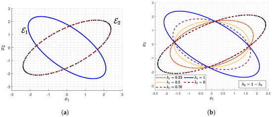
Figure 1. (a) For given ellipsoids ${\mathcal{E}}_1$ and ${\mathcal{E}}_2$, (b) ${\mathcal{E}}_{\mathbf{\lambda }}=\{x|x^T{P}_{\mathbf{\lambda }}x\le {\alpha }_{\mathbf{\lambda }},P_{\mathbf{\lambda }}={\sum }_{i=1}^2{\lambda }_i{P}_i,{\alpha }_{\mathbf{\lambda }}={\sum }_{i=1}^2{\lambda }_i{\alpha }_i\}$.

Table 1. Convex combinations (5) is different from the one used in [17,18]. Note that $R_i={[P_i/\alpha ]}^{-1}$.

	${\mathcal{E}}_{\mathit{i}}$	${\mathcal{E}}_{\mathit{\lambda }}$
[17,18]	$\{x|x^T{R}_i^{-1}x\le 1\}$	$\{x|x^T{({\sum }_{i=1}^m{\lambda }_i{R}_i)}^{-1}x\le 1\}\in$ convex hull
This paper	$\{x|x^T{P}_{i}x\le {\alpha }_i\}$	$\{x|x^T({\sum }_{i=1}^m{\lambda }_i{P}_i)x\le {\sum }_{i=1}^m{\lambda }_i{\alpha }_i\}\in$ union

Assumption 2.

For given $Q\ge 0$ and $R>0$, suppose that there exist m pairs of $({\mathcal{E}}_i,{\kappa }_i(·)),i=1,\dots ,m,$ satisfying A.1-A.3 of Lemma 1, and $P_L\in {\mathbb{R}}^{n\times n}$ such that

$$\begin{array}{c}\hfill f{(x,{\kappa }_i(x))}^T{P}_{L}f(x,{\kappa }_i(x))-x^T{P}_{L}x\le -\ell (x,{\kappa }_i(x)),\forall x\in {\mathcal{E}}_{i}i=1,\dots ,m,\end{array}$$

(7)

where $P_L$ is a symmetric and positive definite matrix and ${\mathcal{E}}_i=\{x|x^T{P}_{i}x\le {\alpha }_i\}$.

In the literature, there are several methods to find an invariant set and a terminal penalty cost such that the stability of the quasi-infinite horizon-based MPC (3) can be guaranteed, e.g., [5,25,26]. In these studies, $V(x)=x^{T}Px$ is shown as a local Lyapunov function in the set $\mathcal{E}=\{x|x^{T}Px\le \alpha \}$ under a stabilizing control law $\kappa (x)=Kx$, meaning that A1-A4 in Lemma 1 are satisfied. Thus, $V(x)$ and $\mathcal{E}$ can be used as the terminal penalty and the terminal region of a nonlinear MPC, respectively. However, Assumption 2 requires the existence of a common local Lyapunov function $V=x^T{P}_{L}x$ defined in all the sets ${\mathcal{E}}_1,\dots ,{\mathcal{E}}_m$ [27]. Suppose that ${\kappa }_i(x),{\mathcal{P}}_i,{\alpha }_i$ satisfying Lemma 1 are given in the first place, the common Lyapunov function can be found by choosing a positive definite matrix $P_L>P_i$ such that the following holds true

$$\begin{array}{c}\hfill \underset{x\in {\mathcal{E}}_i}{min}\left[x^T{P}_{L}x-f{(x,{\kappa }_i(x))}^T{P}_{L}f(x,{\kappa }_i(x))-\ell (x,{\kappa }_i(x))\right]\ge 0,\forall i\in [1,m].\end{array}$$

(8)

Note that (8) is equivalent with (7). A method based on the existing method [5,25,26] can also be employed to make Assumption 2 holds true. In fact, the following lemma can be obtained by extending the result in [26].

Lemma 3.

Suppose that Assumption 1 holds true, and that the following linearized system of (1) in the neighborhood of the origin is controllable

$$\begin{array}{c}\hfill x_{k+1}=A{x}_k+B{u}_k.\end{array}$$

(9)

Let $u_k=K{x}_k$ be a stabilizing feedback control law with feedback gain K and P be a positive definite matrix satisfying

$$\begin{array}{c}\hfill {\tau }^2{A}_{\mathsf{K}}^{T}P{A}_{\mathsf{K}}^T-P=-(Q+K^{T}RK),\end{array}$$

(10)

where $A_{\mathsf{K}}:=A+BK$, $\tau \in \left(1,\frac{1}{|{\lambda }_{max}(A_{\mathsf{K}})|}\right)$. Moreover, suppose that $P_L\in {\mathcal{R}}^{n\times n}$ is a positive definite matrix such that

$$\begin{array}{c}\hfill {\tau }^2{A}_{\mathsf{K}}^T{P}_L{A}_{\mathsf{K}}-P_L\le {\tau }^2{A}_{\mathsf{K}}^{T}P{A}_{\mathsf{K}}-P.\end{array}$$

(11)

Then, there exists a constant α specifying an ellipsoid in the form of $\mathcal{E}=\{x|x^{T}Px\le \alpha \}$ such that $K{x}_k\in \mathbb{U},\forall x\in \mathcal{E}$, $\mathcal{E}\in \mathbb{X}$, $\mathcal{E}$ is an invariant set for nonlinear system (1), and that the following holds true

$$\begin{array}{c}\hfill f{(x,Kx)}^T{P}_{L}f(x,Kx)-x^T{P}_{L}x\le -\ell (x,Kx),\forall x\in \mathcal{E}.\end{array}$$

(12)

Having this lemma, the sets ${\mathcal{E}}_1,\dots ,{\mathcal{E}}_m$ satisfying Assumption 2 can be obtained through the use of the linearized system and state feedback control laws. Specifically, $P_L$ is chosen such that (11) holds true for the given $(P_i,K_i)$, and ${\alpha }_i$ is chosen such that (12) holds true. The details of the method and the proof of the lemma are given in Appendix B.

Given ${\mathcal{E}}_1,\dots ,{\mathcal{E}}_m$, the proposed MPC with enlarged terminal region is computed by solving the following optimization problem

$$\begin{array}{}\mathrm{(13)}& \hfill \underset{{\mathcal{U}}_k,{\lambda }_{1,k},\dots ,{\lambda }_{m,k}}{min}& & J_N({\mathcal{U}}_k,x_k)\hfill \mathrm{}& \hfill \mathrm{subject\; to}\mathrm{}& \hfill & & x_{i+1|k}=f(x_{i|k},u_{i|k}),i\in \{0,\dots ,N-1\}\hfill \mathrm{}& \hfill & & u_{i|k}\in \mathbb{U},x_{i|k}\in \mathbb{X},i\in \{0,\dots ,N-1\}\hfill \mathrm{}& \hfill & & x_{0|k}=x_k,x_{N|k}\in {\mathcal{E}}_{\mathbf{\lambda },k}\hfill \mathrm{}& \hfill & & \sum _{i=1}^m{\lambda }_{i,k}=1,{\lambda }_{i,k}\ge 0,i\in \{1,\dots ,m\}\hfill \end{array}$$

where ${\mathcal{E}}_{\mathbf{\lambda },k}=\left\{x\in {\mathbb{R}}^n|x^T\left[{\sum }_{i=1}^m{\lambda }_{i,k}{P}_i\right]x\le {\sum }_{i=1}^m{\lambda }_{i,k}{\alpha }_i\right\}$,

$$\begin{array}{c}\hfill J_N({\mathcal{U}}_k,x_k)=\sum _{i=0}^{N-1}\ell (x_{i|k},u_{i|k})+x_{N|k}^T{P}_L{x}_{N|k},\end{array}$$

and ${\mathcal{U}}_k=\{u_{0|k},u_{1|k},\cdots ,u_{N-1|k}\}$. In the following, it is shown that the stability of the proposed MPC computed by (13) can be guaranteed.

Theorem 4.

For the nonlinear system (1), suppose that Assumptions 1 and 2 hold true, and that the optimization problem (13) with $Q\ge 0$ and $R>0$ is initially feasible. Then, the closed-loop system consisting of the system (1) and the nonlinear MPC obtained from (13) is asymptotically stable.

Proof. 

Let ${\lambda }_{1,k}^{*},\dots ,{\lambda }_{m,k}^{*}$, and $u_{i|k}^{*}$, $i=0,\dots N-1$, be the optimal solution of problem (13) at time k. Then, the optimal vector ${\mathcal{U}}_k^{*}$ and ${\mathcal{X}}_k^{*}$ are given by

$$\begin{array}{cc}\hfill {\mathcal{U}}_k^{*}& =\{u_{0|k}^{*},u_{1|k}^{*},\cdots ,u_{N-1|k}^{*}\},\hfill \\ \hfill {\mathcal{X}}_k^{*}& =\{x_{0|k}^{*},x_{1|k}^{*},\cdots ,x_{N-1|k}^{*},x_{N|k}^{*}\}.\hfill \end{array}$$

Having this, the optimal cost function at time k is given by

$$\begin{array}{c}\hfill J_N^{*}({{\mathcal{U}}^{*}}_k,x_k)=\sum _{i=0}^{N-1}\ell (x_{i|k}^{*},u_{i|k}^{*})+x_{N|k}^{*}{}^T{P}_L{x}_{N|k}^{*}.\end{array}$$

(14)

By Lemma 2, there is at least one j, $j\in \{1,\dots ,m\}$, such that $x_{N|k}^{*}\in {\mathcal{E}}_j$. Note that ${\lambda }_{j,k+1}=1$, ${\lambda }_{i,k+1}=0,i\in \{1,\dots ,m\},i\ne j$, are feasible at $k+1$ since ${\mathcal{E}}_j$ is an invariant set with ${\kappa }_j(x)$. Thus, the following is a feasible control sequence at $k+1$

$$\begin{array}{cc}\hfill {\tilde{\mathcal{U}}}_{k+1}& =\{u_{1|k}^{*},u_{2|k}^{*},\cdots ,u_{N-1|k}^{*},{\kappa }_j(x_{N|k}^{*})\}.\hfill \end{array}$$

(15)

The resulting state prediction is given by

$$\begin{array}{cc}\hfill {\tilde{\mathcal{X}}}_{k+1}& :=\{x_{1|k}^{*},x_{2|k}^{*},\cdots ,x_{N-1|k}^{*},x_{N|k}^{*},f(x_N^{*},{\kappa }_j(x_{N|k}^{*}))\}.\hfill \end{array}$$

(16)

where $f(x_N^{*},{\kappa }_j(x_{N|k}^{*}))\in {\mathcal{E}}_j$ due to the invariant set ${\mathcal{E}}_j$. Using (15) and (16), the cost function at $k+1$ is

$$\begin{array}{cc}\hfill J_N({\tilde{\mathcal{U}}}_{k+1},x_{k+1})& =\sum _{i=1}^{N-1}\ell (x_{i|k}^{*},u_{i|k}^{*})+\ell (x_{N|k}^{*},{\kappa }_j(x_{N|k}^{*}))+f{(x_N^{*},{\kappa }_j(x_{N|k}^{*}))}^T{P}_{L}f(x_N^{*},{\kappa }_j(x_{N|k}^{*})).\hfill \end{array}$$

(17)

Note that $J_N({\tilde{\mathcal{U}}}_{k+1},x_{k+1})$ is not the optimal cost function at $k+1$. Moreover, (17) can be rewritten as follows

$$\begin{array}{ccc}\hfill J_N({\tilde{\mathcal{U}}}_{k+1},x_{k+1})& =& J_N^{*}({{\mathcal{U}}^{*}}_k,x_k)-\ell (x_{0|k}^{*},u_{0|k}^{*})+\ell (x_{N|k}^{*},{\kappa }_j(x_{N|k}^{*}))\hfill \\ \hfill & & +f{(x_N^{*},{\kappa }_j(x_{N|k}^{*}))}^T{P}_{L}f(x_N^{*},{\kappa }_j(x_{N|k}^{*}))-x_{N|k}^{*}{}^T{P}_L{x}_{N|k}^{*},\hfill \end{array}$$

where $J_N^{*}({{\mathcal{U}}^{*}}_k,x_k)$ is defined in (14). Applying (7) to this inequality yields

$$\begin{array}{c}\hfill J_N({\tilde{\mathcal{U}}}_{k+1},x_{k+1})\le J_N^{*}({{\mathcal{U}}^{*}}_k,x_k)-\ell (x_{0|k}^{*},u_{0|k}^{*}).\end{array}$$

As a result, the optimal cost function at time $k+1$, denoted by $J_N^{*}({\mathcal{U}}_{k+1}^{*},x_{k+1})$, satisfies

$$\begin{array}{c}\hfill J_N^{*}({\mathcal{U}}_{k+1}^{*},x_{k+1})\le J_N({\tilde{\mathcal{U}}}_{k+1},x_{k+1})\le J_N^{*}({\mathcal{U}}_k^{*},x_k).\end{array}$$

In other words, the optimal cost function is a Lyapunov function for system (1). Having this and the terminal state constraint, nonlinear system (1) under the solution of (13) is asymptotically stable at the origin. □

Note that optimization problem (13) uses $x^T{P}_{L}x$ as the fixed penalty cost function but employs a time-varying terminal set ${\mathcal{E}}_{\mathbf{\lambda },k}=\left\{x\in {\mathbb{R}}^n|x^T\left[{\sum }_{i=1}^m{\lambda }_{i,k}{P}_i\right]x\le {\sum }_{i=1}^m{\lambda }_i{\alpha }_i\right\}$. Since ${\lambda }_{i,k},i=1,\dots ,m,$ can be any non-negative constants such that their sum is one, the union of ${\mathcal{E}}_1,\dots ,{\mathcal{E}}_m$ can be seen as the terminal set of (13), meaning that the proposed method potentially yields larger region of attraction when the region of attraction of each invariant set ${\mathcal{E}}_i$ is not the subset of the others, i.e., ${\mathcal{F}}_i^N\not\subset {\mathcal{F}}_j^N,i,j\in \{1,\dots ,m\},i\ne j$.

Although the resulting terminal set is not the convex hull of the predefined sets, the proposed method can be easily employed for a nonlinear system without the need for an LDI argument. Moreover, the ingredient sets ${\mathcal{E}}_i$ can be obtained using a similar procedure as in [5,25], or [26]. In the next section, numerical simulations are used to investigate the performance of the proposed MPC for a nonlinear system.

4. Example

In this section, the optimization problem (13) is employed for two nonlinear systems. At first, numerical simulation on a control-affine system with $x\in {\mathbb{R}}^2$ is presented. Then, a three-dimensional system is used to investigate the proposed method for a general nonlinear system.

4.1. A Two-Dimensional Nonlinear System

Consider the following nonlinear system

$$\begin{array}{ccc}\hfill {\dot{x}}_1& =& -20x_1+10x_2+6u+10x_1^{2}u,\hfill \\ \hfill {\dot{x}}_2& =& 20x_1-20x_2+6u-40x_2^{2}u,\hfill \end{array}$$

where $x_1,x_2\in \mathbb{R}$. The system is subjected to constraints $-0.1\le u\le 0.1$, $-2\le x_1\le 2$, and $-2\le x_2\le 2$. The system is discretized and linearized with sampling time $T=0.05$. For given $Q=diag([0.50.5])$ and $R=0.5$, suppose that a state feedback controller is used as a stabilizing control law, i.e., ${\kappa }_i(x)=K_{i}x$. Moreover, consider two pairs of $({\mathcal{E}}_i,{\kappa }_i(x))$, $i=1,2,$ and $P_L$ satisfying Assumption 2 given by

$$\begin{array}{ccc}\hfill K_1& =& \left[\begin{array}{cc}-0.0865& 0.1364\end{array}\right],K_2=\left[\begin{array}{cc}-0.1246& 0.1520\end{array}\right],\hfill \\ \hfill P_1& =& \left[\begin{array}{cc}9.2062& -5.7551\\ -5.7551& 5.4322\end{array}\right],P_2=\left[\begin{array}{cc}3.8403& 1.2193\\ 1.2193& 1.6077\end{array}\right],\hfill \\ \hfill P_L& =& \left[\begin{array}{cc}11.7274& -3.9370\\ -3.9370& 7.9271\end{array}\right],\hfill \end{array}$$

where ${\alpha }_1=0.95$, ${\alpha }_2=0.67$, and $P_L$ is computed using the procedure described in Appendix B. Figure 2 shows the sets ${\mathcal{E}}_i,i=1,2,$ and the estimate of region of attraction ${\mathcal{F}}_1^N$ and ${\mathcal{F}}_2^N$ for $N=2$. In this example, the resulting region of attraction from ${\mathcal{E}}_i$ is estimated by applying ${\mathcal{E}}_i$ as a fixed terminal set for different initial conditions. The proposed MPC results in a time-varying terminal set at each sampling time ${\mathcal{E}}_{\mathbf{\lambda }}={\lambda }_k{\mathcal{E}}_1+(1-{\lambda }_k){\mathcal{E}}_2$ where ${\lambda }_k\in \mathbb{R}$ is depicted in Figure 3. Figure 4 demonstrates that, for any $x_0\in {\mathcal{F}}_1^N\cup {\mathcal{F}}_2^N$, the states are steered to the origin. Moreover, the input constraint is satisfied as shown in Figure 5.

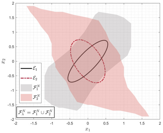
Figure 2. The invariant set ${\mathcal{E}}_i$ and an estimate of the corresponding region of attraction ${\mathcal{F}}_i^N$ with $N=2$. Since ${\mathcal{E}}_{\lambda }\in {\mathcal{E}}_1\cup {\mathcal{E}}_2$, a larger region of attraction can be obtained, i.e., ${\mathcal{F}}_{\mathbf{\lambda }}^N={\mathcal{F}}_1^N\cup {\mathcal{F}}_2^N$.

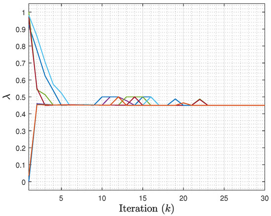
Figure 3. Variable $\lambda \in [0,1]$ defining the time-varying terminal set ${\mathcal{E}}_{\mathbf{\lambda }}$.

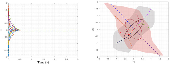
Figure 4. State $x=[x_1;x_2]$ converges to the origin for all $x_0\in {\mathcal{F}}_1^N\cup {\mathcal{F}}_2^N$.

Figure 5. Control input u satisfies input constraint.

As shown in Figure 2 and Table 2, some initial conditions lead to infeasibility when only one set (i.e., either ${\mathcal{E}}_1$ or ${\mathcal{E}}_2$) is considered for the terminal region. Meanwhile, thanks to the time-varying terminal set ${\mathcal{E}}_{\mathbf{\lambda }}$, ${\mathcal{F}}_1^N\cup {\mathcal{F}}_2^N$ is the resulting region of attraction. As a result, the proposed MPC is feasible for all six different initial states in Table 2, meaning that a larger region of attraction is obtained. Let ${\sum }_{t=0}^{\infty }{x}_t^{T}Q{x}_t+u_t^{T}R{u}_t$ be the simulation cost. It is shown in Table 2 and Figure 6 that, compared to the cost obtained by the MPC with ${\mathcal{E}}_i,i\in 1,2$ as the terminal region, the proposed MPC yields a comparable cost with a larger domain of attraction. In summary, the proposed nonlinear MPC with enlarged terminal set results in not only a larger region of attraction but also acceptable performance.

Table 2. Cost comparison between various terminal sets for given six different initial states.

${\mathit{x}}_0$	$[-1;-1]$	$[-0.1;-1.2]$	$[1.5;-1.9]$	$[1;1.5]$	$[0.1;1.2]$	$[-1.3;1.8]$
${\mathcal{E}}_1$	85.84	40.72	Infeasible	126.38	40.72	Infeasible
${\mathcal{E}}_2$	Infeasible	32.70	49.43	Infeasible	32.70	42.29
${\mathcal{E}}_{\mathbf{\lambda }}$	85.88	40.75	49.53	127.74	40.75	42.42

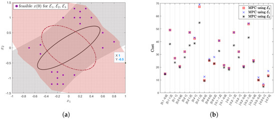
Figure 6. (a) Simulation cost ${\sum }_{t=0}^{\infty }{x}_t^{T}Q{x}_t+u_t^{T}R{u}_t$ is computed using 22 initial states which are feasible for ${\mathcal{E}}_i,i=1,2$. (b) The proposed MPC yields a similar cost with the one obtained using ${\mathcal{E}}_i,i\in \{1,2\}$.

4.2. A Three-Dimensional Nonlinear System

Consider the following nonlinear system [28,29]

$$\begin{array}{ccc}\hfill {\dot{x}}_1& =& -0.877x_1+x_3-0.088x_1{x}_3+0.47x_1^2-0.019x_2^2-x_1^2{x}_3+3.846x_1^3-0.215u_k+0.28x_1^{2}u+0.47x_1{u}^2+0.63u^3\hfill \\ \hfill {\dot{x}}_2& =& x_3\hfill \\ \hfill {\dot{x}}_3& =& -4.208x_1-0.396x_3-0.47x_1^2-3.564x_1^3-20.967u+6.265x_1^2{u}_k+46x_1{u}^2+61.1u^3.\hfill \end{array}$$

(18)

Note that the considered system is not linear in the input variable u. It is assumed that $\mathbb{U}=\{u|-3\le u\le 3\}$. Similar to the previous example, the weighting matrices Q and R are set to $Q=diag([0.50.50.5])$ and $R=0.5$. The following are two pairs of $({\mathcal{E}}_i,{\kappa }_i(x))$, $i=1,2,$ and $P_L$ satisfying Assumption 2

$$\begin{array}{ccc}\hfill K_1& =& \left[\begin{array}{ccc}-0.40& 1.57& 0.28\end{array}\right],K_2=\left[\begin{array}{ccc}-1.24& 1.95& 0.26\end{array}\right],\hfill \\ \hfill P_1& =& \left[\begin{array}{ccc}19.3& -70.5& -4.6\\ -70.5& 426.9& 29.9\\ -4.6& 29.9& 6.1\end{array}\right],P_2=\left[\begin{array}{ccc}136.1& -205.4& -11.1\\ -205.4& 341.4& 20.7\\ -11.1& 20.7& 3.7\end{array}\right],\hfill \\ \hfill P_L& =& \left[\begin{array}{ccc}832.3& -1221.2& -68.7\\ -1221.2& 2056.1& 122.8\\ -68.7& 122.8& 22.8\end{array}\right],\hfill \end{array}$$

and ${\alpha }_i=1$, $i=1,2$. The resulting feasible and invariant sets ${\mathcal{E}}_i,i=1,2,$ are shown in Figure 7. The set ${\mathcal{E}}_1$ is not a subset of ${\mathcal{E}}_2$, and vice versa. Figure 8 depicts several initial states when ${\mathcal{E}}_i,i\in 1,2$ is considered as the terminal set of a nonlinear MPC with $N=2$. Note that there are several initial states which are only feasible when ${\mathcal{E}}_1$ is employed as the terminal set of a nonlinear MPC. Likewise, there are several initial states which are only feasible when ${\mathcal{E}}_2$ is considered. In view of this, similar as in the previous example, using both ${\mathcal{E}}_1$ and ${\mathcal{E}}_2$ as the ingredient to define the time-varying terminal set ${\mathcal{E}}_{\mathbf{\lambda }}$ yields a larger region of attraction, i.e., ${\mathcal{E}}_{\mathbf{\lambda }}={\lambda }_k{\mathcal{E}}_1+(1-{\lambda }_k){\mathcal{E}}_2$. Applying the optimization problem (13) with $N=2$ to few different initial conditions of (18) results in ${\lambda }_k$ and the state trajectories $x(t)$ depicted in Figure 9a,b, respectively. Note that the resulting terminal set can be larger than the one obtained here if we consider more ingredient sets ${\mathcal{E}}_i$, i.e., $m>2$.

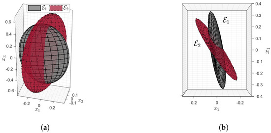
Figure 7. The invariant set ${\mathcal{E}}_1$ and ${\mathcal{E}}_2$, ${\mathcal{E}}_1,{\mathcal{E}}_2\in {\mathbb{R}}^3,i=1,2$, for system (18) where they are is plotted (a) in a three-dimensional space and (b) in view of $x_1$ and $x_2$ axes. Note that ${\mathcal{E}}_1\not\subset {\mathcal{E}}_2$ and ${\mathcal{E}}_2\not\subset {\mathcal{E}}_1$.

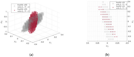
Figure 8. Few feasible initial states obtained using ${\mathcal{E}}_i,i=1,2$ as the terminal set of a nonlinear MPC with $N=2$, where they are is plotted (a) in a three-dimensional space and (b) in view of $x_1$ and $x_2$ axes. Note that some states are feasible only for the MPC with ${\mathcal{E}}_i$, $i\in \{1,2\}$.

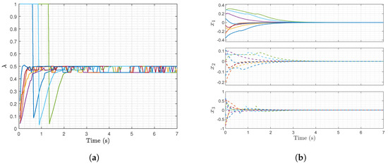
Figure 9. (a) Resulting $\lambda \in [0,1]$ defining the time-varying terminal set ${\mathcal{E}}_{\mathbf{\lambda }}\in {\mathbb{R}}^3$. (b) Trajectories from different initial states $x(0)$ which are feasible to either ${\mathcal{E}}_1$ or ${\mathcal{E}}_2$.

5. Conclusions

This paper proposes a new time-varying terminal set for the nonlinear MPC via a convex combination of given invariant and feasible sets. The resulting terminal set is the union of the predefined sets. Compared to the existing results on enlarging the terminal set through a convex combination strategy, the proposed approach appears to be more general since it does not require linear differential inclusion (LDI) representation of the nonlinear system in order to implement the proposed nonlinear MPC scheme. The existence of a common local Lyapunov function in all the ingredient invariant sets plays a key role in guaranteeing the stability of the proposed MPC. The paper gives a general way to use several sets obtained from different state-feedback gains. Possible future research includes the extension of this work to a tracking MPC problem.

Appendix B.1. Proof of Lemma 3

For all $\tau \in \left(1,\frac{1}{|{\lambda }_{max}(A_{\mathsf{K}})|}\right)$, all the eigenvalues of $\tau A_{\mathsf{K}}$ lie in the unit circle since $A_{\mathsf{K}}$ is Hurwitz. Thus, (10) admits a unique positive definite solution P. Since $(\mathbf{0},\mathbf{0})\in \mathbb{U}\times \mathbb{X}$, there exist $\gamma >0$ such that ${\mathcal{E}}_0=\{x|x^{T}Px\le \gamma \}$ where $Kx\in \mathbb{U},\forall x\in {\mathcal{E}}_0$, and ${\mathcal{E}}_0\subset \mathbb{X}$. In light of this, the dynamics (1) in $\mathcal{E}$ can be seen as an unconstrained nonlinear system, thereby, (1) with $u_k=K{x}_k$ can be written as

$$\begin{array}{c}\hfill x_{k+1}=A_{\mathsf{K}}{x}_k+\mathsf{\Phi }{x}_k,\end{array}$$

(A1)

where $\mathsf{\Phi }(x_k):=f(x_k,K{x}_k)-A_{\mathsf{K}}{x}_k$. Then, it remains to show that there exists $\alpha \in [0,\gamma )$ such that (12), i.e., invariance holds true. Consider a candidate Lyapunov function $V(x)=x^T{P}_{L}x$ for $P_L$ satisfying (11). It follows that

$$\begin{array}{ccc}\hfill V(x_{k+1})-V(x_k)& =& {\left(A_{\mathsf{K}}{x}_k+\mathsf{\Phi }(x_k)\right)}^T{P}_L(A_{\mathsf{K}}{x}_k+\mathsf{\Phi }(x_k))-x_k^T{P}_L{x}_k\hfill \\ & =& {\tau }^2{x}_k^T{A}_{\mathsf{K}}^T{P}_L{A}_{\mathsf{K}}{x}_k-x_k^T{P}_L{x}_k+(1-{\tau }^2)x_k^T{A}_{\mathsf{K}}^T{P}_L{A}_{\mathsf{K}}{x}_k\hfill \\ & & +2x_k^T{A}_{\mathsf{K}}^T{P}_L\mathsf{\Phi }(x_k)+{\mathsf{\Phi }}^T(x_k)P_L\mathsf{\Phi }(x_k).\hfill \end{array}$$

(A2)

In view of (11), there exists a positive semidefinite matrix $\mathsf{\Gamma }\in {\mathbb{R}}^{n\times n}$ such that

$$\begin{array}{c}\hfill {\tau }^2{A}_{\mathsf{K}}^T{P}_L{A}_{\mathsf{K}}-P_L={\tau }^2{A}_{\mathsf{K}}^{T}P{A}_{\mathsf{K}}-P-\mathsf{\Gamma }\end{array}$$

(A3)

holds true, i.e., $\mathsf{\Gamma }=P_L-P-{\tau }^2{A}_{\mathsf{K}}^T(P_L-P)A_{\mathsf{K}}$. Using (A3) and the definition of $\mathsf{\Gamma }$, (A2) can be written as

$$\begin{array}{ccc}\hfill V(x_{k+1})& -& V(x_k)={\tau }^2{x}_k^T{A}_{\mathsf{K}}^{T}P{A}_{\mathsf{K}}{x}_k-x_k^{T}P{x}_k-\psi (x_k),\hfill \end{array}$$

(A4)

where

$$\begin{array}{ccc}\hfill \psi (x_k)& =& x_k^T\mathsf{\Gamma }{x}_k+({\tau }^2-1)x_k^T{A}_{\mathsf{K}}^T{P}_L{A}_{\mathsf{K}}{x}_k-2x_k^T{A}_{\mathsf{K}}^T{P}_L\mathsf{\Phi }(x_k)-{\mathsf{\Phi }}^T(x_k)P_L\mathsf{\Phi }(x_k).\hfill \end{array}$$

(A5)

Note that $V(x_{k+1})-V(x_k)\le {\tau }^2{x}_k^T{A}_{\mathsf{K}}^{T}P{A}_{\mathsf{K}}{x}_k-x_k^{T}P{x}_k$ when $\psi (x_k)\ge 0$. Recall that, according to the Taylor’s Theorem, for a continuous and twice differentiable function g on an open interval I around a, there is a value $\eta$ between a and b so that

$$\begin{array}{c}\hfill g(b)=g(a)+g^{\prime }(a)(b-a)+\frac{1}{2}g{}^{\prime \prime }(\eta ){(b-a)}^2.\end{array}$$

(A6)

In order to apply this to function $\mathsf{\Phi }$, let ${\eta }_k$ be some value between $a=\mathbf{0}$ and $b=x_k$. Then, function $\mathsf{\Phi }$ yields

$$\begin{array}{c}\hfill \mathsf{\Phi }(x_k)=\frac{1}{2}{x}_k^T\frac{{\partial }^{2}f({\eta }_k,K{\eta }_k)}{{\partial }^2{x}_k}{x}_k+\frac{1}{2}{x}_k^T\frac{{\partial }^{2}f({\eta }_k,K{\eta }_k)}{\partial x_k\partial u_k}K{x}_k+\frac{1}{2}{x}_k^T{K}^T\frac{{\partial }^{2}f({\eta }_k,K{\eta }_k)}{\partial u_k\partial x_k}{x}_k+\frac{1}{2}{x}_k^T{K}^T\frac{{\partial }^{2}f({\eta }_k,K{\eta }_k)}{{\partial }^2{u}_k}K{x}_k,\end{array}$$

owing to $\mathsf{\Phi }(a)=\mathsf{\Phi }(\mathbf{0})=0$ and ${\mathsf{\Phi }}^{\prime }(a)={\mathsf{\Phi }}^{\prime }(\mathbf{0})=0$. Denote

$$\begin{array}{c}\hfill C(\mathsf{\Phi }(x_k))=\frac{{\partial }^{2}f({\eta }_k,K{\eta }_k)}{{\partial }^2{x}_k}+\frac{{\partial }^{2}f({\eta }_k,K{\eta }_k)}{\partial x_k\partial u_k}K+K^T\frac{{\partial }^{2}f({\eta }_k,K{\eta }_k)}{\partial u_k\partial x_k}+K^T\frac{{\partial }^{2}f({\eta }_k,K{\eta }_k)}{{\partial }^2{u}_k}K.\end{array}$$

Let $C_M$ be defined as follows

$$\begin{array}{c}\hfill C_M:=\underset{{\eta }_k\in {\mathcal{E}}_0}{sup}\parallel C({\eta }_k)\parallel .\end{array}$$

Thus, $\parallel \mathsf{\Phi }(x_k)\parallel \le \frac{1}{2}{C}_M{\parallel x_k\parallel }^2$ for all $x_k\in {\mathcal{E}}_0$. Furthermore,

$$\begin{array}{ccc}\hfill 2x_k^T{A}_{\mathsf{K}}^T{P}_L\mathsf{\Phi }(x_k)+{\mathsf{\Phi }}^T(x_k)P_L\mathsf{\Phi }(x_k)& \le & C_M\parallel A_{\mathsf{K}}\parallel \parallel P_L\parallel \parallel x_k{\parallel }^3+\frac{C_M^2}{4}\parallel P_L\parallel \parallel x_k{\parallel }^4.\hfill \end{array}$$

(A7)

Let $\alpha \in [0,\gamma )$ such that

$$\begin{array}{c}\hfill C_M\parallel A_{\mathsf{K}}\parallel \parallel P_L\parallel \parallel x_k\parallel +\frac{C_M^2}{4}\parallel P_L\parallel \parallel x_k{\parallel }^2\le ({\tau }^2-1){\lambda }_{min}(A_{\mathsf{K}}^T{P}_L{A}_{\mathsf{K}})+{\lambda }_{min}(\mathsf{\Gamma }),\end{array}$$

for all $x_k\in \mathcal{E}$. Then, $C_M\parallel A_{\mathsf{K}}\parallel \parallel P_L\parallel \parallel x_k{\parallel }^3+\frac{C_M^2}{4}\parallel P_L\parallel \parallel x_k{\parallel }^4\le ({\tau }^2-1){\lambda }_{min}(A_{\mathsf{K}}^T{P}_L{A}_{\mathsf{K}})\parallel x_k{\parallel }^2+{\lambda }_{min}(\mathsf{\Gamma }){\parallel x_k\parallel }^2$. Note that ${\lambda }_{min}(A_{\mathsf{K}}^T{P}_L{A}_{\mathsf{K}}){\parallel x_k\parallel }^2\le x_k^T{A}_{\mathsf{K}}^T{P}_L{A}_{\mathsf{K}}{x}_k$ and ${\lambda }_{min}(\mathsf{\Gamma }){\parallel x_k\parallel }^2\le x_k^T\mathsf{\Gamma }{x}_k$. With this and (A7) in mind,

$$\begin{array}{ccc}\hfill 2x_k^T{A}_{\mathsf{K}}^T{P}_L\mathsf{\Phi }(x_k)+{\mathsf{\Phi }}^T(x_k)P_L\mathsf{\Phi }(x_k)& \le & ({\tau }^2-1)x_k^T{A}_{\mathsf{K}}^T{P}_L{A}_{\mathsf{K}}{x}_k+x_k^T\mathsf{\Gamma }{x}_k,\forall x_k\in \mathcal{E}.\hfill \end{array}$$

It follows that $\psi (x_k)\ge 0$ for all $x_k\in \mathcal{E}$. Substituting this to (A4) and using (10) yield $V(x_{k+1})-V(x_k)\le -x_k^{T}Q{x}_k-x_k^T{K}^{T}RK{x}_k$.

Appendix B.2. A Common Lyapunov Function

In view of the proof above, for given $(K_i,P_i)$ satisfying (10), the sets ${\mathcal{E}}_1,\dots ,{\mathcal{E}}_m$ described in Assumption 2 can be found by reducing ${\alpha }_i\in [0,{\gamma }_i)$ such that the following holds true

$$\begin{array}{c}\hfill \underset{x\in {\mathcal{E}}_i}{min}{\psi }_i(x)\ge 0,\forall i\in [1,m],\end{array}$$

(A8)

where, according to (A5),

$$\begin{array}{ccc}\hfill {\psi }_i(x)& =& x^T{\mathsf{\Gamma }}_{i}x+({\tau }_i^2-1)x^T{A}_{\mathsf{K},i}^T{P}_L{A}_{\mathsf{K},i}x-2x^T{A}_{\mathsf{K},i}^T{P}_L{\mathsf{\Phi }}_i(x)-{\mathsf{\Phi }}_i^T(x)P_L{\mathsf{\Phi }}_i(x),\hfill \end{array}$$

and $P_L$ satisfying ${\tau }_i^2{A}_{\mathsf{K},i}^T{P}_L{A}_{\mathsf{K},i}-P_L\le {\tau }_i^2{A}_{\mathsf{K},i}^T{P}_i{A}_{\mathsf{K},i}-P_i$ for all $i\in [1,m]$. Note that nonlinear optimization (A8) is similar to the optimization used in [5,25,26].

References

- Mayne, D.Q.; Rawlings, J.B.; Rao, C.V.; Scokaert, P.O.M. Constrained model predictive control: Stability and optimality. Automatica 2000, 36, 789–814. [Google Scholar] [CrossRef]
- Rossiter, J.A. Model-Based Predictive Control: A Practical Approach; CRC Press: Boca Raton, FL, USA, 2013. [Google Scholar]
- Lee, J.W.; Kwon, W.H.; Choi, J. On Stability of Constrained Receding Horizon Control with Finite Terminal Weighting Matrix. Automatica 1998, 34, 1607–1612. [Google Scholar] [CrossRef]
- Mayne, D.Q.; Michalska, H. Receding horizon control of nonlinear systems. IEEE Trans. Autom. Control. 1990, 35, 814–824. [Google Scholar] [CrossRef]
- Chen, H.; AllGöwer, F. A Quasi-Infinite Horizon Nonlinear Model Predictive Control Scheme with Guaranteed Stability. Automatica 1998, 34, 1205–1217. [Google Scholar] [CrossRef]
- Yu, S.; Reble, M.; Chen, H.; Allgöwer, F. Inherent robustness properties of quasi-infinite horizon nonlinear model predictive control. Automatica 2014, 50, 2269–2280. [Google Scholar] [CrossRef]
- Magni, L.; Nicolao, G.; Magnani, L.; Scattolini, R. A stabilizing model-based predictive control algorithm for nonlinear systems. Automatica 2001, 37, 1351–1362. [Google Scholar] [CrossRef]
- De Doná, J.; Seron, M.; Mayne, D.; Goodwin, G. Enlarged terminal sets guaranteeing stability of receding horizon control. Syst. Control. Lett. 2002, 47, 57–63. [Google Scholar] [CrossRef]
- Limon, D.; Alamo, T.; Camacho, E. Enlarging the domain of attraction of MPC controllers. Automatica 2005, 41, 629–635. [Google Scholar] [CrossRef]
- González, A.H.; Odloak, D. Enlarging the domain of attraction of stable MPC controllers, maintaining the output performance. Automatica 2009, 45, 1080–1085. [Google Scholar] [CrossRef]
- Chen, W.H.; O’Reilly, J.; Ballance, D.J. On the terminal region of model predictive control for non-linear systems with input/state constraints. Int. J. Adapt. Control. Signal Process. 2003, 17, 195–207. [Google Scholar] [CrossRef]
- Bacic, M.; Cannon, M.; Kouvaritakis, B. General interpolation for input-affine nonlinear systems. In Proceedings of the 2004 American Control Conference, Boston, MA, USA, 30 June–2 July 2004; Volume 3, pp. 2010–2014. [Google Scholar]
- Zhao, M.; Jiang, C.; Tang, X.; She, M. Interpolation Model Predictive Control of Nonlinear Systems Described by Quasi-LPV Model. Autom. Control. Comput. Sci. 2018, 52, 354–364. [Google Scholar] [CrossRef]
- Yu, S.; Chen, H.; Böhm, C.; Allgöwer, F. Enlarging the terminal region of NMPC with parameter-dependent control law. In Nonlinear Model Predictive Control-Towards New Challenging Applications; Magni, L., Raimondo, D., Allgöwer, F., Eds.; Lecture Notes in Control and Information Sciences; Springer: Berlin/Heidelberg, Germany, 2009; pp. 69–78. [Google Scholar]
- Bacic, M.; Cannon, M.; Lee, Y.I.; Kouvaritakis, B. General interpolation in MPC and its advantages. IEEE Trans. Autom. Control. 2003, 48, 1092–1096. [Google Scholar] [CrossRef]
- Rossiter, J.A.; Kouvaritakis, B.; Bacic, M. Interpolation based computationally efficient predictive control. Int. J. Control. 2004, 77, 290–301. [Google Scholar] [CrossRef]
- Pluymers, B.; Roobrouck, L.; Buijs, J.; Suykens, J.; Moor, B.D. Constrained linear MPC with time-varying terminal cost using convex combinations. Automatica 2005, 41, 831–837. [Google Scholar] [CrossRef]
- Kim, J.S.; Lee, Y.I. An Interpolation Technique for Input Constrained Robust Stabilization. Int. J. Control. Autom. Syst. 2018, 16, 1569–1576. [Google Scholar] [CrossRef]
- Kothare, M.V.; Balakrishnan, V.; Morari, M. Robust constrained model predictive control using linear matrix inequalities. Automatica 1996, 32, 1361–1379. [Google Scholar] [CrossRef]
- Shang, Y. Couple-group consensus of continuous-time multi-agent systems under Markovian switching topologies. J. Frankl. Inst. 2015, 352, 4826–4844. [Google Scholar] [CrossRef]
- Shang, Y. Consensus seeking over Markovian switching networks with time-varying delays and uncertain topologies. Appl. Math. Comput. 2016, 273, 1234–1245. [Google Scholar] [CrossRef]
- Bohm, C.; Raff, T.; Findeisen, R.; Allgower, F. Calculating the terminal region of NMPC for Lure systems via LMIs. In Proceedings of the 2008 the American Control Conference, Seattle, WA, USA, 11–13 June 2008. [Google Scholar]
- Rawlings, J.B.; Mayne, D.Q. Model Predictive Control: Theory and Design; Nob Hill Pub.: Madison, WI, USA, 2009. [Google Scholar]
- Schröcker, H.P. Uniqueness results for minimal enclosing ellipsoids. Comput. Aided Geom. Des. 2008, 25, 756–762. [Google Scholar] [CrossRef]
- Johansen, T.A. Approximate explicit receding horizon control of constrained nonlinear systems. Automatica 2004, 40, 293–300. [Google Scholar] [CrossRef]
- Yu, S.; Qu, T.; Xu, F.; Chen, H.; Hu, Y. Stability of finite horizon model predictive control with incremental input constraints. Automatica 2017, 79, 265–272. [Google Scholar] [CrossRef]
- Liberzon, D. Switching in Systems and Control; Birkhäuser: Boston, MA, USA, 2003. [Google Scholar]
- Garrard, W.L.; Jordan, J.M. Design of nonlinear automatic flight control systems. Automatica 1977, 13, 497–505. [Google Scholar] [CrossRef]
- Kaiser, E.; Kutz, J.N.; Brunton, S.L. Sparse identification of nonlinear dynamics for model predictive control in the low-data limit. Proc. R. Soc. Math. Phys. Eng. Sci. 2018, 474. [Google Scholar] [CrossRef] [PubMed]
Publisher’s Note: MDPI stays neutral with regard to jurisdictional claims in published maps and institutional affiliations. |
© 2020 by the authors. Licensee MDPI, Basel, Switzerland. This article is an open access article distributed under the terms and conditions of the Creative Commons Attribution (CC BY) license (http://creativecommons.org/licenses/by/4.0/).