On First-Passage Times and Sojourn Times in Finite QBD Processes and Their Applications in Epidemics

Abstract

In this paper, we revisit level-dependent quasi-birth-death processes with finitely many possible values of the level and phase variables by complementing the work of Gaver, Jacobs, and Latouche (Adv. Appl. Probab. 1984), where the emphasis is upon obtaining numerical methods for evaluating stationary probabilities and moments of first-passage times to higher and lower levels. We provide a matrix-analytic scheme for numerically computing hitting probabilities, the number of upcrossings, sojourn time analysis, and the random area under the level trajectory. Our algorithmic solution is inspired from Gaussian elimination, which is applicable in all our descriptors since the underlying rate matrices have a block-structured form. Using the results obtained, numerical examples are given in the context of varicella-zoster virus infections.

1. Introduction

In this paper, we shall be concerned with time-homogeneous continuous-time Markov chains $\mathcal{X}=\left\{\right(I\left(t\right),J\left(t\right)):t\in [0,\infty \left)\right\}$ that take values in a bivariate state space $\mathcal{S}=\left\{\right(i,j):i\in \{0,\dots ,N\},$$j\in \{0,\dots ,M_i\}\}$, for integers $M_i\in {\mathbb{N}}_0$ with $i\in \{0,\dots ,N\}$ and $N\in \mathbb{N}$, and have an irreducible infinitesimal generator $\mathbf{Q}$ with block-tridiagonal representation

$$\begin{array}{ccc}\hfill \mathbf{Q}& =& \left(\begin{array}{ccccc}{\mathbf{Q}}_{0,0}& {\mathbf{Q}}_{0,1}& & & \\ {\mathbf{Q}}_{1,0}& {\mathbf{Q}}_{1,1}& {\mathbf{Q}}_{1,2}& & \\ & \ddots & \ddots & \ddots & \\ & & {\mathbf{Q}}_{N-1,N-2}& {\mathbf{Q}}_{N-1,N-1}& {\mathbf{Q}}_{N-1,N}\\ & & & {\mathbf{Q}}_{N,N-1}& {\mathbf{Q}}_{N,N}\end{array}\right),\hfill \end{array}$$

(1)

where the sub-matrices ${\mathbf{Q}}_{i,i^{\prime }}$ are of dimension $(1+M_i)\times (1+M_{i^{\prime }})$, for $i^{\prime }\in \{max\{0,i-1\},i,min\{i+1,N\}\}$, i.e., from any state $(i,j)$, process $\mathcal{X}$ can access only states $(i^{\prime },k)$ with $|i^{\prime }-i|\le 1$ and $k\in M_{i^{\prime }}$, whence $I\left(t\right)$ can change its value by $\{-1,0,1\}$ only. These Markov chains are referred to as finite quasi-birth-death (QBD) processes, being its first variable $I\left(t\right)$ called the level, and the second one $J\left(t\right)$ the phase; see e.g. Gaver et al. [1]. They are capable of modeling, in a unified and algorithmically tractable manner, relevant systems, such as queueing models (Baumann and Sandmann [2]; Gun and Makowski [3]; Perel and Yechiali [4]; Ye and Li [5]), communication networks (Artalejo and Gómez-Corral [6]; Artalejo and Lopez-Herrero [7]), reliability and manufacturing systems (Chakravarthy and Gómez-Corral [8]; Moghaddass et al. [9]), and epidemic models (Amador and Gómez-Corral [10]; Artalejo et al. [11]; Economou et al. [12]; Gamboa and Lopez-Herrero [13]), among others.

The properties of finite QBD processes have been studied extensively in continuous and discrete time. For a comprehensive discussion, see, e.g., the monograph of Latouche and Ramaswami (Chapter 10 in Reference [14]) and references therein. Most of the theoretical work so far carried out in this setting is concerned with the stationary probability vector. More concretely, Hajek [15] observes that, under certain conditions for the underlying transition matrices, the stationary vector of a finite level-independent QBD process has a mixed matrix-geometric form; for a related numerical method that exploits invariant subspace computations, see the paper by Akar et al. [16]. Gaver et al. (Section 2 in Reference [1]) use linear level reduction, which is a refined probabilistic justification for block-Gaussian elimination (Latouche and Ramaswami (Remark 10.1.6 in Reference [14]); Stewart [17]). Ye and Li [5] (see also Latouche and Ramaswami (Section 10.2 in Reference [14])) propose an efficient computational approach, termed folding algorithm, which is seen to be a form of odd-even reduction, and Naoumov [18] presents an algebraically matrix-multiplicative approach for a finite QBD process. $LU$-type and $UL$-type $RG$-factorizations are used by Li and Cao (Section 3.1 in Reference [19]) in an attempt to clarify the relations among those results in Gaver et al. [1], Hajek [15], and Naoumov [18]. Elhafsi and Molle [20] present a matrix-geometric expression for the stationary vector of a finite level-independent QBD process in terms of a set of rate matrices and compare their solution with several existing solution methods, including the approaches of de Nitto Persone and Grassi [21], Gun and Makowski [3], and Hajek [15], and a more general solution of Le Boudec [22] for upper block Hessenberg matrices. Other approaches are related to the group inverse (da Silva Soares and Latouche [23]) and the matrix continued fraction algorithm (Baumann and Sandmann [24]).

Despite their simplicity and their success in stochastic modeling, there have been few contributions dealing with random descriptors different from the stationary probability vector in the theory of finite QBD processes. Gaver et al. (Sections 3–4 in Reference [1]) use Laplace-Stieltjes transforms of first-passage times from level $l(i-1)$ to level $l\left(i\right)$, where the $i^{\prime }$th level is defined as $l\left(i^{\prime }\right)=\{(i^{\prime },j):j\in \{0,\dots ,M_{i^{\prime }}\left\}\right\}$, to derive a product-form expression for the Laplace-Stieltjes transform of the first-passage time from level $l(i-1)$ to higher levels $l\left(i^{\prime }\right)$, with $i^{\prime }\in \{i,\dots ,N\}$, and similar results for the first-passage times to lower levels. An up-integral functional is defined in the paper by Li and Cao [19,] (Section 4) and explicit expressions for the Laplace transforms of its conditional distributions and moments are written in terms of the underlying R- and G-measures. Li and Sheng [25] propose and implement a generalized folding algorithm for transient analysis of a finite QBD process, which entails the solution of $\mathbf{x}\mathbf{Q}=\mathbf{a}$, where $\mathbf{a}$ is a predetermined boundary condition vector, and present comprehensive numerical examples on transient queueing behavior with correlated arrivals. Based on the R- and G-measures, Shin [26] derives an algorithm for computing the fundamental matrix of a finite QBD process with absorbing states and shows how the resulting algorithm can be applied to absorption probabilities, sojourn time distributions, the busy period and the stationary vector in the multiprogramming model discussed by Neuts [27] (pp. 245–253) and the $M/M/c$ retrial queue with finite orbit capacity (Artalejo and Gómez-Corral (Chapter 4 in Reference [28])). Recently, Gómez-Corral and López-García [29] use matrix calculus and exploit the specific structure of the infinitesimal generator $\mathbf{Q}$ in (1) to provide the sensitivities and the elasticities of finite QBD processes with respect to model parameters, with special emphasis on first-passage times to level $l\left(0\right)$ and hitting probabilities, the maximum level visited by the process before reaching states in level $l\left(0\right)$ and the stationary vector, and illustrate the approach by means of applying multi-type versions of the susceptible-infective (SI) and susceptible-infective-susceptible (SIS) epidemic models to the spread of antibiotic-sensitive and antibiotic-resistant bacterial strains in a hospital ward.

The objective of this paper was to complement the work of Gaver et al. [1] by showing here that, in the spirit of algorithmic probability, the fundamental ideas of Gaver et al. [1] extend beyond the stationary distribution and first-passage times to higher and lower levels, and apply to more complex descriptors arising from epidemic models. The methods we shall follow in this paper are suggested by some related work of Amador et al. [30], Baumann and Sandmann [31], Lefèvre and Simon [32], and Neuts [33], where, for instance, the random length of an outbreak and the final size of the epidemic in SIR-type and SIS-type epidemic models correspond to the absorption time and the hitting probabilities in a suitably defined absorbing QBD process, and related block-structured Markov processes. In order to simplify the presentation throughout the paper, we shall assume that $(1,j)$ is the initial state of process $\mathcal{X}$, for phases $j\in \{0,\dots ,M_1\}$, which is related to an invasion time in the spread of a disease.

The paper is organized as follows. In Section 2, we derive recursive expressions for the hitting probabilities of restricted versions of process $\mathcal{X}$. In Section 3, we characterize the probability laws of the number of upcrossings from level $l(K-1)$ to states in $l\left(K\right)$, for a predetermined threshold $K\in \{2,\dots ,N\}$, and the total time spent at states in higher levels before reaching states in level $l\left(0\right)$. In Section 4, we study the random area under the trajectory of the integer-valued random variable $I\left(t\right)$ before process $\mathcal{X}$ visits states in $l\left(0\right)$ for the first time. Numerical examples are given in Section 5 in the setting of varicella-zoster virus infections, and concluding remarks follow in Section 6.

2. First-Passage Times to Higher Levels and Restricted Hitting Probabilities

Let us consider the first-passage time ${\eta }_{(1,j),K}$ to level $l\left(K\right)$ from state $(1,j)$, for a predetermined integer $K\in \{2,\dots ,N\}$, and the first-passage time ${\overline{\eta }}_{(1,j),0}$ to level $l\left(0\right)$ from state $(1,j)$, with $j\in \{0,\dots ,M_1\}$. For phases $n\in \{0,\dots ,M_K\}$, we let $P_{(1,j),K}\left(n\right)$ denote the restricted hitting probability

$$\begin{array}{c}\hfill P\left((I\left({\eta }_{(1,j),K}\right),J\left({\eta }_{(1,j),K}\right))=(K,n),{\eta }_{(1,j),K}<{\overline{\eta }}_{(1,j),0}|(I\left(0\right),J\left(0\right))=(1,j)\right),\end{array}$$

which is related to the dynamics of process $\mathcal{X}$ evolving on those sample paths satisfying ${\eta }_{(1,j),K}<{\overline{\eta }}_{(1,j),0}$.

Remark 1.

Note that the probability law of ${\eta }_{(1,j),K}$ (respectively, ${\overline{\eta }}_{(1,j),0}$) corresponds to the conditional distribution of the random variable ${\tau }_{n,m}$ defined in Section 3 of Reference [1] with $n=2$ and $m=K$ (respectively, ${\overline{\tau }}_{m,n}$ defined in Section 4 of Reference [1] with $m=n=0$), given that $\left(I\right(0),J(0\left)\right)=(1,j)$. A product-form expression for the Laplace-Stieltjes transform of ${\eta }_{(1,j),K}$ and recursive relations for its expectation (respectively, the expectation of ${\overline{\eta }}_{(1,j),0}$) can be then obtained from Equations (3.9) and (3.12)–(3.14) (respectively, (4.4)–(4.6)) of Reference [1].

In order to derive expressions for the restricted hitting probabilities $\{P_{(1,j),K}\left(n\right):n\in \{0,\dots ,M_K\}\}$, it is useful to consider an auxiliary absorbing process $\mathcal{X}\left(K\right)=\left\{X\right(t):t\ge 0\}$ that takes values in the state space $\mathcal{S}\left(K\right)=\left\{0\right\}\cup {\bigcup }_{i=1}^{K-1}l\left(i\right)\cup \left\{K\right\}$, where 0 and K are assumed to be absorbing states and ${\bigcup }_{i=1}^{K-1}l\left(i\right)$ is a class of transient states. The infinitesimal generator of $\mathcal{X}\left(K\right)$ has the block-structured form

$$\begin{array}{ccc}\hfill \mathbf{Q}\left(K\right)& =& \left(\begin{array}{ccc}0& {\mathbf{0}}_{K-1+{\sum }_{i=1}^{K-1}{M}_i}^T& 0\\ {\mathbf{t}}_0\left(K\right)& \mathbf{T}\left(K\right)& {\mathbf{t}}_K\left(K\right)\\ 0& {\mathbf{0}}_{K-1+{\sum }_{i=1}^{K-1}{M}_i}^T& 0\end{array}\right),\hfill \end{array}$$

(2)

where the column vector ${\mathbf{0}}_a$ is the null vector of order a, ${}^T$ denotes transposition, the sub-matrix $\mathbf{T}\left(K\right)$ is obtained from $\mathbf{Q}$ by removing rows and columns associated with states in $l\left(0\right)$ and ${\bigcup }_{i=K}^{N}l\left(i\right)$, the column vectors ${\mathbf{t}}_0\left(K\right)$ and ${\mathbf{t}}_K\left(K\right)$ have the form

$$\begin{array}{ccc}\hfill {\mathbf{t}}_0\left(K\right)& =& \left(\begin{array}{c}{\mathbf{Q}}_{1,0}{\mathbf{1}}_{1+M_0}\\ {\mathbf{0}}_{K-2+{\sum }_{i=2}^{K-1}{M}_i}\end{array}\right),\mathrm{and}{\mathbf{t}}_K\left(K\right)=\left(\begin{array}{c}{\mathbf{0}}_{K-2+{\sum }_{i=1}^{K-2}{M}_i}\\ {\mathbf{Q}}_{K-1,K}{\mathbf{1}}_{1+M_K}\end{array}\right),\hfill \end{array}$$

and the column vector ${\mathbf{1}}_a$ is the unit vector of order a. It is clear that, starting from states in ${\bigcup }_{i=1}^{K-1}l\left(i\right)$, the process $\mathcal{X}\left(K\right)$ defined by (2) is the restriction of process $\mathcal{X}$ to the states in ${\bigcup }_{i=1}^{K-1}l\left(i\right)$ before the first entrance into states in $l\left(0\right)\cup {\bigcup }_{i=K}^{N}l\left(i\right)$. In particular, it is found that

$$\begin{array}{ccc}\hfill P({\eta }_{(1,j),K}<{\overline{\eta }}_{(1,j),0})& =& {\mathbf{e}}_{K-1+{\sum }_{i=1}^{K-1}{M}_i}(1+j)\left(-{\mathbf{T}}^{-1}\left(K\right)\right){\mathbf{t}}_K\left(K\right),\hfill \end{array}$$

(3)

where ${\mathbf{e}}_a\left(b\right)$ is a row vector of order a, in which entries are all equal to 0, except the bth entry which equals 1. The proof of (3) is based on the fact that the transition function $P\left(X\right(t)=K|X\left(0\right)=(1,j))$ of process $\mathcal{X}\left(K\right)$ is given by

$$\begin{array}{c}\hfill {\mathbf{e}}_{K-1+{\sum }_{i=1}^{K-1}{M}_i}(1+j)\left({\mathbf{I}}_{K-1+{\sum }_{i=1}^{K-1}{M}_i}-exp\left\{\mathbf{T}\left(K\right)t\right\}\right)\left(-{\mathbf{T}}^{-1}\left(K\right)\right){\mathbf{t}}_K\left(K\right),\end{array}$$

which yields $P({\eta }_{(1,j),K}<{\overline{\eta }}_{(1,j),0})$ by taking the limit as $t\to \infty$, since the sub-matrix $\mathbf{T}\left(K\right)$ is stable and the real parts of its eigenvalues are all strictly negative.

By appealing to statement (b) of Lemma 1 in the paper by Gaver et al. [1], it is noted that the matrix $-{\mathbf{T}}^{-1}\left(K\right)$ records expected total times that process $\mathcal{X}$ spends at states in ${\bigcup }_{i=1}^{K-1}l\left(i\right)$ before $\mathcal{X}$ visits states in either $l\left(0\right)$ or $l\left(K\right)$ for the first time, provided that $\mathcal{X}$ starts from any initial state in ${\bigcup }_{i=1}^{K-1}l\left(i\right)$. Furthermore, a slight modification of statement (c) of Lemma 1 in Reference [1] permits to establish that, by denoting by ${\mathbf{T}}_K\left(K\right)$ the matrix recording infinitesimal rates associated with transitions to states in $l\left(K\right)$ from ${\bigcup }_{i=1}^{K-1}l\left(i\right)$, the matrix $-{\mathbf{T}}^{-1}\left(K\right){\mathbf{T}}_K\left(K\right)$ consists of first passage probabilities to level $l\left(K\right)$, given that $\mathcal{X}$ starts from any state in ${\bigcup }_{i=1}^{K-1}l\left(i\right)$.

This means that the $(1+j)$th row of $-{\mathbf{T}}^{-1}\left(K\right){\mathbf{T}}_K\left(K\right)$ consists of the restricted hitting probabilities $P_{(1,j),K}\left(n\right)$, for phases $n\in \{0,\dots ,M_K\}$, and consequently, recursive relations for these probabilities can be derived from Theorem 4.2.4 of the book by Hunter [34] by observing that $\mathbf{T}\left(K\right)$ can be written in terms of the sub-matrix $\mathbf{T}(K-1)$.

Theorem 1.

For a predetermined integer $K\in \{2,\dots ,N\}$ and an initial state $(1,j)$ with $j\in \{0,\dots ,M_1\}$, the restricted hitting probability $P_{(1,j),K}\left(n\right)$ is specified by

$$\begin{array}{ccc}\hfill P_{(1,j),K}\left(n\right)& =& \mathbf{u}(j,K){\mathbf{Q}}_{K-1,K}{\mathbf{e}}_{1+M_K}^T(1+n),\hfill \end{array}$$

(4)

for phases $n\in \{0,\dots ,M_K\}$, where

$$\begin{array}{ccc}\hfill \mathbf{u}(j,K)& =& \left\{\begin{array}{cc}{\mathbf{e}}_{1+M_1}(1+j)\left(-{\mathbf{Q}}_{1,1}^{-1}\right),\hfill & ifK=2,\hfill \\ {\mathbf{e}}_{K-2+{\sum }_{i=1}^{K-2}{M}_i}(1+j){\mathbf{V}}_{1,2}\left(K\right),\hfill & ifK\in \{3,\dots ,N\}.\hfill \end{array}\right.\hfill \end{array}$$

Moreover, the sub-matrices ${\mathbf{V}}_{1,2}\left(K\right)$, for integers $K\in \{3,\dots ,N\}$, are given by ${\mathbf{V}}_{1,2}\left(K\right)=-{\mathbf{T}}^{-1}(K-1){\mathbf{U}}_{1,2}\left(K\right){\mathbf{V}}_{2,2}\left(K\right)$, where

$$\begin{array}{ccc}\hfill {\mathbf{V}}_{2,2}\left(K\right)& =& {\left(-{\mathbf{Q}}_{K-1,K-1}-{\mathbf{U}}_{2,1}\left(K\right)(-{\mathbf{T}}^{-1}(K-1)){\mathbf{U}}_{1,2}\left(K\right)\right)}^{-1},\hfill \\ \hfill {\mathbf{U}}_{1,2}\left(K\right)& =& \left(\begin{array}{c}{\mathbf{0}}_{(K-3+{\sum }_{i=1}^{K-3}{M}_i)\times (1+M_{K-1})}\\ {\mathbf{Q}}_{K-2,K-1}\end{array}\right),\hfill \\ \hfill {\mathbf{U}}_{2,1}\left(K\right)& =& \left({\mathbf{0}}_{(1+M_{K-1})\times (K-3+{\sum }_{i=1}^{K-3}{M}_i)},{\mathbf{Q}}_{K-1,K-2}\right),\hfill \end{array}$$

and satisfy

$$\begin{array}{ccc}\hfill -{\mathbf{T}}^{-1}\left(K\right)& =& \left(\begin{array}{cc}{\mathbf{V}}_{1,1}\left(K\right)& {\mathbf{V}}_{1,2}\left(K\right)\\ {\mathbf{V}}_{2,1}\left(K\right)& {\mathbf{V}}_{2,2}\left(K\right)\end{array}\right),\hfill \end{array}$$

(5)

with ${\mathbf{V}}_{2,1}\left(K\right)={\mathbf{V}}_{2,2}\left(K\right){\mathbf{U}}_{2,1}\left(K\right)(-{\mathbf{T}}^{-1}(K-1))$ and ${\mathbf{V}}_{1,1}\left(K\right)=-{\mathbf{T}}^{-1}(K-1)({\mathbf{I}}_{K-2+{\sum }_{i=1}^{K-2}{M}_i}-{\mathbf{U}}_{1,2}\left(K\right){\mathbf{V}}_{2,1}\left(K\right))$.

This has the following immediate consequence.

Corollary 1.

For a predetermined integer $K\in \{2,\dots ,N\}$ and an initial state $(1,j)$ with $j\in \{0,\dots ,M_1\}$, $P({\eta }_{(1,j),K}<{\overline{\eta }}_{(1,j),0})=\mathbf{u}(j,K){\mathbf{Q}}_{K-1,K}{\mathbf{1}}_{1+M_K}$.

Theorem 1 and Corollary 1 suggest an algorithmic solution to compute the restricted hitting probabilities $\{P_{(1,j),K}\left(n\right):n\in \{0,\dots ,M_K\}\}$ and the probability $P({\eta }_{(1,j),K}<{\overline{\eta }}_{(1,j),0})$ by using Equations (4) and (5) recursively; see Algorithm A1 (Appendix A).

Remark 2.

For the sake of completeness, we note that the restricted hitting probability $P_{(i,j),K}\left(n\right)$, for any initial state $(i,j)$ with $j\in \{0,\dots ,M_i\}$ and $i\in \{2,\dots ,K-1\}$, can be similarly derived from the probabilistic interpretation of the matrix $-{\mathbf{T}}^{-1}\left(K\right){\mathbf{T}}_K\left(K\right)$, in such a way that

$$\begin{array}{ccc}\hfill P_{(i,j),K}\left(n\right)& =& {\left(-{\mathbf{T}}^{-1}\left(K\right){\mathbf{T}}_K\left(K\right)\right)}_{M_{i-1}+{\sum }_{i^{\prime }=1}^{i-1}{M}_{i^{\prime }}+1+j,1+n},\hfill \end{array}$$

(6)

for phases $n\in \{0,\dots ,M_K\}$, where we denote by ${\left(\mathbf{A}\right)}_{l,l^{\prime }}$ the $(l,l^{\prime })$-th entry of matrix $\mathbf{A}$. Therefore, a general version of Algorithm A1 (Appendix A) can be written by exploiting the block-structured form of $-{\mathbf{T}}^{-1}\left(K\right)$ in (5), which is left to the interested reader.

3. Number of Upcrossings and Sojourn Times

We shall examine here the number ${\mu }_{(1,j),K}$ of upcrossings from states in level $l(K-1)$ to level $l\left(K\right)$ (i.e., the number of times the level variable $I\left(t\right)$ increases its value from $K-1$ to K) and the total time ${\gamma }_{(1,j),K}$ that process $\mathcal{X}$ spends at states in ${\bigcup }_{i=K}^{N}l\left(i\right)$ before the first entrance of $\mathcal{X}$ into states in $l\left(0\right)$, provided that $(1,j)$ is the initial state.

We note that these descriptors can have different interpretations depending on the particular QBD process of interest. For example, in an epidemic model (see Section 5), if the level $l\left(K\right)$ consists of states in which exactly K infected hosts are present in the population, the number ${\mu }_{(1,j),K}$ of upcrossings is equivalent to the number of times the threshold number K of infected hosts is reached during a given outbreak. This can be relevant when, in particular, K represents a threshold level of infectives at which some mitigation strategies are implemented, or when K represents a maximum number of infectives for whom there is actual capacity in the healthcare system to deal with. In these scenarios, it is also relevant to quantify the total amount of time ${\gamma }_{(1,j),K}$ that the epidemic stays at or above level $l\left(K\right)$, which would quantify the time during which the mitigation strategies are in place, as a measure of cost, or the time period during which the healthcare capacity is exceeded.

To begin with, we establish the connection between ${\mu }_{(1,j),K}$ and the numbers ${\mu }_{(i,l),K}$ of upcrossings from level $l(K-1)$ to level $l\left(K\right)$ before a visit to $l\left(0\right)$, provided that $(i,l)$ is the initial state, for phases $l\in \{0,\dots ,M_i\}$ and integers $i\in \{K-1,K\}$.

Theorem 2.

For a predetermined integer $K\in \{2,\dots ,N\}$ and an initial state $(1,j)$ with $j\in \{0,\dots ,M_1\}$, the mass function of the number ${\mu }_{(1,j),K}$ of upcrossings is given by the probabilities

$$\begin{array}{ccc}\hfill P\left({\mu }_{(1,j),K}=0\right)& =& 1-\mathbf{u}(j,K){\mathbf{Q}}_{K-1,K}{\mathbf{1}}_{1+M_K},\hfill \\ \hfill P\left({\mu }_{(1,j),K}=m\right)& =& \sum _{n=0}^{M_K}{P}_{(1,j),K}\left(n\right)P\left({\mu }_{(K,n),K}=m-1\right),m\in \mathbb{N},\hfill \end{array}$$

(7)

where the probabilities $\{P({\mu }_{(K,n),K}=m):m\in {\mathbb{N}}_0\}$, for phases $n\in \{0,\dots ,M_K\}$, can be expressed as

$$\begin{array}{ccc}\hfill P\left({\mu }_{(K,n),K}=m\right)& =& \sum _{l=0}^{M_{K-1}}{Q}_{(K,n),K-1}\left(l\right)P\left({\mu }_{(K-1,l),K}=m\right),m\in {\mathbb{N}}_0.\hfill \end{array}$$

(8)

In these expressions, the probabilities $\{P({\mu }_{(K-1,l),K}=m):m\in {\mathbb{N}}_0\}$, for phases $l\in \{0,\dots ,M_{K-1}\}$, satisfy

$$\begin{array}{ccc}\hfill P\left({\mu }_{(K-1,l),K}=0\right)& =& 1-{\mathbf{e}}_{1+M_{K-1}}(1+l)\mathbf{W}(K-1){\mathbf{Q}}_{K-1,K}{\mathbf{1}}_{1+M_K},\hfill \\ \hfill P\left({\mu }_{(K-1,l),K}=m\right)& =& \sum _{n=0}^{M_K}{P}_{(K-1,l),K}\left(n\right)P\left({\mu }_{(K,n),K}=m-1\right),m\in \mathbb{N},\hfill \end{array}$$

(9)

where $\mathbf{W}(K-1)=-{\mathbf{Q}}_{1,1}^{-1}$ if $K=2$, and ${\mathbf{V}}_{2,2}\left(K\right)$ if $K\in \{3,\dots ,N\}$, and $Q_{(K,n),K-1}\left(l\right)$ is the probability that, starting from state $(K,n)$, process $\mathcal{X}$ visits the state $(K-1,l)$ when it enters level $l(K-1)$ for the first time.

Proof. 

Let us consider what must happen in order for the event $\{{\mu }_{(1,j),K}=m\}$, for integers $m\in \mathbb{N}$, to occur. Conditioning on the first entrance of $\mathcal{X}$ into $l\left(K\right)$ before a visit to $l\left(0\right)$, the process $\mathcal{X}$ is forced to return to level $l\left(K\right)$, starting from states in $l\left(K\right)$, by means of $m-1$ upcrossings from $l(K-1)$ to $l\left(K\right)$ before a visit to $l\left(0\right)$ and a number of downcrossings from $l(K+1)$ to $l\left(K\right)$, which are not relevant for the event $\{{\mu }_{(1,j),K}=m\}$ to occur. Then, we may obtain (7) by conditioning on the state $(K,n)$ visited by $\mathcal{X}$ in its first entrance into $l\left(K\right)$, starting from $(1,j)$, avoiding $l\left(0\right)$. Note that, in the special case $m=0$, process $\mathcal{X}$ must enter level $l\left(0\right)$, starting from $(1,j)$, before moving up to $l\left(K\right)$, which occurs with probability $P({\overline{\eta }}_{(1,j),0}<{\eta }_{(1,j),K})=1-\mathbf{u}(j,K){\mathbf{Q}}_{K-1,K}{\mathbf{1}}_{1+M_K}$, by Corollary 1.

Equation (8) is similarly obtained by conditioning on the state $(K-1,l)$ visited by process $\mathcal{X}$ in its first entrance into level $l(K-1)$, starting from state $(K,n)$, whereas (9) is derived from the above argument by replacing the initial state $(1,j)$ by $(K-1,l)$. This completes the proof. □

In evaluating the sequence $\{Q_{(K,n),K-1}\left(l\right):l\in \{0,\dots ,M_{K-1}\}\}$ of first-passage probabilities, we may observe that they correspond to the absorption probabilities into states in level $l(K-1)$ in an auxiliary absorbing process $\tilde{\mathcal{X}}\left(K\right)$ that, starting from $(K,n)$, takes values in the state space $\tilde{\mathcal{S}}\left(K\right)=l(K-1)\cup {\bigcup }_{i=K}^{N}l\left(i\right)$ and has the following block-structured infinitesimal generator:

$$\begin{array}{ccc}\hfill \tilde{\mathbf{Q}}\left(K\right)& =& \left(\begin{array}{cc}{\mathbf{0}}_{(1+M_{K-1})\times (1+M_{K-1})}& {\mathbf{0}}_{(1+M_{K-1})\times (N-K+1+{\sum }_{i=K}^N{M}_i)}\\ {\tilde{\mathbf{T}}}_{K-1}\left(K\right)& \tilde{\mathbf{T}}\left(K\right)\end{array}\right),\hfill \end{array}$$

where

$$\begin{array}{ccc}\hfill {\tilde{\mathbf{T}}}_{K-1}\left(K\right)& =& \left(\begin{array}{c}{\mathbf{Q}}_{K,K-1}\\ {\mathbf{0}}_{(N-K+{\sum }_{i=K+1}^N{M}_i)\times (1+M_{K-1})}\end{array}\right),\hfill \end{array}$$

and the sub-matrix $\tilde{\mathbf{T}}\left(K\right)$ is obtained from $\mathbf{Q}$ by removing rows and columns associated with states in ${\bigcup }_{i=0}^{K-1}l\left(i\right)$. Specifically, it is readily seen that the matrix $-{\tilde{\mathbf{T}}}^{-1}\left(K\right){\tilde{\mathbf{T}}}_{K-1}\left(K\right)$ consists of first-passage probabilities to states in level $l(K-1)$, provided that process $\mathcal{X}$ starts from states in ${\bigcup }_{i=K}^{N}l\left(i\right)$. This yields

$$\begin{array}{ccc}\hfill Q_{(K,n),K-1}\left(l\right)& =& {\mathbf{e}}_{1+M_K}(1+n){\tilde{\mathbf{V}}}_{1,1}\left(K\right){\mathbf{Q}}_{K,K-1}{\mathbf{e}}_{1+M_{K-1}}^T(1+l),\hfill \end{array}$$

(10)

for phases $n\in \{0,\dots ,M_K\}$ and $l\in \{0,\dots ,M_{K-1}\}$, where ${\tilde{\mathbf{V}}}_{1,1}\left(K\right)=(-{\mathbf{Q}}_{K,K}-(1-{\delta }_{K,N}){\tilde{\mathbf{U}}}_{1,2}\left(K\right)$$(-{\tilde{\mathbf{T}}}^{-1}(K+1)){\tilde{\mathbf{U}}}_{2,1}{\left(K\right))}^{-1}$, ${\delta }_{a,b}$ is the Kronecker’s delta, and the matrices ${\tilde{\mathbf{U}}}_{1,2}\left(K\right)$ and ${\tilde{\mathbf{U}}}_{2,1}\left(K\right)$ are given by

$$\begin{array}{ccc}\hfill {\tilde{\mathbf{U}}}_{1,2}\left(K\right)& =& \left({\mathbf{Q}}_{K,K+1},{\mathbf{0}}_{(1+M_K)\times (N-K-1+{\sum }_{i=K+2}^N{M}_i)}\right),\hfill \\ \hfill {\tilde{\mathbf{U}}}_{2,1}\left(K\right)& =& \left(\begin{array}{c}{\mathbf{Q}}_{K+1,K}\\ {\mathbf{0}}_{(N-K-1+{\sum }_{i=K+2}^N{M}_i)\times (1+M_K)}\end{array}\right).\hfill \end{array}$$

Algorithm A2 (Appendix B) uses the above recursive relations and iteratively computes probabilities $Q_{(K,n),K-1}\left(l\right)$, for phases $n\in \{0,\dots ,M_K\}$ and $l\in \{0,\dots ,M_{K-1}\}$, by observing that the matrix ${\tilde{\mathbf{T}}}^{-1}\left(N\right)$ is initially assigned the matrix $-{\mathbf{Q}}_{N,N}^{-1}$.

The probability generating function ${\phi }_{(1,j),K}\left(z\right)={\sum }_{m=0}^{\infty }{z}^{m}P({\mu }_{(1,j),K}=m)$ of ${\mu }_{(1,j),K}$ can be derived from (7)–(9) and is given by

$$\begin{array}{ccc}\hfill {\phi }_{(1,j),K}\left(z\right)& =& 1-\mathbf{u}(j,K){\mathbf{Q}}_{K-1,K}{\mathbf{1}}_{1+M_K}+z\sum _{n=0}^{M_K}{P}_{(1,j),K}\left(n\right){\phi }_{(K,n),K}\left(z\right),\hfill \end{array}$$

for $\left|z\right|\le 1$, where the generating functions ${\phi }_{(K,n),K}\left(z\right)$, for phases $n\in \{0,\dots ,M_K\}$, satisfy

$$\begin{array}{ccc}\hfill {\phi }_{(K,n),K}\left(z\right)& =& \sum _{l=0}^{M_{K-1}}{Q}_{(K,n),K-1}\left(l\right){\phi }_{(K-1,l),K}\left(z\right),\hfill \end{array}$$

for $\left|z\right|\le 1$, with

$$\begin{array}{ccc}\hfill {\phi }_{(K-1,l),K}\left(z\right)& =& 1-{\mathbf{e}}_{1+M_{K-1}}(1+l)\mathbf{W}(K-1){\mathbf{Q}}_{K-1,K}{\mathbf{1}}_{1+M_K}+z\sum _{n=0}^{M_K}{P}_{(K-1,l),K}\left(n\right){\phi }_{(K,n),K}\left(z\right),\hfill \end{array}$$

for $\left|z\right|\le 1$ and phases $l\in \{0,\dots ,M_{K-1}\}$. By differentiating these equalities successively with respect to z and setting $z=1$, we may obtain the column vectors ${\mathbf{m}}_1^{\left(k\right)}$ of factorial moments $E[{\mu }_{(1,j),K}({\mu }_{(1,j),K}-1)\cdots ({\mu }_{(1,j),K}-k+1)]$ as follows:

$$\begin{array}{ccc}\hfill {\mathbf{m}}_1^{\left(k\right)}& =& {\mathbf{P}}_{1,K}\left(k{\mathbf{m}}_K^{(k-1)}+{\mathbf{m}}_K^{\left(k\right)}\right),k\in \mathbb{N},\hfill \end{array}$$

where the $(1+j,1+n)$-th entry of matrix ${\mathbf{P}}_{1,K}$ is given by $P_{(1,j),K}\left(n\right)$, for phases $j\in \{0,\dots ,M_1\}$ and $n\in \{0,\dots ,M_K\}$, and the column vectors ${\mathbf{m}}_K^{\left(k\right)}$ are obtained iteratively from the equality

$$\begin{array}{ccc}\hfill \left({\mathbf{I}}_{1+M_K}-{\mathbf{P}}_{K,K-1}^{\prime }{\mathbf{P}}_{K-1,K}\right){\mathbf{m}}_K^{\left(k\right)}& =& k{\mathbf{P}}_{K,K-1}^{\prime }{\mathbf{P}}_{K-1,K}{\mathbf{m}}_K^{(k-1)},k\in \mathbb{N},\hfill \end{array}$$

with ${\mathbf{m}}_K^{\left(0\right)}={\mathbf{1}}_{1+M_K}$. In this equality, the $(1+n,1+l)$-th entry of ${\mathbf{P}}_{K,K-1}^{\prime }$ and the $(1+l,1+n)$-th entry of ${\mathbf{P}}_{K-1,K}$ are specified by the probabilities $Q_{(K,n),K-1}\left(l\right)$ in (10) and $P_{(K-1,l),K}\left(n\right)$ in (6), respectively, for phases $l\in \{0,\dots ,M_{K-1}\}$ and $n\in \{0,\dots ,M_K\}$.

Let us now turn to the probability law of the random variable ${\gamma }_{(1,j),K}$. The probability law of ${\gamma }_{(1,j),K}$ has the discrete contribution

$$\begin{array}{ccc}\hfill P({\gamma }_{(1,j),K}=0)& =& 1-\mathbf{u}(j,K){\mathbf{Q}}_{K-1,K}{\mathbf{1}}_{1+M_K},\hfill \end{array}$$

since $P({\gamma }_{(1,j),K}=0)=P({\overline{\eta }}_{(1,j),0}<{\eta }_{(1,j),K})$, and a continuous contribution, which is linked the restricted Laplace-Stieltjes transform

$$\begin{array}{ccc}\hfill {\psi }_{(1,j),K}\left(s\right)& =& E\left[e^{-s{\gamma }_{(1,j),K}}1\{{\eta }_{(1,j),K}<{\overline{\eta }}_{(1,j),0}\}\right],\hfill \end{array}$$

for $Re\left(s\right)\ge 0$.

By conditioning on the first state visited in $l\left(K\right)$ before a visit to $l\left(0\right)$, it is seen that

$$\begin{array}{ccc}\hfill {\psi }_{(1,j),K}\left(s\right)& =& \sum _{n=0}^{M_K}{P}_{(1,j),K}\left(n\right)\sum _{l=0}^{M_{K-1}}{\theta }_{(K,n),K-1}(s;l)E\left[e^{-s{\gamma }_{(K-1,l),K}}\right],\hfill \end{array}$$

(11)

for $Re\left(s\right)\ge 0$, where ${\gamma }_{(K-1,l),K}$ is the total time that process $\mathcal{X}$ spends at states in ${\bigcup }_{i=K}^{N}l\left(i\right)$ before a visit to $l\left(0\right)$, provided that $(K-1,l)$ is the initial state, and ${\theta }_{(K,n),K-1}(s;l)$ is the restricted Laplace-Stieltjes transform of the first-passage time ${\zeta }_{(K,n),K-1}\left(l\right)$ to level $l(K-1)$, provided that $(K,n)$ is the initial state and the first state visited in level $l(K-1)$ is $(K-1,l)$, for phases $n\in \{0,\dots ,M_K\}$ and $l\in \{0,\dots ,M_{K-1}\}$. Note that ${\zeta }_{(K,n),K-1}\left(l\right)$ is a defective random variable with $P({\zeta }_{(K,n),K-1}\left(l\right)<\infty )=Q_{(K,n),K-1}\left(l\right)$.

Theorem 3 tells us how to compute the column vectors ${\mathsf{\Theta }}_{K,K-1}(s;l)$, for $l\in \{0,\dots ,M_{K-1}\}$, with $(1+n)$th entry given by ${\theta }_{(K,n),K-1}(s;l)$, for $n\in \{0,\dots ,M_K\}$, in terms of the Laplace-Stieltjes transforms ${\theta }_{(i,n),K-1}(s;l)$ of the first-passage time ${\zeta }_{(i,n),K-1}(s;l)$ to level $l(K-1)$, provided that $(i,n)$ is the initial state and the first state visited by process $\mathcal{X}$ in level $l(K-1)$ is $(K-1,l)$, for phases $n\in \{0,\dots ,M_K\}$ and $l\in \{0,\dots ,M_{K-1}\}$, and integers $i\in \{K+1,\dots ,N\}$. From now on we denote by $q_{(i,j),(i^{\prime },j^{\prime })}$ the $(1+j,1+j^{\prime })$-th entry of the sub-matrix ${\mathbf{Q}}_{i,i^{\prime }}$ and by $-q_{(i,j)}$ the $(1+j,1+j)$-th entry of sub-matrix ${\mathbf{Q}}_{i,i}$, for phases $j\in \{0,\dots ,M_i\}$ and $j^{\prime }\in \{0,\dots ,M_{i^{\prime }}\}$, and integers $i^{\prime }\in \{max\{0,i-1\},i,min\{i+1,N\}\}$.

Theorem 3.

For phases $l\in \{0,\dots ,M_{K-1}\}$, the column vector ${\mathsf{\Theta }}_{K,K-1}(s;l)$ is determined from the equality

$$\begin{array}{ccc}\hfill {\mathsf{\Theta }}_{K,K-1}(s;l)& =& {\mathbf{g}}_K(s;l)+(1-{\delta }_{K,N}){\mathbf{G}}_K^{-1}\left(s\right){\mathbf{Q}}_{K,K+1}{\mathsf{\Theta }}_{K+1,K-1}(s;l),\hfill \end{array}$$

(12)

for $Re\left(s\right)\ge 0$, where the column vector ${\mathsf{\Theta }}_{K+1,K-1}(s;l)$ is evaluated, starting from ${\mathsf{\Theta }}_{N,K-1}(s;l)={\mathbf{g}}_N(s;l)$, from the relations ${\mathsf{\Theta }}_{i,K-1}(s;l)={\mathbf{g}}_i(s;l)+{\mathbf{G}}_i^{-1}\left(s\right){\mathbf{Q}}_{i,i+1}{\mathsf{\Theta }}_{i+1,K-1}(s;l)$, for $i\in \{K+1,\dots ,N-1\}$, and the matrices ${\mathbf{G}}_i\left(s\right)$ and the column vectors ${\mathbf{g}}_i(s;l)$ satisfy

$$\begin{array}{ccc}\hfill {\mathbf{G}}_i\left(s\right)& =& s{\mathbf{I}}_{1+M_i}-{\mathbf{Q}}_{i,i}-(1-{\delta }_{i,K}){\mathbf{Q}}_{i,i-1}{\mathbf{G}}_{i-1}^{-1}\left(s\right){\mathbf{Q}}_{i-1,i},\hfill \\ \hfill {\mathbf{g}}_i(s;l)& =& {\mathbf{G}}_i^{-1}\left(s\right){\mathbf{Q}}_{i,i-1}\left({\delta }_{i,K}{\mathbf{e}}_{1+M_{K-1}}(1+l)+(1-{\delta }_{i,K}){\mathbf{g}}_{i-1}(s;l)\right),\hfill \end{array}$$

for integers $i\in \{K,\dots ,N\}$.

Proof. 

By conditioning on the first state visited by process $\mathcal{X}$ after leaving $(K,n)$, it is found that

$$\begin{array}{ccc}\hfill {\theta }_{(K,n),K-1}(s;l)& =& \frac{q_{(K,n),(K-1,l)}}{s+q_{(K,n)}}+\sum _{n^{\prime }=0,n^{\prime }\ne n}^{M_K}\frac{q_{(K,n),(K,n^{\prime })}}{s+q_{(K,n)}}{\theta }_{(K,n^{\prime }),K-1}(s;l)\hfill \\ & & +(1-{\delta }_{K,N})\sum _{n^{\prime }=0}^{M_{K+1}}\frac{q_{(K,n),(K+1,n^{\prime })}}{s+q_{(K,n)}}{\theta }_{(K+1,n^{\prime }),K-1}(s;l),\hfill \end{array}$$

for phases $n\in \{0,\dots ,M_K\}$ and $l\in \{0,\dots ,M_{K-1}\}$, and the sequences of Laplace-Stieltjes transforms $\{{\theta }_{(i,n),K-1}(s;l):l\in \{0,\dots ,M_{K-1}\}\}$, for phases $n\in \{0,\dots ,M_i\}$ and integers $i\in \{K+1,\dots ,N\}$ with $K\in \{2,\dots ,N-1\}$, satisfy

$$\begin{array}{ccc}\hfill {\theta }_{(i,n),K-1}(s;l)& =& \sum _{n^{\prime }=0}^{M_{i-1}}\frac{q_{(i,n),(i-1,n^{\prime })}}{s+q_{(i,n)}}{\theta }_{(i-1,n^{\prime }),K-1}(s;l)+\sum _{n^{\prime }=0,n^{\prime }\ne n}^{M_i}\frac{q_{(i,n),(i,n^{\prime })}}{s+q_{(i,n)}}{\theta }_{(i,n^{\prime }),K-1}(s;l)\hfill \\ & & +(1-{\delta }_{i,N})\sum _{n^{\prime }=0}^{M_{i+1}}\frac{q_{(i,n),(i+1,n^{\prime })}}{s+q_{(i,n)}}{\theta }_{(i+1,n^{\prime }),K-1}(s;l).\hfill \end{array}$$

By using the column vectors ${\mathsf{\Theta }}_{i,K-1}(s;l)$, for $l\in \{0,\dots ,M_{K-1}\}$, with entries ${\theta }_{(i,n),K-1}(s;l)$, for $n\in \{0,\dots ,M_i\}$ and integers $i\in \{K,\dots ,N\}$, the above equations can be rewritten in matrix form as

$$\begin{array}{ccc}\hfill \left(s{\mathbf{I}}_{1+M_i}-{\mathbf{Q}}_{i,i}\right){\mathsf{\Theta }}_{i,K-1}(s;l)& =& {\mathbf{Q}}_{i,i-1}\left({\delta }_{i,K}{\mathbf{e}}_{1+M_{K-1}}(1+l)+(1-{\delta }_{i,K}){\mathsf{\Theta }}_{i-1,K-1}(s;l)\right)\hfill \\ & & +(1-{\delta }_{i,N}){\mathbf{Q}}_{i,i+1}{\mathsf{\Theta }}_{i+1,K-1}(s;l),\hfill \end{array}$$

for phases $l\in \{0,\dots ,M_{K-1}\}$ and integers $i\in \{K,\dots ,N\}$, from which the theorem follows by block-Gaussian elimination. □

In a similar manner to (11), the Laplace-Stieltjes transform of ${\gamma }_{(K-1,l),K}$ can be expressed as

$$\begin{array}{ccc}\hfill E\left[e^{-s{\gamma }_{(K-1,l),K}}\right]& =& P({\mu }_{K-1,l),K}=0)+{\psi }_{(K-1,l),K}\left(s\right),\hfill \end{array}$$

(13)

for $Re\left(s\right)\ge 0$ and phases $l\in \{0,\dots ,M_{K-1}\}$, where ${\psi }_{(K-1,l),K}\left(s\right)$ is the restricted Laplace-Stieltjes transform of ${\gamma }_{(K-1,l),K}$ on the sample paths of $\mathcal{X}$ verifying ${\eta }_{(K-1,l),K}<{\overline{\eta }}_{(K-1,l),0}$. From Equations (11)–(13) and the relation

$$\begin{array}{ccc}\hfill {\psi }_{(K-1,l),K}\left(s\right)& =& \sum _{n=0}^{M_K}{P}_{(K-1,l),K}\left(n\right)\sum _{l^{\prime }=0}^{M_{K-1}}{\theta }_{(K,n),K-1}(s;l^{\prime })E\left[e^{-s{\gamma }_{(K-1,l^{\prime }),K}}\right],\hfill \end{array}$$

for phases $l\in \{0,\dots ,M_{K-1}\}$, it is seen that the column vector ${\mathsf{\Psi }}_{1,K}\left(s\right)$ with entries ${\psi }_{(1,j),K}\left(s\right)$, for $j\in \{0,\dots ,M_1\}$, is given by

$$\begin{array}{ccc}\hfill {\mathsf{\Psi }}_{1,K}\left(s\right)& =& {\mathbf{P}}_{1,K}{\overline{\mathsf{\Theta }}}_{K,K-1}\left(s\right)\left({\mathbf{p}}_{K-1}+{\mathsf{\Psi }}_{K-1,K}\left(s\right)\right),\hfill \end{array}$$

(14)

for $Re\left(s\right)\ge 0$, with

$$\begin{array}{ccc}\hfill {\mathsf{\Psi }}_{K-1,K}\left(s\right)& =& {\left({\mathbf{I}}_{1+M_{K-1}}-{\mathbf{P}}_{K-1,K}{\overline{\mathsf{\Theta }}}_{K,K-1}\left(s\right)\right)}^{-1}{\mathbf{P}}_{K-1,K}{\overline{\mathsf{\Theta }}}_{K,K-1}\left(s\right){\mathbf{p}}_{K-1},\hfill \end{array}$$

(15)

where the $(1+n,1+l)$-th entry of the matrix ${\overline{\mathsf{\Theta }}}_{K,K-1}\left(s\right)$ records the Laplace-Stieltjes transform ${\theta }_{(K,n),K-1}(s;l)$ of ${\zeta }_{(K,n),K-1}\left(l\right)$, for $n\in \{0,\dots ,M_K\}$ and $l\in \{0,\dots ,M_{K-1}\}$, and the $(1+l)$th entry of the column vector ${\mathbf{p}}_{K-1}$ is given by $P({\mu }_{K-1,l),K}=0)$, for $l\in \{0,\dots ,M_{K-1}\}$. We may also observe that the matrix ${\overline{\mathsf{\Theta }}}_{K,K-1}\left(s\right)$ has the form

$$\begin{array}{ccc}\hfill {\overline{\mathsf{\Theta }}}_{K,K-1}\left(s\right)& =& ({\mathsf{\Theta }}_{K,K-1}(s;0),\dots ,{\mathsf{\Theta }}_{K,K-1}(s;M_{K-1})),\hfill \end{array}$$

where the column vectors ${\mathsf{\Theta }}_{K,K-1}(s;l)$, for $l\in \{0,\dots ,M_{K-1}\}$, can be derived from Theorem 3; see Algorithm A3 (Appendix C).

From (14) and (15), it is found that the following relations hold for the column vectors ${\mathsf{\Gamma }}_{k^{\prime },K}^{\left(k\right)}={(-1)}^k{d}^k{\mathsf{\Psi }}_{k^{\prime },K}\left(s\right)/d{s}^k{|}_{s=0}$, with $k^{\prime }\in \{1,K-1\}$:

$$\begin{array}{ccc}\hfill {\mathsf{\Gamma }}_{1,K}^{\left(k\right)}& =& {\mathbf{P}}_{1,K}\left({\overline{\mathsf{\Theta }}}_{K,K-1}^{\left(k\right)}{\mathbf{p}}_{K-1}+\sum _{k^{\prime }=0}^k\left(\genfrac{}{}{0pt}{}{k}{k^{\prime }}\right){\overline{\mathsf{\Theta }}}_{K,K-1}^{\left(k^{\prime }\right)}{\mathsf{\Gamma }}_{K-1,K}^{(k-k^{\prime })}\right),k\in \mathbb{N},\hfill \\ \hfill {\mathsf{\Gamma }}_{K-1,K}^{\left(k\right)}& =& {\left({\mathbf{I}}_{1+M_{K-1}}-{\mathbf{P}}_{K-1,K}{\mathbf{P}}_{K,K-1}^{\prime }\right)}^{-1}{\mathbf{P}}_{K-1,K}\hfill \\ & & \times \left({\overline{\mathsf{\Theta }}}_{K,K-1}^{\left(k\right)}{\mathbf{p}}_{K-1}+(1-{\delta }_{k,0})\sum _{k^{\prime }=1}^k\left(\genfrac{}{}{0pt}{}{k}{k^{\prime }}\right){\overline{\mathsf{\Theta }}}_{K,K-1}^{\left(k^{\prime }\right)}{\mathsf{\Gamma }}_{K-1,K}^{(k-k^{\prime })}\right),k\in {\mathbb{N}}_0,\hfill \end{array}$$

with ${\overline{\mathsf{\Theta }}}_{K,K-1}^{\left(k\right)}={(-1)}^k{d}^k{\overline{\mathsf{\Theta }}}_{K,K-1}\left(s\right)/d{s}^k{|}_{s=0}$, so that the kth moment of the random variable ${\gamma }_{(1,j),K}$ is given by

$$\begin{array}{ccc}\hfill E\left[{\gamma }_{(1,j),K}^k\right]& =& {\delta }_{k,0}+(1-{\delta }_{k,0}){\left({\mathsf{\Gamma }}_{1,K}^{\left(k\right)}\right)}_{1+j},k\in {\mathbb{N}}_0,\hfill \end{array}$$

for phases $j\in \{0,\dots ,M_1\}$. We only briefly indicate here that the matrix ${\overline{\mathsf{\Theta }}}_{K,K-1}^{\left(k\right)}$ is derived from (12) by differentiating k times with respect to s and evaluating at $s=0$. Moreover, it can be readily evaluated from ${\overline{\mathsf{\Theta }}}_{K,K-1}^{(k-1)}$, as shown in Algorithm A4 (Appendix C).

4. Area under the Level Trajectory

Consider the trajectory of the level variable $I\left(t\right)$, for which $\left(I\right(0),J(0\left)\right)=(i,j)$ with $(i,j)\in \mathcal{S}\backslash l\left(0\right)$, and define the area under the level trajectory as the stochastic integral

$$\begin{array}{ccc}\hfill {\alpha }_{(i,j),0}& =& {\int }_0^{{\overline{\eta }}_{(i,j),0}}I\left(t\right)dt,\hfill \end{array}$$

where, in a similar manner to ${\overline{\eta }}_{(1,j),0}$, the random variable ${\overline{\eta }}_{(i,j),0}$ denotes the first-passage time to states in level $l\left(0\right)$, provided that process $\mathcal{X}$ starts from state $(i,j)$.

Remark 3.

In the setting of epidemic models, ${\alpha }_{(1,j),0}$ can be thought of as the total amount of individual time units of infection during the course of the epidemic. Its probability law, which is inherently linked to the duration ${\overline{\eta }}_{(1,j),0}$ of an outbreak, is directly related to the cost of the epidemic, as defined by Downton [35] and Gani and Jerwood [36]; for a related work, also see Ball [37].

The Laplace-Stieltjes transforms ${\varphi }_{(i,j),0}\left(s\right)=E\left[e^{-s{\alpha }_{(i,j),0}}\right]$ of ${\alpha }_{(i,j),0}$, for $Re\left(s\right)\ge 0$ and states $(i,j)\in \mathcal{S}\backslash l\left(0\right)$, are uniquely determined as the solution to the system of equations

$$\begin{array}{ccc}\hfill {\varphi }_{(i,j),0}\left(s\right)& =& \sum _{j^{\prime }=0}^{M_{i-1}}\frac{q_{(i,j),(i-1,j^{\prime })}}{is+q_{(i,j)}}{\varphi }_{(i-1,j^{\prime }),0}\left(s\right)+\sum _{j^{\prime }=0,j^{\prime }\ne j}^{M_i}\frac{q_{(i,j),(i,j^{\prime })}}{is+q_{(i,j)}}{\varphi }_{(i,j^{\prime }),0}\left(s\right)\hfill \\ & & +(1-{\delta }_{i,N})\sum _{j^{\prime }=0}^{M_{i+1}}\frac{q_{(i,j),(i+1,j^{\prime })}}{is+q_{(i,j)}}{\varphi }_{(i+1,j^{\prime }),0}\left(s\right),\hfill \end{array}$$

(16)

for $Re\left(s\right)\ge 0$ and states $(i,j)\in \mathcal{S}\backslash l\left(0\right)$, with ${\varphi }_{(0,j^{\prime }),0}\left(s\right)=1$, for phases $j^{\prime }\in \{0,\dots ,M_0\}$. To prove Equation (16), we may condition on the first state visited by process $\mathcal{X}$ after leaving $(i,j)$. If this state is $(i^{\prime },j^{\prime })$, which occurs with probability $q_{(i,j)}^{-1}{q}_{(i,j),(i^{\prime },j^{\prime })}$, then the conditional distribution of the stochastic integral ${\alpha }_{(i,j),0}$ is equivalent to the convolution of $i{\overline{\alpha }}_{(i,j)}$ and ${\alpha }_{(i^{\prime },j^{\prime }),0}$, where $i{\overline{\alpha }}_{(i,j)}$ amounts to the random area of a rectangle with height i and base given by the sojourn time ${\overline{\alpha }}_{(i,j)}$ at $(i,j)$. Equation (16) is then obtained from the equality

$$\begin{array}{ccc}\hfill E\left[e^{-s(i{\overline{\alpha }}_{(i,j)}+{\alpha }_{(i^{\prime },j^{\prime }),0})}\right]& =& \frac{q_{(i,j)}}{is+q_{(i,j)}}{\varphi }_{(i^{\prime },j^{\prime }),0}\left(s\right),\hfill \end{array}$$

for states $(i^{\prime },j^{\prime })\in {\bigcup }_{i^{\prime \prime }=i-1}^{min\{i+1,N\}}l\left(i^{″}\right)\backslash \left\{(i,j)\right\}$, since ${\overline{\alpha }}_{(i,j)}$ is an exponentially distributed random variable with mean $q_{(i,j)}^{-1}$. In the special case $i^{\prime }=0$, it is clear that ${\alpha }_{(0,j^{\prime }),0}=0$ almost surely.

In matrix form, the system of Equations (16) becomes

$$\begin{array}{c}\left(is{\mathbf{I}}_{1+M_i}-{\mathbf{Q}}_{i,i}\right){\mathsf{\Phi }}_{i,0}\left(s\right)={\mathbf{Q}}_{i,i-1}\left({\delta }_{i,1}{\mathbf{1}}_{1+M_{i-1}}+(1-{\delta }_{i,1}){\mathsf{\Phi }}_{i-1,0}\left(s\right)\right)+(1-{\delta }_{i,N}){\mathbf{Q}}_{i,i+1}{\mathsf{\Phi }}_{i+1,0}\left(s\right),\hfill \end{array}$$

(17)

for integers $i\in \{1,\dots ,N\}$, where ${\mathsf{\Phi }}_{i^{\prime },0}\left(s\right)$ is a column vector of order $1+M_{i^{\prime }}$ and its $(1+j^{\prime })$th entry is given by the Laplace-Stieltjes transform ${\varphi }_{(i^{\prime },j^{\prime }),0}\left(s\right)$ of ${\alpha }_{(i^{\prime },j^{\prime }),0}$, for phases $j^{\prime }\in \{0,\dots ,M_{i^{\prime }}\}$ and $i^{\prime }\in \{i-1,i,min\{i+1,N\}\}$. Equation (17) results in the recursive relations

$$\begin{array}{ccc}\hfill {\mathsf{\Phi }}_{i,0}\left(s\right)& =& {\mathbf{h}}_i\left(s\right)+{\mathbf{H}}_i^{-1}\left(s\right){\mathbf{Q}}_{i,i+1}{\mathsf{\Phi }}_{i+1,0}\left(s\right),i\in \{1,\dots ,N-1\},\hfill \end{array}$$

(18)

with ${\mathsf{\Phi }}_{N,0}\left(s\right)={\mathbf{h}}_N\left(s\right)$, where ${\mathbf{H}}_i\left(s\right)=is{\mathbf{I}}_{1+M_i}-{\mathbf{Q}}_{i,i}-(1-{\delta }_{i,1}){\mathbf{Q}}_{i,i-1}{\mathbf{H}}_{i-1}^{-1}\left(s\right){\mathbf{Q}}_{i-1,i}$ and ${\mathbf{h}}_i\left(s\right)={\mathbf{H}}_i^{-1}\left(s\right){\mathbf{Q}}_{i,i-1}\left({\delta }_{i,1}{\mathbf{1}}_{1+M_{i-1}}+(1-{\delta }_{i,1}){\mathbf{h}}_{i-1}\left(s\right)\right)$, for integers $i\in \{1,\dots ,N\}$, from which it follows that the column vectors ${\mathbf{a}}_{i,0}^{\left(k\right)}$ with entries $E\left[{\alpha }_{(i,j),0}^k\right]$, for phases $j\in \{0,\dots ,M_i\}$ and $k\in \mathbb{N}$, can be computed, starting from ${\mathbf{a}}_{N,0}^{\left(k\right)}={\mathbf{h}}_N^{\left(k\right)}$, as

$$\begin{array}{ccc}\hfill {\mathbf{a}}_{i,0}^{\left(k\right)}& =& {\mathbf{h}}_i^{\left(k\right)}+{\mathbf{H}}_i^{-1}{\mathbf{Q}}_{i,i+1}{\mathbf{a}}_{i+1,0}^{\left(k\right)},i\in \{1,\dots ,N-1\},\hfill \end{array}$$

(19)

where ${\mathbf{H}}_i={\mathbf{H}}_i\left(0\right)$ and ${\mathbf{h}}_i^{\left(k\right)}={\mathbf{H}}_i^{-1}\left((1-{\delta }_{i,1}){\mathbf{Q}}_{i,i-1}{\mathbf{h}}_{i-1}^{\left(k\right)}+ki{\mathbf{a}}_{i,0}^{(k-1)}\right)$, with ${\mathbf{a}}_{i,0}^{\left(0\right)}={\mathbf{1}}_{1+M_i}$. For an implementation of (18) and (19), see Algorithms A5 and A6 (Appendix D).

5. An Application to Varicella-Zoster Virus Infections

We illustrate our analysis by focusing here on a mathematical model for varicella-zoster virus in a nursing home. Varicella-zoster virus (VZV) causes chickenpox (varicella) and shingles (herpes zoster). In childhood, chickenpox disease produces itchy blisters but rarely causes serious problems. However, in adults who have not suffered the disease as children, chickenpox can lead to serious complications. After primary infection, VZV can remain dormant within dorsal root ganglia for life, and it can reactivate depending on a number of factors including the host immune system. Herpes zoster is the reactivation of VZV. Factors associated with recurrent disease include, among others, aging, immunosupression, intrauterine exposure to VZV, or having had varicella at a young age. Shingles is characterized by a rash of blisters, and it can be very painful but is not life-threatening. Varicella is highly contagious because the transmission occurs by direct contact, by air (coughing and sneezing) and by areosolization of virus from skin lesions. A person with active herpes zoster can transmit the VZV, through direct contact, to a person who never had chickenpox; we refer the reader to Reference [38] for a flow diagram showing the different stages for an individual during an outbreak.

Our interest is in illustrating the applicability of our methodology by focusing on a Markovian model for the spread of VZV infection in a closed population, such as a nursing home for elderly people, subject to repeated outbreaks. The mathematical model assumes an homogeneous and finite population with constant size N, where residents who die or abandon the nursing home are immediately replaced by the admission of a new resident, reflecting high demand for nursing resources. Newly admitted residents are assumed to be either susceptible or asymptomatic, but never showing signs or symptoms of varicella or herpes zoster. We define the continuous-time Markov chain $\mathcal{Y}=\left\{\right(I\left(t\right),Z\left(t\right),A\left(t\right)):t\ge 0\}$, where $I\left(t\right)$, $Z\left(t\right)$ and $A\left(t\right)$ represent the number of varicella infectious (i.e., residents infected and infectious with varicella), zoster infectious (i.e., residents showing dermal rash of herpes zoster) and asymptomatic (i.e., residents with dormant VZV) residents at time t. Since we assume constant population size, it is clear that the number of susceptible residents is given by $S\left(t\right)=N-I\left(t\right)-Z\left(t\right)-A\left(t\right)$.

We assume that recovery times, as well as transmission times and the inter-event times for all other events in this process are exponentially distributed and mutually independent, leading to the Markovian hypothesis. We make the following further assumptions:

• Varicella infectious residents recover at rate $\gamma$.
• Zoster infectious residents recover at rate $ϵ$.
• Residents are removed (either by dying or abandoning the nursing facility) at rate $\mu$.
• Newly admitted residents are (asymptomatically) infected with probability q.
• Transmission between susceptible and varicella infectious residents occurs at rate $\beta$, while transmission between susceptible and zoster infectious residents occurs at rate $\eta$.
• Reactivation of zoster for asymptomatic residents occurs at rate $\delta$.

These hypotheses lead to a number of state transitions for process $\mathcal{Y}$ with infinitesimal rates

$$\begin{array}{ccc}\hfill q_{(i,z,a),(i^{\prime },z^{\prime },a^{\prime })}& =& \left\{\begin{array}{cc}i\gamma ,\hfill & \mathrm{if}(i^{\prime },z^{\prime },a^{\prime })=(i-1,z,a+1)\mathrm{and}i>0,\hfill \\ zϵ,\hfill & \mathrm{if}(i^{\prime },z^{\prime },a^{\prime })=(i,z-1,a+1)\mathrm{and}z>0,\hfill \\ i(1-q)\mu ,\hfill & \mathrm{if}(i^{\prime },z^{\prime },a^{\prime })=(i-1,z,a)\mathrm{and}i>0,\hfill \\ iq\mu ,\hfill & \mathrm{if}(i^{\prime },z^{\prime },a^{\prime })=(i-1,z,a+1)\mathrm{and}i>0,\hfill \\ a(1-q)\mu ,\hfill & \mathrm{if}(i^{\prime },z^{\prime },a^{\prime })=(i,z,a-1)\mathrm{and}a>0,\hfill \\ z(1-q)\mu ,\hfill & \mathrm{if}(i^{\prime },z^{\prime },a^{\prime })=(i,z-1,a)\mathrm{and}z>0,\hfill \\ zq\mu ,\hfill & \mathrm{if}(i^{\prime },z^{\prime },a^{\prime })=(i,z-1,a+1)\mathrm{and}z>0,\hfill \\ (N-i-z-a)q\mu ,\hfill & \mathrm{if}(i^{\prime },z^{\prime },a^{\prime })=(i,z,a+1)\mathrm{and}a+i+z<N,\hfill \\ (N-i-z-a)(i\beta +z\eta ),\hfill & \mathrm{if}(i^{\prime },z^{\prime },a^{\prime })=(i+1,z,a)\mathrm{and}a+i+z<N,\hfill \\ a\delta ,\hfill & \mathrm{if}(i^{\prime },z^{\prime },a^{\prime })=(i,z+1,a-1)\mathrm{and}a>0,\hfill \end{array}\right.\hfill \end{array}$$

for any states $(i,z,a)$ and $(i^{\prime },z^{\prime },a^{\prime })$ with $(i^{\prime },z^{\prime },a^{\prime })\ne (i,z,a)$. We point out that some events are omitted here since they are unobserved by process $\mathcal{Y}$, meaning that they do not cause a change of state (e.g., if an asymptomatic resident dies and a newly admitted asymptomatic resident arrives, which occurs with rate $aq\mu$ but does not affect the state of the process).

The continuous-time Markov chain $\mathcal{Y}$ is defined on the state space

$$\begin{array}{ccc}\hfill {\mathcal{S}}_{\mathcal{Y}}& =& \left\{\right(i,z,a):i,z,a\in \{0,\dots ,N\},i+z+a\in \{0,\dots ,N\left\}\right\}.\hfill \end{array}$$

Even though process $\mathcal{Y}$ is three-dimensional (while process $\mathcal{X}$ in Section 1 is two-dimensional), one can obtain a QBD formulation for process $\mathcal{Y}$ by organizing ${\mathcal{S}}_{\mathcal{Y}}$ in levels as

$$\begin{array}{ccc}\hfill {\mathcal{S}}_{\mathcal{Y}}& =& \bigcup _{i=0}^{N}l\left(i\right),\hfill \end{array}$$

with $l\left(i\right)=\{(i,z,a)\in {\mathcal{S}}_{\mathcal{Y}}:z+a\in \{0,\dots ,N-i\}\}$, for integers $i\in \{0,\dots ,N\}$. The ith level $l\left(i\right)$ is written as $l\left(i\right)={\bigcup }_{z=0}^{N-i}l(i,z)$, where $l(i,z)=\left\{\right(i,z,a)\in l(i):a\in \{0,\dots ,N-i-z\left\}\right\}$, so that the number of states in sub-level $l(i,z)$ is $\#l(i,z)=N+1-i-z$, and

$$\begin{array}{ccc}\hfill \#{\mathcal{S}}_{\mathcal{Y}}& =& \frac{(N+1)(N+2)(N+3)}{6}.\hfill \end{array}$$

This organization of states in terms of levels and sub-levels, as well as the transitions described above, leads to the following block-tridiagonal representation for the infinitesimal generator of $\mathcal{Y}$:

$$\begin{array}{ccc}\hfill \mathbf{Q}& =& \left(\begin{array}{ccccc}{\mathbf{A}}_{0,0}& {\mathbf{A}}_{0,1}& & & \\ {\mathbf{A}}_{1,0}& {\mathbf{A}}_{1,1}& {\mathbf{A}}_{1,2}& & \\ & \ddots & \ddots & \ddots & \\ & & {\mathbf{A}}_{N-1,N-2}& {\mathbf{A}}_{N-1,N-1}& {\mathbf{A}}_{N-1,N}\\ & & & {\mathbf{A}}_{N,N-1}& {\mathbf{A}}_{N,N}\end{array}\right).\hfill \end{array}$$

We note that this tridiagonal structure means that process $\mathcal{Y}$ is a finite QBD process, so that our arguments in Section 2, Section 3, Section 4 and Section 5 directly apply. Variable $I\left(t\right)$ in $\mathcal{Y}$ is the level, representing the number of varicella infectious individuals at any given time. The phase $J\left(t\right)$ in our original process $\mathcal{X}$ in Section 1 has a bivariate representation here $J\left(t\right)=\left(Z\right(t),A(t\left)\right)$. These phases are organized in terms of sub-levels as described above. In particular, one orders sub-levels inside $l\left(i\right)$ as

$$l(i,0)\prec l(i,1)\prec \cdots \prec l(i,N-i),$$

while states inside each sub-level $l(i,z)$ are ordered as

$$(i,z,0)\prec (i,z,1)\prec \cdots \prec (i,z,N-i-z).$$

Thus, the first phase (denoted by $j=0$ in Section 1) in level $l\left(i\right)$ is equivalent to the pair $(z,a)=(0,0)$, while the last phase is the $j={(\frac{(N+1-i)(N+2-i)}{2}-1)}^{th}$ one which corresponds to $(z,a)=(N-i,0)$, since the number of phases in each level $l\left(i\right)$ (denoted by $M_i+1$ in Section 1) is given by

$$\begin{array}{ccc}\hfill \#l\left(i\right)& =& \frac{(N+1-i)(N+2-i)}{2}.\hfill \end{array}$$

The organization of phases for each level $l\left(i\right)$ in terms of sub-levels $l(i,z)$ means that sub-matrices ${\mathbf{A}}_{i,i^{\prime }}$ are given as follows:

• For $i\in \{1,\dots N-1\}$, sub-matrix ${\mathbf{A}}_{i,i-1}$ is associated with jumps of process $\mathcal{Y}$ from states in level $l\left(i\right)$ to states in level $l(i-1)$. In particular, it is given by

  $$\begin{array}{ccc}\hfill {\mathbf{A}}_{i,i-1}& =& \left(\begin{array}{ccccc}{\mathbf{B}}_{i,i-1}(0,0)& & & & \\ & {\mathbf{B}}_{i,i-1}(1,1)& & & \\ & & \ddots & & \\ & & & {\mathbf{B}}_{i,i-1}(N-i,N-i)& 0\end{array}\right).\hfill \end{array}$$
  Matrices ${\mathbf{B}}_{i,i-1}(z,z)$ consist of transition rates from sub-level $l(i,z)$ to sub-level $l(i-1,z)$ and are given in Appendix E. We can deal separately with the case $i=N$, for which

  $$\begin{array}{ccc}\hfill {\mathbf{A}}_{N,N-1}& =& \left(\begin{array}{cc}{\mathbf{B}}_{N,N-1}(0,0),& 0\end{array}\right).\hfill \end{array}$$
• For $i\in \{0,\dots N-1\}$, sub-matrix ${\mathbf{A}}_{i,i}$ is related to transitions from level $l\left(i\right)$ to level $l\left(i\right)$ and has the structured form

  $$\begin{array}{c}\hfill \left(\begin{array}{ccccc}{\mathbf{B}}_{i,i}(0,0)& {\mathbf{B}}_{i,i}(0,1)& & & \\ {\mathbf{B}}_{i,i}(1,0)& {\mathbf{B}}_{i,i}(1,1)& {\mathbf{B}}_{i,i}(1,2)& & \\ & \ddots & \ddots & \ddots & \\ & & {\mathbf{B}}_{i,i}(N-i-1,N-i-2)& {\mathbf{B}}_{i,i}(N-i-1,N-i-1)& {\mathbf{B}}_{i,i}(N-i-1,N-i)\\ & & & {\mathbf{B}}_{i,i}(N-i,N-i-1)& {\mathbf{B}}_{i,i}(N-i,N-i)\end{array}\right),\end{array}$$

  where matrices ${\mathbf{B}}_{i,i}(z,z^{\prime })$ consist of transition rates from states in sub-level $l(i,z)$ to states in sub-level $l(i,z^{\prime })$, for $z^{\prime }\in \{z-1,z,z+1\}$, and are detailed in Appendix E. It is worth noting the particular case $i=N$, which leads to the single-element matrix ${\mathbf{A}}_{N,N}=-N(\mu +\gamma )$.
• For $i\in \{1,\dots ,N-1\}$, sub-matrix ${\mathbf{A}}_{i,i+1}$ corresponds to transitions from states in level $l\left(i\right)$ to states in level $l(i+1)$ and is given by

  $$\begin{array}{ccc}\hfill {\mathbf{A}}_{i,i+1}& =& \left(\begin{array}{ccccc}{\mathbf{B}}_{i,i+1}(0,0)& & & & \\ & {\mathbf{B}}_{i,i+1}(1,1)& & & \\ & & {\mathbf{B}}_{i,i+1}(2,2)& & \\ & & & \ddots & \\ & & & & {\mathbf{B}}_{i,i+1}(N-i-1,N-i-1)\\ & & & & 0\end{array}\right),\hfill \end{array}$$

  where matrices ${\mathbf{B}}_{i,i+1}(z,z)$ contain transition rates from states in sub-level $l(i,z)$ to states in sub-level $l(i+1,z)$, and are given in Appendix E. It is worth noting the particular case $i=0$, which leads to matrix

  $$\begin{array}{ccc}\hfill {\mathbf{A}}_{0,1}& =& \left(\begin{array}{ccccc}{\mathbf{0}}_{(N+1)\times N}& & & & \\ & {\mathbf{B}}_{0,1}(1,1)& & & \\ & & {\mathbf{B}}_{0,1}(2,2)& & \\ & & & \ddots & \\ & & & & {\mathbf{B}}_{0,1}(N-1,N-1)\\ & & & & 0\end{array}\right).\hfill \end{array}$$

For process $\mathcal{Y}$, the parameter values $(\gamma ,ϵ,\mu ,q,\beta ,\delta )$ in our numerical experiments have been chosen according to the following assumptions:

(i)

We consider a long-term nursing facility where the average length of stay of residents is 800 days (i.e., $2.202$ years) [39,40] and set $\mu =1/2.202=0.454$ years ${}^{-1}$.

(ii)

Residents recover from varicella after an average of 7 days [38]; thus, we set $\gamma =52.142$ years${}^{-1}$.

(iii)

The average recovery time for herpes zoster is 20 days [38], so we set $ϵ=18.250$ years${}^{-1}$.

(iv)

Based on existing data for the reactivation rate for zoster [38,41,42], we set $\delta =0.065$ years${}^{-1}$.

(v)

Since it is estimated that around $90\%$ of adults in the USA carry VZV and are at risk of developing herpes zoster [41], and a similar percentage is estimated for other countries in temperate climates [43], we explore values $q\in (0.8,0.9)$ in our numerical results.

(vi)

Varicella is highly infectious, but the particular transmissibility depends on a number of factors [38,41,42,43] (e.g., amount of contact in the nursing facility, control strategies in place, such as cohorting of staff and residents, etc). Thus, we will explore two parameter values $\beta \in \{38.0,190.0\}$. In particular, we set $\beta =38.0$ to broadly represent a situation where the nursing home has a range of control strategies in place when the outbreak starts, while $\beta =190.0$ represents the situation where no control strategies are in place. Note that the value $\beta =190.0$ is selected by assuming a basic reproduction number $R_0=\beta /\gamma =3.644$, in accordance with estimated results for VZV transmission displayed in Reference [44].

Finally, herpes zoster is transmitted significantly less than varicella itself [41], but its particular transmission rate has not been precisely quantified to the best of our knowledge, so we explore values $\eta \in (0,\beta )$ in our numerical results.

For purely illustrative purposes, we consider a nursing home with $N=50$ residents and focus on four different scenarios which vary in potential initial conditions and which allow us to carry out a sensitivity analysis of the summary statistics described in Section 2, Section 3 and Section 4 on the parameter values discussed above. In particular, these scenarios are specified as follows:

• Scenario 1.Outbreak initiated by a varicella infectious resident and prevalence of asymptomatics given by $q=0.9$, i.e., initial condition $(i,z,a,s)=(1,0,45,4)$.
• Scenario 2.Outbreak initiated by a zoster infectious resident and prevalence of asymptomatics given by $q=0.9$, i.e., initial condition $(i,z,a,s)=(0,1,45,4)$.
• Scenario 3.Outbreak initiated by a varicella infectious resident and prevalence of asymptomatics given by $q=0.8$, i.e., initial condition $(i,z,a,s)=(1,0,40,9)$.
• Scenario 4.Outbreak initiated by a zoster infectious resident and prevalence of asymptomatics given by $q=0.8$, i.e., initial condition $(i,z,a,s)=(0,1,40,9)$.

For each scenario, our interest is in computing, by means of the analysis in Section 2, Section 3 and Section 4, the following summary statistics:

• The probability $P({\eta }_{(i,z,a),K}<{\overline{\eta }}_{(i,z,a),0})$ of reaching level $l\left(K\right)$ (that is, K varicella infectious residents in the nursing home) before reaching level $l\left(0\right)$ (end of the varicella outbreak), for different values of K.
• The mean number $E\left[{\mu }_{(i,z,a),K}\right]$ of upcrossings to level $l\left(K\right)$.
• The proportion of expected time $E\left[{\gamma }_{(i,z,a),K}\right]/E\left[{\overline{\eta }}_{(i,z,a),0}\right]$ that the process $\mathcal{Y}$ stays at or above level $l\left(K\right)$ (so, with K or more varicella infectious residents).
• The ratio $E\left[{\alpha }_{(i,z,a),0}\right]/(N·E\left[{\overline{\eta }}_{(i,z,a),0}\right])$, which represents the area under the curve of varicella infectives normalized by the total amount of time units that N residents stay in the nursing home during the varicella outbreak.

In Figure 1, we plot the probability $P({\eta }_{(i,z,a),K}<{\overline{\eta }}_{(i,z,a),0})$ of reaching a particular threshold value K of varicella infectives (which might represent, for example, a particular number of infectives which would trigger the implementation of particular control strategies in the nursing home), for $K\in \{3,5\}$, $\beta \in \{38.0,190.0\}$ and versus different values of $\eta \in (0,\beta )$, for Scenarios 1–4. It is clear that this probability, for those scenarios related to a varicella infective starting the outbreak (Scenarios 1 and 3), does not significantly depend on the reactivation rate $\eta$ of zoster infection as one would expect (since the initially infectious resident is a varicella infective). For Scenarios 2 and 4, in which a zoster infective starts the outbreak, the probability of reaching K varicella infective residents sharply increases for initially increasing values of $\eta$ (better allowing for the initially infective zoster to transmit before recovering), and then slowly stabilizes. On the other hand, it is worth noting that, due to the highly infectious nature of VZV, the maximum number of varicella infective residents reached before the end of the outbreak –not explicitly computed here, but which clearly affects the probability of reaching the particular threshold levels $l\left(5\right)$ and $l\left(10\right)$– directly depends on the number of susceptible residents in the nursing home when the outbreak starts. This number of susceptibles directly depends on parameter q ($q=0.9$ in Scenarios 1 and 2, leading to 4 susceptible residents; $q=0.8$ in Scenarios 3 and 4, leading to 9 susceptible residents) and directly explains the asymptotic behavior of curves observed in Figure 1 for $K=3$ and 5.

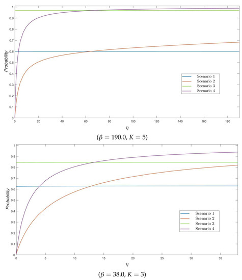
Figure 1. The probability $P({\eta }_{(i,z,a),K}<{\overline{\eta }}_{(i,z,a),0})$ as a function of $\eta$, for $N=50$.

In Figure 2, we plot the mean number of upcrossings to level $l\left(K\right)$, for $K=3$, as a function of $\eta$. We note that we always obtain, regardless of the parameters varied here, a relatively small mean number of upcrossings (e.g., less than $1.5$ in all scenarios). We point out that a mean number of upcrossings significantly below 1 means that the threshold number $K=3$ of varicella infective residents is not actually reached in most of the stochastic realizations of process $\mathcal{Y}$. This happens, for example, when a zoster infective resident starts the outbreak and there are control measures in place, so that the transmissibility of herpes zoster is low (i.e., relatively small values of $\eta$ in Figure 2). For large enough values of $\eta$, or for those scenarios in which a varicella infective resident starts the outbreak, a mean number of upcrossings relatively close to 1 illustrates how level $l\left(K\right)$ with $K=3$ is in fact reached during the early stages of the outbreak (i.e., while the number of infective residents is increasing over early times, moving towards its peak beyond $K=3$). Values of $E\left[{\mu }_{(i,z,a),K}\right]$ slightly above 1 illustrate the stochasticity of the epidemic process under analysis and might be explained by stochastic contributions from some particular realizations of the process (for example, if process $\mathcal{Y}$ reaches $K=3$ varicella infective residents, and one of these residents recovers before another infection immediately occurs, moving the process to level $l\left(2\right)$ before visiting level $l\left(3\right)$ again, and causing then two upcrossings).

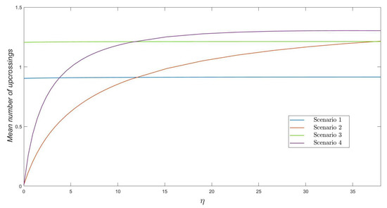
Figure 2. The mean number $E\left[{\mu }_{(i,z,a),K}\right]$ of upcrossings as a function of $\eta$, for $\beta =38.0$, $K=3$ and $N=50$.

In Figure 3, we plot the proportion of expected time $E\left[{\gamma }_{(i,z,a),K}\right]/E\left[{\overline{\eta }}_{(i,z,a),0}\right]$ that the process $\mathcal{Y}$ stays at or above level $l\left(K\right)$. This might be of interest since, for example, if K varicella infective residents represent an alert or warning level from which the nursing home needs to incur in some particular costs per unit time (e.g., particular enhanced control measures), the quantity $E\left[{\gamma }_{(i,z,a),K}\right]/E\left[{\overline{\eta }}_{(i,z,a),0}\right]$ would become an implicit quantification of this cost. We plot $E\left[{\gamma }_{(i,z,a),K}\right]/E\left[{\overline{\eta }}_{(i,z,a),0}\right]$ for a nursing home with some control strategies initially in place (so $\beta =38.0$), and for $K=3$ for illustrative purposes. The proportion of expected time spent above level $l\left(K\right)$ directly depends on who starts the outbreak (from either a varicella infective resident or a zoster infective resident) in the first place, the number of susceptible residents in the nursing home ($q=0.9$ versus $q=0.8$) and the zoster infectivity rate $\eta$. Proportions near to zero for Scenarios 2 and 4 and small values of $\eta$ are explained by the fact that level $l\left(3\right)$ is likely not reached in these situations. On the other hand, for increasing values of the infectivity rate $\eta$, the proportion of expected time spent above level $l\left(3\right)$ directly depends on how many susceptible residents stay in the nursing home (which allows for larger epidemic peaks beyond $K=3$ to be reached, likely leading to larger intervals of time until the epidemic curve decreases—by recoveries of infective residents—and goes again below level $l\left(3\right)$). Similar comments explain the behavior of Scenarios 1 and 3, but, in these, the impact of parameter $\eta$ is negligible since a varicella infective resident starts the outbreak.

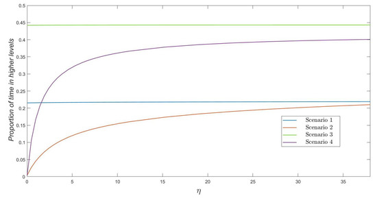
Figure 3. The proportion of expected time $E\left[{\gamma }_{(i,z,a),K}\right]/E\left[{\overline{\eta }}_{(i,z,a),0}\right]$ that process $\mathcal{X}$ spends at states in ${\cup }_{i=K}^{N}l\left(i\right)$ during an outbreak as a function of $\eta$, for $\beta =38.0$, $K=3$ and $N=50$.

In Figure 4, the interest is in the ratio $E\left[{\alpha }_{(i,z,a),0}\right]/(N·E\left[{\overline{\eta }}_{(i,z,a),0}\right])$, which represents the area under the curve of varicella infectious residents normalized by the total amount of time units that N residents stay at the nursing home during the varicella outbreak. We note here that this descriptor can be seen as a measure of cost, if, for example, the nursing home incurs in some costs per infective resident and per unit of time they remain infected. The behavior of this descriptor is similar to that observed in previous plots, whence we do not repeat preceding observations. However, we should emphasize here that the normalized area under the number of infectives is always less than the $7\%$ of the total cost during the outbreak –measured in terms of $N·E\left[{\overline{\eta }}_{(i,z,a),0}\right]$–, in such a way that the smallest and the highest values of the ratio $E\left[{\alpha }_{(i,z,a),0}\right]/(N·E\left[{\overline{\eta }}_{(i,z,a),0}\right])$ correspond to Scenarios 2 and 3, respectively, in our numerical experiments.

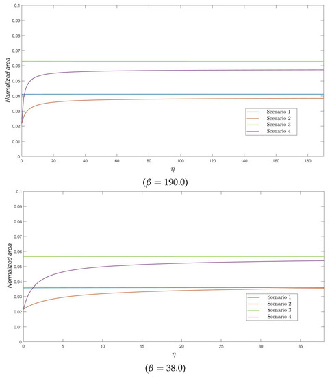
Figure 4. The ratio $E\left[{\alpha }_{(i,z,a),0}\right]/(N·E\left[{\overline{\eta }}_{(i,z,a),0}\right])$ as a function of $\eta$, for $N=50$.

6. Conclusions

In this paper, we extended the theory of finite QBD processes, given by Gaver et al. [1] by studying a number of random descriptors of interest which are defined inspired in their application to epidemic models, namely first-passage times and hitting probabilities to higher levels, number of upcrossings, and sojourn times, as well as the area under the level trajectory. We noted that these descriptors can have specific meanings when focusing on epidemic models: first-passage times and hitting probabilities can, for example, relate to the duration of an outbreak and the size of the epidemic, respectively; the number of upcrossings to a particular high level can represent the number of instances a particular threshold number of infectives is reached (which might lead to the introduction of particular control measures), while the area under the level trajectory can be translated into the area under the curve of infectives, a descriptor that has been analyzed before in the theory of mathematical epidemiology due to its potential interpretation in terms of the cost of a given outbreak. Although our results have been derived under the assumption that the finite QBD process is irreducible, they also hold under the less restrictive condition that $l\left(0\right)$ is accessible from the class ${\cup }_{i=1}^{N}l\left(i\right)$ of communicating states.

In order to analyze these stochastic descriptors or summary statistics, we considered auxiliary bi-dimensional absorbing processes in which infinitesimal generators are described in terms of levels and phases, and we presented a block-structured form of these generators. We were able to exploit this structure to determine recursive relations involving sub-matrices of these infinitesimal generators, in order to compute the quantities of interest in an iterative and efficient way. Our algorithmic solution involves recursive procedures and block-Gaussian elimination, whence the computational complexity of Algorithms A1–A6 (Appendix A, Appendix B, Appendix C and Appendix D) can be written in a similar manner to the computational complexity of the linear level reduction algorithm of Gaver et al. [1], and Algorithms 1.A–3.A of Gómez-Corral and López-García [29]. This makes the memory requirements of Algorithms A1–A6, especially for storing auxiliary matrices in Algorithm A1, very demanding even for moderate values of N depending of the number of phases per level.

To illustrate the applicability of both our analytical and computational results, we have presented a numerical study of an epidemic model for the transmission of varicella-zoster virus within a nursing home. There is clearly future work to be done on the joint distribution of the random vector $(I_{max},{\tau }_{max})$, where $I_{max}$ is the maximum number of residents who are simultaneously varicella infectious (i.e., the maximum of the level variable) and ${\tau }_{max}$ is the time taken to reach this maximum number during an outbreak, and on how to relate herd immunity to the phase variable in the study of vaccination strategies in the context of varicella-zoster virus infections. Among other interesting problems to be addressed in epidemic models are also the extension to a population with variable size or the assumption of non-exponential events. These would lead to QBD processes with infinitely many possible values of the level variable and/or the phase variable, and piecewise-deterministic Markov processes, respectively. In these frameworks, the study of the stochastic descriptors analyzed in Section 2, Section 3 and Section 4 should require an analytical treatment and related numerical procedures that will be substantially different from those used in this paper; in particular, the analysis of first-passage times and sojourn times could benefit from the approach described by Dolgopyat and Goldsheid [45], who obtain necessary and sufficient conditions for the existence of the density of the invariant measure for random walks when the environment is ergodic in both the transient and recurrent regimes. Another aspect that deserves further exploration is how the finite-dimensional linear algebra ideas in Section 2 and Section 3 could be replaced by some suitable extension to the QBD case of the Karlin-McGregor orthogonal polynomial/spectral representation by translating the arguments in Reference [46,47,48] for discrete time processes to continuous time.

References

- Gaver, D.P.; Jacobs, P.A.; Latouche, G. Finite birth-and-death models in randomly changing environments. Adv. Appl. Probab. 1984, 16, 715–731. [Google Scholar] [CrossRef]
- Baumann, H.; Sandmann, W. Steady state analysis of level dependent quasi-birth-and-death processes with catastrophes. Comput. Oper. Res. 2012, 39, 413–423. [Google Scholar] [CrossRef]
- Gun, L.; Makowski, A.M. Matrix-geometric solution for finite capacity queues with phase-type distributions. In Proceedings of the Performance 87, Brussels, Belgium, 7–9 December 1987; pp. 269–282. [Google Scholar]
- Perel, E.; Yechiali, U. Finite two layered queueing systems. Probab. Eng. Inform. Sci. 2016, 30, 492–513. [Google Scholar] [CrossRef]
- Ye, J.; Li, S.Q. Folding algorithm: A computational method for finite QBD processes with level-dependent transitions. IEEE Trans. Commun. 1994, 42, 625–639. [Google Scholar]
- Artalejo, J.R.; Gómez-Corral, A. Modelling communication systems with phase type service and retrial times. IEEE Commun. Lett. 2007, 11, 955–957. [Google Scholar] [CrossRef]
- Artalejo, J.R.; Lopez-Herrero, M.J. Cellular mobile networks with repeated calls operating in random environment. Comput. Oper. Res. 2010, 37, 1158–1166. [Google Scholar] [CrossRef]
- Chakravarthy, S.R.; Gómez-Corral, A. The influence of delivery times on repairable k-out-of-N systems with spares. Appl. Math. Model. 2009, 33, 2368–2387. [Google Scholar] [CrossRef]
- Moghaddass, R.; Zuo, M.J.; Wang, W. Availability of a general k-out-of-n:G system with non-identical components considering shut-off rules using quasi-birth–death process. Reliab. Eng. Syst. Safe 2011, 96, 489–496. [Google Scholar] [CrossRef]
- Amador, J.; Gómez-Corral, A. A stochastic epidemic model with two quarantine states and a limited carrying capacity for quarantine. Phys. A Stat. Mech. Appl. 2020, 544, 121899. [Google Scholar] [CrossRef]
- Artalejo, J.R.; Economou, A.; Lopez-Herrero, M.J. The stochastic SEIR model before extinction: Computational approaches. Appl. Math. Comput. 2015, 265, 1026–1043. [Google Scholar] [CrossRef]
- Economou, A.; Gómez-Corral, A.; López-García, M. A stochastic SIS epidemic model with heterogeneous contacts. Phys. A Stat. Mech. Appl. 2015, 421, 78–97. [Google Scholar] [CrossRef]
- Gamboa, M.; Lopez-Herrero, M.J. Measuring infection transmission in a stochastic SIV model with infection reintroduction and imperfect vaccine. Acta Biotheor. 2020, in press. [Google Scholar] [CrossRef] [PubMed]
- Latouche, G.; Ramaswami, V. Introduction to Matrix Analytic Methods in Stochastic Modeling; ASA-SIAM: Philadelphia, PA, USA, 1999. [Google Scholar]
- Hajek, B. Birth-and-death processes on the integers with phases and general boundaries. J. Appl. Probab. 1982, 19, 488–499. [Google Scholar] [CrossRef]
- Akar, N.; Oğuz, N.C.; Sohraby, K. A novel computational method for solving finite QBD processes. Stoch. Models 2000, 16, 273–311. [Google Scholar] [CrossRef]
- Stewart, W.J. Introduction to the Numerical Solutions of Markov Chains; Princeton University Press: Princeton, NJ, USA, 1994. [Google Scholar]
- Naoumov, V. Modified matrix-geometric solution for finite QBD processes. In Advances in Algorithmic Methods for Stochastic Models; Latouche, G., Taylor, P.G., Eds.; Notable Publications, Inc.: Upper Saddle River, NJ, USA, 2000; pp. 257–263. [Google Scholar]
- Li, Q.L.; Cao, J. Two types of RG-factorizations of quasi-birth-and-death processes and their applications to stochastic integral functionals. Stoch. Models 2004, 20, 299–340. [Google Scholar] [CrossRef]
- Elhafsi, E.H.; Molle, M. On the solution to QBD processes with finite state space. Stoch. Anal. Appl. 2007, 25, 763–779. [Google Scholar] [CrossRef]
- De Nitto Personè, V.; Grassi, V. Solution of finite QBD processes. J. Appl. Probab. 1996, 33, 1003–1010. [Google Scholar] [CrossRef]
- Le Boudec, J.Y. An efficient solution method for Markov models of ATM links with loss priorities. IEEE J. Sel. Areas Comm. 1991, 9, 408–417. [Google Scholar] [CrossRef]
- Da Silva Soares, A.; Latouche, G. The group inverse of finite homogeneous QBD processes. Stoch. Models 2002, 18, 159–171. [Google Scholar] [CrossRef]
- Baumann, H.; Sandmann, W. Numerical solution of level dependent quasi-birth-and-death processes. Procedia Comput. Sci. 2012, 2012 1, 1561–1569. [Google Scholar] [CrossRef]
- Li, S.Q.; Sheng, H.D. Generalized folding-algorithm for sojourn time analysis of finite QBD processes and its queueing applications. Stoch. Models 1996, 12, 507–522. [Google Scholar]
- Shin, Y.W. Fundamental matrix of transient QBD generator with finite states and level dependent transitions. Asia Pac. J. Oper. Res. 2009, 26, 697–714. [Google Scholar] [CrossRef]
- Neuts, M.F. Matrix-Geometric Solutions in Stochastic Models: An Algorithmic Approach; The Johns Hopkins University Press: Baltimore, MD, USA, 1981. [Google Scholar]
- Artalejo, J.R.; Gómez-Corral, A. Retrial Queueing Systems: A Computational Approach; Springer: Berlin, Germany, 2008. [Google Scholar]
- Gómez-Corral, A.; López-García, M. Perturbation analysis in finite LD-QBD processes and applications to epidemic models. Numer. Linear Algebr. Appl. 2018, 2018, e2160. [Google Scholar] [CrossRef] [PubMed]
- Amador, J.; Armesto, D.; Gómez-Corral, A. Extreme values in SIR epidemic models with two strains and cross-immunity. Math. Biosci. Eng. 2019, 16, 1992–2022. [Google Scholar] [CrossRef] [PubMed]
- Baumann, H.; Sandmann, W. Structured modeling and analysis of stochastic epidemics with immigration and demographic effects. PLoS ONE 2016, 11, e0152144. [Google Scholar] [CrossRef] [PubMed]
- Lefèvre, C.; Simon, M. SIR-type epidemic models as block-structured Markov processes. Methodol. Comput. Appl. Probab. 2020, 22, 433–453. [Google Scholar] [CrossRef]
- Neuts, M.F.; Li, J.M. An algorithmic study of S-I-R stochastic epidemic models. In Athens Conference on Applied Probability and Time Series Analysis. Volume I: Applied Probability In Honor of J.M. Gani. Lecture Notes in Statistics, Volume 114; Heyde, C.C., Prohorov, Y.V., Pyke, R., Rachev, S.T., Eds.; Springer: New York, NY, USA, 1996; pp. 295–306. [Google Scholar]
- Hunter, J.J. Mathematical Techniques of Applied Probability. Volume 1, Discrete Time Models: Basic Theory; Academic Press: New York, NY, USA, 1983. [Google Scholar]
- Downton, F. The area under the infectives trajectory of the general stochastic epidemic. J. Appl. Probab. 1972, 9, 414–417. [Google Scholar] [CrossRef]
- Gani, J.; Jerwood, D. The cost of a general stochastic epidemic. J. Appl. Probab. 1972, 9, 257–269. [Google Scholar] [CrossRef]
- Ball, F. A unified approach to the distribution of total size and total area under the trajectory of infectives in epidemic models. Adv. Appl. Probab. 1986, 18, 289–310. [Google Scholar] [CrossRef]
- Comba, M.; Martorano-Raimundo, S.; Venturino, E. A cost-effectiveness-assessing model of vaccination for varicella and zoster. Math. Model. Nat. Phenom. 2012, 7, 62–77. [Google Scholar] [CrossRef]
- Forder, J.; Fernandez, J.-L. Length of Stay in Care Homes; Report Commissioned by Bupa Care Services; PSSRU Discussion Paper 2769; PSSRU: Canterbury, UK, 2011; Volume 2769. [Google Scholar]
- Froggatt, K.; Edwards, M.; Morbey, H.; Payne, S. Mapping Palliative Care Systems in Long Term Care Facilities in Europe; PACE Work Package 1 and EAPC Taskforce Report; Palliative Care Older People, Lancaster University: Lancaster, UK, 2016. [Google Scholar]
- Cohen, K.R.; Salbu, R.L.; Frank, J.; Israel, I. Presentation and management of herpes zoster (shingles) in the geriatric population. Pharm. Therap. 2013, 38, 217–227. [Google Scholar]
- Zussman, J.; Young, L. Zoster vaccine live for the prevention of shingles in the elderly patient. Clin. Interv. Aging 2008, 3, 241–250. [Google Scholar] [PubMed]
- Mueller, N.H.; Gilden, D.H.; Cohrs, R.J.; Mahalingam, R.; Nagel, M.A. Varicella zoster virus infection: Clinical features, molecular pathogenesis of disease, and latency. Neurol. Clin. 2008, 26, 675–697. [Google Scholar] [CrossRef] [PubMed]
- Nardone, A.; de Ory, F.; Carton, M.; Cohen, D.; van Damme, P.; Davidkin, I.; Rota, M.C.; de Melker, H.; Mossong, J.; Slacikova, H.; et al. The comparative sero-epidemiology of varicella zoster virus in 11 countries in the European region. Vaccine 2007, 25, 7866–7872. [Google Scholar] [CrossRef]
- Dolgopyat, D.; Goldsheid, I. Invariant measure for random walks on ergodic environments on a strip. Ann. Probab. 2019, 47, 2494–2528. [Google Scholar] [CrossRef]
- Castro, M.M.; Grünbaum, F.A. On a seminal paper by Karlin and McGregor. SIGMA 2013, 9, 020. [Google Scholar] [CrossRef]
- Coolen-Schrijner, P.; van Doorn, E.A. Analysis of random walks using orthogonal polynomials. J. Comp. Appl. Math. 1998, 99, 387–399. [Google Scholar] [CrossRef]
- Kovchegov, Y. Orthogonality and probability: Beyond nearest neighbor transitions. Electron. Commun. Probab. 2009, 14, 90–103. [Google Scholar] [CrossRef]
© 2020 by the authors. Licensee MDPI, Basel, Switzerland. This article is an open access article distributed under the terms and conditions of the Creative Commons Attribution (CC BY) license (http://creativecommons.org/licenses/by/4.0/).