The Basic Algorithm for the Constrained Zero-One Quadratic Programming Problem with k-diagonal Matrix and Its Application in the Power System

Abstract

Zero-one quadratic programming is a classical combinatorial optimization problem that has many real-world applications. However, it is well known that zero-one quadratic programming is non-deterministic polynomial-hard (NP-hard) in general. On one hand, the exact solution algorithms that can guarantee the global optimum are very time consuming. And on the other hand, the heuristic algorithms that generate the solution quickly can only provide local optimum. Due to this reason, identifying polynomially solvable subclasses of zero-one quadratic programming problems and their corresponding algorithms is a promising way to not only compromise these two sides but also offer theoretical insight into the complicated nature of the problem. By combining the basic algorithm and dynamic programming method, we propose an effective algorithm in this paper to solve the general linearly constrained zero-one quadratic programming problem with a k-diagonal matrix. In our algorithm, the value of k is changeable that covers different subclasses of the problem. The theoretical analysis and experimental results reveal that our proposed algorithm is reasonably effective and efficient. In addition, the placement of the phasor measurement units problem in the power system is adopted as an example to illustrate the potential real-world applications of this algorithm.

1. Introduction

Optimization problems normally fall into two categories, one for continuous variables and the other for discrete variables. The latter one is called combinatorial optimization, which is an active field in applied mathematics [1]. Common problems are the maximum flow problem, traveling salesman problem, matching problem, knapsack problem, etc. Among those famous combinatorial optimizations, zero-one quadratic programming (01QP), whose variables can only be either 0 or 1 [2], is very important and attracts a lot of attention.

Zero-one quadratic programming, which can be divided into constrained (01CQP) and unconstrained (01UQP), is a combinatorial optimization and has practical significance. For example, it can be applied in circuit design [3], pattern recognition [4], capital budgeting [5], portfolio optimization [6], etc. Except for these well known applications, 01QP also has potential applications in the nonlinear control related fields [7,8,9,10,11]. Among these applications, the phasor measurement unit (PMU) placement has been widely studied. Phasor measurement units can be used in dynamic monitoring, system protection, and system analysis and prediction. Therefore, the placement of PMU has become an important issue. As the scale of the electric grid grows, the PMU placement problem becomes more difficult and must be addressed considering certain requirements. In [12], a modified bisecting search combined with simulated annealing method was proposed, and the latter randomly selected arrays were used to test the observability of the system. Considering the incomplete observability of the system, a calculation method based on graph theory was proposed in [13]. This method is time-consuming, and with the increase of dimensions, the calculation load is too heavy. An integer linear programming method [14] and an improved algorithm [15] were put forward, considering system redundancy, and full and incomplete observability. Researchers in [16] proposed a binary programming method considering the joint placement of the conventional measurement units and phasor measurement units.

Zero-one quadratic programming also has some theoretical significance. Many classical problems, such as the max-cut problem [17,18] and max-bisection problem [19] can be converted to zero-one quadratic programming. Therefore, designing the algorithm that can solve 01QP effectively and efficiently is very meaningful not only in practical fields but also in theoretical fields.

However, zero-one quadratic programming is a well known NP-hard problem in general. The common solutions are exact solution and heuristic algorithms. Exact solution algorithms can guarantee the global optimum. In [20], the branch-and-bound method was used to solve zero-one quadratic programming problems without constraints. In [21,22], some exact solutions were proposed by means of geometric properties. Penalty parameters were introduced to solve zero-one quadratic programming problems with constraints in [23]. But exact solution algorithm are very time consuming and suitable for small scale problems only. Oppositely, heuristic algorithms, such as simulated annealing [24], genetic algorithms [25], neural networks [26], and ant colony algorithms [27], can solve the medium and large scale problems quickly in general. But most of them can only find the local optimum.

Therefore, identifying polynomially solvable subclasses of zero-one quadratic programming problems and their corresponding algorithms is a promising way to not only compromise these two sides but also offer theoretical insight into the complicated nature of the problem. In our past studies [28,29], the problem of five-diagonal matrix quadratic programming with linear constraints has been solved effectively. In [30], an algorithm for solving 01QP with a seven-diagonal matrix Q was presented. However, for these algorithms, the applicable problem is very specific. This narrows their applications. Then, we proposed an algorithm for the unconstrained problems with a k-diagonal matrix in [31]. In this paper, based on our previous results, we further propose an algorithm for the general linearly constrained zero-one quadratic programming problem with a k-diagonal matrix by combining the basic algorithm and dynamic programming method. For the algorithm we proposed, the value of k is changeable. That means the algorithm can cover different subclasses of the problem. The theoretical analysis and experimental results reveal that our proposed algorithm is reasonably effective and efficient. We also apply the algorithm to real-world applications and then verify its feasibility.

The main contributions of this paper are reflected in the following aspects: (1) The previous algorithm targeted a fixed k value in Q matrix. While the algorithm in this paper targeted a general problem with changeable k values. (2) We analyze the time complexity and give the proof process of the rationality of the algorithm. (3) We apply the algorithm to the phasor measurement units placement in real-world application.

This paper is organized as follows: in Section 2, we review the algorithm of solving unconstrained zero-one k-diagonal matrix quadratic programming. In Section 3, a constrained zero-one k-diagonal matrix quadratic programming algorithm with the proof of the algorithm is proposed. Application of zero-one quadratic programming in the phasor measurement units placement is put forward in Section 4. Experimental results and discussion are given in Section 5. We draw our conclusions and put forward the prospects in Section 6.

2. Basic Algorithm to 01UQP

The following Equation (1) shows the form of the k-diagonal matrix zero-one quadratic programming problem. The special point is the form of the matrix Q called the k-diagonal matrix, where $k=2m+1$$(m=0,1,2,\dots ,n-1)$.

$$\begin{array}{cc}\hfill & \underset{x\in {\{0,1\}}^n}{min}f\left(x\right)=\frac{1}{2}{x}^{T}Qx+c^{T}x\hfill \end{array}$$

(1)

where $Q={\left(q_{ij}\right)}_{n\times n}$, $q_{ij}=q_{ji}(i,j=1,2,\dots ,n)$ indicates that it is a symmetric matrix. Note that all the numbers in this matrix are zero except $q_{ij}$ and $q_{ji}$$(i=1,2,\dots ,n-1,j=i+1,i+2,\dots ,i+m)$.

$$\left(\begin{array}{ccccccc}0& q_{1,2}& q_{1,3}& \cdots & 0& 0& 0\\ q_{2,1}& 0& q_{2,3}& \cdots & 0& 0& 0\\ q_{3,1}& q_{3,2}& 0& \cdots & 0& 0& 0\\ ⋮& ⋮& ⋮& \ddots & ⋮& ⋮& ⋮\\ 0& 0& 0& \cdots & 0& q_{n-2,n-1}& q_{n-2,n}\\ 0& 0& 0& \cdots & q_{n-1,n-2}& 0& q_{n-1,n}\\ 0& 0& 0& \cdots & q_{n,n-2}& q_{n,n-1}& 0\end{array}\right)$$

Based on past works [30,31], we can have the algorithm, as follows, to solve 01UQP. The feasibility and effect of the algorithm can be seen in [31]. Figure 1 shows the Algorithm 1 process intuitively.

Algorithm 1 Process of solving 01UQP

Step 1:  Assign $x_{n-m+1}$,…, $x_n$ to 0 or 1. (1) Adjacent terms are the combination of $x_{n-m+1}$,…, $x_n$, whose value is the same except for the value of $x_n$. (2) Get the corresponding $f\left(x\right)$. (3) Label these states $state0,state1,\dots ,state(2^m-1)$. (4) Compare $f\left(x\right)$ in the two adjacent terms. (only the coefficient of $x_{n-m}$ and the constant term are different.) Step 2:  Change the value of $x_{n-m-i}$ to 0 and 1($i=0,1,\dots ,n-m-1$). (1) Compare every two adjacent states and take the result with the smaller constant term as the new state. (2) Update all the $2^m$ states. Step 3:  Get the optimal solution x. (1) Update the states based on Step 2 until only the constant term is in $f\left(x\right)$. (2) The optimal value is the minimal one. (3) Trace back and get the optimal solution x.

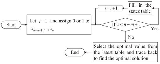
Figure 1. Flow chart of the zero-one unconstrained quadratic programming (01UQP) algorithm.

3. Basic Algorithm to 01CQP

3.1. 01CQP Algorithm Description

Consider the constrained k-diagonal matrix zero-one quadratic programming problem:

$$\begin{array}{cc}\underset{x\in {\{0,1\}}^n}{\min }\hfill & \frac{1}{2}{x}^{T}Qx+c^{T}x\hfill \\ \mathrm{s}.\mathrm{t}.\hfill & a^{T}x\le b\hfill \end{array}$$

(2)

where Q has the same meaning as that of the 01UQP formula in Section 2, $a\in {\mathbb{Z}}_{+}^n$, $b\in {\mathbb{Z}}_{+}$.

In this section, we utilize the dynamic programming method to solve the 01CQP problem. To apply the dynamic programming method, we introduce a state variable $s_k(s_k\in \mathbb{Z})$ and a stage variable $k(0<k\le n)$, which should satisfy the following iteration. $s_{k+1}$ can be expressed as:

$$\begin{array}{c}\hfill s_{k+1}=s_k+a_{k+1}{x}_{k+1}(k=1,\dots ,n-1)\end{array}.$$

We only need to consider the integer point of the state space since $a\in {\mathbb{Z}}_{+}^n$ and $b\in {\mathbb{Z}}_{+}$. Since $s_k$ satisfies $0\le s_k\le b$, we define a set $s_k=\left\{s_k\right|0\le s_k\le b,s_k\in \mathbb{Z}\}$.

Algorithms 2 and 3 show the detailed calculation process.

Algorithm 2 Calculation Method of $f\left(s_k\right)$

Case 1:  When $k=1$, there are two cases. (1a)$s_1<a_1$ $x_1=0$, $x_1^{*}=0$, $f\left(s_1\right)=f(0,\dots ,x_n)$ (1b)$s_1\ge a_1$ $x_1=1$, $x_1^{*}=1$, $f\left(s_1\right)=f(1,\dots ,x_n)$ We will get a series of functions $f\left(x\right)$ after executing Case 1. Case 2:  When $k\ge 2$, there are also two cases. (2a)$s_k<a_k$ $x_k$ must be 0 to satisfy $s_{k-1}=s_k-a_k{x}_k$. At this time, $s_k=s_{k-1}$, by which we can obtain the function $f\left(s_k\right)=f\left(s_{k-1}\right){|}_{x_k=0}$. (2b)$s_k\ge a_k$ In this case, $x_k$ can be both 0 or 1, which generates two more situations: 1) If ${x_k}^{*}=0$ and $s_k=s_{k-1}$, we can get $f\left(s_k\right)=f\left(s_{k-1}\right){|}_{x_k=0}$. 2) If ${x_k}^{*}=1$ and $s_{k-1}=s_k-a_k{x}_k$, we can get $f\left(s_k\right)=f\left(s_{k-1}\right){|}_{x_k=1}$. We can see that there is only one function $f\left(s_k\right)$ corresponding to each state $s_k$ when $k=1$, and there are several $f\left(s_k\right)$ to each state $s_k$ when $k>1$. To save storage and computational time, $f\left(s_k\right)$ should be selected satisfactorily in the next step. We need to find the optimal $f\left(s_k\right)=f\left(s_{k-1}\right){|}_{x_k=0}$ and $f\left(s_k\right)=f\left(s_{k-1}\right){|}_{x_k=1}$, that the optimizing process refers to for Algorithm 3.

Algorithm 3$stat{e}_0$ and $stat{e}_1$

$stat{e}_0(x_k=0)$             Case 1: There is only one $f\left(s_k\right)=f\left(s_{k-1}\right){|}_{x_k=0}$:             Set ${x_k}^{*}=0$, $f\left(s_k\right)=f\left(s_{k-1}\right){|}_{x_k=0}$             Case 2: There are more than one $f\left(s_k\right)=f\left(s_{k-1}\right){|}_{x_k=0}$:             1) Compare $f\left(s_{k-1}\right){|}_{x_k=0}$, which are almost the same except for the constant term and pick up the smallest one.             2) Set ${x_k}^{*}=0$ and $f\left(s_k\right)=f\left(s_{k-1}\right){|}_{x_k=0}$. $stat{e}_1(x_k=1)$             Case 1: There is only one $f\left(s_k\right)=f\left(s_{k-1}\right){|}_{x_k=1}$:             Set ${x_k}^{*}=1$, $f\left(s_k\right)=f\left(s_{k-1}\right){|}_{x_k=1}$             Case 2: There are more than one $f\left(s_k\right)=f\left(s_{k-1}\right){|}_{x_k=1}$:             1) Find the $f\left(x\right)$ using a similar approach to that in $stat{e}_0$ Case 2.             2) Set ${x_k}^{*}=1$ and $f\left(s_k\right)=f\left(s_{k-1}\right){|}_{x_k=1}$.

According to the above algorithm, the maximum number of functions per $State$ is shown in Table 1. The primary time is spent generating the state table. The number of times that the core steps calculated is focused on the state number in Table 1. In total, we need to update the state table n times and the number of state is b, so the time complexity is $O(2^{m-1}\times n\times b)$.

Table 1. Maximum number of functions per $State$.

Situation	The Maximum Number of Functions
Algorithm 2 Case 1	1
Algorithm 3 Case 1	$2^{m-1}$
Algorithm 3 Case 2	$2^{m-1}$

3.2. Analysis on the Effectiveness and Rationality of 01CQP Algorithm

In this section, we analyze the properties of the polynomial time algorithm for 01CQP. To analyze the algorithm, we need to demonstrate the rationality of Algorithms 2 and 3. Suppose $f\left(x\right)$ has the form:

$$\begin{array}{c}\hfill \begin{array}{c}f\left(x\right)=q_{12}{x}_1{x}_2+q_{13}{x}_1{x}_3+\cdots +q_{1,1+m}{x}_1{x}_{1+m}+\cdots +q_{n-m,n-m+1}{x}_{n-m}\hfill \\ x_{n-m+1}+\cdots +q_{n-m,n}{x}_{n-m}{x}_n+\cdots +q_{n-1,n}{x}_{n-1}{x}_n+c_1{x}_1+\cdots +c_n{x}_n.\hfill \end{array}\end{array}$$

Step 1: Set $k=1$

(1) $s_1<a_1,x_1=0$

$$\begin{array}{c}\hfill \begin{array}{c}{f}_1\left(s_1\right)=f\left(x\right){|}_{x_1=0}=q_{i,i+1}{x}_i{x}_{i+1}+q_{i,i+2}{x}_i{x}_{i+2}+\cdots +q_{i,i+m}{x}_i{x}_{i+m}\hfill \\ +\cdots +q_{n-m,n-m+1}{x}_{n-m}{x}_{n-m+1}+\cdots +q_{n-m,n}{x}_{n-m}{x}_n\hfill \\ +\cdots +q_{n-1,n}{x}_{n-1}{x}_n+c_2{x}_2+\cdots +c_n{x}_n(i=2,\dots ,n-m-1).\hfill \end{array}\end{array}$$

(3)

(2) $s_1\ge a_1,x_1=1$

$$\begin{array}{c}{f}_1\left(s_1\right)=f\left(x\right){|}_{x_1=1}=q_{i,i+1}{x}_i{x}_{i+1}+q_{i,i+2}{x}_i{x}_{i+2}+\cdots +q_{i,i+m}{x}_i{x}_{i+m}\hfill \\ +\cdots +q_{n-m,n-m+1}{x}_{n-m}{x}_{n-m+1}+\cdots +q_{n-m,n}{x}_{n-m}{x}_n\hfill \\ +\cdots +q_{n-1,n}{x}_{n-1}{x}_n+\widehat{c_2}{x}_2+\cdots +\widehat{c_{1+m}}{x}_{1+m}+c_{m+2}{x}_{m+2}\hfill \\ +\cdots +c_n{x}_n+c_1.\hfill \end{array}$$

(4)

Clearly, when $k=1$, each state $s_1$ has only one function $f_1\left(s_1\right)$. The coefficient of $x_2,\dots ,x_{m+1}$ and the constants are the only different terms in the function.

Step 2: Set $k=2,3,\dots m$

(1) If $s_k<a_k$, execute $stat{e}_0$.

If $s_{k-1}<a_{k-1}$, $f_k\left(s_k\right)$ has the same form as function (3):

$$\begin{array}{c}f\left(s_k\right)=q_{k,k+1}{x}_k{x}_{k+1}+q_{k,k+2}{x}_k{x}_{k+2}+\cdots +q_{k,k+m}{x}_k{x}_{k+m}\hfill \\ +\cdots +q_{i,i+1}{x}_i{x}_{i+1}+q_{i,i+2}{x}_i{x}_{i+2}+\cdots +q_{i,i+m}{x}_i{x}_{i+m}+\cdots +\hfill \\ q_{n-m,n-m+1}{x}_{n-m}{x}_{n-m+1}+\cdots +q_{n-m,n}{x}_{n-m}{x}_n+\cdots +\hfill \\ q_{n-1,n}{x}_{n-1}{x}_n+c_{k+1}{x}_{k+1}+\cdots +c_n{x}_n+const.\hfill \end{array}$$

(5)

($const$ represents the constant term of the $f\left(s_{k-1}\right)$.)

If $s_k\ge a_{k-1}$, $f_k\left(s_k\right)$ has the same form as function (4):

$$\begin{array}{c}f\left(s_{k-1}\right)=q_{k,k+1}{x}_k{x}_{k+1}+q_{k,k+2}{x}_k{x}_{k+2}+\cdots +q_{k,k+m}{x}_k{x}_{k+m}\hfill \\ +\cdots +q_{i,i+1}{x}_i{x}_{i+1}+q_{i,i+2}{x}_i{x}_{i+2}+\cdots +q_{i,i+m}{x}_i{x}_{i+m}+\cdots +\hfill \\ q_{n-m,n-m+1}{x}_{n-m}{x}_{n-m+1}+\cdots +q_{n-m,n}{x}_{n-m}{x}_n+\cdots +\hfill \\ q_{n-1,n}{x}_{n-1}{x}_n+\widehat{c_{k+1}}{x}_{k+1}+\cdots +\widehat{c_{k+m}}{x}_{k+m}+c_{k+m}{x}_{k+m}\hfill \\ +\dots +c_n{x}_n+const+c_k.\hfill \end{array}$$

(6)

Then, $f_k\left(s_k\right)$ can be shown as:

$$\begin{array}{c}{f}_k\left(s_k\right)=f_{k-1}\left(s_{k-1}\right){|}_{x_k=0}=q_{k+1,k+2}{x}_{k+1}{x}_{k+2}+q_{k+1,k+3}{x}_{k+1}{x}_{k+3}+\cdots \hfill \\ +q_{k+1,k+m+1}{x}_{k+1}{x}_{k+m+1}+\cdots +q_{i,i+1}{x}_i{x}_{i+1}+q_{i,i+2}{x}_i{x}_{i+2}+\cdots +\hfill \\ q_{i,i+m}{x}_i{x}_{i+m}+\cdots +q_{n-m,n-m+1}{x}_{n-m}{x}_{n-m+1}+\cdots +q_{n-m,n}{x}_{n-m}{x}_n\hfill \\ +\cdots +q_{n-1,n}{x}_{n-1}{x}_n+\widehat{c_{k+1}}{x}_{k+1}+\cdots +\widehat{c_{k+m}}{x}_{k+m}+c_{k+m+1}{x}_{k+m+1}\hfill \\ +\dots +c_n{x}_n+\widehat{const}.\hfill \end{array}$$

(7)

At this point, the maximum number of $f_k\left(s_k\right)$ corresponding to each $s_k$ is $2^{k-2}$.

(2) If $s_k\ge a_k$, execute $stat{e}_0$ and $stat{e}_1$.

Here, the $stat{e}_0$ is the same as the one in Case 1, so we do not need to repeat it.

Consider $stat{e}_1,x_k=1$, $f_k\left(s_k\right)=f_{k-1}(s_k-a_k{x}_k)$, $s_{k-1}=s_k-a_k{x}_k=s_k-a_k$.

If $s_{k-1}<a_{k-1}$, $f\left(s_{k-1}\right)$ has the form of function (5). If $s_{k-1}\ge a_{k-1}$, $f\left(s_{k-1}\right)$ has the form of function (6), then, $f_k\left(s_k\right)$ can be expressed as:

$$\begin{array}{c}{f}_k\left(s_k\right)=f_{k-1}\left(s_{k-1}\right){|}_{x_k=1}=q_{k+1,k+2}{x}_{k+1}{x}_{k+2}+q_{k+1,k+3}{x}_{k+1}{x}_{k+3}+\cdots \hfill \\ +q_{k+1,k+m+1}{x}_{k+1}{x}_{k+m+1}+\cdots +q_{i,i+1}{x}_i{x}_{i+1}+q_{i,i+2}{x}_i{x}_{i+2}+\cdots +\hfill \\ q_{i,i+m}{x}_i{x}_{i+m}+\cdots +q_{n-m,n-m+1}{x}_{n-m}{x}_{n-m+1}+\cdots +q_{n-m,n}{x}_{n-m}{x}_n\hfill \\ +\cdots +q_{n-1,n}{x}_{n-1}{x}_n+{\widehat{c_{k+1}}}^{{}^{\prime }}{x}_{k+1}+\cdots +{\widehat{c_{k+m}}}^{{}^{\prime }}{x}_{k+m}+c_{k+m+1}{x}_{k+m+1}\hfill \\ +\dots +c_n{x}_n+{\widehat{const}}^{{}^{\prime }}.\hfill \end{array}$$

(8)

All $f_k\left(s_k\right)$ are only different in the constant terms and the coefficient of $x_{k+1},\dots ,x_{m+2}$.

Step 3:$k=n-m-1$

Consider the most complex case, $s_k\ge a_k$ and the state variable $s_k$ corresponds to $2^{m-1}$$f_k\left(s_k\right)$ and $2^{m-1}$$f_k\left(s_k\right)=f_{k-1}(s_k-a_k)$ respectively ($2^{m-1}$ is the number of both). Therefore, we need to execute $stat{e}_0$ first, and then execute $stat{e}_1$.

(1) $stat{e}_0$:

Since $f_k\left(s_k\right)$ has the form as function (8), the $stat{e}_0$ is executed for the $f_k\left(s_k\right)$ respectively, and the following expression is obtained:

$$\begin{array}{c}{f}_k\left(s_k\right)=f_{k-1}\left(s_k\right){|}_{x_k=0}=q_{n-m,n-m+1}{x}_{n-m}{x}_{n-m+1}+\cdots +\hfill \\ q_{n-m,n}{x}_{n-m}{x}_n+\cdots +q_{n-1,n}{x}_{n-1}{x}_n+{\widehat{c_{n-m}}}^{{}^{\prime }}{x}_{n-m}+c_{n-m+1}{x}_{n-m+1}\hfill \\ +\dots +c_n{x}_n+{\widehat{const}}^{{}^{\prime }}.\hfill \end{array}$$

(9)

Clearly, these $f_k\left(s_k\right)$ are only different in the constants and the coefficients of $x_{n-m}$.

(2) $stat{e}_1$:

It is possible to obtain $f_k\left(s_k\right)$, which has the following form:

$$\begin{array}{c}{f}_k\left(s_k\right)=f_{k-1}\left(s_{k-1}\right){|}_{x_k=1}=q_{n-m,n-m+1}{x}_{n-m}{x}_{n-m+1}+\cdots +\hfill \\ q_{n-m,n}{x}_{n-m}{x}_n+\cdots +q_{n-1,n}{x}_{n-1}{x}_n+{\widehat{c_{n-m}}}^{{}^{″}}{x}_{n-m}+c_{n-m+1}{x}_{n-m+1}\hfill \\ +\dots +c_n{x}_n+{\widehat{const}}^{{}^{\prime }}+\widehat{c_{n-m-1}}.\hfill \end{array}$$

(10)

For both case (1) and (2), they are only different in the constants and the coefficients of $x_{k+1}$.

Step 4:$k=m+2,\dots ,n$

Based on Algorithm 2 Case 2, we calculate the function $f_k\left(s_k\right)$, and the core is the implementation of $stat{e}_0$ and $stat{e}_1$. When executing $stat{e}_0$ and $stat{e}_1$, the difference between the two $f_k\left(s_k\right)$ is the constant and the coefficients of $x_k$. Therefore, when executing $stat{e}_0$, we only need to compare the constant terms. When executing $stat{e}_1$, we only need to compare the sum of the constants and the coefficients of $x_k$. In this way, we can avoid solving the excess $f_k\left(s_k\right)$.

The form of the function $f_k\left(s_k\right)$ and the maximum number of $f_k\left(s_k\right)$ in each stage k are similar to the one in stage $k=n-m$, which also ensures the repeatability of the algorithm. The algorithm is supplemented by concrete examples and numerical simulations.

3.3. Calculation Example of 01CQP

For example, the parameters Q, c, a, and b are:

$$\begin{array}{cc}\hfill Q& =\left(\begin{array}{cccccccc}0& 23& -37& -56& 0& 0& 0& 0\\ 23& 0& 41& 16& -34& 0& 0& 0\\ -37& 41& 0& -62& -27& 76& 0& 0\\ -56& 16& -62& 0& -81& 14& -58& 0\\ 0& -34& -27& 81& 0& 90& 25& -42\\ 0& 0& 76& 14& 90& 0& -12& 31\\ 0& 0& 0& -58& 25& -12& 0& -94\\ 0& 0& 0& 0& -42& 31& -94& 0\end{array}\right)\hfill \\ \hfill c& ={\left(\begin{array}{cccccccc}24,& -54,& -17,& 36,& -72,& 63,& 46,& -18\end{array}\right)}^T\hfill \\ \hfill a& ={\left(\begin{array}{cccccccc}1,& 2,& 3,& 2,& 4,& 2,& 3,& 2\end{array}\right)}^T\hfill \\ \hfill b& =6.\hfill \end{array}$$

In this example, we will omit some of the states.

(1) Set $k=1$, $s_1=a_1{x}_1$,$a_1=1$

We can set $s_1=0,1,\dots ,6$. According to Algorithm 2 Case 1, we can obtain Table 2.

Table 2. Functions $f_1\left(s_1\right)$.

${\mathit{s}}_1$	${\mathit{x}}_1$	${\mathit{f}}_1\left({\mathit{s}}_1\right)({\mathit{a}}_1=1)$
0	0	$\begin{array}{c}41x_2{x}_3+16x_2{x}_4-34x_2{x}_5-62x_3{x}_4-27x_3{x}_5+76x_3{x}_6-81x_4{x}_5\hfill \\ +14x_4{x}_6-58x_4{x}_7+90x_5{x}_6+25x_5{x}_7-42x_5{x}_8-12x_6{x}_7+31x_6{x}_8\hfill \\ -94x_7{x}_8-54x_2-17x_3+36x_4-72x_5+63x_6+46x_7-18x_8\hfill \end{array}$
1	1	$\begin{array}{c}41x_2{x}_3+16x_2{x}_4-34x_2{x}_5-62x_3{x}_4-27x_3{x}_5+76x_3{x}_6-81x_4{x}_5\hfill \\ +14x_4{x}_6-58x_4{x}_7+90x_5{x}_6+25x_5{x}_7-42x_5{x}_8-12x_6{x}_7+31x_6{x}_8\hfill \\ -94x_7{x}_8-31x_2-54x_3-20x_4-72x_5+63x_6+46x_7-18x_8+24\hfill \end{array}$
2	1	$\begin{array}{c}41x_2{x}_3+16x_2{x}_4-34x_2{x}_5-62x_3{x}_4-27x_3{x}_5+76x_3{x}_6-81x_4{x}_5\hfill \\ +14x_4{x}_6-58x_4{x}_7+90x_5{x}_6+25x_5{x}_7-42x_5{x}_8-12x_6{x}_7+31x_6{x}_8\hfill \\ -94x_7{x}_8-31x_2-54x_3-20x_4-72x_5+63x_6+46x_7-18x_8+24\hfill \end{array}$

When $s_1=0$, we can calculate ${x_1}^{*}$ and $f\left(s_1\right)$ through Algorithm 2 Case (1a) for $s_1<a_1$.

When $s_1=1,\dots ,6$, we can calculate ${x_1}^{*}$ and $f\left(s_1\right)$ through Algorithm 2 Case (1b) for $s_1\ge a_1$.

We omit $state3,\dots ,state6$, which is the same as $state1,state2$.

(2) Set $k=2,3$, $s_2=a_1{x}_1+a_2{x}_2=s_1+a_2{x}_2$, $s_3=s_2+a_3{x}_3$

We can set $s_3=0,1,\dots ,6$. According to Algorithm 2 Case 2, we obtain the Table 3. The case of $s_2=0,1,\dots ,6$ is omitted.

Table 3. Functions $f_3\left(s_3\right)$.

${\mathit{s}}_3$	${\mathit{x}}_3$	${\mathit{f}}_3\left({\mathit{s}}_3\right)({\mathit{a}}_3=3)$
0	0	$\begin{array}{c}{f}_3\left(s_3\right)=f_2{\left(0\right)}_{|x_3=0}=-81x_4{x}_5+14x_4{x}_6-58x_4{x}_7+90x_5{x}_6+\hfill \\ 25x_5{x}_7-42x_5{x}_8-12x_6{x}_7+31x_6{x}_8-94x_7{x}_8+36x_4-72x_5+\hfill \\ 63x_6+46x_7-18x_8\hfill \end{array}$
1	0	$\begin{array}{c}{f}_3\left(s_3\right)=f_2{\left(1\right)}_{|x_3=0}=-81x_4{x}_5+14x_4{x}_6-58x_4{x}_7+90x_5{x}_6+\hfill \\ 25x_5{x}_7-42x_5{x}_8-12x_6{x}_7+31x_6{x}_8-94x_7{x}_8-20x_4-72x_5+\hfill \\ 63x_6+46x_7-18x_8+24\hfill \end{array}$
3	0	$\begin{array}{c}{f}_3\left(s_3\right)=f_2{\left(3\right)}_{|x_3=0}=-81x_4{x}_5+14x_4{x}_6-58x_4{x}_7+90x_5{x}_6+\hfill \\ 25x_5{x}_7-42x_5{x}_8-12x_6{x}_7+31x_6{x}_8-94x_7{x}_8-20x_4-72x_5+\hfill \\ 63x_6+46x_7-18x_8+24\hfill \end{array}$
3	0	$\begin{array}{c}{f}_3\left(s_3\right)=f_2{\left(3\right)}_{|x_3=0}=-81x_4{x}_5+14x_4{x}_6-58x_4{x}_7+90x_5{x}_6+\hfill \\ 25x_5{x}_7-42x_5{x}_8-12x_6{x}_7+31x_6{x}_8-94x_7{x}_8-4x_4-106x_5+\hfill \\ 63x_6+46x_7-18x_8-7\hfill \end{array}$
3	1	$\begin{array}{c}{f}_3\left(s_3\right)=f_2{\left(3\right)}_{|x_3=1}=-81x_4{x}_5+14x_4{x}_6-58x_4{x}_7+90x_5{x}_6+\hfill \\ 25x_5{x}_7-42x_5{x}_8-12x_6{x}_7+31x_6{x}_8-94x_7{x}_8-26x_4-99x_5+\hfill \\ 139x_6+46x_7-18x_8-17\hfill \end{array}$
5	0	$\begin{array}{c}{f}_3\left(s_3\right)=f_2{\left(5\right)}_{|x_3=0}=-81x_4{x}_5+14x_4{x}_6-58x_4{x}_7+90x_5{x}_6+\hfill \\ 25x_5{x}_7-42x_5{x}_8-12x_6{x}_7+31x_6{x}_8-94x_7{x}_8-20x_4-72x_5+\hfill \\ 63x_6+46x_7-18x_8+24\hfill \end{array}$
5	0	$\begin{array}{c}{f}_3\left(s_3\right)=f_2{\left(5\right)}_{|x_3=0}=-81x_4{x}_5+14x_4{x}_6-58x_4{x}_7+90x_5{x}_6+\hfill \\ 25x_5{x}_7-42x_5{x}_8-12x_6{x}_7+31x_6{x}_8-94x_7{x}_8-4x_4-106x_5\hfill \\ +63x_6+46x_7-18x_8-7\hfill \end{array}$
5	1	$\begin{array}{c}{f}_3\left(s_3\right)=f_2{\left(2\right)}_{|x_3=1}=-81x_4{x}_5+14x_4{x}_6-58x_4{x}_7+90x_5{x}_6+\hfill \\ 25x_5{x}_7-42x_5{x}_8-12x_6{x}_7+31x_6{x}_8-94x_7{x}_8-84x_4-99x_5+\hfill \\ 139x_6+46x_7-18x_8-30\hfill \end{array}$
5	1	$\begin{array}{c}{f}_3\left(s_3\right)=f_2{\left(2\right)}_{|x_3=1}=-81x_4{x}_5+14x_4{x}_6-58x_4{x}_7+90x_5{x}_6+\hfill \\ 25x_5{x}_7-42x_5{x}_8-12x_6{x}_7+31x_6{x}_8-94x_7{x}_8-10x_4-133x_5+\hfill \\ 139x_6+46x_7-18x_8-30\hfill \end{array}$

(3) Set $k=4,5,6,7$

According to Algorithm 2 Case 2 and Algorithm 3, we can gain $f_k\left(s_k\right)$ with $k=3,\dots ,7$. Table 4 and Table 5 show part of the calculation process. From the table, we can see that only the coefficient of $s_{k+1}$ and constant terms are different in the adjacent items.

Table 4. Functions $f_4\left(s_4\right)$.

${\mathit{s}}_4$	${\mathit{x}}_4$	${\mathit{f}}_4\left({\mathit{s}}_4\right)({\mathit{a}}_4=2)$
1	0	$\begin{array}{c}{f}_4\left(s_4\right)=f_3{\left(1\right)}_{|x_4=0}=90x_5{x}_6+25x_5{x}_7-42x_5{x}_8-12x_6{x}_7+31x_6{x}_8\hfill \\ -94x_7{x}_8-72x_5+63x_6+46x_7-18x_8+24\hfill \end{array}$
5	0	$\begin{array}{c}{f}_4\left(s_4\right)=f_3{\left(5\right)}_{|x_4=0}=90x_5{x}_6+25x_5{x}_7-42x_5{x}_8-12x_6{x}_7+31x_6{x}_8\hfill \\ -94x_7{x}_8-72x_5+63x_6+46x_7-18x_8+24\hfill \end{array}$
5	0	$\begin{array}{c}{f}_4\left(s_4\right)=f_3{\left(5\right)}_{|x_4=0}=90x_5{x}_6+25x_5{x}_7-42x_5{x}_8-12x_6{x}_7+31x_6{x}_8\hfill \\ -94x_7{x}_8-106x_5+63x_6+46x_7-18x_8-7\hfill \end{array}$
5	0	$\begin{array}{c}{f}_4\left(s_4\right)=f_3{\left(5\right)}_{|x_4=0}=90x_5{x}_6+25x_5{x}_7-42x_5{x}_8-12x_6{x}_7+31x_6{x}_8\hfill \\ -94x_7{x}_8-99x_5+139x_6+46x_7-18x_8-30\hfill \end{array}$
5	0	$\begin{array}{c}{f}_4\left(s_4\right)=f_3{\left(5\right)}_{|x_4=0}=90x_5{x}_6+25x_5{x}_7-42x_5{x}_8-12x_6{x}_7+31x_6{x}_8\hfill \\ -94x_7{x}_8-133x_5+139x_6+46x_7-18x_8-30\hfill \end{array}$
5	1	$\begin{array}{c}{f}_4\left(s_4\right)=f_3{\left(3\right)}_{|x_4=1}=90x_5{x}_6+25x_5{x}_7-42x_5{x}_8-12x_6{x}_7+31x_6{x}_8\hfill \\ -94x_7{x}_8-153x_5+77x_6-12x_7-18x_8+4\hfill \end{array}$
5	1	$\begin{array}{c}{f}_4\left(s_4\right)=f_3{\left(3\right)}_{|x_4=1}=90x_5{x}_6+25x_5{x}_7-42x_5{x}_8-12x_6{x}_7+31x_6{x}_8\hfill \\ -94x_7{x}_8-187x_5+77x_6-12x_7-18x_8-11\hfill \end{array}$
5	1	$\begin{array}{c}{f}_4\left(s_4\right)=f_3{\left(3\right)}_{|x_4=1}=90x_5{x}_6+25x_5{x}_7-42x_5{x}_8-12x_6{x}_7+31x_6{x}_8\hfill \\ -94x_7{x}_8-180x_5+153x_6-12x_7-18x_8-43\hfill \end{array}$

Table 5. Functions $f_5\left(s_5\right)$.

${\mathit{s}}_5$	${\mathit{x}}_5$	${\mathit{f}}_5\left({\mathit{s}}_5\right)({\mathit{a}}_5=4)$
5	0	$\begin{array}{c}{f}_5\left(s_5\right)=f_4{\left(5\right)}_{|x_5=0}=-12x_6{x}_7+31x_6{x}_8\hfill \\ -94x_7{x}_8-72x_6+46x_7-18x_8-7\hfill \end{array}$
5	0	$\begin{array}{c}{f}_5\left(s_5\right)=f_4{\left(5\right)}_{|x_5=0}=-12x_6{x}_7+31x_6{x}_8\hfill \\ -94x_7{x}_8-72x_6+46x_7-18x_8-30\hfill \end{array}$
5	0	$\begin{array}{c}{f}_5\left(s_5\right)=f_4{\left(5\right)}_{|x_5=0}=-12x_6{x}_7+31x_6{x}_8\hfill \\ -94x_7{x}_8+77x_6-12x_7-18x_8-11\hfill \end{array}$
5	0	$\begin{array}{c}{f}_5\left(s_5\right)=f_4{\left(5\right)}_{|x_5=0}=-12x_6{x}_7+31x_6{x}_8\hfill \\ -94x_7{x}_8+153x_6-12x_7-18x_8-43\hfill \end{array}$
5	1	$\begin{array}{c}{f}_5\left(s_5\right)=f_4{\left(1\right)}_{|x_5=1}=-12x_6{x}_7+31x_6{x}_8\hfill \\ -94x_7{x}_8+153x_6+71x_7-60x_8-48\hfill \end{array}$

(4) Set $k=8$

Finally, we have Table 6, which only has the constant terms. Through it, we can see that ${x_8}^{*}=0$, $f\left(x^{*}\right)=-160$, and by the backtracking method, we find the optimum solution $x^{*}=(0,1,0,0,1,0,0,0)$.

Table 6. Functions $f_8\left(s_8\right)$.

${\mathit{s}}_8$	${\mathit{x}}_8$	${\mathit{f}}_8\left({\mathit{s}}_8\right)$
0	0	0
1	0	24
2	0	$-54$
2	1	$-18$
3	0	$-17$
3	1	6
4	0	$-72$
4	1	$-72$
5	0	$-48$
5	1	$-66$
6	0	$-160$
6	1	$-132$

4. Application of Zero-One Quadratic Programming in Phasor Measurement Units Placement

How to find the installation location and the number of installations is the focus of the phasor measurement units placement problem. The matrix in the PMU placement problem differs from the previous k-diagonal matrix in the elements of the main diagonal. However, since x is either 0 or 1, we can convert it into a k-diagonal matrix. Then, we can take advantage of the algorithms designed above to work out PMU placement without considering too many constraints and realistic requirements.

4.1. Modelling

For the power system composed of n nodes, the placement of PMU is represented by n-dimensional vector $X=(x_1,x_2,\dots ,x_n)$. Here, $i=1,2,\dots ,n$,

$$x_i=\left\{\begin{array}{cc}0\hfill & \mathrm{a}\mathrm{PMU}\mathrm{is}\mathrm{installed}\mathrm{at}\mathrm{bus}i\hfill \\ 1\hfill & \mathrm{otherwise}.\hfill \end{array}\right.$$

The matrix H represents the network graph structure,

$$h_{ij}=\left\{\begin{array}{cc}1\hfill & i=j\hfill \\ 1\hfill & i\mathrm{is}\mathrm{connected}\mathrm{to}j\hfill \\ 0\hfill & \mathrm{otherwise},\hfill \end{array}\right.$$

and the objective function is

$$\begin{array}{c}\hfill V\left(x\right)=\lambda {(N-HX)}^{T}R(N-HX)+X^{T}QX\end{array}$$

(11)

where $\lambda$ is the weight. $N\in {\mathbb{R}}^n$ represents the upper bound of the maximum redundancy of each bus. $R\in {\mathbb{R}}^{n\times n}$ and $Q\in {\mathbb{R}}^{n\times n}$ are diagonal arrays, representing the importance of each bus and the cost of placing the PMU on the bus respectively.

We expand Equation (11),

$$\begin{array}{c}V\left(x\right)=\lambda {(N-HX)}^{T}R(N-HX)+X^{T}QX\hfill \\ =\lambda [N^{T}RN-N^{T}RHX-X^T{H}^{T}RN+X^T{H}^{T}RHX]+X^{T}QX\hfill \\ =\lambda N^{T}RN-2\lambda N^{T}RHX+\lambda X^T{H}^{T}RHX+X^{T}QX\hfill \\ =\frac{1}{2}{X}^T(2\lambda H^{T}RH+2Q)X+(-2\lambda N^{T}RH)X+\lambda N^{T}RN.\hfill \end{array}$$

(12)

Then, Equation (12) can be expressed as integer quadratic programming as,

$$\begin{array}{cc}\min \hfill & \frac{1}{2}{x}^{T}Gx+f^{T}x\hfill \\ \mathrm{s}.\mathrm{t}.\hfill & M\left(x\right)=0\hfill \\ \hfill & x_i\in {\left\{0,1\right\}}^n\hfill \end{array}$$

(13)

where $G=2\lambda H^{T}RH+2Q$, $f={(-2\lambda N^{T}RH)}^T$. $M\left(x\right)$ is the column vector consisting of $m_i\left(x\right)=(1-x_i){\prod }_{j\in A_i}(1-x_j)(i\in \mathsf{\Omega })$. $A_i$ and $\mathsf{\Omega }$ represent a set of nodes adjacent to the bus i and the bus set respectively. The above constraints require at least one PMU unit to be placed between the bus and its adjacent nodes to ensure that each adjacent node of the bus can be observed. The above problem can be expressed as unconstrained problems by the weighted least square method:

$$\begin{array}{cc}\min \hfill & \frac{1}{2}{x}^{T}Gx+f^{T}x+{M\left(x\right)}^{T}VM\left(x\right)\hfill \\ \hfill & =\frac{1}{2}{x}^{T}Gx+f^{T}x+\sum _{i=1}^n\left(v_i{(1-x_i)}^2{\left(\prod _{j\in A_i}(1-x_j)\right)}^2\right)\hfill \\ \mathrm{s}.\mathrm{t}.\hfill & x_i\in {\left\{0,1\right\}}^n\hfill \end{array}$$

(14)

where $V=diag\left(v_i\right)$.

4.2. Example and Experimental Result

Suppose the coefficient matrix H of a power system is

$$H=\left(\begin{array}{cccccc}\hfill 1& \hfill 1& \hfill 1& \hfill 0& \hfill 0& \hfill 0\\ \hfill 1& \hfill 1& \hfill 0& \hfill 1& \hfill 0& \hfill 0\\ \hfill 1& \hfill 0& \hfill 1& \hfill 1& \hfill 0& \hfill 0\\ \hfill 0& \hfill 1& \hfill 1& \hfill 1& \hfill 1& \hfill 0\\ \hfill 0& \hfill 0& \hfill 0& \hfill 1& \hfill 1& \hfill 1\\ \hfill 0& \hfill 0& \hfill 0& \hfill 0& \hfill 1& \hfill 1\end{array}\right).$$

Set Q as the unit matrix, $\lambda =0.5$,

$$R=\left(\begin{array}{cccccc}12& 0& 0& 0& 0& 0\\ 0& 128& 0& 0& 0& 0\\ 0& 0& 50& 0& 0& 0\\ 0& 0& 0& 140& 0& 0\\ 0& 0& 0& 0& 72& 0\\ 0& 0& 0& 0& 0& 10\end{array}\right),N={\left(\begin{array}{cccccc}2,& 2,& 2,& 3,& 2,& 1\end{array}\right)}^T.$$

Then, we can have

$$G=\left(\begin{array}{cccccc}\hfill 192& \hfill 140& \hfill 62& \hfill 178& \hfill 0& \hfill 0\\ \hfill 140& \hfill 282& \hfill 152& \hfill 268& \hfill 140& \hfill 0\\ \hfill 62& \hfill 152& \hfill 204& \hfill 190& \hfill 140& \hfill 0\\ \hfill 178& \hfill 268& \hfill 190& \hfill 392& \hfill 212& \hfill 72\\ \hfill 0& \hfill 140& \hfill 140& \hfill 212& \hfill 224& \hfill 82\\ \hfill 0& \hfill 0& \hfill 0& \hfill 72& \hfill 82& \hfill 84\end{array}\right),$$

$$f={\left(\begin{array}{cccccc}-380,& -700,& -544,& -920,& -574,& -154\end{array}\right)}^T.$$

The main diagonal of the matrix for this problem is 1, while the definition of k-diagonal matrix Q requires the main diagonal elements to be zero. Since $x\in {\left\{0,1\right\}}^n$, the diagonal of G can be converted into a linear term and can be considered as a seven-diagonal matrix. This indicates that the diagonal of G becomes zero and f is updated as seen in Equation (15). Using the algorithm in Section 2, we can find the optimal solution $(0,1,1,1,0,1)$ without considering the constraints. This is to install four PMUs in bus 2, 3, 4, and 6. Through observation, it can be seen that the configuration results meet the system observability and the constraint is reached.

$$f={\left(\begin{array}{cccccc}-284,& -559,& -442,& -724,& -462,& -112\end{array}\right)}^T.$$

(15)

The above problem considers the placement of PMU under the condition that the system is completely observable. When considering the PMU placement problem with the $N-1$ principle, constraint conditions $2x_i+2{\sum }_{j\in P_i^2}{x}_j+{\sum }_{j\in P_i^1}{x}_j\ge 2(i\in N)$ are added based on the definition of a single node observable. N is a set that includes the nodes required to have objectivity when a fault occurs in the system. $P_i^2$ and $P_i^1$ represents a node set connected to node i with two and one line respectively.

If the bus between nodes 5 and 6 breaks down, we set $H(5,6)$ and $H(6,5)$ as zero. Then, the constraint is added.

$$\left(\begin{array}{cccccc}0& 0& 0& 1& 1& 0\\ 0& 0& 0& 0& 0& 1\end{array}\right)x\ge \left(\begin{array}{c}1\\ 1\end{array}\right).$$

We can get the optimal solution is the same as that in the former example. As the connection between nodes 5 and 6 fails, the system after placing PMU will not lose its observability. We only consider the algorithm to solve the constrained k-diagonal zero-one matrix quadratic programming and consider that it can be applied to some form of PMU placement problems. Some of the conditions to the placement of PMU have not been taken into account here, which has yet to be studied by specialized engineers.

5. 01CQP Algorithm Simulation and Discussion

5.1. Algorithm Experimental Simulation

Now, the experimental results are provided for this algorithm to illustrate its performance. We implement the algorithm with C++ and run it on an Intel(R) Core(TM) i7-8550U CPU. For the problems we tested, the dimension of matrix Q ranges from 10 to 100 and k takes $5,7,\dots ,25$. All simulation data $(Q,c,a,b)$ are generated randomly. $Q,c$ is set up as in Section 2 with numbers ranging from $-100$ to 100, and $a,b$ range between 0 and 20. Then, we obtain Table 7, which shows the detailed computation time for different dimensional problems with different diagonal numbers.

Table 7. Corresponding computation time in different diagonal numbers with dimension n = 10 to 100 of 01CQP.

n	10	20	30	40	50	60	70	80	90	100
$k=5$	0.0356	0.0678	0.1404	0.2039	0.3289	0.4102	0.4589	0.6942	0.7391	1.0060
$k=7$	0.0336	0.0703	0.1419	0.2030	0.3097	0.4024	0.4839	0.6908	0.7475	1.0519
$k=9$	0.0320	0.0638	0.1424	0.1851	0.3129	0.3640	0.4896	0.6831	0.7835	0.9771
$k=11$	0.0335	0.0619	0.1470	0.2025	0.2749	0.3357	0.4155	0.5482	0.6621	0.8812
$k=13$	0.0246	0.0482	0.1093	0.1577	0.2591	0.3500	0.4176	0.6029	0.7109	0.8872
$k=15$	0.0185	0.0544	0.1138	0.1734	0.2561	0.3624	0.4469	0.5782	0.7356	0.8873
$k=17$	0.0234	0.0549	0.1185	0.1749	0.2838	0.3766	0.4732	0.7220	0.8908	1.1064
$k=19$	0.0397	0.0744	0.1692	0.2210	0.3944	0.4888	0.6059	0.9147	0.9886	1.2304
$k=21$	$--$	0.0872	0.1797	0.2836	0.4656	0.5714	0.6995	1.1097	1.2544	1.7283
$k=23$	$--$	0.1283	0.2640	0.4409	0.5499	0.9615	1.0942	1.3158	1.8381	1.8951
$k=25$	$--$	0.1961	0.3673	0.6169	0.8295	1.3556	1.3235	2.0418	2.3717	4.2689

5.2. Experimental Results Discussion

Here, based on the experimental results, we investigate the influence of n and k on the algorithm and discuss the importance and implications of our study results. Firstly, we fix the values of k but increase n. Figure 2 shows the experimental situations when the matrix dimension n changes from 10 to 100 with k is fixed at 9, 13, 19 and 23 respectively. As can be seen, the calculation time increases slightly with the increase of dimension. Secondly, we fix the values of n but increase k. Figure 3 shows the experimental situations when k changes from 5 to 25 with n is fixed at 20, 40, 60 and 80 respectively. It can be observed clearly that time changes significantly with the increase of diagonal number. Finally, we increase n and k simultaneously. Figure 4 illustrates this situation. It is obvious that k has an obvious influence on the calculation speed. All these observations coincide with the time complexity we derived in Section 3. It means that if the diagonal number is within an appropriate range, our algorithm can perform effectively and efficiently even for very large scale problems. And these kind of problems cover a large portion of the whole problem set. Therefore, the algorithm we proposed will have great potential in many real-world applications.

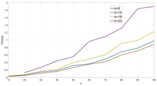
Figure 2. Calculation time with different dimensions when the diagonal number $k=9,13,19,23$.

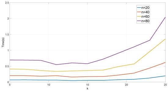
Figure 3. Calculation time with different diagonal numbers when the dimension $n=20,40,60,80$.

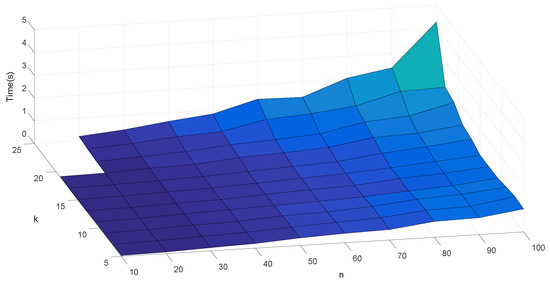
Figure 4. The variation of calculation time with different dimensions n and diagonal number k.

6. Conclusions

In this paper, a novel exact algorithm to the general linearly constrained zero-one quadratic programming problem with k-diagonal matrix is proposed. The algorithm is designed by analyzing the property of matrix Q and then combining the famous basic algorithm and dynamic programming method. The complexity of the algorithm is analyzed and shows that it is polynomially solvable when m is fixed. The experimental results also illustrate the feasibility and efficiency of the algorithm. Designing efficient algorithm to this special class of problem $01CQP$ not only provides useful information for designing efficient algorithms for other special classes but also can provide hints and facilitate the derivation of efficient relaxations for the general problems. And finally, the phasor measurement units placement problem is used to demonstrate that the algorithm has wide potential applications in decision-making real-life problems.

References

- Cook, W.J.; Cunningham, W.H.; Pulleyblank, W.R.; Schrijver, A. Combinatorial Optimization; Wiley-Interscience: Hoboken, NJ, USA, 1997. [Google Scholar]
- Hammer, P.L.; Rudeanu, S. Boolean Methods in Operations Research and Related Areas; Spring: Berlin/Heidelberg, Germany; New York, NY, USA, 1968. [Google Scholar]
- Chang, K.C.; Du, H.C. Efficient algorithms for layer assignment problem. IEEE Trans. Comput.-Aided Des. Integr. Circuits Syst. 1987, 6, 67–78. [Google Scholar] [CrossRef]
- Dehghan, A.; Mubarak, S. Binary quadratic programing for online tracking of hundreds of people in extremely crowded scenes. IEEE Trans. Pattern Anal. Mach. Intell. 2016, 40, 568–581. [Google Scholar] [CrossRef] [PubMed]
- Laughhunn, D.J. Quadratic binary programming with application to capital-budgeting problems. Oper. Res. 1970, 18, 454–461. [Google Scholar] [CrossRef]
- Kizys, R.; Juan, A.; Sawik, B.; Calvet, L. A biased-randomized iterated local search algorithm for rich portfolio optimization. Appl. Sci. 2019, 9, 3509. [Google Scholar] [CrossRef]
- Huang, L.; Zhang, Q.; Sun, L.; Sheng, Z. Robustness analysis of iterative learning control for a class of mobile robot systems with channel noise. IEEE Access 2019, 7, 34711–34718. [Google Scholar] [CrossRef]
- Manoli, G.; Rossi, M.; Pasetto, D.; Deiana, R.; Ferraris, S.; Cassiani, G.; Putti, M. An iterative particle filter approach for coupled hydro-geophysical inversion of a controlled infiltration experiment. J. Comput. Phys. 2015, 283, 37–51. [Google Scholar] [CrossRef]
- Mesbah, A. Stochastic model predictive control with active uncertainty learning: A Survey on dual control. Ann. Rev. Control 2018, 45, 107–117. [Google Scholar] [CrossRef]
- Imani, M.; Braga-Neto, U. Maximum-Likelihood adaptive filter for partially-observed boolean dynamical systems. IEEE Trans. Signal Process. 2017, 65, 359–371. [Google Scholar] [CrossRef]
- Imani, M.R.; Dougherty, E.; Braga-Neto, U. Boolean Kalman filter and smoother under model uncertainty. Automatica 2020, 111, 108609. [Google Scholar] [CrossRef]
- Baldwin, T.L.; Mili, L.; Boisen, M.B. Power system observability with minimal phasor measurement placement. IEEE Trans. Power Syst. 1993, 8, 707–715. [Google Scholar] [CrossRef]
- Nuqui, R.F.; Phadke, A.G. Phasor measurement unit placement techniques for complete and incomplete observability. IEEE Trans. Power Deliv. 2005, 20, 2381–2388. [Google Scholar] [CrossRef]
- Xu, B.; Abur, A. Observability analysis and measurement placement for system with PMUs. IEEE PES Power Syst. Conf. Expos. 2004, 2, 943–946. [Google Scholar]
- Gou, B. Generalized integer linear programming formulation for optimal PMU placement. IEEE Trans. Power Syst. 2008, 23, 1099–1104. [Google Scholar] [CrossRef]
- Kavasseri, R.; Srinivasan, S.K. Joint placement of phasor and power flow measurements for observability of power systems. IEEE Trans. Power Syst. 2011, 26, 1929–1936. [Google Scholar] [CrossRef]
- Poljak, S.; Rendl, F. Solving the max-cut problem using eigenvalues. Discret. Appl. Math. 1995, 62, 249–278. [Google Scholar] [CrossRef]
- Rendl, F.; Rinaldi, G.; Wiegele, A. Solving Max-Cut to optimality by intersecting semidefinite and polyhedral relaxations. Lect. Notes Comput. 2007, 4513, 295–309. [Google Scholar] [CrossRef]
- Ye, Y.A. 699-approximation algorithm for Max-Bisection. Math. Program. 2001, 90, 101–111. [Google Scholar] [CrossRef]
- Pardalos, P.M.; Rodgers, G.P. Computational aspects of a branch and bound algorithm for quadratic zero-one programming. Computing 1990, 45, 131–144. [Google Scholar] [CrossRef]
- Li, D.; Sun, X.L.; Liu, C.L. An exact solution method for unconstrained quadratic 0-1 programming: A geometric approach. J. Glob. Optim. 2012, 52, 797–829. [Google Scholar] [CrossRef]
- Gu, S.; Chen, X.Y.; Wang, L. Global optimization of binary quadratic programming: A neural network based algorithm and its FPGA Implementation. Neural Process. Lett. 2019, 1–20. [Google Scholar] [CrossRef]
- Zhu, W.X. Penalty parameter for linearly constrained 0-1 quadratic programming. J. Optim. Theory Appl. 2003, 116, 229–239. [Google Scholar] [CrossRef]
- Katayama, K.; Narihisa, H. Performance of simulated annealing-based heuristic for the unconstrained binary quadratic programming problem. Eur. J. Oper. Res. 2001, 134, 103–119. [Google Scholar] [CrossRef]
- Jiang, D.; Zhu, S. A method to solve nonintersection constraint 0-1 quadratic programming model. J. Southwest Jiaotong Univ. 1997, 32, 667–671. [Google Scholar]
- Ranjbar, M.; Effati, S.; Miri, S.M. An artificial neural network for solving quadratic zero-one programming problems. Neurocomputing 2017, 235, 192–198. [Google Scholar] [CrossRef]
- Ping, W.; Weiqing, X. Binary ant colony algorithm with controllable search bias for unconstrained binary quadratic problem. In Proceedings of the 2012 International Conference on Electronics, Communications and Control, Zhoushan, China, 16–18 October 2012. [Google Scholar]
- Gu, S.; Cui, R. Polynomial time solvable algorithm to linearly constrained binary quadratic programming problems with Q being a five-diagonal matrix. In Proceedings of the Fiveth International Conference on Intelligent Control and Information Processing, Dalian, China, 18–20 August 2014; pp. 366–372. [Google Scholar]
- Gu, S.; Cui, R.; Peng, J. Polynomial time solvable algorithms to a class of unconstrained and linearly constrained binary quadratic programming problems. Neurocomputing 2016, 198, 171–179. [Google Scholar] [CrossRef]
- Gu, S.; Peng, J.; Cui, R. A polynomial time solvable algorithm to binary quadratic programming problems with Q being a seven-diagonal matrix and its neural network implementation. In Proceedings of the ISNN 2014—Advances in Neural Networks, Macao, China, 28 November–1 December 2014; pp. 338–346. [Google Scholar]
- Gu, S.; Chen, X.Y. The basic algorithm for zero-one unconstrained quadratic programming problem with k-diagonal matrix. In Proceedings of the Twelfth International Conference on Advanced Computational Intelligence International, Dali, China, 14–16 March 2020. [Google Scholar]
© 2020 by the authors. Licensee MDPI, Basel, Switzerland. This article is an open access article distributed under the terms and conditions of the Creative Commons Attribution (CC BY) license (http://creativecommons.org/licenses/by/4.0/).