Bounded Perturbation Resilience and Superiorization of Proximal Scaled Gradient Algorithm with Multi-Parameters

Abstract

In this paper, a multi-parameter proximal scaled gradient algorithm with outer perturbations is presented in real Hilbert space. The strong convergence of the generated sequence is proved. The bounded perturbation resilience and the superiorized version of the original algorithm are also discussed. The validity and the comparison with the use or not of superiorization of the proposed algorithms were illustrated by solving the $l^1-l^2$ problem.

1. Introduction

The superiorization method, which was introduced by Censor in 2010 [1], can solve a broad class of nonlinear constrained optimal problems that result from many practical problems such as computed tomography [2], medical image recovery [3,4], convex feasibility problems [5,6], inverse problems of radiation therapy [7] and so on, which generates an automatic procedure based on the fact that the basic algorithm has the property of bounded perturbation resilience so that it is expected to get lower values of the objective function. In recent years, some researchers have focused on finding more applications of superiorization methodology while some other researchers have investigated the bounded perturbation resilience of algorithms—see, for examples, [8,9,10,11,12,13,14,15,16,17].

In this paper, we study the bounded perturbation resilience property and the corresponding superiorization of a proximal scaled gradient algorithm with multi-parameters for solving the following non-smooth composite optimization problem of the form

$$\underset{x\in H}{min}[f\left(x\right)+g\left(x\right)]=:\underset{x\in H}{min}\mathsf{\Phi }\left(x\right),$$

(1)

where H is a real Hilbert space endowed with an inner product $<·,·>$ and the induced norm $\Vert ·\Vert$. $f,g\in {\mathsf{\Gamma }}_0\left(H\right)$ with ${\mathsf{\Gamma }}_0\left(H\right)$ defined by

$${\mathsf{\Gamma }}_0\left(H\right):=\{f:H\to (-\infty ,+\infty ]|f\mathrm{is} \mathrm{proper} \mathrm{lower} \mathrm{semicontinuous} \mathrm{convex}\}.$$

In addition, f has L-Lipschitz continuous gredient $\nabla f$ on H with $L>0$.

The proximal gradient method is one of the popular iterative methods used for solving problem (1), which has received a lot of attention in the recent past due to its fast theoretical convergence rates and strong practical performance. Given an initial value $x_0\in H$, the proximal gradient method generates the following sequence $\left\{x_n\right\}$:

$$x_{n+1}=pro{x}_{\gamma g}(I-\gamma \nabla f)\left(x_n\right),\forall n\ge 0,$$

(2)

where $\gamma >0$ is the step size and $pro{x}_{\gamma g}$ is the proximal operator of g of order $\gamma$ (please refer to Definition 2, Section 2). Then, the generated sequence $\left\{x_n\right\}$ converges weakly to a solution of problem (1) if the solution set $S:=Argmin\left[f\right(x)+g(x\left)\right]\ne \varnothing$ and $0<\gamma <\frac{2}{L}$ (see, for instance, [18], Theorem 25.8).

Xu [19] raised the following more general proximal gradient algorithm:

$$x_{n+1}=pro{x}_{{\gamma }_{n}g}(I-{\gamma }_n\nabla f)\left(x_n\right).$$

(3)

The weak convergence of the generated sequence $\left\{x_n\right\}$ was obtained. If $dimH=\infty$, the strong convergence can not be guaranteed.

The scaled method was proposed by Strand [20] for increasing the rate of convergence of some algorithm. In a finite dimensional space, the selection of scaling matrices depends on the particular problem [21,22]. Jin, Censor and Jiang [13] introduced the following projected scaled gradient (PSG) algorithm:

$$x_{n+1}=P_C(I-{\gamma }_{n}D\nabla f)\left(x_n\right),\forall n\ge 0,$$

(4)

where $D\left(x_n\right)$ is a diagonal scaling matrix for each $x_n$, $P_C:{\mathbb{R}}^n\to C(\subset {\mathbb{R}}^n)$ is defined as $P_C\left(x\right)=inf\{\Vert x-y\Vert ,\forall y\in C\}$ for solving the following convex minimization problems:

$$\mathrm{minimize}J\left(x\right)\mathrm{subject} \mathrm{to}x\in C,$$

(5)

where $C\subset {\mathbb{R}}^n$ is a nonempty, closed and convex set, the objective function $J:C\to \mathbb{R}$ is convex. With the assumption that

$$\sum _{n=0}^{\infty }\Vert \nabla f\left(x_n\right)-D\left(x_n\right)\nabla f\left(x_n\right)\Vert <\infty$$

(6)

and other conditions, the convergence of the PSG method in the presence of bounded perturbations was proved.

Motivated by [13], Guo, Cui and Guo [23] discussed the proximal gradient algorithm with perturbations:

$$x_{n+1}=pro{x}_{{\lambda }_{n}g}(I-{\lambda }_{n}D\nabla f+e)x_n.$$

(7)

They proved that the generated sequence $\left\{x_n\right\}$ converges weakly to the solution of problem (1). After that, Guo and Cui [15] applied the convex combination of contraction operator and proximal gradient operator to obtain the strong convergence of the generated sequence and discussed the bounded perturbation resilience of the exact algorithm.

In this paper, we will study the following proximal scaled gradient algorithm with multi-parameters:

$$x_{n+1}:=t_{n}h\left(x_n\right)+{\gamma }_n{x}_n+{\lambda }_{n}pro{x}_{{\alpha }_{n}g}(x_n-{\alpha }_{n}D\left(x_n\right)\nabla f\left(x_n\right))+e_n,n\ge 0,$$

(8)

which is a further generalization of the above algorithms. We will discuss the strong convergence of (8) and the bounded perturbation resilience of its exact algorithm just like the algorithms named above. In addition, we also study the superiorized version of the exact algorithm of (8).

The rest is organized as follows. In the next section, we introduce some basic concepts and lemmas. In Section 3, we discuss the strong convergence results of the exact and non-exact algorithms. In Section 4, we provide two numerical examples for illustrating the performances of the iterations. Finally, we summarize the main points of this paper in Section 5.

2. Preliminaries

Let H be a real Hilbert space endowed by an inner product $<·,·>$ and the induced norm $\Vert ·\Vert$. Let $\left\{x_n\right\}$ be a sequence in H. $z\in H$ is said to be a weak cluster point of $\left\{x_n\right\}$ if there exists a subsequence $\left\{x_{n_j}\right\}$ of $\left\{x_n\right\}$ that converges weakly to it. The set of all weak cluster points of $\left\{x_n\right\}$ is denoted by ${\omega }_w\left(x_n\right)$. Let $T:H\to H$ be a nonlinear operator. Set $Fix\left(T\right):=\{x\in H:Tx=x\}$.

The following definitions are needed in proving our main results.

Definition 1.

([24], Proposition 2.1)

(i)

T is non-expansive if

$$\Vert Tx-Ty\Vert \le \Vert x-y\Vert ,\forall x,y\in H.$$

(9)

(ii)

T is L-Lipschitz continuous with $L\ge 0$, if

$$\Vert Tx-Ty\Vert \le L\Vert x-y\Vert ,\forall x,y\in H.$$

(10)

We call T a contractive mapping if $0\le L<1$.

(iii)

T is firmly non-expansive if

$${\Vert Tx-Ty\Vert }^2\le {\Vert x-y\Vert }^2-{\Vert (I-T)x-(I-T)y\Vert }^2.$$

(11)

(iv)

T is α-averaged if there exists a non-expansive operator $S:H\to H$ and $\alpha \in (0,1)$, such that

$$T=(1-\alpha )I+\alpha S.$$

(12)

In particular, a firmly non-expansive mapping is $\frac{1}{2}$-averaged.

(v)

T is v-inverse strongly monotone (v-ism) with $v>0$, if

$$⟨Tx-Ty,x-y⟩\ge {v\Vert Tx-Ty\Vert }^2,\forall x,y\in H.$$

(13)

Definition 2.

([25], Proximal Operator) Let $g\in {\mathsf{\Gamma }}_0\left(H\right)$. The proximal operator of g is defined by

$$pro{x}_g\left(x\right):=arg\underset{y\in H}{min}\{\frac{{\Vert y-x\Vert }^2}{2}+g\left(y\right)\},x\in H.$$

(14)

The above definition is well defined since $\frac{{\Vert y-x\Vert }^2}{2}+g\left(y\right)$ has only one minimizer on H for each $x\in H$ and for given $g\in {\mathsf{\Gamma }}_0\left(H\right)$ (see [18], Proposition 12.15).

The proximal operator of g of order $\alpha >0$ is defined as

$$pro{x}_{\alpha g}\left(x\right):=arg\underset{y\in H}{min}\{\frac{{\Vert y-x\Vert }^2}{2\alpha }+g\left(y\right)\},x\in H.$$

(15)

The following Lemmas 1–3 describe the properties of proximal operators.

Lemma 1.

([19,26], Lemma 2.4, Lemma 3.3) Let $g\in {\mathsf{\Gamma }}_0\left(H\right)$, and $\alpha >0,\mu >0$. Then,

$$pro{x}_{\alpha g}\left(x\right)=pro{x}_{\mu g}(\frac{\mu }{\alpha }x+(1-\frac{\mu }{\alpha })pro{x}_{\alpha g}x).$$

(16)

Moreover, if $\alpha <\mu$, we also have

$$\Vert x-pro{x}_{\alpha g}(I-\alpha \nabla f)x\Vert \le 2\Vert x-pro{x}_{\mu g}(I-\mu \nabla f)x\Vert ,\forall x\in H.$$

(17)

Lemma 2.

[18] (Non-expansiveness) Let $g\in {\mathsf{\Gamma }}_0\left(H\right)$ and $\alpha >0$. Then, the proximal operator $pro{x}_{\alpha g}$ is $\frac{1}{2}$-averaged. We obtain the non-expansiveness of the proximal operator

$$\Vert pro{x}_{\alpha g}\left(x\right)-pro{x}_{\alpha g}\left(y\right)\Vert \le \Vert x-y\Vert ,\forall x,y\in H.$$

(18)

Lemma 3.

([19], Propostion 3.2) Let $f,g\in {\mathsf{\Gamma }}_0\left(H\right)$, f be differentiable and $z\in H,\alpha >0$. Then, z is a solution to (1) if and only if z is the fixed point of the following equation:

$$z=pro{x}_{\alpha g}(I-\alpha \nabla f)z.$$

(19)

The following lemmas play important roles in proving the strong convergence result.

Lemma 4.

([18], Corollary 4.18) Let $T:H\to H$ be a non-expansive mapping with $Fix\left(T\right)\ne \varnothing$. If $\left\{x_n\right\}$ is a sequence in H converging weakly to x and if $\left\{(I-T)x_n\right\}$ converges strongly to 0, then $(I-T)x=0$.

Lemma 5.

([27], Lemma 2.5) Assume that $\left\{s_n\right\}$ is a sequence of nonnegative real numbers satisfying

$$s_{n+1}\le (1-{\gamma }_n)s_n+{\gamma }_n{\delta }_n+{\beta }_n,n\ge 0,$$

(20)

where $\left\{{\gamma }_n\right\}\subset [0,1]$, $\left\{{\delta }_n\right\}\subset \mathbb{R}$ such that

(i)

${\sum }_{n=0}^{\infty }{\gamma }_n=\infty$;

(ii)

$lim{sup}_{n\to \infty }{\delta }_n\le 0$;

(iii)

${\sum }_{n=0}^{\infty }{\beta }_n<\infty$.

Then, ${lim}_{n\to \infty }{s}_n=0$.

Lemma 6.

([28], Lemma 2.4) Let $x,y\in H$ and $\alpha ,\beta \in \mathbb{R}$. Then,

(i)

${\Vert x+y\Vert }^2\le {\Vert x\Vert }^2+2⟨y,x+y⟩$;

(ii)

${\Vert \alpha x+\beta y\Vert }^2={\alpha (\alpha +\beta )\Vert x\Vert }^2+{\beta (\alpha +\beta )\Vert y\Vert }^2-\alpha \beta {\Vert x-y\Vert }^2$;

(iii)

${\Vert \alpha x+(1-\alpha )y\Vert }^2={\alpha \Vert x\Vert }^2+{(1-\alpha )\Vert y\Vert }^2-\alpha (1-\alpha ){\Vert x-y\Vert }^2$.

Lemma 7.

([23], Proposition 3.3) Let $f,g\in {\mathsf{\Gamma }}_0\left(H\right)$. For any $0<\alpha <\frac{2}{L}$, where L is the Lipschitz constant of $\nabla f$. $pro{x}_{\alpha g}(I-\alpha \nabla f)$ is $\frac{\alpha L+2}{4}$-averaged. Hence, it is non-expansive.

3. The Convergence Analysis and the Superiorized Version

In this section, we prove that the sequence $\left\{v_n\right\}$ generated by the exact form of (8) converges strongly to a solution of problem (1) at first. Then, we discuss the strong convergence of algorithm (8). Finally, we investigate the bounded perturbation resilience of the exact iteration by viewing it as a special case of algorithm (8). The superiorized version is also presented at the end of this section.

3.1. The Exact Form of Algorithm (8)

Given the errors $e_n\equiv 0,n\ge 0$ in (8), we get the exact version of (8):

$$\begin{array}{cc}{v}_{n+1}\hfill & =t_{n}h\left(v_n\right)+{\gamma }_n{v}_n+{\lambda }_{n}pro{x}_{{\alpha }_{n}g}(v_n-{\alpha }_{n}D\left(v_n\right)\nabla f\left(v_n\right))\hfill \\ & =:t_{n}h\left(v_n\right)+{\gamma }_n{v}_n+{\lambda }_{n}pro{x}_{{\alpha }_{n}g}(I-{\alpha }_{n}D\nabla f)v_n,\hfill \end{array}$$

(21)

where $\left\{t_n\right\}$, $\left\{{\gamma }_n\right\},\left\{{\lambda }_n\right\}\subset [0,1]$ such that $0<{inf}_n{\gamma }_n$ and $t_n+{\gamma }_n+{\lambda }_n=1$ for all $n\ge 0$. $h:H\to H$ is a $\rho$-contraction for some $\rho \in [0,1)$. $f,g\in {\mathsf{\Gamma }}_0\left(H\right)$, f has the Lipschitz continuous gradient $\nabla f$ with Lipschitz constant $L>0$. $D\left(x\right):H\to H$ is a linear bounded operator for each $x\in H$ with an upper bound $N_x$ and satisfies

$$\sum _{n=0}^{\infty }\Vert \nabla f\left(v_n\right)-D\left(v_n\right)\nabla f\left(v_n\right)\Vert =:\sum _{n=0}^{\infty }\Vert \theta \left(v_n\right)\Vert <\infty .$$

(22)

Provided that $\left\{t_n\right\},\left\{{\lambda }_n\right\}$ and $\left\{{\alpha }_n\right\}$ satisfy some additional conditions, we get the following strong convergence result of algorithm (21).

Theorem 1.

Suppose that the solution set S of (1) is not empty, (22) and the following conditions hold:

(i)

$0<\alpha :={inf}_n{\alpha }_n\le {\alpha }_n<\frac{2}{L}$ for all n;

(ii)

${lim}_{n\to \infty }{t}_n=0$ and ${\sum }_{n=0}^{\infty }{t}_n=\infty$;

(iii)

${lim}_{n\to \infty }\frac{t_n}{{\lambda }_n}=0$.

The sequence $\left\{v_n\right\}$ generated by algorithm (21) converges strongly to a point $z\in S$, where z is the unique solution of the following variational inequality problem:

$$⟨(I-h)z,v-z⟩\ge 0,v\in S.$$

(23)

Proof of Theorem 1.

We will complete the proof by three steps.

Step 1.$\left\{v_n\right\}$ is a bounded sequence in H.

Let $z\in S$, then we have $z=pro{x}_{{\alpha }_{n}g}(I-{\alpha }_n\nabla f)z$ by Lemma 3. In view of Lemmas 2 and 7, we also get that $pro{x}_{{\alpha }_{n}g}$ and $pro{x}_{{\alpha }_{n}g}(I-{\alpha }_n\nabla f)$ are non-expansive for $n\ge 0$. Now, let us calculate

$$\begin{array}{c}\Vert v_{n+1}-z\Vert \hfill \\ =\Vert t_n(h\left(v_n\right)-z)+{\gamma }_n(v_n-z)+{\lambda }_n(pro{x}_{{\alpha }_{n}g}(I-{\alpha }_{n}D\nabla f)v_n-z)\Vert \hfill \\ \le t_n\Vert h\left(v_n\right)-h\left(z\right)+h\left(z\right)-z\Vert +{\gamma }_n\Vert v_n-z\Vert \hfill \\ +{\lambda }_n\Vert pro{x}_{{\alpha }_{n}g}(I-{\alpha }_{n}D\nabla f)v_n-pro{x}_{{\alpha }_{n}g}(I-{\alpha }_n\nabla f)z\Vert \hfill \\ \le t_n\rho \Vert v_n-z\Vert +t_n\Vert h\left(z\right)-z\Vert +{\gamma }_n\Vert v_n-z\Vert \hfill \\ +{\lambda }_n\Vert pro{x}_{{\alpha }_{n}g}(I-{\alpha }_{n}D\nabla f)v_n-pro{x}_{{\alpha }_{n}g}(I-{\alpha }_n\nabla f)v_n\hfill \\ +pro{x}_{{\alpha }_{n}g}(I-{\alpha }_n\nabla f)v_n-pro{x}_{{\alpha }_{n}g}(I-{\alpha }_n\nabla f)z\Vert \hfill \\ \le (1-t_n(1-\rho ))\Vert v_n-z\Vert +t_n\Vert h\left(z\right)-z\Vert +{\lambda }_n{\alpha }_n\Vert \theta \left(v_n\right)\Vert \hfill \\ =(1-t_n(1-\rho ))\Vert v_n-z\Vert +t_n(1-\rho )\frac{1}{(1-\rho )}\Vert h\left(z\right)-z\Vert \hfill \\ +(1-t_n-{\gamma }_n){\alpha }_n\Vert \theta \left(v_n\right)\Vert \hfill \\ \le (1-t_n(1-\rho ))\Vert v_n-z\Vert +t_n(1-\rho )\frac{1}{(1-\rho )}\Vert h\left(z\right)-z\Vert \hfill \\ +(1-t_n+t_n\rho ){\alpha }_n\Vert \theta \left(v_n\right)\Vert \hfill \\ =(1-t_n(1-\rho ))(\Vert v_n-z\Vert +{\alpha }_n\Vert \theta \left(v_n\right)\Vert )+t_n(1-\rho )\frac{1}{(1-\rho )}\Vert h\left(z\right)-z\Vert \hfill \\ \le max\{\Vert v_n-z\Vert +{\alpha }_n\Vert \theta \left(v_n\right)\Vert ,\frac{\Vert h\left(z\right)-z\Vert }{1-\rho }\}.\hfill \end{array}$$

(24)

An induction argument shows that

$$\begin{array}{cc}\Vert v_{n+1}-z\Vert \hfill & \le max\{\Vert v_0-z\Vert +{\sum }_{k=0}^n{\alpha }_k\Vert \theta \left(v_k\right)\Vert ,\frac{\Vert h\left(z\right)-z\Vert }{1-\rho }\}\hfill \\ & \le max\{\Vert v_0-z\Vert +M,\frac{\Vert h\left(z\right)-z\Vert }{1-\rho }\},\hfill \end{array}$$

(25)

where $M:={\sum }_{n=0}^{\infty }{\alpha }_n\Vert \theta \left(v_n\right)\Vert <\infty$ as $\left\{{\alpha }_n\right\}$ is bounded and ${\sum }_{n=0}^{\infty }\Vert \theta \left(v_n\right)\Vert <\infty$. Hence, $\left\{v_n\right\}$ is bounded. Consequently, $\left\{h\left(v_n\right)\right\}$ is bounded since h is a $\rho$-contraction.

Step 2. There exists a subsequence $\left\{v_{n_j}\right\}\subset \left\{v_n\right\}$ such that ${\omega }_w\left(v_{n_j}\right)\subset S$.

We denote by

$$\begin{array}{c}{D}_n:=pro{x}_{{\alpha }_{n}g}(I-{\alpha }_{n}D\nabla f),\hfill \\ T_n:=pro{x}_{{\alpha }_{n}g}(I-{\alpha }_n\nabla f)\hfill \end{array}$$

(26)

for briefness.

Using the notation ${\rho }_n:=\frac{{\lambda }_n}{1-t_n}$, one has ${\rho }_n\in (0,1)$,

$$\begin{array}{cc}\hfill u_n:& =\frac{1}{1-t_n}({\gamma }_n{v}_n+{\lambda }_{n}pro{x}_{{\alpha }_{n}g}(I-{\alpha }_{n}D\nabla f)v_n)\hfill \\ & =(1-{\rho }_n)v_n+{\rho }_n{D}_n{v}_n,\hfill \\ \hfill v_{n+1}:& =t_{n}h\left(v_n\right)+(1-t_n)u_n.\hfill \end{array}$$

(27)

Given $z\in S$, we consider by utilizing Lemma 6 (iii)

$$\begin{array}{c}\Vert v_{n+1}{-z\Vert }^2\hfill \\ =\Vert t_n(h\left(v_n\right)-z)+(1-t_n)(u_n-z){\Vert }^2\hfill \\ =\Vert t_n(h\left(v_n\right)-h\left(z\right)+h\left(z\right)-z)+(1-t_n)(u_n-z){\Vert }^2\hfill \\ \le \Vert t_n(h\left(v_n\right)-h\left(z\right))+(1-t_n)(u_n-z){\Vert }^2+2t_n⟨h\left(z\right)-z,v_{n+1}-z⟩\hfill \\ \le t_n{\rho }^2\Vert v_n{-z\Vert }^2+(1-t_n){\Vert u_n-z\Vert }^2+2t_n⟨h\left(z\right)-z,v_{n+1}-z⟩.\hfill \end{array}$$

(28)

Meanwhile, we derive

$$\begin{array}{c}\Vert u_n{-z\Vert }^2\hfill \\ =\Vert (1-{\rho }_n)v_n+{\rho }_n{D}_n{v}_n{-z\Vert }^2\hfill \\ =\Vert v_n-z+{\rho }_n(D_n{v}_n-v_n){\Vert }^2\hfill \\ =\Vert v_n{-z\Vert }^2+{\rho }_n^2{\Vert D_n{v}_n-v_n\Vert }^2-2{\rho }_n⟨v_n-z,v_n-D_n{v}_n⟩\hfill \\ =\Vert v_n{-z\Vert }^2+{\rho }_n^2\Vert D_n{v}_n-v_n{\Vert }^2-{\rho }_n(\Vert v_n{-z\Vert }^2+\Vert D_n{v}_n-v_n{\Vert }^2-\Vert D_n{v}_n-z{\Vert }^2)\hfill \\ =(1-{\rho }_n)\Vert v_n{-z\Vert }^2-{\rho }_n(1-{\rho }_n)\Vert D_n{v}_n-v_n{\Vert }^2+{\rho }_n{\Vert D_n{v}_n-z\Vert }^2.\hfill \end{array}$$

(29)

Notice that

$$\begin{array}{c}\Vert D_n{v}_n-v_n{\Vert }^2\hfill \\ =\Vert (D_n-T_n)v_n+T_n{v}_n-v_n{\Vert }^2\hfill \\ \le {\alpha }_n^2\Vert \theta \left(v_n\right){\Vert }^2+\Vert T_n{v}_n-v_n{\Vert }^2+2{\alpha }_n\Vert \theta \left(v_n\right)\Vert \Vert T_n{v}_n-v_n\Vert ,\hfill \end{array}$$

(30)

and that

$$\begin{array}{c}\Vert D_n{v}_n{-z\Vert }^2\hfill \\ =\Vert D_n{v}_n-T_n{v}_n+T_n{v}_n{-z\Vert }^2\hfill \\ \le {\alpha }_n^2\Vert \theta \left(v_n\right){\Vert }^2+\Vert v_n{-z\Vert }^2+2{\alpha }_n\Vert \theta \left(v_n\right)\Vert \Vert T_n{v}_n-z\Vert \hfill \\ \le {\alpha }_n^2\Vert \theta \left(v_n\right){\Vert }^2+\Vert v_n{-z\Vert }^2+2{\alpha }_n\Vert \theta \left(v_n\right)\Vert \Vert v_n-z\Vert \hfill \end{array}$$

(31)

since $T_n$ is non-expansive and $z=T_{n}z$ (see Lemma 3). We then obtain by substituting (30) and (31) into (29)

$$\begin{array}{c}\Vert u_n{-z\Vert }^2\hfill \\ =(1-{\rho }_n)\Vert v_n{-z\Vert }^2-{\rho }_n(1-{\rho }_n)\Vert D_n{v}_n-v_n{\Vert }^2+{\rho }_n{\Vert D_n{v}_n-z\Vert }^2\hfill \\ \le (1-{\rho }_n){\Vert v_n-z\Vert }^2\hfill \\ -{\rho }_n(1-{\rho }_n)\left({\alpha }_n^2\Vert \theta \left(v_n\right){\Vert }^2+\Vert T_n{v}_n-v_n{\Vert }^2+2{\alpha }_n\Vert \theta \left(v_n\right)\Vert \Vert T_n{v}_n-v_n\Vert \right)\hfill \\ +{\rho }_n\left({\alpha }_n^2\Vert \theta \left(v_n\right){\Vert }^2+\Vert v_n{-z\Vert }^2+2{\alpha }_n\Vert \theta \left(v_n\right)\Vert \Vert v_n-z\Vert \right)\hfill \\ =\Vert v_n{-z\Vert }^2-{\rho }_n(1-{\rho }_n)\Vert T_n{v}_n-v_n{\Vert }^2+{\rho }_n^2{\alpha }_n^2{\Vert \theta \left(v_n\right)\Vert }^2\hfill \\ -2{\alpha }_n{\rho }_n(1-{\rho }_n)\Vert \theta \left(v_n\right)\Vert \Vert T_n{v}_n-v_n\Vert +2{\rho }_n{\alpha }_n\Vert \theta \left(v_n\right)\Vert \Vert v_n-z\Vert .\hfill \end{array}$$

(32)

Combining (28) and (32), we get

$$\begin{array}{c}\Vert v_{n+1}{-z\Vert }^2\hfill \\ \le t_n{\rho }^2\Vert v_n{-z\Vert }^2+(1-t_n){\Vert u_n-z\Vert }^2+2t_n⟨h\left(z\right)-z,v_{n+1}-z⟩\hfill \\ \le t_n{\rho }^2\Vert v_n{-z\Vert }^2+(1-t_n)[\Vert v_n{-z\Vert }^2-{\rho }_n(1-{\rho }_n)\Vert T_n{v}_n-v_n{\Vert }^2+{\rho }_n^2{\alpha }_n^2{\Vert \theta \left(v_n\right)\Vert }^2\hfill \\ -2{\alpha }_n{\rho }_n(1-{\rho }_n)\Vert \theta \left(v_n\right)\Vert \Vert T_n{v}_n-v_n\Vert +2{\rho }_n{\alpha }_n\Vert \theta \left(v_n\right)\Vert \Vert v_n-z\Vert ]\hfill \\ +2t_n⟨h\left(z\right)-z,v_{n+1}-z⟩\hfill \\ =(t_n{\rho }^2+(1-t_n))\Vert v_n{-z\Vert }^2-{\rho }_n(1-{\rho }_n)(1-t_n){\Vert T_n{v}_n-v_n\Vert }^2\hfill \\ +{\rho }_n^2(1-t_n){\alpha }_n^2\Vert \theta \left(v_n\right){\Vert }^2-2{\alpha }_n{\lambda }_n(1-{\rho }_n)\Vert \theta \left(v_n\right)\Vert \Vert T_n{v}_n-v_n\Vert \hfill \\ +2{\lambda }_n{\alpha }_n\Vert \theta \left(v_n\right)\Vert \Vert v_n-z\Vert +2t_n⟨h\left(z\right)-z,v_{n+1}-z⟩\hfill \\ \le (1-t_n(1-{\rho }^2))\Vert v_n{-z\Vert }^2-{\lambda }_n(1-{\rho }_n){\Vert T_n{v}_n-v_n\Vert }^2\hfill \\ +{\rho }_n^2(1-t_n){\alpha }_n^2\Vert \theta \left(v_n\right){\Vert }^2+2{\lambda }_n{\alpha }_n\Vert \theta \left(v_n\right)\Vert \Vert v_n-z\Vert +2t_n⟨h\left(z\right)-z,v_{n+1}-z⟩\hfill \\ =(1-{\overline{t}}_n)\Vert v_n{-z\Vert }^2+{\rho }_n{\lambda }_n{\alpha }_n^2\Vert \theta \left(v_n\right){\Vert }^2+2{\lambda }_n{\alpha }_n\Vert \theta \left(v_n\right)\Vert \Vert v_n-z\Vert \hfill \\ +{\overline{t}}_n\left[\frac{2}{1-{\rho }^2}⟨h\left(z\right)-z,v_{n+1}-z⟩-\frac{{\lambda }_n{\gamma }_n}{t_n(1-t_n)(1-{\rho }^2)}{\Vert T_n{v}_n-v_n\Vert }^2\right]\hfill \\ \le (1-{\overline{t}}_n){\Vert v_n-z\Vert }^2+{\overline{t}}_n{\zeta }_n+U_n,\hfill \end{array}$$

(33)

where ${\overline{t}}_n:=t_n(1-{\rho }^2)$,

$$\begin{array}{c}{\zeta }_n:=\frac{2}{1-{\rho }^2}⟨h\left(z\right)-z,v_{n+1}-z⟩-\frac{{\lambda }_n{\gamma }_n}{t_n(1-t_n)(1-{\rho }^2)}{\Vert T_n{v}_n-v_n\Vert }^2,\hfill \\ U_n:={\rho }_n{\lambda }_n{\alpha }_n^2\Vert \theta \left(v_n\right){\Vert }^2+2{\lambda }_n{\alpha }_n\Vert \theta \left(v_n\right)\Vert \Vert v_n-z\Vert .\hfill \end{array}$$

(34)

Obviously, we have

$$\begin{array}{c}\hfill |{\zeta }_n|\le \frac{1}{1-{\rho }^2}\Vert h\left(z\right)-z\Vert \Vert v_n-z\Vert <\infty ,\end{array}$$

(35)

which implies that $lim{sup}_{n\to \infty }{\zeta }_n$ is a finite number. Thus, there exists a subsequence $\left\{{\zeta }_{n_j}\right\}\subset \left\{{\zeta }_n\right\}$ such that $lim{sup}_{n\to \infty }{\zeta }_n={lim}_{j\to \infty }{\zeta }_{n_j}$. In addition, without loss of generality, we may assume that $v_{n_j}$ converges weakly to some $v^{*}\in H$ as $j\to \infty$ since $\left\{v_n\right\}$ is bounded. Notice that

$$\begin{array}{c}\Vert v_{n_j+1}-v_{n_j}\Vert =\Vert t_{n_j}(h\left(v_{n_j}\right)-v_{n_j})+{\lambda }_{n_j}(D_{n_j}{v}_{n_j}-v_{n_j})\Vert \hfill \\ \le t_{n_j}\Vert h\left(v_{n_j}\right)-v_{n_j}\Vert +{\lambda }_{n_j}\Vert D_{n_j}{v}_{n_j}-T_{n_j}{v}_{n_j}+T_{n_j}{v}_{n_j}-v_{n_j}\Vert \hfill \\ \le t_{n_j}[\Vert h\left(v_{n_j}\right)\Vert +\Vert v_{n_j}\Vert ]+{\lambda }_{n_j}{\alpha }_{n_j}\Vert \theta \left(v_{n_j}\right)\Vert +{\lambda }_{n_j}\Vert T_{n_j}{v}_{n_j}-v_{n_j}\Vert \hfill \\ \to 0,asj\to \infty .\hfill \end{array}$$

(36)

We conclude that $\left\{v_{n_j+1}\right\}$ also converges weakly to $v^{*}$. As a result, ${lim}_{n\to \infty }⟨h\left(z\right)-z,v_{n_j+1}-z⟩$ exists. Hence, we have

$$\begin{array}{c}lim{sup}_{n\to \infty }{\zeta }_n={lim}_{j\to \infty }{\zeta }_{n_j}\hfill \\ ={lim}_{j\to \infty }\left[\frac{1}{1-{\rho }^2}⟨h\left(z\right)-z,v_{n_j+1}-z⟩-\frac{{\lambda }_{n_j}{\gamma }_{n_j}}{t_{n_j}(1-t_{n_j})(1-{\rho }^2)}{\Vert T_{n_j}{v}_{n_j}-v_{n_j}\Vert }^2\right]\hfill \\ =\frac{1}{1-{\rho }^2}⟨h\left(z\right)-z,v^{*}-z⟩-{lim}_{j\to \infty }\frac{{\lambda }_{n_j}{\gamma }_{n_j}}{t_{n_j}(1-t_{n_j})(1-{\rho }^2)}{\Vert T_{n_j}{v}_{n_j}-v_{n_j}\Vert }^2.\hfill \end{array}$$

(37)

In light of the fact that $\{\frac{{\gamma }_{n_j}}{1-t_{n_j}}\}$ is bounded and ${inf}_n\frac{{\gamma }_{n_j}}{1-t_{n_j}}>0$, the sequence $\{\frac{{\lambda }_{n_j}}{t_{n_j}}\Vert T_{n_j}{v}_{n_j}-v_{n_j}{\Vert }^2\}$ is bounded. Then, condition (iii) implies

$$\begin{array}{c}{lim}_{j\to \infty }\Vert T_{n_j}{v}_{n_j}-v_{n_j}\Vert =0.\hfill \end{array}$$

(38)

Set $T:=pro{x}_{\alpha g}(I-\alpha \nabla f)$ with $\alpha ={inf}_n{\alpha }_n>0$ and apply Lemma 1. We get

$$\begin{array}{c}\hfill \underset{j\to \infty }{lim}\Vert T{v}_{n_j}-v_{n_j}\Vert \le 2\underset{j\to \infty }{lim}\Vert T_{n_j}{v}_{n_j}-v_{n_j}\Vert =0.\end{array}$$

(39)

Then, Lemma 4 guarantees that ${\omega }_w\left(v_{n_j}\right)\subset S$.

Step 3.$\left\{v_n\right\}$ converges strongly to $z\in S$.

Let us show that (33) satisfies the conditions of Lemma 5. From Step 2, it has $v_{n_j+1}\rightharpoonup v^{*}(\in S)$ as $j\to \infty$. Therefore,

$$\begin{array}{cc}{lim\; sup}_{n\to \infty }{\zeta }_n\hfill & \le \frac{2}{1-{\rho }^2}{lim\; sup}_{n\to \infty }⟨h\left(z\right)-z,v_{n+1}-z⟩\hfill \\ & =\frac{2}{1-{\rho }^2}{lim}_{j\to \infty }⟨h\left(z\right)-z,v_{n_j+1}-z⟩\hfill \\ & =\frac{2}{1-{\rho }^2}⟨h\left(z\right)-z,v^{*}-z⟩\hfill \\ & \le 0.\hfill \end{array}$$

(40)

In addition, it is obvious that ${\sum }_{n=0}^{\infty }{U}_n<\infty$ (see (34)) since $\left\{{\rho }_n\right\},\left\{{\lambda }_n\right\},\left\{{\alpha }_n\right\}$, $\{\Vert v_n-z\Vert \}$ are bounded sequences and ${\sum }_{n=0}^{\infty }\Vert \theta \left(v_n\right)\Vert <\infty$. Finally, we apply Lemma 5 to (33) to conclude that $\Vert v_n-z\Vert \to 0$, as $n\to \infty$. This ends the proof. □

3.2. The Strong Convergence of Algorithm (8)

Theorem 2.

Suppose that the solution set S of (1) is not empty, (22) and the following conditions hold:

(i)

$0<\alpha :={inf}_n{\alpha }_n\le {\alpha }_n<\frac{2}{L}$ for all n;

(ii)

${lim}_{n\to \infty }{t}_n=0$ and ${\sum }_{n=0}^{\infty }{t}_n=\infty$;

(iii)

${lim}_{n\to \infty }\frac{t_n}{{\lambda }_n}=0$;

(iv)

${\sum }_{n=0}^{\infty }\Vert e_n\Vert <\infty$.

Then, the sequence $\left\{x_n\right\}$ generated by algorithms (8) converges strongly to a point $z\in S$.

Proof of Theorem 2.

Let $\left\{x_n\right\},\left\{v_n\right\}$ be generated by (8) and (21), respectively. Then, $\left\{v_n\right\}$ converges strongly to a solution of problem (1) according to Theorem 1. Thus, we only need to prove that $\Vert x_n-v_n\Vert \to 0$ as $n\to \infty$.

We denote by $D_n:=pro{x}_{{\alpha }_{n}g}(I-{\alpha }_{n}D\nabla f)$ and $T_n:=pro{x}_{{\alpha }_{n}g}(I-{\alpha }_n\nabla f)$, respectively. $T_n$ is non-expansive according to Lemma 7. Then, we have

$$\begin{array}{c}\Vert x_{n+1}-v_{n+1}\Vert \hfill \\ =\Vert t_n(h\left(x_n\right)-h\left(v_n\right))+{\gamma }_n(x_n-v_n)+{\lambda }_n[pro{x}_{{\alpha }_{n}g}(I-{\alpha }_{n}D\nabla f)x_n\hfill \\ -pro{x}_{{\alpha }_{n}g}(I-{\alpha }_{n}D\nabla f)v_n]+e_n\Vert \hfill \\ =\Vert t_n(h\left(x_n\right)-h\left(v_n\right))+{\gamma }_n(x_n-v_n)+{\lambda }_n((D_n-T_n)\left(x_n\right)-(D_n-T_n)\left(v_n\right)\hfill \\ +T_n\left(x_n\right)-T_n\left(v_n\right))+e_n\Vert \hfill \\ \le t_n\Vert h\left(x_n\right)-h\left(v_n\right)\Vert +{\gamma }_n\Vert x_n-v_n\Vert +{\lambda }_n(\Vert (D_n-T_n)\left(x_n\right)\Vert +\Vert (D_n-T_n)\left(v_n\right)\Vert \hfill \\ +\Vert T_n\left(x_n\right)-T_n\left(v_n\right)\Vert )+\Vert e_n\Vert \hfill \\ \le t_n\rho \Vert x_n-v_n\Vert +{\gamma }_n\Vert x_n-v_n\Vert +{\lambda }_n[{\alpha }_n(\Vert \theta \left(x_n\right)\Vert +\Vert \theta \left(v_n\right)\Vert )+\Vert x_n-v_n\Vert ]+\Vert e_n\Vert \hfill \\ \le (1-t_n(1-\rho ))\Vert x_n-v_n\Vert +{\lambda }_n{\alpha }_n(\Vert \theta \left(x_n\right)\Vert +\Vert \theta \left(v_n\right)\Vert )+\Vert e_n\Vert .\hfill \end{array}$$

(41)

Applying Lemma 5 to inequality (41), we get $\Vert x_n-v_n\Vert \to 0$ as $n\to \infty$. We then have completed the proof owing to Theorem 1. □

3.3. Bounded Perturbation Resilience

This subsection is devoted to verifying the bounded perturbation resilience property of algorithm (21) and showing the superiorized version of it.

Given a problem $\mathsf{\Psi }$, let $A:H\to H$ be a basic algorithm operator.

Definition 3.

[9] An algorithmic operator A is bounded perturbation resilient if the sequence $\left\{v_n\right\}$, generated by $v_{n+1}=A{v}_n$ with $v_0\in H$, converges to a solution to Ψ; then, any sequence $\left\{x_n\right\}$ generated by $x_{n+1}=A(x_n+{\beta }_n{y}_n)$ with any $x_0\in H$, also converges to a solution of Ψ, where ${\left\{y_n\right\}}_{n=0}^{\infty }\subset H$ is bounded, and ${\left\{{\beta }_n\right\}}_{n=0}^{\infty }\subset \mathbb{R}$ are such that ${\beta }_n\ge 0$ for all $n\ge 0$ and ${\sum }_{n=0}^{\infty }{\beta }_n<\infty$.

If we take algorithm (21) as the basic algorithm A, the following iteration is the bounded perturbation of it:

$$x_{n+1}:=t_{n}h(x_n+{\beta }_n{y}_n)+{\gamma }_n(x_n+{\beta }_n{y}_n)+{\lambda }_{n}pro{x}_{{\alpha }_{n}g}(I-{\alpha }_{n}D\nabla f)(x_n+{\beta }_n{y}_n),n\ge 0.$$

(42)

We have the following result.

Theorem 3.

Let H be a real Hilbert space, and $h:H\to H$ a ρ-contractive operator with $\rho \in (0,1)$, f, $g\in {\mathsf{\Gamma }}_0\left(H\right)$. Assume that the solution set S to (1) is nonempty and that f has Lipschitz continuous gradient $\nabla f$ on H with the Lipschitz constant $L>0$. $\left\{{\beta }_n\right\}$, $\left\{y_n\right\}$ satisfy the conditions in Definition 3, $\left\{t_n\right\}$, $\left\{{\gamma }_n\right\}$, $\left\{{\lambda }_n\right\}$ and $\left\{{\alpha }_n\right\}$ satisfy the conditions in Theorem 1, respectively. Then, any sequence $\left\{x_n\right\}$ generated by (42) converges strongly to a point $x^{*}$ in S. Thus, algorithm (21) is bounded perturbation resilient.

Proof of Theorem 3.

We can rewrite algorithm (42) as

$$x_{n+1}=t_{n}h\left(x_n\right)+{\gamma }_n{x}_n+{\lambda }_{n}pro{x}_{{\alpha }_{n}g}(I-{\alpha }_{n}D\nabla f)x_n+{\tilde{e}}_n$$

(43)

with

$$\begin{array}{c}{\tilde{e}}_n:=t_n(h(x_n+{\beta }_n{y}_n)-h\left(x_n\right))+{\gamma }_n{\beta }_n{y}_n\hfill \\ +{\lambda }_n[pro{x}_{{\alpha }_{n}g}(I-{\alpha }_{n}D\nabla f)(x_n+{\beta }_n{y}_n)-pro{x}_{{\alpha }_{n}g}(I-{\alpha }_{n}D\nabla f)x_n],\hfill \end{array}$$

(44)

which is obviously the same form as (8) if we certify that ${\sum }_{n=0}^{\infty }\Vert {\tilde{e}}_n\Vert <\infty$. In fact, we have

$$\begin{array}{cc}\Vert {\tilde{e}}_n\Vert \hfill & =\Vert t_n(h(x_n+{\beta }_n{y}_n)-h\left(x_n\right))+{\gamma }_n{\beta }_n{y}_n\hfill \\ & +{\lambda }_n[pro{x}_{{\alpha }_{n}g}(I-{\alpha }_{n}D\nabla f)(x_n+{\beta }_n{y}_n)-pro{x}_{{\alpha }_{n}g}(I-{\alpha }_{n}D\nabla f)x_n]\Vert \hfill \\ & =\Vert t_n(h(x_n+{\beta }_n{y}_n)-h\left(x_n\right))+{\gamma }_n{\beta }_n{y}_n\hfill \\ & +{\lambda }_n[(D_n-T_n)(x_n+{\beta }_n{y}_n)-(D_n-T_n)x_n+T_n(x_n+{\beta }_n{y}_n)-T_n{x}_n]\Vert \hfill \\ & \le t_n\rho {\beta }_n\Vert y_n\Vert +{\gamma }_n{\beta }_n\Vert y_n\Vert \hfill \\ & +{\lambda }_n[{\alpha }_n(\Vert \theta (x_n+{\beta }_n{y}_n)\Vert +\Vert \theta \left(x_n\right)\Vert )+{\beta }_n\Vert y_n\Vert ]\hfill \\ & =(1-t_n(1-\rho )){\beta }_n\Vert y_n\Vert +{\lambda }_n{\alpha }_n(\Vert \theta (x_n+{\beta }_n{y}_n)\Vert +\Vert \theta \left(x_n\right)\Vert ),\hfill \end{array}$$

(45)

where $D_n$ and $T_n$ are defined by (26), respectively. Then, it is easy to conclude that

$$\sum _{n=0}^{\infty }\Vert {\tilde{e}}_n\Vert <\infty$$

(46)

since $\left\{{\beta }_n\right\},\{\Vert \theta (x_n+{\beta }_n{y}_n)\Vert \},\{\Vert \theta \left(x_n\right)\Vert \}$ are all summable. Hence, Theorem 2 guarantees that any sequence $\left\{x_n\right\}$ generated by (42) converges strongly to a solution of (1). That is to say, algorithm (21) is bounded perturbation resilient. □

The superiorized version is equipped with an optimization criterion, which is usually a function $\varphi :H\to \mathbb{R}$, with the convention that, for $x\in H$, $\varphi \left(x\right)$ being smaller is considered superior. To ensure this, it needs a new concept, named nonascending direction for $\varphi$ at x. A vector $v\in H$ is called nonascending for $\varphi$ at $x\in H$ if $\Vert v\Vert \le 1$, and there exists a constant $\delta >0$ such that, for all $\lambda \in [0,\delta ]$, $\varphi (x+\lambda v)\le \varphi \left(x\right)$. Such v at least exists one, namely, zero vector. The superiorization method then provides us with an automatic way of turning the original iterative algorithm for solving problem (1) into an algorithm, for which the value of the objective function at each iteration is not larger than that under the original iterative algorithm. At the same time, the value of $\varphi$ is smaller than it is under the original algorithm. Superiorization does this by assuming that there are a summable sequence $\left\{{\beta }_k\right\}$ of positive real numbers and a bounded vector sequence $\left\{v_k\right\}\subset H$ (Each $\left\{v_k\right\}$ is a nonascending direction for $\varphi$ at some $x\in H$, and ${\beta }_k{v}_k$, together with the original iterative point, generates a new iterative point), and further by depending on a I steering steps aimed at reducing the values of $\varphi$ at these iterative points. In addition, it makes use of a logical variable called loop. In this paper, we choose the optimization criterion function as the objective function in problem (1). Then, the superiorized version of (21) is as specified below:

4. Numerical Experiments

In this section, we solve the $l^1-l^2$ norm problem by two numerical examples to illustrate the performance of the proposed iterations. The concerned algorithms are Algorithm 1 (MPGAS), the bounded perturbation algorithm (42) (MPGAB) and basic algorithm (21) (MPGA). All of these experiments were done on a quad core Intel i7-8550U CPU @1.8 GHz with 16 GB DDR4 memory.

Algorithm 1: Superiorized Version of (21)

1: Given $x_0$

2: set $k=0,l=-1$

3: set $x_k=x_0$

4: set Error = Constant

5: while Error $>\epsilon$

6:      set $n=0$

7:      set $x_k^n=x_k$

8:      while $n\le I$

9:        set $y_n$ to be a nonascending vector for $\varphi$ at $x_k^n$

10:       set loop = true

11:      while loop

12:          $l=l+1$

13:          set ${\beta }_n=c^l$

14:          set $z_n=x_k^n+{\beta }_n{y}_n$

15:          if $\varphi \left(z_n\right)\le \varphi \left(x_k^n\right)$ and $\mathsf{\Phi }\left(z_n\right)\le \mathsf{\Phi }\left(x_k^n\right)$

16:             set $n=n+1$

17:             set $x_k^n=z_n$

18:             set loop = false

19:         end if

20:       end while

21:      end while

22:     set $x_{k+1}=t_k\ast h\left(x_k^I\right)+{\gamma }_k\ast x_k^I+(1-t_k-{\gamma }_k)\ast pro{x}_{{\alpha }_{k}g}(I-{\alpha }_{k}D\nabla f)\left(x_k^I\right)$

23:     set Error = $\Vert x_{k+1}-x_k\Vert$

24:     set $k=k+1$.

4.1. The $l^1-l^2$ Norm Problem

Let $b_k,1\le k\le N$ be an orthogonal basis of ${\mathbb{R}}^N$, ${\mu }_k,1\le k\le N$ be strictly positive real numbers, let $A\in {\mathbb{R}}^{M\times N}\backslash \left\{0\right\}$, and $d\in {\mathbb{R}}^M$. The $l^1-l^2$ problem has the following form:

$$\begin{array}{c}\underset{x\in {\mathbb{R}}^N}{min}\sum _{k=1}^N{\mu }_k\left(\right|x^T{b}_k\left|\right)+\frac{1}{2}{\Vert Ax-d\Vert }_2^2.\hfill \end{array}$$

(47)

In signal recovery problems, d is the observed signal and the original signal x is known to have a sparse representation.

We take $f\left(x\right)=\frac{1}{2}{\Vert Ax-b\Vert }_2^2,g\left(x\right)={\sum }_{k=1}^N{\mu }_k\left(\right|x^T{b}_k\left|\right)$. Then, $\nabla f\left(x\right)=A^{\mathrm{T}}(Ax-b)$ with Lipschtz constant $L=\Vert A^{\mathrm{T}}A\Vert$, where $A^{\mathrm{T}}$ refers to the transpose of A. The above $l^1-l^2$ problem is a special case to problem (1).

In this case, the $k^{th}$ component of $pro{x}_{{\alpha }_{n}g}\left(x\right)$ is

$${\left[pro{x}_{{\alpha }_{n}g}\left(x\right)\right]}_k=\left\{\begin{array}{c}{x}^k+{\alpha }_n{\mu }_k,x^k<-{\alpha }_n{\mu }_k,\hfill \\ 0,x^k\in [-{\alpha }_n{\mu }_k,{\alpha }_n{\mu }_k],\hfill \\ x^k-{\alpha }_n{\mu }_k,x^k>{\alpha }_n{\mu }_k,\hfill \end{array}\right.$$

(48)

where $x={(x^1,x^2,\cdots ,x^N)}^T\in {\mathbb{R}}^N$. Then, given $v_0,x_0\in {\mathbb{R}}^N$, arbitrarily, sequences $\left\{v_n\right\}$, generated by (21), and $\left\{x_n\right\}$, generated by (42), can be rewritten as

$$\begin{array}{c}{v}_{n+1}=t_{n}h\left(v_n\right)+{\gamma }_n{v}_n+{\lambda }_{n}pro{x}_{{\alpha }_{n}g}(v_n-{\alpha }_{n}D\left(v_n\right)A^{\mathrm{T}}(A\left(v_n\right)-b));\hfill \\ x_{n+1}=t_{n}h(x_n+{\beta }_n{y}_n)+{\gamma }_n(x_n+{\beta }_n{y}_n)\hfill \end{array}$$

(49)

$$\begin{array}{c}+{\lambda }_{n}pro{x}_{{\alpha }_{n}g}(x_n+{\beta }_n{y}_n-{\alpha }_{n}D(x_n+{\beta }_n{y}_n)A^{\mathrm{T}}(A(x_n+{\beta }_n{y}_n)-b)),\hfill \end{array}$$

(50)

respectively.

4.2. Numerical Examples

Example 1.

Let $H={\mathbb{R}}^2,{\mu }_1={\mu }_2=1$,

$$A=\left(\begin{array}{cc}1\hfill & 2\hfill \\ 0\hfill & 1\hfill \end{array}\right),d=\left(\begin{array}{c}1\hfill \\ 2\hfill \end{array}\right).$$

(51)

A straightforward calculation shows that the solution set $S=\{{(0,0.6)}^T\}$ to (47) and the minimum value of the objective function for (47) is $1.6$. We solve this problem with the algorithms proposed in this paper. The numerical results can be found in Table 1.

Table 1. Results for Example 1.

Methods	${\mathit{x}}_{\mathbf{0}}={(\mathbf{0},\mathbf{0})}^{\mathit{T}}$			${\mathit{x}}_{\mathbf{0}}=\mathbf{2}\ast \mathit{rand}(\mathbf{2},\mathbf{1})$
	Iter	${\mathit{x}}_{\mathit{n}}$	Obj	Iter	${\mathit{x}}_{\mathit{n}}$	Obj
MPGAS	9	${[0.0000,0.6000]}^T$	1.600	9	${[0.0000,0.6000]}^T$	1.600
MPGAB	9	${[0.0000,0.6000]}^T$	1.600	9	${[0.0000,0.6001]}^T$	1.600
MPGA	47	${[0.0000,0.599044]}^T$	1.600	47	${[0.0000,0.599044]}^T$	1.600

Suppose that the contraction $h\left(x\right)=\frac{1}{3}x$, and the diagonal scaling matrix $D\left(x_n\right)=diag\{d_{ii}(x_n)\}=diag\{(1+\frac{1}{n^2})\}$. We choose $t_n=\frac{1}{3n}$, ${\gamma }_n=0.01+\frac{1}{3k}$, ${\lambda }_n=1-t_n-{\gamma }_n$, and the step size sequence ${\alpha }_n=\frac{n}{L(n+1)}$. For algorithm (21) with bounded perturbations, we choose the bounded sequence $\left\{y_n\right\}$ as

$$y_n=\left\{\begin{array}{cc}-\frac{x_n}{\Vert x_n{\Vert }_1},\hfill & if{x}_n\ne 0,\hfill \\ 0,\hfill & if{x}_n=0,\hfill \end{array}\right.$$

(52)

the summable nonnegative real sequence $\left\{{\beta }_n\right\}$ as ${\beta }_n=c^n$ for some $c\in (0,1)$. For the superiorized version of (21), we take the function ϕ as the objective function in problem (47), that is

$$\begin{array}{c}\varphi \left(x\right)=\sum _{k=1}^2\left(\right|x^T{b}_k\left|\right)+\frac{1}{2}{\Vert Ax-d\Vert }_2^2.\hfill \end{array}$$

(53)

The iteration numbers (“Iter"), the values of $x_n$ (“$x_n$”), the values of the objective function (“Obj”) are reported in Table 1 when the stopping criterion

$$Err:=\Vert x_n-{(0,0.6)}^T{\Vert }_2<{10}^{-3}$$

(54)

is reached.

The following Figure 1 is for $x_0=2\ast rand(2,1)$.

Figure 1. The number of iterations with Algorithm 1(MPGAS), algorithm (42)(MPGAB) and algorithm (21)(MPGA).

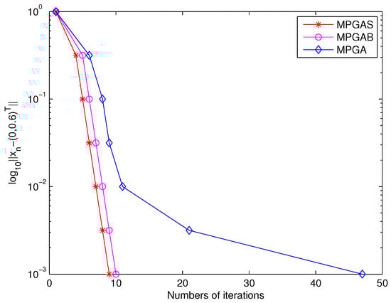
From Table 1 and Figure 1 above, we see that the superiorized version and the bounded perturbation algorithm of (21) arrived at the minimum and the unique minimum point by nine iterations while the original algorithm (21) took 47 iterations to attain the same minimum with the zero initial value. Similar results were also obtained with the initial value $x_0$ from uniform distribution.

We now discuss a general case of problem (47) by the above-mentioned algorithms.

Example 2.

Let the system matrix $A\in {\mathbb{R}}^{50\times 200}$ be stimulated by standard Gaussian distribution, ${\mu }_k=1,k=1,2,\cdots ,200$. Let the vector $d\in {\mathbb{R}}^{50}$ be generated from a uniform distribution in the interval [−2,2]. Solve the optimal problem (47) with the above-mentioned algorithms.

We take the parameters in the algorithms as follows:

1. 

Algorithm parameters:

The contraction $h\left(x\right)=x/3$. The diagonal scaling matrix

$$D\left(x_n\right)=diag\{d_{ii}\left(x_n\right)\}=diag\{1-\frac{1}{n^2}\}.$$

(55)

$t_n=\frac{1}{3n}$, ${\gamma }_n=0.01+\frac{1}{2n}$, then ${\lambda }_n=1-t_n-{\gamma }_n$. The step size sequence ${\alpha }_n=\frac{n}{L(n+1)}$.

2. 

Algorithm parameters for the superiorized version:

The summable nonnegative real sequence $\left\{{\beta }_n\right\}$: ${\beta }_n=c^n$ for some $c\in (0,1)$ and $I=10$. We set ϕ as the objective function in problem (47).

The iteration numbers $“Iter”$, the computing time in seconds (“$CPU\left(s\right)$”), the error’s values (“$Err$”) are reported in Table 2 with a random initial guess $x_0=2\ast rand(200,1)$ when the stopping criterion

$$Err:=\Vert x_{n+1}-x_n{\Vert }_2<\epsilon$$

(56)

is reached, where ε is a given small positive constant.

Table 2. Results for Example 2 with $x_0=2\ast rand(200,1)$.

Methods	$\mathit{Err}<{\mathbf{10}}^{-\mathbf{4}}$			$\mathit{Err}<{\mathbf{10}}^{-\mathbf{6}}$
	Iter	$\mathit{CPU}\left(\mathit{s}\right)$	$\mathit{Obj}$	Iter	$\mathit{CPU}\left(\mathit{s}\right)$	$\mathit{Obj}$
MPGAS	367	4.265625	27.127	1652	3.343750	22.790
MPGAB	1154	5.812500	28.563	2354	7.593750	22.793
MPGA	2084	9.781250	32.386	2354	8.046875	22.793

We find from Table 2 that there is no increase in the execution time of the computer by running the superiorized version, MPGAS, of original algorithm (21). In contrast, compared to the algorithms MPGAB and MPGA, MPGAS even reduces the operation time to get a smaller objective function value under the same stop criterions and initial value $x_0$.

5. Conclusions

In this paper, we have proposed a proximal scaled gradient algorithm with multi-parameters and studied the strong convergence of it in a real Hilbert space for solving a composite optimization problem. We have investigated the bounded perturbation resilience and the superiorized version of it as well. The validity of the proposed algorithm and the comparison of the original iteration, the bounded perturbation form and the superiorized version of it were illustrated by numerical examples. The results and numerical examples in this paper are a new attempt or application of a newly developed superiorization method. It shows that this method works well to some degree for the proposed algorithm.

References

- Censor, Y.; Davidi, R.; Herman, G.T. Perturbation resilience and superiorization of iterative algorithms. Inverse Probl. 2010, 26, 65008. [Google Scholar] [CrossRef] [PubMed]
- Davidi, R.; Schulte, R.W.; Censor, Y.; Xing, L. Fast superiorization using a dual perturbation scheme for proton computed tomography. Trans. Am. Nucl. Soc. 2012, 106, 73–76. [Google Scholar]
- Davidi, R.; Herman, G.T.; Censor, Y. Perturbation-resilient block-iterative projection methods with application to image reconstruction from projections. Int. Trans. Oper. Res. 2009, 16, 505–524. [Google Scholar] [CrossRef] [PubMed]
- Nikazad, T.; Davidi, R.; Herman, G.T. Accelerated perturbation-resilient block-iterative projection methods with application to image reconstruction. Inverse Probl. 2012, 28, 035005. [Google Scholar] [CrossRef] [PubMed]
- Censor, Y.; Chen, W.; Combettes, P.L.; Davidi, R.; Herman, G.T. On the effectiveness of projection methods for convex feasibility problems with linear inequality constraints. Comput. Optim. Appl. 2012, 51, 1065–1088. [Google Scholar] [CrossRef]
- Censor, Y.; Zaslavski, A.J. Strict Fejér monotonicity by superiorization of feasibility-seeking projection methods. J. Optim. Theory Appl. 2015, 165, 172–187. [Google Scholar] [CrossRef]
- Davidi, R.; Censor, Y.; Schulte, R.W.; Geneser, S.; Xing, L. Feasibility-seeking and superiorization algorithm applied to inverse treatment plannning in rediation therapy. Contemp. Math. 2015, 636, 83–92. [Google Scholar]
- Censor, Y.; Zaslavaski, A.J. Convergence and perturbation resilience of dynamic string averageing projection methods. Comput. Optim. Appl. 2013, 54, 65–76. [Google Scholar] [CrossRef]
- Censor, Y.; Davidi, R.; Herman, G.T.; Schulte, R.W.; Tetruashvili, L. Projected subgradient minimization versus superiorization. J. Optim. Theory Appl. 2014, 160, 730–747. [Google Scholar] [CrossRef]
- Dong, Q.L.; Lu, Y.Y.; Yang, J. The extragradient algorithm with inertial effects for solving the variational inequality. Optimization 2016, 65, 2217–2226. [Google Scholar] [CrossRef]
- Garduño, E.; Herman, G. Superiorization of the ML-EM algorithm. IEEE Trans. Nucl. Sci. 2014, 61, 162–172. [Google Scholar]
- He, H.; Xu, H.K. Perturbation resilience and superiorization methodology of averaged mappings. Inverse Probl. 2017, 33, 040301. [Google Scholar] [CrossRef]
- Jin, W.; Censor, Y.; Jiang, M. Bounded perturbation resilience of projected scaled gradient methods. J. Comput. Optim. Appl. 2016, 63, 365–392. [Google Scholar] [CrossRef]
- Schrapp, M.J.; Herman, G.T. Data fusion in X-ray computed tomography using a superiorization approach. Rev. Sci. Instrum. 2014, 85, 055302. [Google Scholar] [CrossRef] [PubMed]
- Guo, Y.N.; Cui, W. Strong convergence and bounded perturbation resilience of a modified proximal gradient algorithm. J. Inequal. Appl. 2018, 2018, 103. [Google Scholar] [CrossRef] [PubMed]
- Zhu, J.H.; Penfold, S. Total variation superiorization in dualenergy CT reconstruction for proton therapy treatment planning. Inverse Probl. 2017, 33, 044013. [Google Scholar] [CrossRef]
- Zibetti, M.V.W.; Lin, C.A.; Herman, G.T. Total variation superiorized conjugate gradient method for image reconstruction. Inverse Probl. 2018, 34, 034001. [Google Scholar] [CrossRef]
- Bauschke, H.H.; Combettes, P.L. Convex Analysis and Monotone Operator Theory in Hilbert Space; Dilcher, K., Taylor, K., Eds.; Springer: New York, NY, USA, 2011. [Google Scholar]
- Xu, H.K. Properties and Iterative Methods for the Lasso and Its Variants. Chin. Ann. Math. 2014, 35, 501–518. [Google Scholar] [CrossRef]
- Strand, O.N. Theory and methods related to the singular-function expansion and Landweber iteration for integral equations of the first kind. SIAM J. Numer. Anal. 1974, 11, 798–825. [Google Scholar] [CrossRef]
- Piana, M.; Bertero, M. Projected Landweber method and preconditioning. Inverse Probl. 1997, 13, 441–463. [Google Scholar] [CrossRef]
- Neto, E.S.; Helou, D.; Álvaro, R. Convergence results for scaled gradient algorithms in positron emission tomography. Inverse Probl. 2005, 21, 1905–1914. [Google Scholar] [CrossRef]
- Guo, Y.N.; Cui, W.; Guo, Y.S. Perturbation resilience of proximal gradient algorithm for composite objectives. J. Nonlinear Sci. Appl. 2017, 10, 5566–5575. [Google Scholar] [CrossRef][Green Version]
- Xu, H.K. Iterative methods for the split feasibility problem in infinite-dimensional Hilbert space. Inverse Probl. 2010, 26, 105018. [Google Scholar] [CrossRef]
- Moreau, J.J. Proximité et dualité dans un espace hilbertien. Bull. Soc. Math. Fr. 1965, 93, 273–299. [Google Scholar] [CrossRef]
- Marino, G.; Xu, H.K. Convergence of generalized proximal point algorithm. Commun. Pure Appl. Anal. 2004, 3, 791–808. [Google Scholar]
- Xu, H.K. Iterative algorithms for nonlinear operators. J. Lond. Math. Soc. 2002, 66, 240–256. [Google Scholar] [CrossRef]
- Xu, H.K. Error sensitivity for strongly convergent modifications of the proximal point algorithm. J. Optim. Theory Appl. 2015, 168, 901–916. [Google Scholar]
© 2019 by the authors. Licensee MDPI, Basel, Switzerland. This article is an open access article distributed under the terms and conditions of the Creative Commons Attribution (CC BY) license (http://creativecommons.org/licenses/by/4.0/).