The Second-Order Shape Derivative of Kohn–Vogelius-Type Cost Functional Using the Boundary Differentiation Approach

Abstract

A shape optimization method is used to study the exterior Bernoulli free boundary problem. We minimize the Kohn–Vogelius-type cost functional over a class of admissible domains subject to two boundary value problems. The first-order shape derivative of the cost functional is recalled and its second-order shape derivative for general domains is computed via the boundary differentiation scheme. Additionally, the second-order shape derivative of J at the solution of the Bernoulli problem is computed using Tiihonen’s approach.

1. Introduction

Nowadays many researchers are interested in a class of boundary value problems called free boundary problems. These are mostly partial differential equations to be solved for both unknown state function(s) and an unknown domain. It is called “free boundary” because the boundary or part of the boundary of the domain is not known in advance, and usually this terminology is used to indicate that the boundary is stationary and a steady state problem exists. Sometimes this term is used to refer to the so-called moving boundaries. However, moving boundary problems are usually associated to problems that vary with time.

A typical example of the free boundary problem is the melting of a solid that occupies a domain Ω inside a container U. Assuming that the container has a liquid occupying $\Gamma =U\backslash \Omega$, with an initial temperature distribution $T(0,x)$, and suppose we can control $\partial U$ at any time. Then, knowing these properties, one can reconstruct the solid-liquid configuration ${\Omega }_t$ and ${\Gamma }_t$, and the temperature distribution $T(t,x)$ at any time $t>0$. Ideally, the temperature should satisfy some type of diffusion equation in ${\Omega }_t$ and ${\Gamma }_t$, and on the interface some “balance” conditions that would describe the dynamics of the melting process must be satisfied. These “balance conditions” will then define the boundary separating the solid and the liquid. To construct solutions to this type of problems, one can try to build “classical solutions” in the sense that ${\Omega }_t$ and ${\Gamma }_t$ are smooth, T is smooth up to the boundary $\partial {\Omega }_t$, and the interphase conditions on T are satisfied pointwise. For further discussion, see [2].

Free boundary problems are not confined only to the study of phase transitions, such as that of solidification or melting of a particular material, or to the study of fluid dynamics. They also arise in the study of image development in electrophotography, chemical vapor deposition, and tumor growth [3]. Due to their remarkably wide range of new and challenging applications in real life, they are being extensively studied in other disciplines such as combustion, electrochemical machining, molecular diffusion, steel and glass production, and flame propagation, among others [2,4,5,6,7].

This paper studies a class of two-dimensional free boundary problems of Bernoulli type. This class of problems has applications to electrochemical machining, fluid mechanics, optimal insulation, electrical impedance tomography, among others [2,3,5,6,7,8]. In this paper, we are interested in the exterior Bernoulli problem (BP), which can be described as follows: Given a bounded and connected domain $A\subset {\mathbb{R}}^2$ with a fixed boundary $\Gamma :=\partial A$ and a constant $\lambda <0$, one needs to find a bounded connected domain $B\subset {\mathbb{R}}^2$ with a free boundary Σ and containing the closure of A, and an associated state function $u:\Omega \to \mathbb{R}$, where $\Omega =B\setminus \overline{A}$, such that the following conditions are met:

$$\left\{\begin{array}{cc}\hfill -\Delta u=0& in \Omega ,\\ \hfill u=1& on \Gamma ,\\ \hfill u=0& on \Sigma ,\\ \hfill {\displaystyle \frac{\partial u}{\partial \mathbf{n}}}=\lambda & on \Sigma ,\end{array}\right.$$

(1)

where $\mathbf{n}$ refers to the outward unit normal vector to Σ. Details about the exterior Bernoulli problems can be seen, for instance, in [4,6,9,10,11,12,13,14,15]. The presence of overdetermined conditions on Σ makes the problem difficult to solve. Shape optimization method, however, is an established tool in solving such problems. One way to reformulate the problem is as follows:

$$\underset{\Omega }{min}J(\Omega )\equiv \underset{\Omega }{min}{\displaystyle \frac{1}{2}}{\int }_{\Omega }{\left|\nabla (u_D-u_N)\right|}^2\text{d}x$$

(2)

over all admissible domains Ω, where the state function $u_D$ is the solution to the Dirichlet problem:

$$\left\{\begin{array}{cc}\hfill -\Delta u_D=0& \text{in} \Omega ,\\ \hfill u_D=1& \text{on} \Gamma ,\\ \hfill u_D=0& \text{on} \Sigma ,\end{array}\right.$$

(3)

and the state function $u_N$ is the solution to the Neumann problem:

$$\left\{\begin{array}{cc}\hfill -\Delta u_N=0& \text{in} \Omega ,\\ \hfill u_N=1& \text{on} \Gamma ,\\ \hfill {\displaystyle \frac{\partial u_N}{\partial \mathbf{n}}}=\lambda & \text{on} \Sigma .\end{array}\right.$$

(4)

The functional J is sometimes called Kohn–Vogelius (KV) cost functional because Kohn and Vogelius were among the first to use it in the context of inverse conductivity problems [16]. The idea behind this formulation is that any domain at which the KV functional vanishes is a solution of the Bernoulli problem and vice versa.

Minimizing a shape functional requires, most of the time, some gradient information and Hessian. The first-order shape derivative of KV functional has already been carried out (cf. [17,18]). We have done it in two different ways. One is through variational means similar to the techniques developed in [12,13,19], wherein we use the Hölder continuity of the state variables satisfying the Dirichlet and Neumann problems but we do not introduce any adjoint variables. The other is by using the shape or material derivatives of the states in a rigorous manner (cf. [20]). In [17], the authors used the KV functional for the numerical solution of the Bernoulli problem but restricted to starlike domains, while the authors in [4] considered it in general domains. The second-order shape derivative was also computed in [21] using the approach by Sokolowski and Zolesio [22] and by domain differentiation technique. This is also different from the work of Eppler and Harbrect (cf. [17,23]) where computation is restricted only to starlike shapes. Material derivatives, as well as shape derivatives of the state variables, are highly involved in the approach that we used.

2. Outline of the work

The rest of the paper is outlined as follows:

Section 3 provides a list of tools that are needed in the analysis for the shape derivatives of the Kohn-Vogelius cost functional. Here we describe the reference domain and the perturbed domains that are considered in the work. We introduce the perturbation of identity operator $T_t$ and prove several properties of it. Since we study functions living in different domains, this section also discusses the method of mapping, from which the concepts of material and shape derivatives arise. The domain and boundary transformation formulas, and several formulas in tangential calculus are provided in this section. Also, a discussion on the structure of the second order Eulerian derivative of a general shape functional is presented.

Using the tools presented in Section 3, our main contribution for the second-order shape derivative of J is being discussed in Section 4. The derivation is done on a formal manner. In this section, we recall the domain ${\Omega }_{t,s}$ which is needed in characterizing the second order Eulerian derivative of J. But first we provide results on the shape and material derivatives of $\mathbf{n}$, τ and κ. These, together with the material and shape derivatives of the states, are used in the computation of the second-order shape derivative of J. The approach used in computing is based on a method which make use of boundary differentiation formula that is taken from [24]. Though it is not yet established the advantage of using this method from that of Sokolowski and Zolesio [22], this method has a gain over the domain differentiation approach presented in [21]. First, it does not require the use of Stoke’s theorem and second, most of the tools used are tangential calculus results. We show that the computed shape derivative has a symmetric and nonsymmetric part, and in general it satisfies a structure theorem. Finally, the second-order Eulerian derivative of J at the solution of the Bernoulli problem is discussed using the Tiihonen’s approach [1], wherein the general explicit expression of the second-order shape derivative is not used. We compared this to the result wherein the explicit form is utilized.

3. Preliminaries

3.1. Properties of the Perturbation of Identity Operator

In this work we consider two-dimensional bounded connected domains Ω of class $C^{k,1}$, $k\ge 1$, that are subsets of a hold-all domain U. Moreover, Ω is an annulus having an inner fixed boundary Γ that is disjoint from an external free boundary Σ. The vector fields $\mathbf{V}$ considered in the paper are those belonging to the space Θ defined by

$$\Theta =\left\{\mathbf{V}\in C^{1,1}(\overline{U},{\mathbb{R}}^2){:\mathbf{V}|}_{\Gamma \cup \partial U}=0\right\}.$$

(5)

The domain Ω is deformed using the perturbation of identity operator

$$T_t:\overline{U}\to {\mathbb{R}}^2,T_t\left(x\right)=x+t\mathbf{V}\left(x\right),x\in \overline{U},$$

(6)

where $\mathbf{V}\in \Theta .$ For $t=0$, we have the reference domain $\Omega :={\Omega }_0$, with a fixed boundary $\Gamma :={\Gamma }_0$ and a free boundary $\Sigma :={\Sigma }_0$. For a given $t>0$ we denote the deformed domain to be ${\Omega }_t$, with a fixed boundary ${\Gamma }_t$ and a free boundary ${\Sigma }_t$.

We use the following notations in our work:

$$\begin{array}{cccccc}\hfill I_t\left(x\right)& =& detD{T}_t\left(x\right),x\in \overline{U},\hfill & \hfill M_t\left(x\right)& =& {\left(D{T}_t\left(x\right)\right)}^{-T},x\in \overline{U},\hfill \\ \hfill A_t\left(x\right)& =& I_t{M}_t^T{M}_t\left(x\right),x\in \overline{U},\hfill & \hfill w_t\left(x\right)& =& I_t\left(x\right)\left|{\left(D{T}_t\left(x\right)\right)}^{-T}\mathbf{n}\left(x\right)\right|,x\in \Sigma .\hfill \end{array}$$

(7)

The determinant $I_t$ has the following property, which is used to prove the next theorem.

Lemma 1 ([12,19]). Consider the operator $T_t$ defined by Equation (6), where $\mathbf{V}\in \Theta$, which is described by Equation (5). Then

• $I_t=1+tdiv\mathbf{V}+t^{2}detD\mathbf{V}$, and
• there exists $t_V,{\alpha }_1,{\alpha }_2>0$ such that $0<{\alpha }_1\le I_t\left(x\right)\le {\alpha }_2$, for $\left|t\right|\le t_V,x\in U$.

Theorem 1 ([18]). Let Ω and U be nonempty bounded open connected subsets of ${\mathbb{R}}^2$ with Lipschitz continuous boundaries, such that $\overline{\Omega }\subseteq U$, and $\partial \Omega$ is the union of two disjoint boundaries Γ and Σ. Let $T_t$ be defined as in Equation (6) where $\mathbf{V}$ belongs to Θ, defined by Equation (5). Then for sufficiently small t,

• $T_t:\overline{U}\to \overline{U}$ is a homeomorphism,
• $T_t:U\to U$ is a $C^{1,1}$ diffeomorphism, and in particular, $T_t:\Omega \to {\Omega }_t$ is a $C^{1,1}$ diffeomorphism,
• ${\Gamma }_t=T_t(\Gamma )=\Gamma$, ${\Sigma }_t=T_t(\Sigma )$ and $\partial {\Omega }_t=\Gamma \cup {\Sigma }_t$.

Here are some properties of $T_t$ that are relevant to our work.

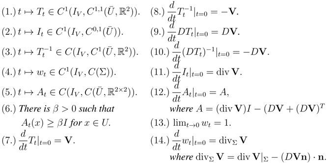
Lemma 2 ([12,19]). Consider the transformation $T_t$, where the fixed vector field $\mathbf{V}$ belongs to Θ, defined in Equation (5). Then there exists $t_V>0$ such that $T_t$ and the functions in Equation (7) restricted to the interval $I_V=(-t_V,t_V)$ have the following regularity and properties:

We perturb the reference domain twice to discuss the second-order shape derivative of the functional. We define the transformations $T_t^{\mathbf{V}}:\overline{U}\to {\mathbb{R}}^2$ and $T_s^{\mathbf{W}}:\overline{U}\to {\mathbb{R}}^2$ by $T_t^{\mathbf{V}}\left(x\right)=(I+t\mathbf{V})\left(x\right),$ and $T_s^{\mathbf{W}}\left(y\right)=(I+s\mathbf{W})\left(y\right),x,y\in \overline{U}$ where $\mathbf{V},\mathbf{W}\in \Theta$, but for simplicity, we denote $T_t$ the transformation $T_t^{\mathbf{V}}$ in the direction $\mathbf{V}$ and $T_s:=T_s^{\mathbf{W}}$. Using Theorem 1, the mapping $T_{t,s}:=T_t\circ T_s:\Omega \to {\Omega }_{t,s}$, defined by

$$T_{t,s}\left(x\right):=T_t\left(T_s\left(x\right)\right)=x+s\mathbf{W}\left(x\right)+t\mathbf{V}(x+s\mathbf{W}\left(x\right)),x\in \Omega$$

(8)

is a $C^{1,1}$ diffeomorphism. We now define the perturbed domain ${\Omega }_{t,s}$ as:

$$\begin{array}{c}\hfill {\Omega }_{t,s}:=T_t\left(T_s(\Omega )\right):=\{T_{t,s}\left(x\right):x\in \Omega \}.\end{array}$$

(9)

Hence, for sufficiently small t and s, ${\Omega }_t,{\Omega }_{t,s}\in C^{1,1}$, and they are contained in U. The new free boundary after two deformations becomes

$${\Sigma }_{t,s}:=T_t\left(T_s(\Sigma )\right):=(T_t\circ T_s(\Sigma )):=T_t\left({\Sigma }_s\right),$$

and clearly ${\Gamma }_{t,s}=\Gamma$. We emphasize that ${\Omega }_{t,s}$ should not be thought of as the domain obtained through deforming the initial domain Ω in the direction of the resultant vector field $t\mathbf{V}+s\mathbf{W}$. The latter perturbed domain is defined by ${\Omega }_{t+s}=\{x+(t\mathbf{V}+s\mathbf{W})\left(x\right):x\in \Omega \}$, while elements of ${\Omega }_{t,s}$ are given by Equation (8). In general ${\Omega }_{t,s}\ne {\Omega }_{t+s}$, as shown in Figure 1. In particular, if $\mathbf{V}=\mathbf{W}$, we get for $x\in \Omega$,

$$T_{t+s}\left(x\right)=x+(t+s)\mathbf{V}\left(x\right),\text{while}{T}_{t,s}\left(x\right)=x+t\mathbf{V}\left(x\right)+s\mathbf{V}(x+t\mathbf{V}\left(x\right)).$$

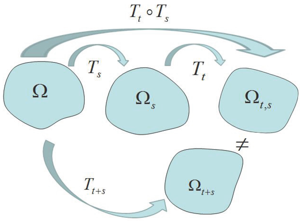
Figure 1. The difference between domains ${\Omega }_{t,s}$ and ${\Omega }_{t+s}$.

3.2. Concepts in the Method of Mapping

Definition 1 ([1,25]). Let u be defined in $[0,t_V]\times U$. An element $\dot{u}\in H^k(\Omega )$, called the material derivative of u, is defined as

$$\dot{u}\left(x\right):=\dot{u}(0,x):=\underset{t\to 0^{+}}{lim}{\displaystyle \frac{u(t,T_t\left(x\right))-u(0,x)}{t}}={\displaystyle \frac{d}{dt}}u(t,x+t\mathbf{V}\left(x\right)){|}_{t=0},$$

if the limit exists (in $H^k(\Omega )$).

Definition 2. Let u be defined in $[0,t_V]\times U$. An element $u^{\prime }\in H^k(\Omega )$ is called the shape derivative of u at Ω in the direction $\mathbf{V}$, if the following limit exists in $H^k(\Omega )$:

$$u^{\prime }\left(x\right):=u^{\prime }(0,x):=\underset{t\to 0^{+}}{lim}{\displaystyle \frac{u(t,x)-u(0,x)}{t}}:=\dot{u}\left(x\right)-(\nabla u·\mathbf{V})\left(x\right).$$

(10)

Remark 1. As noted in [21], the material and shape derivative of vector-valued functions can also be defined. Similar to Definition 1, if $\mathbf{u}:[0,t_V]\times U\to {\mathbb{R}}^n$ belongs to $H^k(\Omega ;{\mathbb{R}}^n)$ then its material derivative in the direction $\mathbf{V}$ can be written as

$$\dot{\mathbf{u}}\left(x\right):=\dot{\mathbf{u}}(\Omega ;\mathbf{V})=\underset{t\to 0^{+}}{lim}{\displaystyle \frac{\mathbf{u}(t,T_t\left(x\right))-\mathbf{u}(0,x)}{t}}={\displaystyle \frac{d}{dt}}\mathbf{u}(t,x+t\mathbf{V}\left(x\right)){|}_{t=0},$$

(11)

whenever the limit exists (in $H^k(\Omega ,{\mathbb{R}}^n)$). If its shape derivative also exists then the following relation holds:

$${\mathbf{u}}^{\prime }\left(x\right)=\dot{\mathbf{u}}\left(x\right)-\left(D\mathbf{u}\mathbf{V}\right)\left(x\right).$$

(12)

If $\mathbf{u}=(u_1,u_2)$ then its norm is given by ${\left|\mathbf{u}\right|}_{H^k(\Omega ,{\mathbb{R}}^2)}=|u_1{|}_{H^k(\Omega )}+{\left|u_2\right|}_{H^k(\Omega )}$ for $k\ge 0.$.

Lemma 3 ([19,22], Domain and Boundary Transformations).

• Let ${\phi }_t\in L^1\left({\Omega }_t\right)$. Then ${\phi }_t\circ T_t\in L^1(\Omega )$ and

  $${\int }_{{\Omega }_t}{\phi }_t\text{d}{x}_t={\int }_{\Omega }{\phi }_t\circ T_t{I}_t\text{d}x.$$
• Let ${\phi }_t\in L^1\left(\partial {\Omega }_t\right)$. Then ${\phi }_t\circ T_t\in L^1(\partial \Omega )$ and

  $${\int }_{\partial {\Omega }_t}{\phi }_t\text{d}{s}_t={\int }_{\partial \Omega }{\phi }_t\circ T_t{w}_t\text{d}s,$$

  where $I_t$ and $w_t$ are defined in Equation (7).

Definition 3 ([22,24,26,27]).

• The tangential gradient of $f\in C^1(\Gamma )$ is given by

  $${\nabla }_{\Gamma }{f:=\nabla F|}_{\Gamma }-{\displaystyle \frac{\partial F}{\partial \mathbf{n}}}\mathbf{n}\in C(\Gamma ,{\mathbb{R}}^n).$$

  (13)
• The tangential Jacobian matrix of a vector function $\mathbf{v}\in C^1(\Gamma ,{\mathbb{R}}^n)$ is given by

  $$D_{\Gamma }{\mathbf{v}=D\mathbf{V}|}_{\Gamma }-\left(D\mathbf{V}\mathbf{n}\right){\mathbf{n}}^T\in C(\Gamma ,{\mathbb{R}}^{n\times n}).$$

  (14)
• The tangential divergence of a vector function $\mathbf{v}\in C^1(\Gamma ,{\mathbb{R}}^n)$ on Γ is given by

  $${div}_{\Gamma }{\mathbf{v}=div\mathbf{V}|}_{\Gamma }-D\mathbf{V}\mathbf{n}·\mathbf{n}\in C(\Gamma ),$$

  (15)

  where $\mathbf{F}$ and $\mathbf{V}$ are any corresponding $C^1$ extensions of f and $\mathbf{v}$ into a neighborhood of Γ.

Lemma 4 ([22]). Consider a $C^2$ domain Ω with boundary $\Gamma :=\partial \Omega$. Then for $u\in H^1(\Gamma )$ and $\mathbf{V}\in C^1(\Gamma ,{\mathbb{R}}^n)$ the following identities hold:

$$\begin{array}{ccc}& & \left(1\right){div}_{\Gamma }\left(u\mathbf{V}\right)={\nabla }_{\Gamma }u·\mathbf{V}+u{div}_{\Gamma }\mathbf{V},\hfill \end{array}$$

(16)

$$\begin{array}{ccc}& & \left(2\right){\int }_{\Gamma }{div}_{\Gamma }\mathbf{V}ds={\int }_{\Gamma }\kappa \mathbf{V}·\mathbf{n}ds,\hfill \end{array}$$

(17)

$$\begin{array}{ccc}& & \left(3\right){\int }_{\Gamma }(u{div}_{\Gamma }\mathbf{V}+{\nabla }_{\Gamma }u·\mathbf{V})ds={\int }_{\Gamma }\kappa u\mathbf{V}·\mathbf{n}ds,\hfill \end{array}$$

(18)

$$\begin{array}{ccc}& & \left(4\right){\int }_{\Gamma }{\nabla }_{\Gamma }u·\mathbf{V}ds=-{\int }_{\Gamma }u{div}_{\Gamma }\mathbf{V}ds,where\mathbf{V}·\mathbf{n}=0.\hfill \end{array}$$

(19)

Remark 2. In Lemma 4, the first identity is called the tangential divergence formula, the second is commonly known as the tangential Stoke’s formula, and the third is referred to as the tangential Green’s formula. These formulas are also valid for $C^{1,1}$ domains.

The following is also another version of the tangential Green’s formula.

Lemma 5 ([12,28]). Let U be a bounded domain of class $C^{1,1}$ and $\Omega \subset U$ with boundary Γ. Also, consider $\mathbf{V}\in C^{1,1}(\overline{U},{\mathbb{R}}^n)$ and $u\in W^{2,1}\left(U\right)$. Then

$${\int }_{\Gamma }(u{div}_{\Gamma }\mathbf{V}+\nabla u·\mathbf{V})\text{d}s={\int }_{\Gamma }\left({\displaystyle \frac{\partial u}{\partial \mathbf{n}}}+\kappa u\right)\mathbf{V}·\mathbf{n}\text{d}s.$$

(20)

Theorem 2 ([22], Boundary Differentiation Formula). Let u be defined in a neighborhood of a boundary $\partial \Omega$ of a $C^{1,1}$ domain Ω. If $u\in C(I_V,W^{2,1}\left(U\right))$ and $\dot{u}(0,·)\in W^{1,1}\left(U\right)$, then

$${\displaystyle \frac{d}{dt}}{\int }_{{\Sigma }_t}u(t,s)\text{d}s{|}_{t=0}={\int }_{\Sigma }{u}^{\prime }(0,s)\text{d}s+{\int }_{\Sigma }({\displaystyle \frac{\partial u}{\partial \mathbf{n}}}+u(0,s)\kappa )\mathbf{V}·\mathbf{n}\text{d}s,$$

(21)

where κ is the mean curvature of the free boundary Σ.

Definition 4.

• The first-order Eulerian derivative of a shape functional $J:\Omega \to \mathbb{R}$ at the domain Ω in the direction of the deformation field $\mathbf{V}$ is given by

  $$dJ(\Omega ;\mathbf{V}):=\underset{t\to 0^{+}}{lim}{\displaystyle \frac{J\left({\Omega }_t\right)-J(\Omega )}{t}},$$

  (22)

  if the limit exists.
• The second-order Eulerian derivative of J at the domain Ω in the direction of the deformation fields $\mathbf{V}$ and $\mathbf{W}$ is given by

  $$d^{2}J(\Omega ;\mathbf{V},\mathbf{W})=\underset{s\to 0^{+}}{lim}{\displaystyle \frac{dJ({\Omega }_s\left(\mathbf{W}\right),\mathbf{V})-dJ(\Omega ;\mathbf{V})}{s}}=:{\displaystyle \frac{\partial }{\partial s}}\left\{{\displaystyle \frac{\partial }{\partial t}}J\left({\Omega }_{t,s}\right){|}_{t=0}\right\}{|}_{s=0},$$

  (23)

  if the limit exists. Here, ${\Omega }_{t,s}$ is defined by Equation (9).

Remark 3. J is said to be shape differentiable at Ω if $dJ(\Omega ;\mathbf{V})$ exists for all $\mathbf{V}$ and is linear and continuous with respect to $\mathbf{V}$. It is twice shape differentiable if for all $\mathbf{V}$ and $\mathbf{W}$, $d^{2}J(\Omega ;\mathbf{V},\mathbf{W})$ exists and if $d^{2}J(\Omega ;\mathbf{V},\mathbf{W})$ is bilinear and continuous with respect to $\mathbf{V}$ and $\mathbf{W}$.

3.3 Anatomy of the Second-Order Shape Derivative

Using the perturbation of identity, one can decompose the expression $d^{2}J(\Omega ;\mathbf{V},\mathbf{W})$ into symmetric and non-symmetric terms (cf. [24], p. 384). The non-symmetric part is obtained from the first-order shape derivative applied to the deformation field $D\mathbf{V}\mathbf{W}$. This is investigated by Novruzi and Pierre [29] by using the perturbation of identity technique presented in [28,30]. The structure of the shape derivative of functional J uses the fact that any regular small perturbation ${\Omega }_{\theta }:=(I+\theta )(\Omega )$ of a smooth domain Ω (where θ is a sufficiently smooth mapping from ${\mathbb{R}}^n$ to ${\mathbb{R}}^n$) can be uniquely represented up to a “shift" on Γ by a normal deformation to Γ. For completeness, we give some details of it, which is taken from [29].

For any $l\in \mathbb{N},1\le l\le k$, we denote

$$G^{k-l}(\Gamma ,\Gamma )=\left\{g\in C^{k-l}(\Gamma ,{\mathbb{R}}^n):g(\Gamma )\subset \Gamma \right\}.$$

(24)

Lemma 6. Let Ω denote a bounded domain with $C^k$ boundary Γ. Then for any $1\le l\le k,$

(i)

there exists an open neighborhood $N_k$ of 0 in

$${\Theta }_k=\left\{\mathbf{V}\in C^k({\mathbb{R}}^n,{\mathbb{R}}^n):derivatives of \mathbf{V} up to order k are bounded.\right\},$$

(25)

and $C^l$ functions $\Psi :N_k\to C^{k-l}(\Gamma )$ and $\Phi :N_k\to G^{k-l}(\Gamma ,\Gamma )$ such that for any $\theta \in N_k$,

$$(I+\theta )\circ \Phi \left(\theta \right)=I+\Psi \left(\theta \right)\mathbf{n}on \Gamma .$$

(26)

(ii)

Moreover, the values of the first- and second-order (Fréchet) derivatives of Ψ at $\theta =0$ in the directions $\mathbf{V},\mathbf{W}\in {\Theta }_k$ are given by

(a)

$D_{\theta }\Psi \left(0\right)\left(\mathbf{V}\right):={\Psi }^{\prime }\left(0\right)\left(\mathbf{V}\right)=\mathbf{v}·\mathbf{n}forl\ge 1$, and

(b)

$D_{\theta }^2\Psi \left(0\right)(\mathbf{V},\mathbf{W}):={\Psi }^{\prime \prime }\left(0\right)(\mathbf{V},\mathbf{W})=-v_{\Gamma }·D_{\Gamma }\mathbf{n}{w}_{\Gamma }-\mathbf{n}·D_{\Gamma }\mathbf{v}{w}_{\Gamma }-\mathbf{n}·D_{\Gamma }\mathbf{w}{v}_{\Gamma }$ for $l\ge 2$, where ${\mathbf{v}=\mathbf{V}|}_{\Gamma }$ and ${\mathbf{w}=\mathbf{W}|}_{\Gamma }$.

The implicit function theorem is used to prove the lemma. Consequently, this lemma is used to prove the next result, where $O_k$ refers to the set of bounded $C^k$ domains.

Theorem 3. [29, p.368] Consider the shape functional $J:O_k\to \mathbb{R}$ and the functional $\mathbf{J}:{\overline{\Theta }}_k\to \mathbb{R}$ where

$${\overline{\Theta }}_k:=\left\{\theta \in {\Theta }_k:{\left|\theta \right|}_{C^k}<1\right\},and\mathbf{J}\left(\theta \right)=J\left({\Omega }_{\theta }\right).$$

(27)

For $k\ge 1$, the following statements hold.

(i)

If $\Omega \in O_{k+1}$ and $\mathbf{J}$ is differentiable at 0 in ${\Theta }_k$, then there is a continuous linear map $l_1:C^k(\Gamma )\to \mathbb{R}$ such that for any $\mathbf{V}\in {\Theta }_k$,

$$D_{\theta }\mathbf{J}\left(0\right)\left(\mathbf{V}\right):={\mathbf{J}}^{\prime }\left(0\right)\left(\mathbf{V}\right)=l_1(\mathbf{v}·\mathbf{n}).$$

(28)

(ii)

If $\Omega \in O_{k+1}$ and $\mathbf{J}$ is twice differentiable at 0 in ${\Theta }_k$ then there exists a continuous bilinear symmetric map $l_2:C^k(\Gamma )\times C^k(\Gamma )\to \mathbb{R}$ such that for any $\mathbf{V},\mathbf{W}\in {\Theta }_{k+1}$ we have

$$\begin{array}{c}{D}_{\theta }^2\mathbf{J}\left(0\right)(\mathbf{V},\mathbf{W}):={\mathbf{J}}^{\prime \prime }\left(0\right)(\mathbf{V},\mathbf{W})\hfill \\ \mathrm{(29)}& =l_2(\mathbf{v}·\mathbf{n},\mathbf{w}·\mathbf{n})-l_1(v_{\Gamma }·D_{\Gamma }\mathbf{n}{w}_{\Gamma }+\mathbf{n}·D_{\Gamma }\mathbf{v}{w}_{\Gamma }+\mathbf{n}·D_{\Gamma }\mathbf{w}{v}_{\Gamma }).\hfill \end{array}$$

Here, $\mathbf{v}$ and $\mathbf{w}$ are restrictions of $\mathbf{V}$ and $\mathbf{W}$ on Γ, respectively.

Upon computing the second-order shape derivative of J in the directions $\mathbf{V}$ and $\mathbf{W}$, one can show (cf. [29]) that $d^{2}J(\Omega ;\mathbf{V},\mathbf{W})$ can be written as

$$d^{2}J(\Omega ;\mathbf{V},\mathbf{W})={\mathbf{J}}^{\prime \prime }\left(0\right)(\mathbf{V},\mathbf{W})+{\mathbf{J}}^{\prime }\left(0\right)\left(D\mathbf{V}\mathbf{W}\right),$$

(30)

where $J^{\prime \prime }$ and $J^{\prime }$ are the shape derivatives defined in Equations (29) and (28), respectively.

4. Main Results

We now present the shape derivative method that we used in obtaining the second-order shape derivative of the Kohn–Vogelius functional J. This time, we assume that the domains, deformation vectors, the state variables and the rest of the functions involved are regular enough. We use material and shape derivatives of the states $u_D$ and $u_N$, as well as the material and shape derivatives of $\mathbf{n}$, τ and κ. Additional tools on tangential calculus are used in the simplification. Steklov–Poincaré operators are also introduced in the discussion.

Throughout the discussion, we let ${\mathbf{v}=\mathbf{V}|}_{\Sigma }$ and $\mathbf{v}={\mathbf{v}}_{\Sigma }+v_n\mathbf{n}$, where the vector ${\mathbf{v}}_{\Sigma }$ is the tangential component of $\mathbf{v}$ and the scalar $v_n:=\mathbf{v}·\mathbf{n}$ is referred to as its normal component. We remark here that for a given scalar function f and vector function $\mathbf{V}$ defined on the free boundary Σ, the gradient $\nabla f$, the Jacobian $D\mathbf{V}$ and divergence $div\mathbf{V}$ refer actually to the gradient, Jacobian, and divergence of their respective extensions defined on a neighborhood of Σ. For $\mathbf{V}=\mathbf{n}$, we consider a unitary extension $\mathbf{N}$, which gives ${\mathbf{n}}^{T}D\mathbf{N}=0$ and ${D\mathbf{N}|}_{\Sigma }:=D\mathbf{n}=D_{\Sigma }\mathbf{n}$.

Our main result requires the following theorems, which are stated and proven in [21,22,24].

Theorem 4. The material derivative ${\dot{\mathbf{n}}}_W$ and shape derivative ${\mathbf{n}}_W^{\prime }$ of the outward unit normal vector $\mathbf{n}$ at the boundary Σ in the direction of the deformation field $\mathbf{W}$ are given by

$$\begin{array}{ccc}& \left(i\right)& {\dot{\mathbf{n}}}_W=(D\mathbf{W}\mathbf{n}·\mathbf{n})\mathbf{n}-{\left(D\mathbf{W}\right)}^T\mathbf{n},\hfill \end{array}$$

(31)

$$\begin{array}{ccc}& \left(ii\right)& {\mathbf{n}}_W^{\prime }=(D\mathbf{W}\mathbf{n}·\mathbf{n})\mathbf{n}-{\left(D\mathbf{W}\right)}^T\mathbf{n}-\left(D\mathbf{n}\right)\mathbf{W}.\hfill \end{array}$$

(32)

Theorem 5. The material derivative ${\dot{\mathbf{n}}}_W$ and shape derivative ${\mathbf{n}}_W^{\prime }$ of the mean curvature κ of the free boundary Σ in the direction of the deformation field $\mathbf{W}$ are given by

$$\begin{array}{ccc}& \left(i\right)& {\dot{\kappa }}_W=Tr\left[D\left((D\mathbf{W}\mathbf{n}·\mathbf{n})\mathbf{n}-{\left(D\mathbf{W}\right)}^T\mathbf{n}\right)-D\mathbf{n}D\mathbf{W}\right],\hfill \end{array}$$

(33)

$$\begin{array}{ccc}& \left(ii\right)& {\kappa }_W^{\prime }=Tr\left[D\left((D\mathbf{W}\mathbf{n}·\mathbf{n})\mathbf{n}-{\left(D\mathbf{W}\right)}^T\mathbf{n}\right)-D\mathbf{n}D\mathbf{W}\right]-\nabla \kappa ·\mathbf{W}.\hfill \end{array}$$

(34)

Theorem 6. The material derivative ${\dot{\tau }}_W$ and shape derivative ${\tau }_W^{\prime }$ of the unit tangent vector τ on the boundary Σ in the direction of the deformation field $\mathbf{W}$ are given by

$$\begin{array}{ccc}& \left(i\right)& {\dot{\tau }}_W=[{\left(D\mathbf{W}\right)}^T\mathbf{n}·\tau ]\mathbf{n},\hfill \end{array}$$

(35)

$$\begin{array}{ccc}& \left(ii\right)& {\tau }_W^{\prime }=[{\left(D\mathbf{W}\right)}^T\mathbf{n}·\tau ]\mathbf{n}-\left(D\tau \right)\mathbf{W}.\hfill \end{array}$$

(36)

In addition to the tools given in the preliminary section, we present some identities in tangential calculus that are significant to our work on the second-order shape derivative of J.

First we observe that

$${\nabla }_{\Sigma }{v}_n·\mathbf{n}=0.$$

(37)

Second, we observe that

$$\kappa v_n={div}_{\Sigma }\left(v_n\mathbf{n}\right).$$

(38)

This follows from ${div}_{\Sigma }\left(v_n\mathbf{n}\right)={\nabla }_{\Sigma }{v}_n·\mathbf{n}+v_n{div}_{\Sigma }\mathbf{n}$, Equation (37), and the definition of curvature. Here are the other results that are useful to our work (cf. [24]).

Lemma 7. Consider two deformation fields $\mathbf{V}$ and $\mathbf{W}$ that are sufficiently smooth on a neighborhood of Σ, and let ${\mathbf{v}=\mathbf{V}|}_{\Sigma }$ and ${\mathbf{w}=\mathbf{W}|}_{\Sigma }$. Let $\mathbf{v}={\mathbf{v}}_{\Sigma }+v_n$ and $\mathbf{w}={\mathbf{w}}_{\Sigma }+w_n\mathbf{n}$. Then the following identities hold:

$$\begin{array}{ccc}& \left(i\right)& {\left(D_{\Sigma }\mathbf{v}\right)}^T\mathbf{n}={\nabla }_{\Sigma }{v}_n-D\mathbf{n}{\mathbf{v}}_{\Sigma },\hfill \end{array}$$

(39)

$$\begin{array}{ccc}& \left(ii\right)& {\mathbf{v}}_{\Sigma }·{\nabla }_{\Sigma }{w}_n=\mathbf{n}·\left(D_{\Sigma }\mathbf{w}\right){\mathbf{v}}_{\Sigma }+v_{\Sigma }·D\mathbf{n}{\mathbf{w}}_{\Sigma },\hfill \end{array}$$

(40)

$$\begin{array}{ccc}& \left(iii\right)& \left(D\mathbf{V}\right)\mathbf{W}·\mathbf{n}={\mathbf{w}}_{\Sigma }·({\nabla }_{\Sigma }{v}_n-\left(D\mathbf{n}\right){\mathbf{v}}_{\Sigma })+D\mathbf{V}\mathbf{n}·\mathbf{n}{w}_n,\hfill \end{array}$$

(41)

$$\begin{array}{ccc}& \left(iv\right)& -{\nabla }_{\Sigma }{w}_n·v_{\Sigma }=[D\mathbf{W}\mathbf{n}·\mathbf{n}]v_n-\mathbf{v}·\left[{\left(D\mathbf{W}\right)}^T\mathbf{n}+D\mathbf{n}\mathbf{W}\right].\hfill \end{array}$$

(42)

Let us now recall the first-order shape derivative of J, which was proven in [18,20].

Theorem 7. For a $C^{1,1}$ bounded domain Ω, the first-order shape derivative of the Kohn–Vogelius cost functional

$$J(\Omega )={\displaystyle \frac{1}{2}}{\int }_{\Omega }{\left|\nabla (u_D-u_N)\right|}^2\text{d}x$$

in the direction of a perturbation field $\mathbf{V}\in \Theta$, where Θ is defined by Equation (5) and the state functions $u_D$ and $u_N$ satisfy the Dirichlet problem Equation (3) and the Neumann problem Equation (4) respectively, is given by

$$dJ(\Omega ;\mathbf{V})={\displaystyle \frac{1}{2}}{\int }_{\Sigma }({\lambda }^2-{(\nabla u_D·\mathbf{n})}^2+2\lambda \kappa u_N-{(\nabla u_N·\tau )}^2)\mathbf{V}·\mathbf{n}\text{d}s,$$

(43)

where $\mathbf{n}$ is the unit exterior normal vector to Σ, τ is a unit tangent vector to Σ, and κ is the mean curvature of Σ.

4.1 Second-Order Shape Derivative of KV by Boundary Differentiation

We are interested in computing the second-order shape derivative of the Kohn–Vogelius functional in its explicit form at Ω in the directions $\mathbf{V}$ and $\mathbf{W}$ using the boundary differentiation formula given by Equation (21). Assuming that the second-order shape derivative of J exists for all deformation fields $\mathbf{V}$ and $\mathbf{W}$, then by definition $dJ({\Omega }_s\left(\mathbf{W}\right);\mathbf{V})$ exists for all sufficiently small s. We start the computation by using Definition 4.

$$d^{2}J(\Omega ;\mathbf{V},\mathbf{W})={\displaystyle \frac{\partial }{\partial s}}\left\{{\displaystyle \frac{\partial }{\partial t}}J\left({\Omega }_{t,s}\right){|}_{t=0}\right\}{|}_{s=0}={\displaystyle \frac{\partial }{\partial s}}\left({\int }_{{\Sigma }_s}{F}_s\mathbf{V}·{\mathbf{n}}_s\text{d}{\Sigma }_s\right){|}_{s=0},$$

(44)

where the function $F_s$ is defined by

$$F_s={\lambda }^2-{(\nabla u_{D,s}·{\mathbf{n}}_s)}^2+2\lambda {\kappa }_s{u}_{N,s}-{(\nabla u_{N,s}·{\tau }_s)}^2,$$

(45)

and the deformation fields $\mathbf{V}$ and $\mathbf{W}$ are assumed to belong in Θ defined by Equation (5). Applying Equation (21) and the definition of shape derivative we obtain

$$\begin{array}{ccc}& & d^{2}J(\Omega ;\mathbf{V};\mathbf{W})={\displaystyle \frac{\partial }{\partial s}}\left({\int }_{{\Sigma }_s}{F}_s\mathbf{V}·{\mathbf{N}}_s\text{d}{\Sigma }_s\right){|}_{s=0}\hfill \\ & & ={\int }_{\Sigma }\left\{{\displaystyle \frac{\partial }{\partial s}}\left[F_s\mathbf{V}·{\mathbf{N}}_s\right]{|}_{s=0}+\left({\displaystyle \frac{\partial }{\partial \mathbf{n}}}(F_s\mathbf{V}·{\mathbf{N}}_s)+{\kappa }_s{F}_s\mathbf{V}·{\mathbf{N}}_s\right){|}_{s=0}\mathbf{W}·\mathbf{n}\right\}\text{d}\Sigma \hfill \\ & & ={\int }_{\Sigma }\left\{F_W^{\prime }\mathbf{V}·\mathbf{n}+F\mathbf{V}·{\mathbf{N}}_W^{\prime }+\left[{\displaystyle \frac{\partial }{\partial \mathbf{n}}}(F\mathbf{V}·\mathbf{n})+\kappa F\mathbf{V}·\mathbf{n}\right]\mathbf{W}·\mathbf{n}\right\}\text{d}\Sigma \hfill \\ & & ={\int }_{\Sigma }{F}_W^{\prime }\mathbf{V}·\mathbf{n}\text{d}\Sigma +{\int }_{\Sigma }\left\{F\mathbf{V}·{\mathbf{N}}_W^{\prime }+\left[{\displaystyle \frac{\partial }{\partial \mathbf{n}}}(F\mathbf{V}·\mathbf{n})+\kappa F\mathbf{V}·\mathbf{n}\right]\mathbf{W}·\mathbf{n}\right\}\text{d}\Sigma \hfill \\ \mathrm{(46)}& & & =:I+II,\hfill \end{array}$$

where ${\mathbf{N}}_W^{\prime }{|}_{\Sigma }={\mathbf{n}}_W^{\prime }$ is given by Equation (32) and $F_W^{\prime }$ (cf. [21]) is given by

$$\begin{array}{ccc}\hfill F_W^{\prime }& =& -2{\displaystyle \frac{\partial u_D}{\partial \mathbf{n}}}[\nabla u_{D,W}^{\prime }·\mathbf{n}+\nabla u_D·{\mathbf{n}}_W^{\prime }]+2\lambda ({\kappa }_W^{\prime }{u}_N+\kappa u_{N,W}^{\prime })\hfill \\ \mathrm{(47)}& & & -2{\displaystyle \frac{\partial u_N}{\partial \tau }}[\nabla u_{N,W}^{\prime }·\tau +\nabla u_N·{\tau }_W^{\prime }].\hfill \end{array}$$

${\kappa }_W^{\prime }$ and ${\tau }_W^{\prime }$ are given by equations (34) and (36), respectively. As shown in [20], $u_{D,W}^{\prime }$ and $u_{N,W}^{\prime }$ correspondingly satisfy

$$\left\{\begin{array}{cccc}\hfill -\Delta u_{D,W}^{\prime }& =& 0\hfill & \text{in} \Omega ,\hfill \\ \hfill u_{D,W}^{\prime }& =& 0\hfill & \text{on} \Gamma ,\hfill \\ \hfill u_{D,W}^{\prime }& =& -\mathbf{W}·\mathbf{n}{\displaystyle \frac{\partial u_D}{\partial \mathbf{n}}}\hfill & \text{on} \Sigma ,\hfill \\ \hfill \end{array}\right.$$

(48)

and

$$\left\{\begin{array}{cccc}\hfill -\Delta u_{N,W}^{\prime }& =& 0\hfill & \text{in} \Omega ,\hfill \\ \hfill u_{N,W}^{\prime }& =& 0\hfill & \text{on} \Gamma ,\hfill \\ \hfill {\displaystyle \frac{\partial u_{N,W}^{\prime }}{\partial \mathbf{n}}}& =& {div}_{\Sigma }(\mathbf{W}·\mathbf{n}{\nabla }_{\Sigma }{u}_N)+\mathbf{W}·\mathbf{n}\kappa \lambda \hfill & \text{on} \Sigma .\hfill \\ \hfill \end{array}\right.$$

(49)

Following [24] and by using Equation (32) we now evaluate the second integral $II$ of Equation (46) as follows

$$\begin{array}{ccc}\hfill II& =& {\int }_{\Sigma }F\mathbf{V}·\left\{(D\mathbf{W}\mathbf{n}·\mathbf{n})\mathbf{n}-{\left(D\mathbf{W}\right)}^T\mathbf{n}-D\mathbf{n}\mathbf{W}\right\}\text{d}\Sigma \hfill \\ & & {\int }_{\Sigma }\left\{{\displaystyle \frac{\partial }{\partial \mathbf{n}}}(F\mathbf{V}·\mathbf{n})+\kappa F\mathbf{V}·\mathbf{n}\right\}\mathbf{W}·\mathbf{n}\text{d}\Sigma \hfill \\ & =& {\int }_{\Sigma }F\left\{\mathbf{V}·\left\{(D\mathbf{W}\mathbf{n}·\mathbf{n})\mathbf{n}-{\left(D\mathbf{W}\right)}^T\mathbf{n}-D\mathbf{n}\mathbf{W}\right\}+{\displaystyle \frac{\partial }{\partial \mathbf{n}}}(\mathbf{V}·\mathbf{n})\mathbf{W}·\mathbf{n}\right\}\text{d}\Sigma \hfill \\ \mathrm{(50)}& & & +{\int }_{\Sigma }\left({\displaystyle \frac{\partial F}{\partial \mathbf{n}}}+\kappa F\right)\mathbf{V}·\mathbf{n}\mathbf{W}·\mathbf{n}\text{d}\Sigma .\hfill \end{array}$$

Let us compute the first integral in Equation (50). Let

$$M:=\mathbf{V}·\left\{(D\mathbf{W}\mathbf{n}·\mathbf{n})\mathbf{n}-{\left(D\mathbf{W}\right)}^T\mathbf{n}-D\mathbf{n}\mathbf{W}\right\}+{\displaystyle \frac{\partial }{\partial \mathbf{n}}}(\mathbf{V}·\mathbf{n})\mathbf{W}·\mathbf{n}.$$

(51)

By applying property $\left(iv\right)$ of Lemma 7 to Equation (51) we obtain

$$M=D\mathbf{V}\mathbf{n}·\mathbf{n}{w}_n-v_{\Sigma }·{\nabla }_{\Sigma }{w}_n.$$

(52)

Thus, $II$ can now be written as

$$II={\int }_{\Sigma }F\left\{D\mathbf{V}\mathbf{n}·\mathbf{n}{w}_n-{\mathbf{v}}_{\Sigma }·{\nabla }_{\Sigma }{w}_n\right\}+\left({\displaystyle \frac{\partial F}{\partial \mathbf{n}}}+\kappa F\right)v_n{w}_n\text{d}\Sigma .$$

(53)

After substituting Equation (41) into Equation (53) and arranging the terms, we have

$$\begin{array}{ccc}\hfill II& =& {\int }_{\Sigma }F\left(D\mathbf{V}\right)\mathbf{W}·\mathbf{n}-{\mathbf{w}}_{\Sigma }·({\nabla }_{\Sigma }{v}_n-D^{2}b{\mathbf{v}}_{\Sigma })-{\mathbf{v}}_{\Sigma }·{\nabla }_{\Sigma }{w}_n+\left({\displaystyle \frac{\partial F}{\partial \mathbf{n}}}+\kappa F\right)v_n{w}_n\text{d}\Sigma \hfill \\ & =& {\int }_{\Sigma }\left({\displaystyle \frac{\partial F}{\partial \mathbf{n}}}+\kappa F\right)v_n{w}_n+F(D^{2}b{\mathbf{v}}_{\Sigma }·{\mathbf{w}}_{\Sigma }-{\mathbf{v}}_{\Sigma }·{\nabla }_{\Sigma }{w}_n-{\mathbf{w}}_{\Sigma }·{\nabla }_{\Sigma }{v}_n)\text{d}\Sigma \hfill \\ & & +{\int }_{\Sigma }F\left(D\mathbf{V}\right)\mathbf{W}·\mathbf{n}\text{d}\Sigma .\hfill \end{array}$$

Using property $\left(iii\right)$ of Lemma 7 we obtain:

$$\begin{array}{ccc}\hfill II& =& {\int }_{\Sigma }\left({\displaystyle \frac{\partial F}{\partial \mathbf{n}}}+\kappa F\right)v_n{w}_n+F(D_{\Sigma }\mathbf{n}{\mathbf{v}}_{\Sigma }·{\mathbf{w}}_{\Sigma }-{\mathbf{v}}_{\Sigma }·{\nabla }_{\Sigma }{w}_n-{\mathbf{w}}_{\Sigma }·{\nabla }_{\Sigma }{v}_n)\text{d}\Sigma \hfill \\ & & +{\int }_{\Sigma }F\left(D\mathbf{V}\right)\mathbf{W}·\mathbf{n}\text{d}\Sigma .\hfill \end{array}$$

(54)

Using the following identities

$${\mathbf{v}}_{\Sigma }·{\nabla }_{\Sigma }{w}_n=\mathbf{n}·\left(D_{\Sigma }\mathbf{w}\right){\mathbf{v}}_{\Sigma }+v_{\Sigma }·D\mathbf{n}{\mathbf{w}}_{\Sigma }and{\mathbf{w}}_{\Sigma }·{\nabla }_{\Sigma }{v}_n=\mathbf{n}·\left(D_{\Sigma }\mathbf{v}\right){\mathbf{w}}_{\Sigma }+{\mathbf{w}}_{\Sigma }·D\mathbf{n}{\mathbf{v}}_{\Sigma },$$

(55)

we obtain:

$$\begin{array}{ccc}& & D_{\Sigma }\mathbf{n}{\mathbf{v}}_{\Sigma }·{\mathbf{w}}_{\Sigma }-{\mathbf{v}}_{\Sigma }·{\nabla }_{\Sigma }{w}_n-{\mathbf{w}}_{\Sigma }·{\nabla }_{\Sigma }{v}_n\hfill \\ & & =D_{\Sigma }\mathbf{n}{\mathbf{v}}_{\Sigma }·{\mathbf{w}}_{\Sigma }-\mathbf{n}·\left(D_{\Sigma }\mathbf{w}\right){\mathbf{v}}_{\Sigma }-{\mathbf{v}}_{\Sigma }·D\mathbf{n}{\mathbf{w}}_{\Sigma }-\mathbf{n}·\left(D_{\Sigma }\mathbf{v}\right){\mathbf{w}}_{\Sigma }-w_{\Sigma }·D\mathbf{n}{\mathbf{v}}_{\Sigma }\hfill \\ & & =-{\mathbf{v}}_{\Sigma }·\left(D_{\Sigma }\mathbf{n}\right){\mathbf{w}}_{\Sigma }-\mathbf{n}·\left(D_{\Sigma }\mathbf{v}\right){\mathbf{w}}_{\Sigma }-\mathbf{n}·\left(D_{\Sigma }\mathbf{w}\right){\mathbf{v}}_{\Sigma }.\hfill \end{array}$$

Inserting into Equation (54) one arrives at

$$\begin{array}{ccc}\hfill II& =& {\int }_{\Sigma }\left\{\left({\displaystyle \frac{\partial F}{\partial \mathbf{n}}}+\kappa F\right)v_n{w}_n-F({\mathbf{v}}_{\Sigma }·\left(D_{\Sigma }\mathbf{n}\right){\mathbf{w}}_{\Sigma }+\mathbf{n}·\left(D_{\Sigma }\mathbf{v}\right){\mathbf{w}}_{\Sigma }+\mathbf{n}·\left(D_{\Sigma }\mathbf{w}\right){\mathbf{v}}_{\Sigma })\right\}\text{d}\Sigma \hfill \\ & & +{\int }_{\Sigma }F\left(D\mathbf{V}\right)\mathbf{W}·\mathbf{n}\text{d}\Sigma .\hfill \end{array}$$

(56)

Replacing the second integral in Equation (46) by the expression Equation (56) and affixing the constant $\frac{1}{2}$ to the integrals, we obtain the second-order shape derivative of J:

$$\begin{array}{ccc}\hfill d^{2}J(\Omega ;\mathbf{V};\mathbf{W})& =& \frac{1}{2}{\int }_{\Sigma }{F}_W^{\prime }{v}_n+\left({\displaystyle \frac{\partial F}{\partial \mathbf{n}}}+\kappa F\right)v_n{w}_n\text{d}\Sigma \hfill \\ & & -\frac{1}{2}{\int }_{\Sigma }F({\mathbf{v}}_{\Sigma }·\left(D_{\Sigma }\mathbf{n}\right){\mathbf{w}}_{\Sigma }+\mathbf{n}·\left(D_{\Sigma }\mathbf{v}\right){\mathbf{w}}_{\Sigma }+\mathbf{n}·\left(D_{\Sigma }\mathbf{w}\right){\mathbf{v}}_{\Sigma })\text{d}\Sigma \hfill \\ & & +\frac{1}{2}{\int }_{\Sigma }F\left(D\mathbf{V}\right)\mathbf{W}·\mathbf{n}\text{d}\Sigma ,\hfill \end{array}$$

where $F_W^{\prime }$ is given by equation (47) and F is given by

$$F={\lambda }^2-{(\nabla u_D·\mathbf{n})}^2+2\lambda \kappa u_N-{(\nabla u_N·\tau )}^2.$$

(57)

This derivative coincides with the result obtained by using the approach of Sokolowski and Zolesio [22] and a domain differentiation approach (cf. [21]). Furthermore, this derivative can be shown to be a sum of symmetric and non-symmetric part in agreement with Equation (30):

$$d^{2}J(\Omega ;\mathbf{V},\mathbf{W})={\displaystyle \frac{1}{2}}{\int }_{\Sigma }\left\{F_W^{\prime }{v}_n+\left({\displaystyle \frac{\partial F}{\partial \mathbf{n}}}+\kappa F\right)v_n{w}_n-FK\right\}\text{d}\Sigma +{\displaystyle \frac{1}{2}}{\int }_{\Sigma }F\left(D\mathbf{V}\right)\mathbf{W}·\mathbf{n}\text{d}\Sigma ,$$

where $K={\mathbf{v}}_{\Sigma }·\left(D_{\Sigma }\mathbf{n}\right){\mathbf{w}}_{\Sigma }+\mathbf{n}·\left(D_{\Sigma }\mathbf{v}\right){\mathbf{w}}_{\Sigma }+\mathbf{n}·\left(D_{\Sigma }\mathbf{w}\right){\mathbf{v}}_{\Sigma }.$ Finally, this can be expressed explicitly as ${\displaystyle d^{2}J(\Omega ;\mathbf{V},\mathbf{W})={\int }_{\Sigma }\left[S\left(-{\displaystyle \frac{\partial u_D}{\partial \mathbf{n}}}{w}_n\right)\right]\left[-{\displaystyle \frac{\partial u_D}{\partial \mathbf{n}}}{v}_n\right]\text{d}\Sigma }$

$$\begin{array}{ccc}& & +{\int }_{\Sigma }\lambda \left\{Tr\left[D\left((D\mathbf{W}\mathbf{n}·\mathbf{n})\mathbf{n}-{\left(D\mathbf{W}\right)}^T\mathbf{n}\right)-D\mathbf{n}D\mathbf{W}\right]-\nabla \kappa ·\mathbf{W}\right\}{u}_N{v}_n\text{d}\Sigma \hfill \\ & & +{\int }_{\Sigma }\lambda \kappa R\left[{div}_{\Sigma }\left(w_n{\nabla }_{\Sigma }{u}_N\right)+w_n\kappa \lambda \right]v_n\text{d}\Sigma \hfill \\ & & -{\int }_{\Sigma }{\displaystyle \frac{\partial u_N}{\partial \tau }}\left\{\nabla \left[R\left({div}_{\Sigma }\left(w_n{\nabla }_{\Sigma }{u}_N\right)+w_n\kappa \lambda \right)\right]·\tau \right\}{v}_n\text{d}\Sigma \hfill \\ & & -{\int }_{\Sigma }{\displaystyle \frac{\partial u_N}{\partial \tau }}\left\{\nabla u_N·\left[\left({\left(D\mathbf{W}\right)}^T\mathbf{n}·\tau \right)\mathbf{n}-\left(D\tau \right)\mathbf{W}\right]\right\}{v}_n\text{d}\Sigma \hfill \\ & & +{\int }_{\Sigma }\kappa {\left({\displaystyle \frac{\partial u_D}{\partial \mathbf{n}}}\right)}^2{v}_n{w}_n\text{d}\Sigma +{\int }_{\Sigma }(\lambda u_N{\displaystyle \frac{\partial \kappa }{\partial \mathbf{n}}}+\kappa {\lambda }^2)\text{d}\Sigma \hfill \\ & & +{\displaystyle \frac{1}{2}}{\int }_{\Sigma }\left\{\left[{\lambda }^2-{\left({\displaystyle \frac{\partial u_D}{\partial \mathbf{n}}}\right)}^2+2\lambda \kappa u_N-{\left({\displaystyle \frac{\partial u_N}{\partial \tau }}\right)}^2\right]\right.\hfill \\ & & \left.\left[\kappa v_n{w}_n-\left({\mathbf{v}}_{\Sigma }·D_{\Sigma }\mathbf{n}{\mathbf{w}}_{\Sigma }+\mathbf{n}·\left(D_{\Sigma }\mathbf{v}\right){\mathbf{w}}_{\Sigma }+\mathbf{n}·\left(D_{\Sigma }\mathbf{w}\right){\mathbf{v}}_{\Sigma }\right)\right]\right\}\text{d}\Sigma \hfill \\ \mathrm{(58)}& & & +{\displaystyle \frac{1}{2}}{\int }_{\Sigma }\left[{\lambda }^2-{\left({\displaystyle \frac{\partial u_D}{\partial \mathbf{n}}}\right)}^2+2\lambda \kappa u_N-{\left({\displaystyle \frac{\partial u_N}{\partial \tau }}\right)}^2\right]\left[\left(D\mathbf{V}\right)\mathbf{W}·\mathbf{n}\right]\text{d}\Sigma ,\hfill \end{array}$$

where S and R are the Steklov–Poincaré operators (cf. [1,31]) defined, respectively, by

$$S{u}^{*}={\displaystyle \frac{\partial w^{*}}{\partial \mathbf{n}}},$$

(59)

where $w^{*}$ solves

$$\left\{\begin{array}{cccc}\hfill -\Delta w^{*}& =& 0& \text{in} \Omega ,\hfill \\ \hfill w^{*}& =& 0& \text{on} \Gamma ,\hfill \\ \hfill w^{*}& =& u^{*}& \text{on} \Sigma ,\hfill \end{array}\right.$$

(60)

and

$$R\left({\displaystyle \frac{\partial w^{*}}{\partial \mathbf{n}}}\right)=u^{*},$$

(61)

where $u^{*}$ satisfies

$$\left\{\begin{array}{cccc}\hfill -\Delta u^{*}& =& 0& \text{in} \Omega ,\hfill \\ \hfill u^{*}& =& 0& \text{on} \Gamma ,\hfill \\ \hfill {\displaystyle \frac{\partial u^{*}}{\partial \mathbf{n}}}& =& {\displaystyle \frac{\partial w^{*}}{\partial \mathbf{n}}}& \text{on} \Sigma .\hfill \end{array}\right.$$

(62)

See [21] for more discussions.

4.2 Shape Derivative at the Solution of the Bernoulli Problem

At the solution of the Bernoulli problem, we have the following result

Theorem 8. If $u=u(\Omega )$ is such that $u=u_D=u_N$, where $u_D$ and $u_N$ satisfy the Dirichlet problem Equation (3) and the Neumann problem Equation (4), respectively, then the first- and second-order shape derivatives of the Kohn–Vogelius cost functional J defined by

$$J(\Omega )={\displaystyle \frac{1}{2}}{\int }_{\Omega }{\left|\nabla (u_D-u_N)\right|}^2\text{d}x$$

are given by

$$\begin{array}{ccc}\hfill dJ(\Omega ;\mathbf{V})& =& 0,and\hfill \end{array}$$

$$\begin{array}{ccc}\hfill d^{2}J(\Omega ;\mathbf{V},\mathbf{W})& =& {\int }_{\Sigma }2{\lambda }^2\kappa w_n{v}_n+{\lambda }^2[S\left(w_n\right)+S^{-1}\left(\kappa w_n\right)\kappa ]v_n.\hfill \end{array}$$

(63)

We provide the proof by following closely Tiihonen’s work [1]. The idea is to decompose the first-order shape derivative of J and we differentiate each term by employing the same techniques that are used in deriving the first-order shape derivative.

Proof. We begin the proof by rewriting the first-order shape derivative Equation (43) as

$$\begin{array}{ccc}\hfill dJ(\Omega ;\mathbf{V})& =& {\displaystyle \frac{1}{2}}{\int }_{\Sigma }\left({\lambda }^2-{\left({\displaystyle \frac{\partial u_D}{\partial \mathbf{n}}}\right)}^2\right)v_n\text{d}s+{\int }_{\Sigma }\lambda \kappa u_N{v}_n\text{d}s-{\displaystyle \frac{1}{2}}{\int }_{\Sigma }{(\nabla u_N·\tau )}^2{v}_n\text{d}s\hfill \\ & =:& I_1+I_2+I_3.\hfill \end{array}$$

(64)

Clearly, for $u_D=u_N$, Equation (64) vanishes. Now, we differentiate the expression Equation (64) term by term in the direction of the deformation field $\mathbf{W}$. First, for $I_1$, because ${\displaystyle \frac{\partial u_D}{\partial \tau }}=0$, ${\left({\displaystyle \frac{\partial u_D}{\partial \mathbf{n}}}\right)}^2={\left|\nabla u_D\right|}^2$. Furthermore, because $\mathbf{V}$ vanishes on Γ, by applying the Stoke’s formula we obtain

$$\begin{array}{ccc}\hfill I_1& =& {\displaystyle \frac{1}{2}}{\int }_{\Sigma }\left({\lambda }^2-{\left({\displaystyle \frac{\partial u_D}{\partial \mathbf{n}}}\right)}^2\right)\mathbf{V}·\mathbf{n}\text{d}s={\displaystyle \frac{1}{2}}{\int }_{\Sigma }\left(\mathbf{V}({\lambda }^2-|\nabla u_D{|}^2)\right)·\mathbf{n}\text{d}s\hfill \\ & =& {\displaystyle \frac{1}{2}}{\int }_{\partial \Omega }\left(\mathbf{V}({\lambda }^2-|\nabla u_D{|}^2)\right)·\mathbf{n}\text{d}s={\displaystyle \frac{1}{2}}{\int }_{\Omega }\text{div}\left(\mathbf{V}({\lambda }^2-|\nabla u_D{|}^2)\right)\text{d}x.\hfill \end{array}$$

(65)

We then apply the domain differentiation formula Equation (21) to the domain integral Equation (65) to obtain

$$\begin{array}{ccc}\hfill d{I}_1(\Omega ;\mathbf{W})& =& -{\int }_{\Omega }\text{div}\left(\mathbf{V}(\nabla u_D·\nabla u_{D,W}^{\prime })\right)+{\displaystyle \frac{1}{2}}{\int }_{\Sigma }\text{div}\left(\mathbf{V}\right({\lambda }^2-|\nabla u_D{|}^2\left)\right)w_n\hfill \\ & :=& I_{1,1}+I_{1,2}.\hfill \end{array}$$

Here, $u_{D,W}^{\prime }$ is the shape derivative of $u_D$ at Ω in the direction $\mathbf{W}$, satisfying Equation (48). We apply the Steklov–Poincaré operator S. We use the Stoke’s theorem for the second time and consider $\mathbf{V}=0$ on Γ to get

$$\begin{array}{ccc}\hfill I_{1,1}& =& -{\int }_{\Omega }\text{div}\left(\mathbf{V}(\nabla u_D·\nabla u_{D,W}^{\prime })\right)=-{\int }_{\Sigma }\nabla u_D·\nabla u_{D,W}^{\prime }{v}_n\text{d}s=-{\int }_{\Sigma }{\displaystyle \frac{\partial u_{D,W}^{\prime }}{\partial \mathbf{n}}}{\displaystyle \frac{\partial u_D}{\partial \mathbf{n}}}{v}_n\text{d}s\hfill \\ & =& -{\int }_{\Sigma }\left[S\left(u_{D,W}^{\prime }\right)\right]{\displaystyle \frac{\partial u_D}{\partial \mathbf{n}}}{v}_n={\int }_{\Sigma }\left[S\left({\displaystyle \frac{\partial u_D}{\partial \mathbf{n}}}{w}_n\right)\right]{\displaystyle \frac{\partial u_D}{\partial \mathbf{n}}}{v}_n\text{d}s.\hfill \end{array}$$

At the solution, we have

$$I_{1,1}={\int }_{\Sigma }\left[S\left({\displaystyle \frac{\partial u_D}{\partial \mathbf{n}}}{w}_n\right)\right]{\displaystyle \frac{\partial u_D}{\partial \mathbf{n}}}{v}_n={\int }_{\Sigma }\left[S\left({\displaystyle \frac{\partial u_N}{\partial \mathbf{n}}}{w}_n\right)\right]{\displaystyle \frac{\partial u_N}{\partial \mathbf{n}}}{v}_n={\int }_{\Sigma }{\lambda }^2\left[S\left(w_n\right)\right]v_n\text{d}s.$$

(66)

Note that

$$div\left(g\mathbf{F}\right)=gdiv\mathbf{F}+\mathbf{F}·\nabla g$$

(67)

for sufficiently smooth function g and vector field $\mathbf{F}$. Applying this property of divergence, we write $I_{1,2}$ as

$$\begin{array}{ccc}\hfill I_{1,2}& =& {\displaystyle \frac{1}{2}}{\int }_{\Sigma }\text{div}\left(\mathbf{V}\right({\lambda }^2-|\nabla u_D{|}^2\left)\right)w_n\hfill \\ & =& {\displaystyle \frac{1}{2}}{\int }_{\Sigma }\left[\left(\nabla ({\lambda }^2-|\nabla u_D{|}^2)·\mathbf{V}+({\lambda }^2-|\nabla u_D{|}^2)\text{div}\mathbf{V}\right)w_n\right]\text{d}s.\hfill \end{array}$$

Now, let us compute ${\displaystyle {\int }_{\Sigma }\nabla ({\lambda }^2-|\nabla u_D{|}^2)·\mathbf{V}{w}_n}$. By writing $\mathbf{V}$ in terms of its normal and tangential components we obtain

$$\begin{array}{ccc}\hfill \nabla ({\lambda }^2-|\nabla u_D{|}^2)·\mathbf{V}& =& \left(\nabla \right({\lambda }^2-|\nabla u_D{|}^2)·\mathbf{n})v_n+\nabla ({\lambda }^2-|\nabla u_D{|}^2)·{\mathbf{v}}_{\Sigma }\hfill \\ & =& {\displaystyle \frac{\partial ({\lambda }^2-|\nabla u_D{|}^2)}{\partial \mathbf{n}}}{v}_n+{\mathbf{v}}_{\Sigma }·({\nabla }_{\Sigma }({\lambda }^2-|\nabla u_D{|}^2\left)\right),\hfill \end{array}$$

(68)

where ${\mathbf{v}}_{\Sigma }$ is the tangential component of $\mathbf{V}$ on Σ and ${\nabla }_{\Sigma }$ is the tangential gradient on Σ. Using Equation (68), $I_{1,2}$ can now be written as

$$\begin{array}{ccc}\hfill I_{1,2}& =& {\displaystyle \frac{1}{2}}{\int }_{\Sigma }\left(\text{div}\mathbf{V}\right)({\lambda }^2-|\nabla u_D{|}^2)w_n+{\displaystyle \frac{1}{2}}{\int }_{\Sigma }{\mathbf{v}}_{\Sigma }·{\nabla }_{\Sigma }({\lambda }^2-|\nabla u_D{|}^2)w_n\hfill \\ & & +{\displaystyle \frac{1}{2}}{\int }_{\Sigma }{\displaystyle \frac{\partial ({\lambda }^2-|\nabla u_D{|}^2)}{\partial \mathbf{n}}}{v}_n{w}_n.\hfill \end{array}$$

Because $|\nabla u_D{|}^2={\lambda }^2$, we have

$$I_{1,2}={\displaystyle \frac{1}{2}}{\int }_{\Sigma }{\displaystyle \frac{\partial ({\lambda }^2-|\nabla u_D{|}^2)}{\partial \mathbf{n}}}{v}_n{w}_n.$$

Thus, $I_{1,2}$ simplifies to

$$I_{1,2}={\displaystyle \frac{1}{2}}{\int }_{\Sigma }{v}_n{w}_n(-2(\nabla u_D·\mathbf{n}))(\nabla {\displaystyle \frac{\partial u_D}{\partial \mathbf{n}}}·\mathbf{n}))\text{d}s=-{\int }_{\Sigma }{\displaystyle \frac{\partial u_D}{\partial \mathbf{n}}}{\displaystyle \frac{{\partial }^2{u}_D}{\partial {\mathbf{n}}^2}}{v}_n{w}_n\text{d}s.$$

One can show that ${\displaystyle \frac{{\partial }^2{u}_D}{\partial {\mathbf{n}}^2}}=-\kappa {\displaystyle \frac{\partial u_D}{\partial \mathbf{n}}}$. This implies that

$${\displaystyle I_{1,2}={\int }_{\Sigma }{v}_n{w}_n{\left({\displaystyle \frac{\partial u_D}{\partial \mathbf{n}}}\right)}^2\kappa \text{d}s.}$$

Thus, at the solution of the Bernoulli problem, we have

$$I_{1,2}={\int }_{\Sigma }{\lambda }^2\kappa v_n{w}_n\text{d}s.$$

(69)

Combining Equations (69) and (66), we write $d{I}_1(\Omega ;\mathbf{W})$ as

$$d{I}_1(\Omega ;\mathbf{W})={\int }_{\Sigma }{\lambda }^2\left[S\left(w_n\right)\right]\left(v_n\right)\text{d}s+{\int }_{\Sigma }{\lambda }^2\kappa v_n{w}_n\text{d}s$$

(70)

Next, we differentiate ${\displaystyle I_2={\int }_{\Sigma }\lambda \kappa u_N{v}_n\text{d}s}$ using Equation (21):

$$\begin{array}{cc}d{I}_2(\Omega ;\mathbf{W})& ={\int }_{\Sigma }{\left(\lambda \kappa u_N{v}_n\right)}^{\prime }+{\int }_{\Sigma }\left[{\displaystyle \frac{\partial }{\partial \mathbf{n}}}\left(\lambda \kappa u_N{v}_n\right)+\kappa \left(\lambda \kappa u_N{v}_n\right)\right]w_n\text{d}s\\ & ={\int }_{\Sigma }\lambda [u_{N,W}^{\prime }\left(\kappa v_n\right)+u_N{\left(\kappa v_n\right)}^{\prime }]+{\int }_{\Sigma }\left(\lambda {\displaystyle \frac{\partial }{\partial \mathbf{n}}}\left(\kappa u_N{v}_n\right)\text{d}s+\lambda {\kappa }^2{u}_N{v}_n\right)w_n\text{d}s,\end{array}$$

where $u_{N,W}^{\prime }$ satisfies Equation (49). At the solution, we obtain

$$d{I}_2(\Omega ;\mathbf{W})={\int }_{\Sigma }\lambda u_{N,W}^{\prime }\kappa v_n+{\int }_{\Sigma }\lambda \left[{\displaystyle \frac{\partial }{\partial \mathbf{n}}}\left(\kappa u_N{v}_n\right)\right]w_n=:A+B,$$

(71)

which is expressed in terms of integrals A and B. Applying the Steklov–Poincaré operator to $u_{N,W}^{\prime }$ at the solution of the Bernoulli problem we obtain $u_{N,W}^{\prime }=S^{-1}\left(\lambda \kappa w_n\right).$ Thus we write A as

$$A={\displaystyle \frac{1}{2}}{\int }_{\Sigma }{\lambda }^2\kappa \left(S^{-1}\left(\kappa w_n\right)\right)v_n\text{d}s.$$

(72)

Computing B we have

$$B={\int }_{\Sigma }\lambda \left[{\displaystyle \frac{\partial u_N}{\partial \mathbf{n}}}\left(\kappa v_n\right)+u_N{\displaystyle \frac{\partial }{\partial \mathbf{n}}}\left(\kappa v_n\right)\right]w_n\text{d}s.$$

Thus, at the solution we obtain

$$B={\int }_{\Sigma }{\lambda }^2\kappa v_n{w}_n\text{d}s.$$

(73)

Therefore, by combining Equations (72) and (73) we have

$$d{I}_2(\Omega ;\mathbf{W})={\int }_{\Sigma }((S^{-1}\left(\kappa w_n\right)+w_n){\lambda }^2\kappa v_n\text{d}s.$$

(74)

Finally for $I_3$, we compute its derivative in the direction $\mathbf{W}$ in a manner similar to that in computing $d{I}_1(\Omega ;\mathbf{W})$. Applying the identity $|\nabla u_N{|}^2={\left({\displaystyle \frac{\partial u_N}{\partial \mathbf{n}}}\right)}^2+{\left({\displaystyle \frac{\partial u_N}{\partial \tau }}\right)}^2$ and the Stoke’s formula, we obtain

$$I_3={\displaystyle \frac{1}{2}}{\int }_{\Sigma }{\left({\displaystyle \frac{\partial u_N}{\partial \tau }}\right)}^2{v}_n={\displaystyle \frac{1}{2}}{\int }_{\Sigma }({\lambda }^2-|\nabla u_N{|}^2)v_n={\displaystyle \frac{1}{2}}{\int }_{\Omega }\text{div}\left(\mathbf{V}\right({\lambda }^2-|\nabla u_N{|}^2\left)\right)\text{d}x.$$

Differentiating $I_3$ in the direction $\mathbf{W}$ by using Equation (21), we get

$$d{I}_3(\Omega ;\mathbf{W})=-{\int }_{\Omega }\text{div}\left(\mathbf{V}(\nabla u_D·\nabla u_{N,W}^{\prime })\right)+{\displaystyle \frac{1}{2}}{\int }_{\Sigma }\text{div}\left(\mathbf{V}\right({\lambda }^2-|\nabla u_N{|}^2\left)\right)w_n:=I_{3,1}+I_{3,2}.$$

$I_{3,1}$ can be written as

$$I_{3,1}=-{\int }_{\Sigma }\nabla u_N·\nabla u_{N,W}^{\prime }{v}_n\text{d}s=-{\int }_{\Sigma }\left({\displaystyle \frac{\partial u_N}{\partial \mathbf{n}}}{\displaystyle \frac{\partial u_{N,W}^{\prime }}{\partial \mathbf{n}}}+{\displaystyle \frac{\partial u_N}{\partial \tau }}{\displaystyle \frac{\partial u_{N,W}^{\prime }}{\partial \mathbf{n}}}\right)v_n\text{d}s.$$

At the solution, we have

$$I_{3,1}=-{\int }_{\Sigma }\lambda [{div}_{\Sigma }\left(w_n{\nabla }_{\Sigma }{u}_N\right)+w_n\kappa \lambda ]v_n\text{d}s.$$

(75)

Since ${\text{div}}_{\Sigma }\left(w_n{\nabla }_{\Sigma }{u}_N\right)$ is zero at the solution, equation (75) can be simplified as

$$I_{3,1}=-{\int }_{\Sigma }\kappa {\lambda }^2{v}_n{w}_n.$$

(76)

Next, we write $I_{3,2}$ as

$$\begin{array}{ccc}\hfill I_{3,2}& =& {\displaystyle \frac{1}{2}}{\int }_{\Sigma }\text{div}\left(\mathbf{V}\right({\lambda }^2-|\nabla u_N{|}^2\left)\right)w_n\hfill \\ & =& {\displaystyle \frac{1}{2}}{\int }_{\Sigma }\left[\left(\nabla ({\lambda }^2-|\nabla u_N{|}^2)·\mathbf{V}+({\lambda }^2-|\nabla u_N{|}^2)\text{div}\mathbf{V}\right)w_n\right]\text{d}s.\hfill \end{array}$$

At the solution, $|\nabla u_N{|}^2={\left|\nabla u_D\right|}^2={\lambda }^2$ on Σ. Thus, we have

$$I_{3,2}={\displaystyle \frac{1}{2}}{\int }_{\Sigma }\left(\nabla \right({\lambda }^2-|\nabla u_N{|}^2)·\mathbf{V})w_n={\displaystyle \frac{1}{2}}{\int }_{\Sigma }{\displaystyle \frac{\partial ({\lambda }^2-|\nabla u_N{|}^2)}{\partial \mathbf{n}}}{v}_n{w}_n.$$

We further simplify this as follows

$$I_{3,2}=-{\displaystyle \frac{1}{2}}{\int }_{\Sigma }{v}_n{w}_n\left(2(\nabla u_N·\mathbf{n})\right)(\nabla {\displaystyle \frac{\partial u_N}{\partial \mathbf{n}}}·\mathbf{n}))\text{d}s=-{\int }_{\Sigma }{\displaystyle \frac{\partial u_N}{\partial \mathbf{n}}}{\displaystyle \frac{{\partial }^2{u}_N}{\partial {\mathbf{n}}^2}}{v}_n{w}_n\text{d}s.$$

Since ${\displaystyle \frac{{\partial }^2{u}_N}{\partial {\mathbf{n}}^2}}=-\kappa {\displaystyle \frac{\partial u_N}{\partial \mathbf{n}}}$ at the solution, it follows that

$$I_{3,2}={\int }_{\Sigma }{\lambda }^2\kappa v_n{w}_n\text{d}s.$$

(77)

Combining Equations (76) and (77), we get $d{I}_3(\Omega ;\mathbf{W})=0.$

Therefore, the second-order shape derivative of J is just the sum of equations (70) and (73):

$$d^{2}J(\Omega ;\mathbf{V},\mathbf{W})={\int }_{\Sigma }{\lambda }^2\left[S\left(w_n\right)\right]\left(v_n\right)\text{d}s+{\int }_{\Sigma }{\lambda }^2\kappa v_n{w}_n\text{d}s+{\int }_{\Sigma }((S^{-1}\left(\kappa w_n\right)+w_n){\lambda }^2\kappa v_n\text{d}s.$$

Simplifying, we obtain equation (63). This completes the proof. Because S is bijective and symmetric, it follows that at the solution of the Bernoulli problem $d^{2}J(\Omega ;\mathbf{V},\mathbf{W})$ is symmetric.

Remark 4. The result can also be obtained using the explicit form Equation (58). Note that, at the solution of the Bernoulli problem, we have $\nabla u_D·\mathbf{n}={\displaystyle \frac{\partial u_D}{\partial \mathbf{n}}}={\displaystyle \frac{\partial u_N}{\partial \mathbf{n}}}=\lambda$, and $\nabla u_N·\tau ={\displaystyle \frac{\partial u_N}{\partial \tau }}={\displaystyle \frac{\partial u_D}{\partial \tau }}=0$ because $u_D=0$ on Σ. Hence,

$$F={\lambda }^2-{\left({\displaystyle \frac{\partial u_D}{\partial \mathbf{n}}}\right)}^2+2\lambda \kappa u_N-{\left({\displaystyle \frac{\partial u_N}{\partial \tau }}\right)}^2{|}_{u_D=u_N}=0,$$

which implies that $dJ(\Omega ;\mathbf{V})=0.$ Thus, the last two integrals in Equation (58) vanish and we write the remaining integrals as

$$d^{2}J(\Omega ;\mathbf{V},\mathbf{W})=J_1+J_2+J_3+J_4+J_5+J_6.$$

At the solution, we find

$$J_1={\int }_{\Sigma }\left[S\left(-{\displaystyle \frac{\partial u_D}{\partial \mathbf{n}}}{w}_n\right)\right]\left[-{\displaystyle \frac{\partial u_D}{\partial \mathbf{n}}}{v}_n\right]\text{d}\Sigma ={\int }_{\Sigma }{\lambda }^2\left(S\left(w_n\right)\right)v_n,$$

where S is the Steklov–Poincaré operator defined by Equation (59).

$J_2$ vanishes because $u_N=u_D=0$ on Σ. At the solution, $R=S^{-1}$, and so $J_3$ can be simplified as follows:

$$\begin{array}{ccc}\hfill J_3& =& {\int }_{\Sigma }\lambda \kappa R\left({div}_{\Sigma }\left(w_n{\nabla }_{\Sigma }{u}_N\right)+w_n\kappa \lambda \right)v_n\text{d}\Sigma \hfill \\ & =& {\int }_{\Sigma }\lambda \kappa S^{-1}\left({div}_{\Sigma }\left(w_n{\nabla }_{\Sigma }{u}_N\right)+w_n\kappa \lambda \right)v_n\text{d}\Sigma .\hfill \end{array}$$

We also note that at the solution, ${\text{div}}_{\Sigma }\left(w_n{\nabla }_{\Sigma }{u}_N\right)=0$, so $J_3$ is simplified as

$$J_3={\int }_{\Sigma }\lambda \kappa S^{-1}\left(\lambda \kappa w_n\right)v_n={\int }_{\Sigma }{\lambda }^2\kappa S^{-1}\left(\kappa w_n\right)v_n.$$

Furthermore, for $u_D=u_N$, we have ${\displaystyle \frac{\partial u_N}{\partial \tau }}={\displaystyle \frac{\partial u_D}{\partial \tau }}=0$ on Σ. Hence, $J_4$ and $J_5$ do not contribute at all. Lastly, $J_6$ can be simplified as

$$J_6=2{\int }_{\Sigma }\kappa {\lambda }^2{v}_n{w}_n.$$

Therefore, at the solution of the Bernoulli problem, $d^{2}J(\Omega ;\mathbf{V},\mathbf{W})$ simplifies to

$$d^{2}J(\Omega ;\mathbf{V},\mathbf{W})={\int }_{\Sigma }{\lambda }^2\left(S{w}_n\right)v_n\text{d}\Sigma +{\int }_{\Sigma }{\lambda }^2\left(S^{-1}\left(\kappa w_n\right)\right)\kappa v_n\text{d}\Sigma +{\int }_{\Sigma }2{\lambda }^2\kappa w_n{v}_n\text{d}\Sigma .$$

This result is given in [21] and we see that it coincides with the result given in this paper.

References

- Tiihonen, T. Shape optimization and trial methods for free boundary problems. RAIRO—Model. Math. Anal. Numer. 1997, 31, 805–825. [Google Scholar]
- Caffarelli, L.A.; Salsa, S. A Geometric Approach to Free Boundary Problems; American Mathematical Society: Providence, RI, USA, 2005. [Google Scholar]
- Friedman, A. Free boundary problems in science and technology. Not. AMS 2000, 47, 854–861. [Google Scholar]
- Abda, B.; Bouchon, F.; Peichl, G.; Sayeh, M.; Touzani, R. A Dirichlet-Neumann cost functional approach for the Bernoulli problem. J. Eng. Math. 2013, 81, 157–176. [Google Scholar] [CrossRef]
- Crank, J. Free and Moving Boundary Problems; Oxford University Press Inc.: New York, NY, USA, 1984. [Google Scholar]
- Flucher, M.; Rumpf, M. Bernoulli’s free-boundary problem, qualitative theory and numerical approximation. J. Reine Angew. Math. 1997, 486, 165–204. [Google Scholar]
- Toivanen, J.I.; Haslinger, J.; Mäkinen, R.A.E. Shape optimization of systems governed by Bernoulli free boundary problems. Comput. Methods Appl. Mech. Eng. 2008, 197, 3803–3815. [Google Scholar] [CrossRef]
- Eppler, K.; Harbrecht, H. A regularized Newton method in electrical impedance tomography using shape Hessian information. Control Cybern. 2005, 34, 203–225. [Google Scholar]
- Aparicio, N.D.; Pidcock, M.K. On a class of free boundary problems for the Laplace equation in two dimensions. Inverse Probl. 1998, 14, 9–18. [Google Scholar] [CrossRef]
- Beurling, A. On free boundary problems for the Laplace equation. In Proceedings of the Seminars on Analytic Functions; 1957; pp. 248–263. [Google Scholar]
- Cardaliaguet, P.; Tahraoui, R. Some uniqueness results for Bernoulli interior free-boundary problems in convex domains. Electron. J. Diff. Equ. 2002, 2002, 1–16. [Google Scholar]
- Haslinger, J.; Ito, K.; Kozubek, T.; Kunisch, K.; Peichl, G. On the shape derivative for problems of Bernoulli type. Interfaces Free Bound. 2009, 1, 317–330. [Google Scholar] [CrossRef]
- Haslinger, J.; Kozubek, T.; Kunisch, K.; Peichl, G. Shape optimization and fictitious domain approach for solving free-boundary value problems of Bernoulli type. Comput. Optim. Appl. 2003, 26, 231–251. [Google Scholar] [CrossRef]
- Henrot, A.; Shahgholian, H. Convexity of free boundaries with Bernoulli type boundary condition. Nonlinear Anal. Theory Methods Appl. 1997, 28, 815–823. [Google Scholar] [CrossRef]
- Tepper, D.E. A free boundary problem in an annulus. J. Aust. Math. Soc. A 1983, 34, 177–181. [Google Scholar] [CrossRef]
- Kohn, R.; Vogelius, M. Determining conductivity by boundary measurements. Commun. Pure Appl. Math. 1984, 37, 289–298. [Google Scholar] [CrossRef]
- Eppler, K.; Harbrecht, H. On a Kohn-Vogelius like formulation of free boundary problems. Comput. Optim. Appl. 2012, 52, 69–85. [Google Scholar] [CrossRef]
- Bacani, J.B.; Peichl, G. On the first-order shape derivative of the Kohn-Vogelius cost functional of the Bernoulli problem. Abstr. Appl. Anal. 2013, 2013. [Google Scholar] [CrossRef]
- Ito, K.; Kunisch, K.; Peichl, G. Variational approach to shape derivatives for a class of Bernoulli problems. J. Math. Anal. Appl. 2006, 314, 126–149. [Google Scholar] [CrossRef]
- Bacani, J. B.; Peichl, G. Solving the exterior Bernoulli problem using the shape derivative approach. In Mathematics and Computing 2013: Springer Proceedings in Mathematics and Statistics, Vol.91; Mohapatra, R., Giri, D., Saxena, P.K., Srivastava, P.D., Eds.; Springer India: New Delhi, India, 2014; Volume XXV, pp. 251–269. [Google Scholar]
- Bacani, J.B.; Peichl, G. The second-order Eulerian derivative of a shape functional of a free Bernoulli problem. J. Korean Math. Soc. 2014. submitted for publication. [Google Scholar]
- Sokolowski, J.; Zolesio, J.P. Introduction to Shape Optimization; Springer-Verlag: Berlin/Heidelberg, Germany, 1991. [Google Scholar]
- Eppler, K. Boundary integral representations of second derivatives in shape optimization. Discuss. Math. (Diff. Incl. Control Optim.) 2000, 20, 63–78. [Google Scholar] [CrossRef]
- Delfour, M.C.; Zolesio, J.P. Shapes and Geometries; SIAM: Philadelphia, PA, USA, 2001. [Google Scholar]
- Haslinger, J.; Mäkinen, R.A.E. Introduction to Shape Optimization (Theory, Approximation, and Computation); SIAM Advances and Control: Philadelphia, PA, USA, 2003. [Google Scholar]
- Afraites, L.; Dambrine, M.; Kateb, D. On second-order shape optimization methods for electrical impedance tomography. SIAM J. Control Optim. 2008, 47, 1556–1590. [Google Scholar] [CrossRef]
- Henrot, A.; Pierre, M. Variation et Optimisation de Formes; Springer-Verlag: Berlin/Heidelberg, Germany, 2005. [Google Scholar]
- Murat, F.; Simon, J. Sur le Contrôle par un Domaine Géométrique; Rapport 76015; University Pierre et Marie Curie: Paris, France, 1976. [Google Scholar]
- Novruzi, A.; Pierre, M. Structure of shape derivatives. J. Evol. Equ. 2002, 2, 365–382. [Google Scholar] [CrossRef]
- Simon, J. Differentiation with respect to the domain in boundary value. Numer. Funct. Anal. Optim. 1980, 2, 649–687. [Google Scholar] [CrossRef]
- Xu, J.; Zhang, S. Preconditioning the Poincaré- Steklov operator by using Green’s function. Math. Comput. 1997, 31, 125–138. [Google Scholar] [CrossRef]
© 2014 by the authors; licensee MDPI, Basel, Switzerland. This article is an open access article distributed under the terms and conditions of the Creative Commons Attribution license (http://creativecommons.org/licenses/by/4.0/).