Diffeomorphism Invariant Minimization of Functionals with Nonuniform Coercivity

Abstract

We consider the minimization of a functional of the calculus of variations, under assumptions that are diffeomorphism invariant. In particular, a nonuniform coercivity condition needs to be considered. We show that the direct methods of the calculus of variations can be applied in a generalized Sobolev space, which is in turn diffeomorphism invariant. Under a suitable (invariant) assumption, the minima in this larger space belong to a usual Sobolev space and are bounded.

1. Introduction

Let $\mathsf{\Omega }$ be a bounded and open subset of ${\mathbb{R}}^n$, and let $1<p<\infty$. As a model example, consider a functional

$$f:W_0^{1,p}\left(\mathsf{\Omega }\right)\to ]-\infty ,+\infty ]$$

of the form

$$f\left(u\right)={\int }_{\mathsf{\Omega }}\nu (a,u){\left|Du\right|}^{p}dx+{\int }_{\mathsf{\Omega }}G(x,u)dx,$$

(1)

where $a\in L^{\infty }\left(\mathsf{\Omega }\right)$, $\nu :\mathbb{R}\times \mathbb{R}\to ]0,+\infty [$ is continuous and

$$G:\mathsf{\Omega }\times \mathbb{R}\to \mathbb{R}$$

is a Carathéodory function such that

$$\begin{array}{c}G(x,0)\in L^1\left(\mathsf{\Omega }\right),G(x,s)\ge -\underline{\alpha }\left(x\right)\mathrm{for}\mathrm{some}\underline{\alpha }\in L^1\left(\mathsf{\Omega }\right),\\ \underset{\left|s\right|\to +\infty }{lim}G(x,s)=+\infty \mathrm{for}\mathrm{a}.\mathrm{a}.x\in \mathsf{\Omega }.\end{array}$$

According to the well-known results (see [1]), the functional f is lower semicontinuous with respect to the weak topology of $W_0^{1,p}\left(\mathsf{\Omega }\right)$. However, because of the lack of coercivity of the principal part, we cannot expect that the functional f admits a minimum in $W_0^{1,p}\left(\mathsf{\Omega }\right)$ (see also the next Example 1). On the other hand, results on the minimization of functionals with a lack of coercivity can be found in [2,3,4,5,6,7], where it is proved, under suitable assumptions, that a minimum exists in a larger Sobolev space.

Our aim is to consider a case with the feature of being diffeomorphism invariant. More precisely, denote by $\mathsf{\Phi }$ the set of diffeomorphisms $\phi :\mathbb{R}\to \mathbb{R}$ of class $C^{\infty }$ such that $\phi \left(0\right)=0$. Then, if we set $f^{\phi }\left(w\right)=f\left(\phi \left(w\right)\right)$, we formally have in the model case

$$f^{\phi }\left(w\right)={\int }_{\mathsf{\Omega }}{\nu }^{\phi }(a,w){\left|Dw\right|}^{p}dx+{\int }_{\mathsf{\Omega }}{G}^{\phi }(x,w)dx,$$

where

$${\nu }^{\phi }(t,s)=\nu (t,\phi \left(s\right)){\left|{\phi }^{\prime }\left(s\right)\right|}^p,G^{\phi }(x,s)=G(x,\phi \left(s\right)).$$

Therefore, the structure of the functional is invariant, and also ${\nu }^{\phi },G^{\phi }$ satisfy our assumptions if and only if $\nu ,G$ do the same.

An important application of variational methods is the study of continuum mechanics, when a stored-energy function occurs (see [8]). In the one-dimensional case ($n=1$), it is today standard to consider the case in which the target space of u is a differentiable manifold. In several variables ($n\ge 2$), this is not at all the case, particularly for existence theorems, and a first step, in view of this kind of application, is to consider scalar problems where the target space of u (in fact $\mathbb{R}$) is treated just as a differentiable manifold (see also Appendix of [9]). This means that one cannot take advantage of the full structure of $\mathbb{R}$, and the fact that the setting must be diffeomorphism invariant expresses such a restriction.

With respect to the mentioned papers, it is clear that a quantitative assumption like

$$\nu (t,s)\ge {\displaystyle \frac{{\beta }_0}{{(1+|s\left|\right)}^{\alpha p}}},{\beta }_0>0,$$

already considered in [2,3,4,5,6,7], is not diffeomorphism invariant.

Remark 1.

The question of invariant formulations has been already treated in [10] for quasilinear elliptic equations which are not, in general, the Euler–Lagrange equation of some functional. In such a case, also a uniform coercivity assumption can be considered. For instance, if we start from an equation of the form

$$-\mathsf{\Delta }u+g(x,u,Du)=0$$

(2)

and we write $u=\phi \left(w\right)$, we obtain

$$-{\phi }^{\prime }\left(w\right)\mathsf{\Delta }w-{\phi }^{″}\left(w\right){\left|Dw\right|}^2+g(x,\phi \left(w\right),{\phi }^{\prime }\left(w\right)Dw)=0,$$

which can be written as

$$-\mathsf{\Delta }w+g^{\phi }(x,w,Dw)=0,$$

(3)

where

$$g^{\phi }(x,s,\xi )={\displaystyle \frac{1}{{\phi }^{\prime }\left(s\right)}}\left[g(x,\phi \left(s\right),{\phi }^{\prime }\left(s\right)\xi )-{\phi }^{″}\left(s\right){\left|\xi \right|}^2\right].$$

However, if we start from the Euler–Lagrange equation of some functional, e.g., $g(x,s,\xi )=D_{s}G(x,s)$ so that (2) is the Euler–Lagrange equation of a functional of the form

$$f\left(u\right)={\displaystyle \frac{1}{2}}{\int }_{\mathsf{\Omega }}{\left|Du\right|}^{2}dx+{\int }_{\mathsf{\Omega }}G(x,u)dx,$$

then (3) is not, in general, the Euler–Lagrange equation of some functional.

Different from [2,3,4,5,6,7], the setting of Sobolev spaces is not convenient for our purposes. First of all, $W_0^{1,p}\left(\mathsf{\Omega }\right)$ is not diffeomorphism invariant, unless $n=1$ or $p>n$. Moreover, also in the case $n=1$, the space $W_0^{1,p}\left(\mathsf{\Omega }\right)$ is too small, as we have no estimate of the rate of degeneration of the principal part (see again Example 1 and also Remark 3). On the contrary, the space ${\mathcal{T}}_0^{1,p}\left(\mathsf{\Omega }\right)$, already considered in [11,12,13] for the study of quasilinear elliptic equations with the right-hand-side measure, is much more suitable. First of all, it is easily seen that $u\in {\mathcal{T}}_0^{1,p}\left(\mathsf{\Omega }\right)$ if and only if $\phi \left(u\right)\in {\mathcal{T}}_0^{1,p}\left(\mathsf{\Omega }\right)$.

Let us state our main result, for the model case.

Theorem  1.

Let ${\mathcal{T}}_0^{1,p}\left(\mathsf{\Omega }\right)$ be endowed with the topology of the convergence in measure and define $f:{\mathcal{T}}_0^{1,p}\left(\mathsf{\Omega }\right)\to ]-\infty ,+\infty ]$ according to (1).

Then, f is lower semicontinuous with $f\left(0\right)<+\infty$ and the set

$$\left\{u\in {\mathcal{T}}_0^{1,p}\left(\mathsf{\Omega }\right):f\left(u\right)\le c\right\}$$

is compact (possibly empty), for all $c\in \mathbb{R}$. In particular, the functional f admits a minimum in ${\mathcal{T}}_0^{1,p}\left(\mathsf{\Omega }\right)$.

Moreover, if $\left(u_k\right)$ is any minimizing sequence, then there exist a subsequence $\left(u_{k_j}\right)$ and a minimum u such that $\left(T_h\left(u_{k_j}\right)\right)$ is strongly convergent to $T_h\left(u\right)$ in $W_0^{1,p}\left(\mathsf{\Omega }\right)$, for all $h>0$.

Let us point out that it may happen that each minimum u of the functional f considered in Theorem 1 satisfies $\phi \left(u\right)\notin W_{loc}^{1,1}\left(\mathsf{\Omega }\right)$, for all $\phi \in \mathsf{\Phi }$, even when $n=1$ (see Example 1). On the other hand, under further (invariant) assumptions, each minimum of f belongs to $W_0^{1,p}\left(\mathsf{\Omega }\right)\cap L^{\infty }\left(\mathsf{\Omega }\right)$ (see Theorem 9).

In the end, the existence of a minimum follows in a direct way from a basic result (see (Proposition 1.2.2 of [1]) or (Theorem of I.1.1 [14]), while our task will be to prove some results on lower semicontinuity and coercivity in the setting of the spaces ${\mathcal{T}}_0^{1,p}\left(\mathsf{\Omega }\right)$. The strong convergence of $\left(T_h\left(u_{k_j}\right)\right)$ in $W_0^{1,p}\left(\mathsf{\Omega }\right)$ is related to the strict convexity of the function

$$\left\{\xi \mapsto {\nu (a,s)\left|\xi \right|}^p+G(x,s)\right\}.$$

In our setting, the main tool is provided by Theorem 3. Let us point out that results in this direction have been already obtained in [15,16,17].

Actually, Theorem 1 is a particular case of Theorems 6 and 7, where more general functionals $f:{\mathcal{T}}_0^{1,p}\left(\mathsf{\Omega }\right)\to ]-\infty ,+\infty ]$ of the form

$$f\left(u\right)={\int }_{\mathsf{\Omega }}L(x,u,Du)dx,$$

with $1\le p<\infty$, are considered.

It would be interesting, as a further development, to consider also critical points, not only minima, under diffeomorphism-invariant assumptions. Let us point out that some results in this direction have been already obtained in [18].

In the next section, we recall some preliminary facts, while Section 3 is devoted to a lower semicontinuity result in the space ${\mathcal{T}}_{loc}^{1,1}\left(\mathsf{\Omega }\right)$ and Section 4 to the a.e. convergence of $(u,Du)$ under a strict convexity assumption. Section 5 and Section 6 are concerned with some coercivity results in our setting, while Section 7 contains the main results. Finally, in Section 8, we prove some regularity results for the minima of the functional, and in Section 9 we prove that each minimum of the functional satisfies a suitable form of the Euler–Lagrange equation.

2. Notations and Preliminaries

In the following, ${\mathcal{L}}^n$ will denote the $\sigma$-algebra of Lebesgue measurable subsets of ${\mathbb{R}}^n$, and ${\mathcal{B}}^n$ the $\sigma$-algebra of Borel subsets of ${\mathbb{R}}^n$. With the terms “measurable” and “negligible”, we mean “Lebesgue measurable” and “Lebesgue negligible”, respectively. Moreover, we denote by $s^{\pm }:=max\{\pm s,0\}$ the positive and negative parts of a real number s and by ${\parallel \parallel }_p$ the usual $L^p$-norm.

For every $h>0$, we define $T_h:[-\infty ,+\infty ]\to \mathbb{R}$ by

$$T_h\left(s\right)=\left\{\begin{array}{cc}-h\hfill & \mathrm{if}s<-h,\hfill \\ s\hfill & \mathrm{if}-h\le s\le h,\hfill \\ h\hfill & \mathrm{if}s>h.\hfill \end{array}\right.$$

Then, if $\mathsf{\Omega }$ is an open subset of ${\mathbb{R}}^n$ and $1\le p<\infty$, we denote by ${\mathcal{T}}_{loc}^{1,p}\left(\mathsf{\Omega }\right)$ the set of (classes of equivalence of) functions $u:\mathsf{\Omega }\to [-\infty ,+\infty ]$ such that $T_h\left(u\right)\in W_{loc}^{1,p}\left(\mathsf{\Omega }\right)$ for all $h>0$ and such that the set $\{u=\pm \infty \}$ is negligible. We also denote by ${\mathcal{T}}^{1,p}\left(\mathsf{\Omega }\right)$ the set of $u\in {\mathcal{T}}_{loc}^{1,p}\left(\mathsf{\Omega }\right)$ such that $D\left[T_h\left(u\right)\right]\in L^p(\mathsf{\Omega };{\mathbb{R}}^n)$ for all $h>0$. Finally, we denote by ${\mathcal{T}}_0^{1,p}\left(\mathsf{\Omega }\right)$ the set of $u\in {\mathcal{T}}^{1,p}\left(\mathsf{\Omega }\right)$ such that, for every $h>0$, there exists a sequence $\left(v_k\right)$ in $C_c^{\infty }\left(\mathsf{\Omega }\right)$ converging to $T_h\left(u\right)$ in $L_{loc}^1\left(\mathsf{\Omega }\right)$ with $\left(D{v}_k\right)$ converging to $D\left[T_h\left(u\right)\right]$ in $L^p(\mathsf{\Omega };{\mathbb{R}}^n)$ (see [11]).

According to [13], each $u\in {\mathcal{T}}_{loc}^{1,p}\left(\mathsf{\Omega }\right)$ with $p>1$ admits a Borel and ${\mathrm{cap}}_p$-quasi continuous representative $\tilde{u}:\mathsf{\Omega }\to [-\infty ,+\infty ]$, defined up to a set of null p-capacity. Thus, the set $\{\tilde{u}=\pm \infty \}$ has a null measure but could have a strictly positive p-capacity. Moreover, for every $u\in {\mathcal{T}}_{loc}^{1,1}\left(\mathsf{\Omega }\right)$, there exists one and only one measurable (class of equivalence) $Du:\mathsf{\Omega }\to {\mathbb{R}}^n$ such that $D\left[T_h\left(u\right)\right]={\chi }_{\left\{\right|u|\le h\}}Du$ a.e. in $\mathsf{\Omega }$. If $u\in {\mathcal{T}}_{loc}^{1,1}\left(\mathsf{\Omega }\right)$ and $\phi \in \mathsf{\Phi }$, it turns out that $\phi \left(u\right)\in {\mathcal{T}}_{loc}^{1,1}\left(\mathsf{\Omega }\right)$ and $D\left[\phi \left(u\right)\right]={\phi }^{\prime }\left(u\right)Du$ a.e. in $\mathsf{\Omega }$.

Of course, we have

$${\mathcal{T}}_0^{1,p}\left(\mathsf{\Omega }\right)\subseteq {\mathcal{T}}^{1,p}\left(\mathsf{\Omega }\right)\subseteq {\mathcal{T}}_{loc}^{1,p}\left(\mathsf{\Omega }\right).$$

We also write $\omega \subset \subset \mathsf{\Omega }$ if $\omega$ is an open subset of ${\mathbb{R}}^n$ such that the closure $\overline{\omega }$ is a compact subset of $\mathsf{\Omega }$.

3. Lower Semicontinuity

This section is devoted to an adaptation of the main result of [19] (see also (Theorem 2.3.1 of [1])) to our setting. Let $\mathsf{\Omega }$ be an open subset of ${\mathbb{R}}^n$ and let

$$L:\mathsf{\Omega }\times \mathbb{R}\times {\mathbb{R}}^n⟶\mathbb{R}$$

be a function. For every $\phi \in \mathsf{\Phi }$ and $u\in {\mathcal{T}}_{loc}^{1,1}\left(\mathsf{\Omega }\right)$, we define

$$L^{\phi }:\mathsf{\Omega }\times \mathbb{R}\times {\mathbb{R}}^n⟶\mathbb{R}$$

by

$$L^{\phi }(x,s,\xi )=L(x,\phi \left(s\right),{\phi }^{\prime }\left(s\right)\xi )$$

and we define $u_{\phi }\in {\mathcal{T}}_{loc}^{1,1}\left(\mathsf{\Omega }\right)$ by $u_{\phi }={\phi }^{-1}\left(u\right)$. It is easily seen that

$$L^{\phi }(x,u_{\phi },D{u}_{\phi })=L(x,u,Du)\mathrm{a}.\mathrm{e}.\mathrm{in}\mathsf{\Omega }.$$

Throughout this section, we assume the following:

(L₁)

The function L is ${\mathcal{L}}^n\otimes {\mathcal{B}}^1\otimes {\mathcal{B}}^n$-measurable;

(L₂)

There exists a negligible subset N of Ω such that:

• For every $x\in \mathsf{\Omega }\setminus N$, the function $L(x,·,·)$ is lower semicontinuous on $\mathbb{R}\times {\mathbb{R}}^n$;
• For every $(x,s)\in (\mathsf{\Omega }\setminus N)\times \mathbb{R}$, the function $L(x,s,·)$ is convex on ${\mathbb{R}}^n$;

(L₃)

There exist $\underline{\alpha }\in L^1\left(\mathsf{\Omega }\right)$ and a negligible subset $\underline{N}$ of Ω such that $L(x,s,\xi )\ge -\underline{\alpha }\left(x\right)$, for all $(x,s,\xi )\in (\mathsf{\Omega }\setminus \underline{N})\times \mathbb{R}\times {\mathbb{R}}^n$.

It is clear that $L^{\phi }$ also satisfies (L₁)–(L₃), for all $\phi \in \mathsf{\Phi }$.

Theorem  2.

Let $u\in {\mathcal{T}}_{loc}^{1,1}\left(\mathsf{\Omega }\right)$ and let $\left(u_k\right)$ be a sequence in ${\mathcal{T}}_{loc}^{1,1}\left(\mathsf{\Omega }\right)$ such that $\left(T_h\left(u_k\right)\right)$ is weakly convergent to $T_h\left(u\right)$ in $W^{1,1}\left(\omega \right)$, for all $\omega \subset \subset \mathsf{\Omega }$ and all $h>0$.

Then, we have

$$\underset{k}{lim\; inf}{\int }_{\mathsf{\Omega }}L(x,u_k,D{u}_k)dx\ge {\int }_{\mathsf{\Omega }}L(x,u,Du)dx.$$

Proof. 

Without loss of generality, we may assume that $\underline{\alpha }=0$ in assumption (L₃). Given $\omega \subset \subset \mathsf{\Omega }$ and $h>0$, let $v_k=T_h\left(u_k\right)$ and $v=T_h\left(u\right)$, and set

$$\tilde{L}(x,s,\xi )={\chi }_{\left\{\right|u|<h\}}\left(x\right){\chi }_{]-h,h[}\left(s\right)L(x,s,\xi ).$$

Since

$$v_k\left(x\right)\ne u_k\left(x\right)⟹\left(|u_k\left(x\right)|>h\mathrm{and}|v_k\left(x\right)|=h\right),$$

we have

$${\chi }_{]-h,h[}\left(v_k\right)={\chi }_{]-h,h[}\left(u_k\right)\mathrm{a}.\mathrm{e}.\mathrm{in}\mathsf{\Omega }.$$

Then, it follows that

$$\begin{array}{c}{\int }_{\mathsf{\Omega }}L(x,u_k,D{u}_k)dx\ge {\int }_{\omega \cap \left\{\right|u_k|<h,|u|<h\}}L(x,u_k,D{u}_k)dx={\int }_{\omega }\tilde{L}(x,v_k,D{v}_k)dx,\\ {\int }_{\omega \cap \left\{\right|u|<h\}}L(x,u,Du)dx={\int }_{\omega }\tilde{L}(x,v,Dv)dx.\end{array}$$

Since $\tilde{L}$ also satisfies (L₁)–(L₃), from [19] or (Theorem 2.3.1 of [1]) we infer that

$$\begin{array}{cc}\hfill \underset{k}{lim\; inf}{\int }_{\mathsf{\Omega }}L(x,u_k,D{u}_k)dx& \ge \underset{k}{lim\; inf}{\int }_{\omega }\tilde{L}(x,v_k,D{v}_k)dx\hfill \\ & \ge {\int }_{\omega }\tilde{L}(x,v,Dv)dx\hfill \\ & ={\int }_{\omega \cap \left\{\right|u|<h\}}L(x,u,Du)dx\hfill \end{array}$$

and the assertion follows by the arbitrariness of h and $\omega$. □

4. The Effect of Strict Convexity

Throughout this section, we assume that $\mathsf{\Omega }$ is an open subset of ${\mathbb{R}}^n$ and that

$$L:\mathsf{\Omega }\times \mathbb{R}\times {\mathbb{R}}^n⟶\mathbb{R}$$

satisfies (L₁), (L₃) and the following:

(L^′₂)

There exists a negligible subset N of Ω such that we have the following:

• For every $x\in \mathsf{\Omega }\setminus N$, the function $L(x,·,·)$ is continuous on $\mathbb{R}\times {\mathbb{R}}^n$;
• For every $(x,s)\in (\mathsf{\Omega }\setminus N)\times \mathbb{R}$, the function $L(x,s,·)$ is strictly convex on ${\mathbb{R}}^n$.

Again, it is clear that $L^{\phi }$ also satisfies (L^′₂), for all $\phi \in \mathsf{\Phi }$.

Theorem  3.

Let $u\in {\mathcal{T}}_{loc}^{1,1}\left(\mathsf{\Omega }\right)$ and let $\left(u_k\right)$ be a sequence in ${\mathcal{T}}_{loc}^{1,1}\left(\mathsf{\Omega }\right)$ such that $\left(T_h\left(u_k\right)\right)$ is weakly convergent to $T_h\left(u\right)$ in $W^{1,1}\left(\omega \right)$, for all $\omega \subset \subset \mathsf{\Omega }$ and all $h>0$. Assume also that

$$\underset{k}{lim\; sup}{\int }_{\mathsf{\Omega }}L(x,u_k,D{u}_k)dx\le {\int }_{\mathsf{\Omega }}L(x,u,Du)dx<+\infty .$$

Then, $\left(L(x,u_k,D{u}_k)\right)$ is strongly convergent to $L(x,u,Du)$ in $L^1\left(\mathsf{\Omega }\right)$ and there exists a subsequence $\left(u_{k_j}\right)$ such that $(u_{k_j},D{u}_{k_j})$ is convergent to $(u,Du)$ a.e. in Ω.

For the proof, we need some elementary results.

Proposition  1.

Let $\phi :]0,1]\to \mathbb{R}$ be a convex function and let $\psi :]0,1]\to \mathbb{R}$ be defined by

$$\psi \left(t\right)={\displaystyle \frac{1}{2}}\phi \left(t\right)-\phi \left({\displaystyle \frac{t}{2}}\right).$$

Then ψ is nondecreasing.

Proposition  2.

Let

$$L_0:\mathbb{R}\times {\mathbb{R}}^n⟶\mathbb{R}$$

be a continuous function such that $L_0(s,·)$ is strictly convex, for all $s\in \mathbb{R}$.

Let $(s,\xi )\in \mathbb{R}\times {\mathbb{R}}^n$ and let $(s_k,{\xi }_k)$ be a sequence in $\mathbb{R}\times {\mathbb{R}}^n$ such that

$$\begin{array}{c}\underset{k}{lim}{s}_k=s,\\ \underset{k}{lim}\left[{\displaystyle \frac{1}{2}}{L}_0(s_k,{\xi }_k)+{\displaystyle \frac{1}{2}}{L}_0(s_k,\xi )-L_0\left(s_k,{\displaystyle \frac{1}{2}}{\xi }_k+{\displaystyle \frac{1}{2}}\xi \right)\right]=0.\end{array}$$

Then we have

$$\underset{k}{lim}{\xi }_k=\xi .$$

Proof. 

For every $k\in \mathbb{N}$, let us set

$${\eta }_k=\left\{\begin{array}{cc}{\xi }_k\hfill & \mathrm{if}|{\xi }_k-\xi |\le 1,\hfill \\ \xi +{\displaystyle \frac{1}{|{\xi }_k-\xi |}}({\xi }_k-\xi )\hfill & \mathrm{if}|{\xi }_k-\xi |>1.\hfill \end{array}\right.$$

If $|{\xi }_k-\xi |>1$ and we apply Proposition 1 to the convex function

$$\phi \left(t\right)=L_0(s_k,\xi +t({\xi }_k-\xi )),$$

from ${\displaystyle \frac{1}{|{\xi }_k-\xi |}}<1$, we infer that

$${\displaystyle \frac{1}{2}}{L}_0(s_k,{\eta }_k)-L_0\left(s_k,{\displaystyle \frac{1}{2}}{\eta }_k+{\displaystyle \frac{1}{2}}\xi \right)\le {\displaystyle \frac{1}{2}}{L}_0(s_k,{\xi }_k)-L_0\left(s_k,{\displaystyle \frac{1}{2}}{\xi }_k+{\displaystyle \frac{1}{2}}\xi \right).$$

Of course, the inequality also holds if $|{\xi }_k-\xi |\le 1$, whence

$$\underset{k}{lim}\left[{\displaystyle \frac{1}{2}}{L}_0(s_k,{\eta }_k)+{\displaystyle \frac{1}{2}}{L}_0(s_k,\xi )-L_0\left(s_k,{\displaystyle \frac{1}{2}}{\eta }_k+{\displaystyle \frac{1}{2}}\xi \right)\right]=0.$$

Up to a subsequence, $\left({\eta }_k\right)$ is convergent to some $\eta$, whence

$${\displaystyle \frac{1}{2}}{L}_0(s,\eta )+{\displaystyle \frac{1}{2}}{L}_0(s,\xi )-L_0\left(s,{\displaystyle \frac{1}{2}}\eta +{\displaystyle \frac{1}{2}}\xi \right)=0.$$

From the strict convexity of $L_0(s,·)$ we infer that $\eta =\xi$, so that $\left({\eta }_k\right)$ is convergent to $\xi$. Since it is either ${\eta }_k={\xi }_k$ or $|{\eta }_k-\xi |=1$, the assertion follows. □

Proof of Theorem 3. 

Without loss of generality, we may assume that $\underline{\alpha }=0$ in assumption (L₃). Moreover, up to a first subsequence, we have that $\left(u_k\right)$ is convergent to u a.e. in $\mathsf{\Omega }$. Let $\gamma \in L^1\left(\mathsf{\Omega }\right)$ with $\gamma \left(x\right)>0$ for a.a. $x\in \mathsf{\Omega }$.

First of all, we claim that, for every $\epsilon >0$, there exists $h_{\epsilon }\ge 1/\epsilon$ such that

$$\begin{array}{c}{\displaystyle \underset{k}{lim\; sup}}{\int }_{\left\{\begin{array}{c}L(x,u_k,Du)<h_{\epsilon }\gamma ,L(x,u,Du)<h_{\epsilon }\gamma \\ |u_k|<h_{\epsilon },\left|u\right|<h_{\epsilon }\end{array}\right\}}\left[{\displaystyle \frac{1}{2}}L(x,u_k,D{u}_k)+{\displaystyle \frac{1}{2}}L(x,u_k,Du)\right.\hfill \\ \left.\hspace{1em}\hspace{1em}\hspace{1em}\hspace{1em}\hspace{1em}\hspace{1em}\hspace{1em}\hspace{1em}\hspace{1em}\hspace{1em}\hspace{1em}\hspace{1em}\hspace{1em}\hspace{1em}\hspace{1em}\hspace{1em}\hspace{1em}\hspace{1em}-L\left(x,u_k,{\displaystyle \frac{1}{2}}D{u}_k+{\displaystyle \frac{1}{2}}Du\right)\right]dx<\epsilon .\end{array}$$

(4)

Actually, for every $\epsilon >0$, there exists $h_{\epsilon }\ge 1/\epsilon$ such that

$${\int }_{\mathsf{\Omega }}L(x,u,Du)dx<{\int }_{\{L(x,u,Du)<h_{\epsilon }\gamma ,|u|<h_{\epsilon }\}}L(x,u,Du)dx+2\epsilon .$$

It follows

$$\begin{array}{cc}\hfill \underset{k}{lim\; sup}{\int }_{\left\{\begin{array}{c}L(x,u_k,Du)<h_{\epsilon }\gamma ,L(x,u,Du)<h_{\epsilon }\gamma \\ |u_k|<h_{\epsilon },\left|u\right|<h_{\epsilon }\end{array}\right\}}& L(x,u_k,D{u}_k)dx\hfill \\ & \le \underset{k}{lim\; sup}{\int }_{\mathsf{\Omega }}L(x,u_k,D{u}_k)dx\hfill \\ & \le {\int }_{\mathsf{\Omega }}L(x,u,Du)dx\hfill \\ & <{\int }_{\{L(x,u,Du)<h_{\epsilon }\gamma ,|u|<h_{\epsilon }\}}L(x,u,Du)dx+2\epsilon .\hfill \end{array}$$

On the other hand, by dominated convergence we also have that

$$\begin{array}{c}\underset{k}{lim}{\int }_{\left\{\begin{array}{c}L(x,u_k,Du)<h_{\epsilon }\gamma ,L(x,u,Du)<h_{\epsilon }\gamma \\ |u_k|<h_{\epsilon },\left|u\right|<h_{\epsilon }\end{array}\right\}}L(x,u_k,Du)dx\hfill \\ \hspace{1em}\hspace{1em}\hspace{1em}\hspace{1em}\hspace{1em}\hspace{1em}\hspace{1em}\hspace{1em}\hspace{1em}\hspace{1em}\hspace{1em}\hspace{1em}\hspace{1em}\hspace{1em}\hspace{1em}\hspace{1em}\hspace{1em}={\int }_{\{L(x,u,Du)<h_{\epsilon }\gamma ,|u|<h_{\epsilon }\}}L(x,u,Du)dx.\end{array}$$

Finally, if we set

$$\tilde{L}(x,s,\xi )=\left\{\begin{array}{cc}{\chi }_{\{L(x,u,Du)<h_{\epsilon }\gamma ,|u|<h_{\epsilon }\}}\left(x\right)L(x,s,\xi )\hfill & \mathrm{if}L(x,s,Du\left(x\right))<h_{\epsilon }\gamma \left(x\right)\hfill \\ \hfill & \mathrm{and}\left|s\right|<h_{\epsilon },\hfill \\ 0\hfill & \mathrm{otherwise},\hfill \end{array}\right.$$

$$v_k=T_{h_{\epsilon }}\left(u_k\right),v=T_{h_{\epsilon }}\left(u\right),$$

then $\tilde{L}$ satisfies (L₁)–(L₃), and we have that

$$\begin{array}{c}{\chi }_{\left\{\begin{array}{c}L(x,u_k,Du)<h_{\epsilon }\gamma ,L(x,u,Du)<h_{\epsilon }\gamma \\ |u_k|<h_{\epsilon },\left|u\right|<h_{\epsilon }\end{array}\right\}}L\left(x,u_k,{\displaystyle \frac{1}{2}}D{u}_k+{\displaystyle \frac{1}{2}}Du\right)=\tilde{L}\left(x,v_k,{\displaystyle \frac{1}{2}}D{v}_k+{\displaystyle \frac{1}{2}}Dv\right),\\ {\chi }_{\{L(x,u,Du)<h_{\epsilon }\gamma ,|u|<h_{\epsilon }\}}L\left(x,u,Du\right)=\tilde{L}\left(x,v,Dv\right).\end{array}$$

From [19] or (Theorem 2.3.1 of [1]), we infer that

$$\begin{array}{c}\underset{k}{lim\; inf}{\int }_{\left\{\begin{array}{c}L(x,u_k,Du)<h_{\epsilon }\gamma ,L(x,u,Du)<h_{\epsilon }\gamma \\ |u_k|<h_{\epsilon },\left|u\right|<h_{\epsilon }\end{array}\right\}}L\left(x,u_k,{\displaystyle \frac{1}{2}}D{u}_k+{\displaystyle \frac{1}{2}}Du\right)dx\hfill \\ \hspace{1em}\hspace{1em}\hspace{1em}\hspace{1em}\hspace{1em}\hspace{1em}\hspace{1em}\hspace{1em}\hspace{1em}\hspace{1em}\hspace{1em}\hspace{1em}\hspace{1em}\hspace{1em}\hspace{1em}\hspace{1em}\hspace{1em}\ge {\int }_{\{L(x,u,Du)<h_{\epsilon }\gamma ,|u|<h_{\epsilon }\}}L(x,u,Du)dx,\end{array}$$

so that (4) follows.

Now we claim that there exists a subsequence $\left(u_{k_j}\right)$ such that

$$\underset{j}{lim}\left[{\displaystyle \frac{1}{2}}L(x,u_{k_j},D{u}_{k_j})+{\displaystyle \frac{1}{2}}L(x,u_{k_j},Du)-L\left(x,u_{k_j},{\displaystyle \frac{1}{2}}D{u}_{k_j}+{\displaystyle \frac{1}{2}}Du\right)\right]=0$$

(5)

a.e. in $\mathsf{\Omega }$. Actually, from (4), we infer that for every $j\ge 1$ there exists $h_j\ge j$ such that

$$\begin{array}{c}\underset{k}{lim\; sup}{\int }_{\left\{\begin{array}{c}L(x,u_k,Du)<h_j\gamma ,L(x,u,Du)<h_j\gamma \\ |u_k|<h_j,\left|u\right|<h_j\end{array}\right\}}\left[{\displaystyle \frac{1}{2}}L(x,u_k,D{u}_k)+{\displaystyle \frac{1}{2}}L(x,u_k,Du)\right.\hfill \\ \left.\hspace{1em}\hspace{1em}\hspace{1em}\hspace{1em}\hspace{1em}\hspace{1em}\hspace{1em}\hspace{1em}\hspace{1em}\hspace{1em}\hspace{1em}\hspace{1em}\hspace{1em}\hspace{1em}\hspace{1em}\hspace{1em}\hspace{1em}\hspace{1em}-L\left(x,u_k,{\displaystyle \frac{1}{2}}D{u}_k+{\displaystyle \frac{1}{2}}Du\right)\right]dx<{\displaystyle \frac{1}{j}}.\end{array}$$

Then, for every $j\ge 1$, there exists $k_j\ge j$ such that

$$\begin{array}{c}{\int }_{\left\{\begin{array}{c}L(x,u_{k_j},Du)<h_j\gamma ,L(x,u,Du)<h_j\gamma \\ |u_{k_j}|<h_j,\left|u\right|<h_j\end{array}\right\}}\left[{\displaystyle \frac{1}{2}}L(x,u_{k_j},D{u}_{k_j})+{\displaystyle \frac{1}{2}}L(x,u_{k_j},Du)\right.\hfill \\ \left.\hspace{1em}\hspace{1em}\hspace{1em}\hspace{1em}\hspace{1em}\hspace{1em}\hspace{1em}\hspace{1em}\hspace{1em}\hspace{1em}\hspace{1em}\hspace{1em}\hspace{1em}\hspace{1em}\hspace{1em}\hspace{1em}\hspace{1em}\hspace{1em}-L\left(x,u_{k_j},{\displaystyle \frac{1}{2}}D{u}_{k_j}+{\displaystyle \frac{1}{2}}Du\right)\right]dx<{\displaystyle \frac{1}{j}}.\end{array}$$

It follows that

$$\begin{array}{c}\underset{j}{lim}({\chi }_{\left\{\begin{array}{c}L(x,u_{k_j},Du)<h_j\gamma ,L(x,u,Du)<h_j\gamma \\ |u_{k_j}|<h_j,\left|u\right|<h_j\end{array}\right\}}\left[{\displaystyle \frac{1}{2}}L(x,u_{k_j},D{u}_{k_j})+{\displaystyle \frac{1}{2}}L(x,u_{k_j},Du)\right.)\hfill \\ \left.\left.\hspace{1em}\hspace{1em}\hspace{1em}\hspace{1em}\hspace{1em}\hspace{1em}\hspace{1em}\hspace{1em}\hspace{1em}\hspace{1em}\hspace{1em}\hspace{1em}\hspace{1em}\hspace{1em}\hspace{1em}\hspace{1em}-L\left(x,u_{k_j},{\displaystyle \frac{1}{2}}D{u}_{k_j}+{\displaystyle \frac{1}{2}}Du\right)\right]\right)=0\mathrm{in}{L}^1\left(\mathsf{\Omega }\right),\end{array}$$

and hence a.e. in $\mathsf{\Omega }$, up to a subsequence. Then, up to a subsequence, we infer that

$$\underset{j}{lim}\left[{\displaystyle \frac{1}{2}}L(x,u_{k_j},D{u}_{k_j})+{\displaystyle \frac{1}{2}}L(x,u_{k_j},Du)-L\left(x,u_{k_j},{\displaystyle \frac{1}{2}}D{u}_{k_j}+{\displaystyle \frac{1}{2}}Du\right)\right]=0$$

a.e. in $\mathsf{\Omega }$ and (5) follows.

Thus, along a suitable subsequence $\left(u_{k_j}\right)$, we have that

$$\begin{array}{c}\underset{j}{lim}{u}_{k_j}=u,\\ \underset{j}{lim}\left[{\displaystyle \frac{1}{2}}L(x,u_{k_j},D{u}_{k_j})+{\displaystyle \frac{1}{2}}L(x,u_{k_j},Du)-L\left(x,u_{k_j},{\displaystyle \frac{1}{2}}D{u}_{k_j}+{\displaystyle \frac{1}{2}}Du\right)\right]=0,\end{array}$$

a.e. in $\mathsf{\Omega }$.

From assumption (L^′₂) and Proposition 2, we infer that $\left(D{u}_{k_j}\right)$ is convergent to $Du$ a.e. in $\mathsf{\Omega }$.

Since

$$L(x,u_{k_j},D{u}_{k_j})+L(x,u,Du)-|L(x,u_{k_j},D{u}_{k_j})-L(x,u,Du)|\ge 0,$$

from Fatou’s lemma, it follows that $\left(L(x,u_{k_j},D{u}_{k_j})\right)$ is strongly convergent to $L(x,u,Du)$ in $L^1\left(\mathsf{\Omega }\right)$. As usual, since the limit is independent of the subsequence, we have the convergence of the full sequence in $L^1\left(\mathsf{\Omega }\right)$. □

5. Nonuniform Coercivity

Throughout this section, we assume that $\mathsf{\Omega }$ is an open subset of ${\mathbb{R}}^n$ and that

$$L:\mathsf{\Omega }\times \mathbb{R}\times {\mathbb{R}}^n⟶\mathbb{R}$$

satisfies (L₁) and (L₃).

Moreover, given $1\le p<\infty$, we suppose that L satisfies the assumption (L_4,p) defined as follows:

(L_4,p)

In the case $1<p<\infty$: for every $S>0$, there exist ${\nu }_S>0$, ${\alpha }_S\in L^1\left(\mathsf{\Omega }\right)$ and a negligible subset $N_S$ of Ω such that

$$L(x,s,\xi )\ge {\nu }_S{\left|\xi \right|}^p-{\alpha }_S\left(x\right)$$

for all $(x,s,\xi )\in (\mathsf{\Omega }\setminus N_S)\times \mathbb{R}\times {\mathbb{R}}^n$ with $\left|s\right|\le S$;

(L_4,1)

For every $R,S>0$, there exist ${\alpha }_{R,S}\in L^1\left(\mathsf{\Omega }\right)$ and a negligible subset $N_{R,S}$ of Ω such that

$$L(x,s,\xi )\ge R\left|\xi \right|-{\alpha }_{R,S}\left(x\right)$$

for all $(x,s,\xi )\in (\mathsf{\Omega }\setminus N_{R,S})\times \mathbb{R}\times {\mathbb{R}}^n$ with $\left|s\right|\le S$.

It is clear that $L^{\phi }$ also satisfies (L_4,p), for all $\phi \in \mathsf{\Phi }$.

Theorem  4.

Let $1\le p<\infty$ and let $\left(u_k\right)$ be a sequence in ${\mathcal{T}}^{1,p}\left(\mathsf{\Omega }\right)$ such that

$$\underset{k}{sup}{\int }_{\mathsf{\Omega }}L(x,u_k,D{u}_k)dx<+\infty .$$

Then, there exist a measurable function $u:\mathsf{\Omega }\to [-\infty ,+\infty ]$ and a subsequence $\left(u_{k_j}\right)$ such that the following hold:

• $T_h\left(u\right)\in W_{loc}^{1,p}\left(\mathsf{\Omega }\right)$ and $D\left[T_h\left(u\right)\right]\in L^p(\mathsf{\Omega };{\mathbb{R}}^n)$, for all $h>0$;
• $\left(u_{k_j}\right)$ is convergent to u a.e. in Ω and $\left(D\left[T_h\left(u_{k_j}\right)\right]\right)$ is weakly convergent to $D\left[T_h\left(u\right)\right]$ in $L^p(\mathsf{\Omega };{\mathbb{R}}^n)$, for all $h>0$.

Proof. 

Let us treat only the case $p=1$. The case $p>1$ is similar and simpler. The argument is an adaptation of the proof of (Theorem 4 of [20]). Without loss of generality, we may assume that $\underline{\alpha }=0$ in assumption (L₃).

First of all, from (L_4,1), we infer that

$$\begin{array}{cc}\hfill \left|D\right[T_h\left(u_k\right)\left]\right|& ={\chi }_{\left\{\right|u_k|\le h\}}\left|D{u}_k\right|\hfill \\ & \le {\chi }_{\left\{\right|u_k|\le h\}}L(x,u_k,D{u}_k)+{\chi }_{\left\{\right|u_k|\le h\}}{\alpha }_{1,h}\hfill \\ & \le L(x,u_k,D{u}_k)+\left|{\alpha }_{1,h}\right|.\hfill \end{array}$$

Therefore, the sequence $\left(T_h\left(u_k\right)\right)$ is bounded in $W_{loc}^{1,1}\left(\mathsf{\Omega }\right)$, for all $h>0$. It follows that there exists a measurable function $u:\mathsf{\Omega }\to [-\infty ,+\infty ]$ and a subsequence $\left(u_{k_j}\right)$ such that $\left(u_{k_j}\right)$ is convergent to u a.e. in $\mathsf{\Omega }$.

Let $h>0$ and let $F>0$ be such that

$$F\ge \underset{k}{sup}{\int }_{\mathsf{\Omega }}L(x,u_k,D{u}_k)dx.$$

Again by (L_4,1), for every $\epsilon >0$ there exists $\alpha \in L^1\left(\mathsf{\Omega }\right)$ such that

$$L(x,u_k,D{u}_k)\ge {\displaystyle \frac{5F}{\epsilon }}\left|D{u}_k\right|-\alpha \left(x\right)\mathrm{where}|u_k|\le h.$$

Let

$$\alpha =\tilde{\alpha }+\widehat{\alpha },$$

with $\tilde{\alpha }\in L^{\infty }\left(\mathsf{\Omega }\right)$ and $\widehat{\alpha }\in L^1\left(\mathsf{\Omega }\right)$ satisfying $\parallel \widehat{\alpha }{\parallel }_1\le F$, and let $c>0$ be such that $Fc\ge \epsilon \parallel \tilde{\alpha }{\parallel }_{\infty }$. Finally, let $\delta =\epsilon /\left(2c\right)$.

Then, we have

$$L(x,u_k,D{u}_k)\ge {\displaystyle \frac{4F}{\epsilon }}\left|D{u}_k\right|-\widehat{\alpha }\left(x\right)\mathrm{where}|u_k|\le h\mathrm{and}|D{u}_k|\ge c.$$

It follows that

$$\begin{array}{cc}\hfill F& \ge {\int }_{\mathsf{\Omega }}L(x,u_k,D{u}_k)dx\hfill \\ & \ge {\int }_{\left\{\right|u_k|\le h,|D{u}_k|\ge c\}}L(x,u_k,D{u}_k)dx\hfill \\ & \ge {\displaystyle \frac{4F}{\epsilon }}{\int }_{\left\{\right|u_k|\le h,|D{u}_k|\ge c\}}|D{u}_k|dx-{\int }_{\mathsf{\Omega }}\left|\widehat{\alpha }\right|dx\hfill \\ & \ge {\displaystyle \frac{4F}{\epsilon }}{\int }_{\left\{\right|u_k|\le h,|D{u}_k|\ge c\}}\left|D{u}_k\right|dx-F,\hfill \end{array}$$

whence

$${\int }_{\left\{\right|D\left[T_h\left(u_k\right)\right]|\ge c\}}|D\left[T_h\left(u_k\right)\right]|dx={\int }_{\left\{\right|u_k|\le h,|D{u}_k|\ge c\}}\left|D{u}_k\right|dx\le {\displaystyle \frac{\epsilon }{2}}\mathrm{for}\mathrm{all}k\in \mathbb{N}.$$

If E is a measurable subset of $\mathsf{\Omega }$ such that ${\mathcal{L}}^n\left(E\right)<\delta$, then for every $k\in \mathbb{N}$, we have

$$\begin{array}{cc}\hfill {\int }_E\left|D\left[T_h\left(u_k\right)\right]\right|dx& \le {\int }_{E\cap \left\{\right|D\left[T_h\left(u_k\right)\right]|<c\}}|D\left[T_h\left(u_k\right)\right]|dx+{\int }_{\left\{\right|D\left[T_h\left(u_k\right)\right]|\ge c\}}\left|D\left[T_h\left(u_k\right)\right]\right|dx\hfill \\ & \le c{\mathcal{L}}^n\left(E\right)+{\displaystyle \frac{\epsilon }{2}}<\epsilon .\hfill \end{array}$$

According to (Theorem 1.2.8 of [1]), we have that $T_h\left(u\right)\in W_{loc}^{1,1}\left(\mathsf{\Omega }\right)$, $D\left[T_h\left(u\right)\right]\in L^1(\mathsf{\Omega };{\mathbb{R}}^n)$ and $\left(D\left[T_h\left(u_{k_j}\right)\right]\right)$ is weakly convergent to $D\left[T_h\left(u\right)\right]$ in $L^1(\mathsf{\Omega };{\mathbb{R}}^n)$. □

6. Further Coercivity from the Lower Order Part

Throughout this section, we assume that $\mathsf{\Omega }$ is an open subset of ${\mathbb{R}}^n$, that $1\le p<\infty$, and that

$$L:\mathsf{\Omega }\times \mathbb{R}\times {\mathbb{R}}^n⟶\mathbb{R}$$

satisfies (L₁),(L₃), (L_4,p) and

(L₅)

we have

$$\underset{\left|s\right|\to \infty }{lim}\left[\underset{\xi \in {\mathbb{R}}^n}{inf}L(x,s,\xi )\right]=+\infty fora.a.x\in \mathsf{\Omega }.$$

Again, it is clear that $L^{\phi }$ also satisfies (L₅), for all $\phi \in \mathsf{\Phi }$.

Theorem  5.

Let $1\le p<\infty$ and let $\left(u_k\right)$ be a sequence in ${\mathcal{T}}^{1,p}\left(\mathsf{\Omega }\right)$ such that

$$\underset{k}{sup}{\int }_{\mathsf{\Omega }}L(x,u_k,D{u}_k)dx<+\infty .$$

Then, there exist $u\in {\mathcal{T}}^{1,p}\left(\mathsf{\Omega }\right)$ and a subsequence $\left(u_{k_j}\right)$ such that $\left(u_{k_j}\right)$ is convergent to u a.e. in Ω and $\left(D\left[T_h\left(u_{k_j}\right)\right]\right)$ is weakly convergent to $D\left[T_h\left(u\right)\right]$ in $L^p(\mathsf{\Omega };{\mathbb{R}}^n)$, for all $h>0$.

Proof. 

Let u and $\left(u_{k_j}\right)$ be as in Theorem 4. If we set

$$\beta (x,s)=\underset{\xi \in {\mathbb{R}}^n}{inf}L(x,s,\xi ),$$

then, by (L₃) and (L₅), there exists a negligible subset N of $\mathsf{\Omega }$ such that

$$\underset{\left|s\right|\to \infty }{lim}\beta (x,s)=+\infty ,\beta (x,s)\ge -\underline{\alpha }\left(x\right),$$

(6)

for all $x\in \mathsf{\Omega }\setminus N$ and all $s\in \mathbb{R}$. From Fatou’s lemma we infer that

$${\int }_{\mathsf{\Omega }}^{*}\left[\underset{j}{lim\; inf}\beta (x,u_{k_j})\right]dx\le \underset{j}{lim\; inf}{\int }_{\mathsf{\Omega }}^{*}\beta (x,u_{k_j})dx\le \underset{j}{lim\; inf}{\int }_{\mathsf{\Omega }}L(x,u_{k_j},D{u}_{k_j})dx<+\infty ,$$

where ${\int }^{*}$ denotes the upper integral (see [1]). From (6), we infer that $-\infty <u\left(x\right)<+\infty$ for a.a. $x\in \mathsf{\Omega }$, whence $u\in {\mathcal{T}}^{1,p}\left(\mathsf{\Omega }\right)$ and the assertion follows. □

Corollary  1.

Let $1\le p<\infty$, and let $\left(u_k\right)$ be a sequence in ${\mathcal{T}}_0^{1,p}\left(\mathsf{\Omega }\right)$ such that

$$\underset{k}{sup}{\int }_{\mathsf{\Omega }}L(x,u_k,D{u}_k)dx<+\infty .$$

Then, there exist $u\in {\mathcal{T}}_0^{1,p}\left(\mathsf{\Omega }\right)$ and a subsequence $\left(u_{k_j}\right)$ such that $\left(u_{k_j}\right)$ is convergent to u a.e. in Ω and $\left(D\left[T_h\left(u_{k_j}\right)\right]\right)$ is weakly convergent to $D\left[T_h\left(u\right)\right]$ in $L^p(\mathsf{\Omega };{\mathbb{R}}^n)$, for all $h>0$.

Proof. 

It easily follows from the previous result. □

7. Existence of Minima

In this section, we prove the main results.

Theorem  6.

Let Ω be an open subset of ${\mathbb{R}}^n$, let $1\le p<\infty$, and let

$$L:\mathsf{\Omega }\times \mathbb{R}\times {\mathbb{R}}^n⟶\mathbb{R}$$

be a function satisfying (L₁)–(L₃), (L_4,p) and (L₅). Assume also that $L(x,0,0)\in L^1\left(\mathsf{\Omega }\right)$.

Let ${\mathcal{T}}_0^{1,p}\left(\mathsf{\Omega }\right)$ be endowed with the distance

$$d(u,v)={\int }_{\mathsf{\Omega }}{\displaystyle \frac{|u-v|}{1+|u-v|}}exp\left(-{\left|x\right|}^2\right)dx$$

and define $f:{\mathcal{T}}_0^{1,p}\left(\mathsf{\Omega }\right)\to ]-\infty ,+\infty ]$ by

$$f\left(u\right)={\int }_{\mathsf{\Omega }}L(x,u,Du)dx.$$

Then f is lower semicontinuous with $f\left(0\right)<+\infty$ and the set

$$\left\{u\in {\mathcal{T}}_0^{1,p}\left(\mathsf{\Omega }\right):f\left(u\right)\le c\right\}$$

is compact (possibly empty), for all $c\in \mathbb{R}$.

In particular, the functional f admits a minimum in ${\mathcal{T}}_0^{1,p}\left(\mathsf{\Omega }\right)$.

Proof. 

By assumptions (L₁) and (L₃), the functional f is well defined, and it is obvious that $f\left(0\right)<+\infty$. Let now $c\in \mathbb{R}$ and let $\left(u_k\right)$ be a sequence in ${\mathcal{T}}_0^{1,p}\left(\mathsf{\Omega }\right)$ such that $f\left(u_k\right)\le c$. From Corollary 1, we infer that there exist $u\in {\mathcal{T}}_0^{1,p}\left(\mathsf{\Omega }\right)$ and a subsequence $\left(u_{k_j}\right)$ such that $\left(u_{k_j}\right)$ is convergent to u a.e. in $\mathsf{\Omega }$, and $\left(T_h\left(u_{k_j}\right)\right)$ is convergent to $T_h\left(u\right)$ weakly in $W_{loc}^{1,1}\left(\omega \right)$, for all $\omega \subset \subset \mathsf{\Omega }$ and all $h>0$. In particular, we have

$$\underset{j}{lim}d(u_{k_j},u)=0$$

and, by Theorem 2,

$$f\left(u\right)\le \underset{j}{lim\; inf}f\left(u_{k_j}\right)\le c,$$

so that

$$\left\{v\in {\mathcal{T}}_0^{1,p}\left(\mathsf{\Omega }\right):f\left(v\right)\le c\right\}$$

is sequentially compact. Since $\left({\mathcal{T}}_0^{1,p}\left(\mathsf{\Omega }\right),d\right)$ is a metric space, the remaining assertions follow. □

Theorem  7.

Let Ω be an open subset of ${\mathbb{R}}^n$, let $1\le p<\infty$, let

$$L:\mathsf{\Omega }\times \mathbb{R}\times {\mathbb{R}}^n⟶\mathbb{R}$$

be a function satisfying (L₁), (L^′₂), (L₃), (L_4,p) and (L₅), and let $f:{\mathcal{T}}_0^{1,p}\left(\mathsf{\Omega }\right)\to ]-\infty ,+\infty ]$ be defined as before.

Then, for every minimizing sequence $\left(u_k\right)$, there exist a subsequence $\left(u_{k_j}\right)$ and a minimum u such that $\left(u_{k_j}\right)$ is convergent to u a.e. in Ω, and $\left(D\left[T_h\left(u_{k_j}\right)\right]\right)$ is strongly convergent to $D\left[T_h\left(u\right)\right]$ in $L^p(\mathsf{\Omega };{\mathbb{R}}^n)$, for all $h>0$.

Proof. 

Without loss of generality, we may assume that $\underline{\alpha }=0$ in assumption (L₃). Arguing as in the previous proof, we can find $u\in {\mathcal{T}}_0^{1,p}\left(\mathsf{\Omega }\right)$ and a subsequence $\left(u_{k_j}\right)$ such that $\left(T_h\left(u_{k_j}\right)\right)$ is convergent to $T_h\left(u\right)$ weakly in $W_{loc}^{1,1}\left(\omega \right)$, for all $\omega \subset \subset \mathsf{\Omega }$ and all $h>0$. This time, we infer that

$$f\left(u\right)\le \underset{j}{lim}f\left(u_{k_j}\right)=inff\le f\left(u\right),$$

so that u is a minimum of f and, by Theorem 3, $\left(L(x,u_k,D{u}_k)\right)$ is strongly convergent to $L(x,u,Du)$ in $L^1\left(\mathsf{\Omega }\right)$, while $(u_{k_j},D{u}_{k_j})$ is convergent to $(u,Du)$ a.e. in $\mathsf{\Omega }$, up to a further subsequence.

According to assumptions (L₃) and (L_4,p), for every $h>0$, we have

$${\nu }_h|D{T}_h\left(u_k\right){|}^p\le L(x,u_k,D{u}_k)+\left|{\alpha }_h\right|$$

for some ${\nu }_h>0$ and ${\alpha }_h\in L^1\left(\mathsf{\Omega }\right)$. From the (generalized) Lebesgue’s theorem, we conclude that $\left(D\left[T_h\left(u_{k_j}\right)\right]\right)$ is strongly convergent to $D\left[T_h\left(u\right)\right]$ in $L^p(\mathsf{\Omega };{\mathbb{R}}^n)$. □

Example  1.

Let $\mathsf{\Omega }=\left\{x\in {\mathbb{R}}^n:\left|x\right|<2\right\}$ and let

$$w_m\left(x\right)={\displaystyle \frac{1}{9}}\left(8+{2\left|x\right|}^2-{\left|x\right|}^4\right)$$

(see Figure 1).

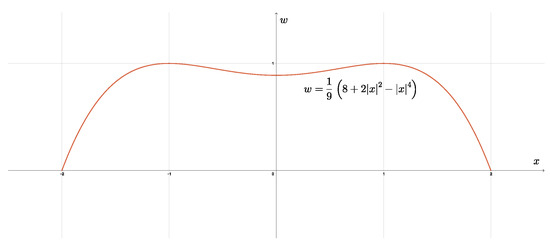
Figure 1. The graph of $w_m$ in the case $n=1$.

Then, we have $0\le w_m\left(x\right)\le 1$ whenever $\left|x\right|\le 2$ and $w_m\left(x\right)=1$ for $\left|x\right|=1$.

If $\mathsf{\Gamma }:]-\infty ,1[\to \mathbb{R}$ is the convex function defined by

$$\mathsf{\Gamma }\left(s\right)={\displaystyle \frac{s}{1-s}},$$

it turns out that

$${\mathsf{\Gamma }}^{\prime }\left(s\right)={\displaystyle \frac{1}{{(1-s)}^2}},\mathsf{\Gamma }\left(w_m\left(x\right)\right)={\displaystyle \frac{8+{2\left|x\right|}^2-{\left|x\right|}^4}{{(1-|x|}^2{)}^2}},{\mathsf{\Gamma }}^{\prime }\left(w_m\left(x\right)\right)={\displaystyle \frac{81}{{(1-|x|}^2{)}^4}}.$$

Now, define first $\widehat{f}:W_0^{1,2}\left(\mathsf{\Omega }\right)\to ]-\infty ,+\infty ]$ by

$$\widehat{f}\left(w\right)=\left\{\begin{array}{cc}{\displaystyle \frac{1}{2}{\int }_{\mathsf{\Omega }}{\left|Dw\right|}^{2}dx+{\int }_{\mathsf{\Omega }}\widehat{G}(x,w)dx}\hfill & \mathit{if}w<1\mathrm{a}.\mathrm{e}.\mathrm{in}\mathsf{\Omega },\hfill \\ +\infty \hfill & \mathit{otherwise},\hfill \end{array}\right.$$

where $\widehat{G}:\mathsf{\Omega }\times ]-\infty ,1[\to \mathbb{R}$ is the $C^{\infty }$-function defined by

$$\widehat{G}(x,s)={\displaystyle \frac{1}{2}}{s}^2{+(1-|x|}^2{)}^4\mathsf{\Gamma }\left(s\right)+\left[\mathsf{\Delta }{w}_m\left(x\right)-w_m\left(x\right)-81\right]s.$$

It is easily seen that

$$\begin{array}{c}\underset{\mathsf{\Omega }\times ]-\infty ,1[}{inf}\widehat{G}>-\infty ,\\ \underset{s\to -\infty }{lim}\widehat{G}(x,s)=\underset{s\to 1}{lim}\widehat{G}(x,s)=+\infty \mathit{whenever}\left|x\right|\ne 1,\end{array}$$

and that $\widehat{f}$ is lower semicontinuous, strictly convex, proper and coercive. Therefore $\widehat{f}$ has one and only one minimum point, which is just $w_m$, as

$$\begin{array}{c}{w}_m\in W_0^{1,2}\left(\mathsf{\Omega }\right)\cap W^{2,2}\left(\mathsf{\Omega }\right),\widehat{G}(x,w_m)\in L^1\left(\mathsf{\Omega }\right),D_s\widehat{G}(x,w_m)\in L^2\left(\mathsf{\Omega }\right),\\ -\mathsf{\Delta }{w}_m+D_s\widehat{G}(x,w_m)=0a.e.\mathrm{in}\mathsf{\Omega }.\end{array}$$

Let now $\nu :\mathbb{R}\to ]0,+\infty [$ be a $C^{\infty }$-function such that

$${\int }_{-\infty }^0{\left[\nu \left(s\right)\right]}^{1/2}ds=+\infty ,{\int }_0^{+\infty }{\left[\nu \left(s\right)\right]}^{1/2}ds=2^{-1/2}$$

and let $\psi :\mathbb{R}\to ]-\infty ,1[$ be the primitive of ${\left[2\nu \right]}^{1/2}$ such that $\psi \left(0\right)=0$. We have that

$$\underset{s\to -\infty }{lim}\psi \left(s\right)=-\infty ,\underset{s\to +\infty }{lim}\psi \left(s\right)=1$$

and that

$$w_m\in \left\{\psi \left(u\right):u\in {\mathcal{T}}_0^{1,2}\left(\mathsf{\Omega }\right),{\int }_{\mathsf{\Omega }}{\left[{\psi }^{\prime }\left(u\right)\right]}^2{\left|Du\right|}^{2}dx<+\infty \right\}\subseteq W_0^{1,2}\left(\mathsf{\Omega }\right).$$

Therefore, if we set $G(x,s)=\widehat{G}(x,\psi \left(s\right))$ and

$$L(x,s,\xi )={\nu \left(s\right)\left|\xi \right|}^2+G(x,s)={\displaystyle \frac{1}{2}}{\left[{\psi }^{\prime }\left(s\right)\right]}^2{\left|\xi \right|}^2+\widehat{G}(x,\psi \left(s\right)),$$

it turns out that L is of class $C^{\infty }$ on $\mathsf{\Omega }\times \mathbb{R}\times {\mathbb{R}}^n$ and that the assumptions of Theorem 1 are satisfied. In particular, hypotheses (L₁), (L^′₂), (L₃), (L_4,p) with $p=2$ and (L₅) hold. On the other hand, the functional

$$f\left(u\right)={\int }_{\mathsf{\Omega }}L(x,u,Du)dx$$

has one and only one minimum point $u_m\in {\mathcal{T}}_0^{1,2}\left(\mathsf{\Omega }\right)$, which is given by $u_m={\psi }^{-1}\left(w_m\right)$. Therefore, we have $u_m\in C^{\infty }(\mathsf{\Omega }\setminus \{\left|x\right|=1\left\}\right)$ and

$$\underset{y\to x}{lim}{u}_m\left(y\right)=+\infty \mathit{whenever}\left|x\right|=1,$$

whence

$$\underset{r\to 0}{lim}{\displaystyle \frac{1}{{\mathcal{L}}^n\left({\mathrm{B}}_r\left(x\right)\right)}}{\int }_{{\mathrm{B}}_r\left(x\right)}\left|\phi \left(u_m\right)\right|dx=+\infty \mathit{whenever}\left|x\right|=1,$$

for all $\phi \in \mathsf{\Phi }$. It follows that $\phi \left(u_m\right)\notin W_{loc}^{1,1}\left(\mathsf{\Omega }\right)$, for all $\phi \in \mathsf{\Phi }$ (see, e.g., (Theorem 3.77 of [21])).

Example  2.

Let $w_m:{\mathbb{R}}^n\to [0,1]$ be a $C^{\infty }$-function such that $w_m\left(x\right)=1$ whenever $\left|x\right|\le 1$ and $w_m\left(x\right)=0$ whenever $\left|x\right|\ge 2$. Let again $\mathsf{\Omega }=\left\{x\in {\mathbb{R}}^n:\left|x\right|<2\right\}$ and define first $\widehat{f}:W_0^{1,2}\left(\mathsf{\Omega }\right)\to \mathbb{R}$ by

$$\widehat{f}\left(w\right)={\displaystyle \frac{1}{2}}{\int }_{\mathsf{\Omega }}{\left|Dw\right|}^{2}dx+{\int }_{\mathsf{\Omega }}\widehat{G}(x,w)dx,$$

where $\widehat{G}:\mathsf{\Omega }\times \mathbb{R}\to \mathbb{R}$ is the $C^{\infty }$-function defined by

$$\widehat{G}(x,s)={\displaystyle \frac{1}{2}}{s}^2+\left[\mathsf{\Delta }{w}_m\left(x\right)-w_m\left(x\right)\right]s.$$

It is easily seen that

$$\underset{\mathsf{\Omega }\times \mathbb{R}}{inf}\widehat{G}>-\infty$$

and that $\widehat{f}$ is lower semicontinuous, strictly convex and coercive. Therefore $\widehat{f}$ has one and only one minimum point, which is just $w_m$. Moreover, if we set

$$D=\left\{u\in W_0^{1,2}\left(\mathsf{\Omega }\right):\underset{\mathsf{\Omega }}{\mathrm{ess}\sup }u<1\right\},$$

it turns out that

$$\underset{D}{inf}\widehat{f}=\underset{W_0^{1,2}\left(\mathsf{\Omega }\right)}{min}\widehat{f}.$$

Let now again ν and ψ be defined as in Example 1. We have

$$D\subseteq \left\{\psi \left(u\right):u\in {\mathcal{T}}_0^{1,2}\left(\mathsf{\Omega }\right),{\int }_{\mathsf{\Omega }}{\left[{\psi }^{\prime }\left(u\right)\right]}^2{\left|Du\right|}^{2}dx<+\infty \right\}\subseteq W_0^{1,2}\left(\mathsf{\Omega }\right).$$

Moreover, if we set $G(x,s)=\widehat{G}(x,\psi \left(s\right))$ and

$$L(x,s,\xi )={\nu \left(s\right)\left|\xi \right|}^2+G(x,s)={\displaystyle \frac{1}{2}}{\left[{\psi }^{\prime }\left(s\right)\right]}^2{\left|\xi \right|}^2+\widehat{G}(x,\psi \left(s\right)),$$

it turns out that L is of class $C^{\infty }$ on $\mathsf{\Omega }\times \mathbb{R}\times {\mathbb{R}}^n$ and that assumptions (L₁), (L^′₂), (L₃), and (L_4,p) with $p=2$ are satisfied. On the other hand, the functional

$$f\left(u\right)={\int }_{\mathsf{\Omega }}L(x,u,Du)dx$$

has no minimum point in ${\mathcal{T}}_0^{1,2}\left(\mathsf{\Omega }\right)$, because

$$\underset{{\mathcal{T}}_0^{1,2}\left(\mathsf{\Omega }\right)}{inf}f=\underset{W_0^{1,2}\left(\mathsf{\Omega }\right)}{min}\widehat{f},$$

but $w_m\ne \psi \left(u\right)$, for all $u\in {\mathcal{T}}_0^{1,2}\left(\mathsf{\Omega }\right)$. In this case, assumption (L₅) is not satisfied.

Remark  2.

As already observed in the Introduction, after proving the lower semicontinuity and the coercivity of the functional in a suitable functional setting, the existence of a minimum follows in a standard way. More precisely, (L₁)–(L₃) are the natural assumptions to ensure the lower semicontinuity, while (L_4,p) and (L₅) imply the coercivity. Assumption (L^′₂) is the typical stronger variant of (L₂), designed to obtain the strong precompactness of the minimizing sequences.

Let us point out that (L₅) is essential for the coercivity, according to Example 2, in which (L₅) is not satisfied and the functional admits no minimum.

This is the basic set of assumptions for minimization. In the next sections, we will consider other assumptions either to ensure that each minimum is more regular or to prove that it satisfies a suitable form of the Euler–Lagrange equation.

Remark  3.

Let us point out that, under the assumptions (L₁), (L^′₂), (L₃), (L_4,p) and (L₅), it may happen that the functional admits no minimum in $W_0^{1,p}\left(\mathsf{\Omega }\right)$. Actually, by Example 1, the situation is even worse. It may happen that each minimum u satisfies $\phi \left(u\right)\notin W_{loc}^{1,1}\left(\mathsf{\Omega }\right)$, for all $\phi \in \mathsf{\Phi }$. Of course, this implies that $u\notin W_0^{1,p}\left(\mathsf{\Omega }\right)$, but even that the minimization cannot be reduced to a Sobolev setting “up to diffeomorphism”.

8. Regularity of Minima

Throughout this section, we assume that $\mathsf{\Omega }$ is a bounded and open subset of ${\mathbb{R}}^n$, that $1\le p<\infty$, and that

$$L:\mathsf{\Omega }\times \mathbb{R}\times {\mathbb{R}}^n⟶\mathbb{R}$$

satisfies (L₁) and $L(x,0,0)\in L^1\left(\mathsf{\Omega }\right)$.

Theorem  8.

Assume there exist $\psi \in \mathsf{\Phi }$, $\alpha \in L^1\left(\mathsf{\Omega }\right)$ and a negligible subset N of Ω such that

$$L(x,s,\xi )\ge |{\psi }^{\prime }{\left(s\right)|}^p{\left|\xi \right|}^p-\alpha \left(x\right),$$

for all $(x,s,\xi )\in (\mathsf{\Omega }\setminus N)\times \mathbb{R}\times {\mathbb{R}}^n$. Let $u\in {\mathcal{T}}_0^{1,p}\left(\mathsf{\Omega }\right)$ be such that

$${\int }_{\mathsf{\Omega }}L(x,u,Du)dx\le {\int }_{\mathsf{\Omega }}L(x,w,Dw)dx\mathit{for}\mathit{all}w\in {\mathcal{T}}_0^{1,p}\left(\mathsf{\Omega }\right).$$

Then there exists $\phi \in \mathsf{\Phi }$ such that $\phi \left(u\right)\in W_0^{1,p}\left(\mathsf{\Omega }\right)$.

Proof. 

Of course, assumption (L₃) also is satisfied. If we set $\phi ={\psi }^{-1}$, we have

$$L^{\phi }(x,s,\xi )\ge {\left|\xi \right|}^p-\alpha \left(x\right).$$

Since

$${\int }_{\mathsf{\Omega }}{L}^{\phi }(x,u_{\phi },D{u}_{\phi })dx\le {\int }_{\mathsf{\Omega }}{L}^{\phi }(x,0,0)dx<+\infty ,$$

it follows that $D{u}_{\phi }\in L^p(\mathsf{\Omega };{\mathbb{R}}^n)$, whence $u_{\phi }\in W_0^{1,p}\left(\mathsf{\Omega }\right)$, as $\mathsf{\Omega }$ is bounded. □

Theorem  9.

Assume that $1\le p<n$ and that there exist $\psi \in \mathsf{\Phi }$, $\alpha \in L^r\left(\mathsf{\Omega }\right)$, ${\beta }_1\in L^t\left(\mathsf{\Omega }\right)$, ${\beta }_2\in \mathbb{R}$ and a negligible subset N of Ω such that

$$\begin{array}{c}r>{\displaystyle \frac{n}{p}},t>{\displaystyle \frac{n}{p}},\\ L(x,s,\xi )\ge |{\psi }^{\prime }{\left(s\right)|}^p{\left|\xi \right|}^p-\alpha \left(x\right),\\ L(x,s,0)\le \alpha \left(x\right)+{\beta }_1{\left(x\right)\left|\psi \left(s\right)\right|}^{{\displaystyle \frac{p^{*}}{t^{\prime }}}}+{\beta }_2{\left|\psi \left(s\right)\right|}^{p^{*}},\end{array}$$

for all $(x,s,\xi )\in (\mathsf{\Omega }\setminus N)\times \mathbb{R}\times {\mathbb{R}}^n$, where $p^{*}={\displaystyle \frac{np}{n-p}}$. Let $u\in {\mathcal{T}}_0^{1,p}\left(\mathsf{\Omega }\right)$ be such that

$${\int }_{\mathsf{\Omega }}L(x,u,Du)dx\le {\int }_{\mathsf{\Omega }}L(x,w,Dw)dx\mathit{for}\mathit{all}w\in {\mathcal{T}}_0^{1,p}\left(\mathsf{\Omega }\right).$$

Then we have $u\in W_0^{1,p}\left(\mathsf{\Omega }\right)\cap L^{\infty }\left(\mathsf{\Omega }\right)$.

Proof. 

If we set $\phi ={\psi }^{-1}$, we have

$$L^{\phi }(x,s,\xi )\ge {\left|\xi \right|}^p-\alpha \left(x\right),L^{\phi }(x,s,0)\le \alpha \left(x\right)+{\beta }_1{\left(x\right)\left|s\right|}^{{\displaystyle \frac{p^{*}}{t^{\prime }}}}+{\beta }_2{\left|s\right|}^{p^{*}}.$$

As before, we deduce that $u_{\phi }\in W_0^{1,p}\left(\mathsf{\Omega }\right)$. Then, from Theorem A1 in the Appendix A we infer that $u_{\phi }\in L^{\infty }\left(\mathsf{\Omega }\right)$, whence $u\in W_0^{1,p}\left(\mathsf{\Omega }\right)\cap L^{\infty }\left(\mathsf{\Omega }\right)$. □

It is easily seen that also the assumptions of the previous results are invariant by diffeomorphism.

Remark  4.

It ${\displaystyle \frac{n}{p}}<t<\tau <\infty$ and $\beta \in L^{\tau }\left(\mathsf{\Omega }\right)$, then we have

$${\beta \left(x\right)\left|s\right|}^{{\displaystyle \frac{p^{*}}{{\tau }^{\prime }}}}={\beta \left(x\right)\left|s\right|}^{{\displaystyle \frac{t-1}{\tau }}{p}^{*}}{\left|s\right|}^{{\displaystyle \frac{\tau -t}{\tau }}{p}^{*}}\le {\displaystyle \frac{t}{\tau }}{\left|\beta \left(x\right)\right|}^{{\displaystyle \frac{\tau }{t}}}{\left|s\right|}^{{\displaystyle \frac{p^{*}}{t^{\prime }}}}+{\displaystyle \frac{\tau -t}{\tau }}{\left|s\right|}^{p^{*}}$$

with ${\left|\beta \left(x\right)\right|}^{{\displaystyle \frac{\tau }{t}}}\in L^t\left(\mathsf{\Omega }\right)$. Therefore, intermediate powers ${\left|s\right|}^{\gamma }$, with ${\displaystyle \frac{p^{*}}{t^{\prime }}}<\gamma <p^{*}$, can be estimated in terms of ${\left|s\right|}^{{\displaystyle \frac{p^{*}}{t^{\prime }}}}$ and ${\left|s\right|}^{p^{*}}$, with the correct summability of the coefficients.

9. Euler–Lagrange Equation

Throughout this section, we assume that $\mathsf{\Omega }$ is an open subset of ${\mathbb{R}}^n$, that $1\le p<\infty$ and that

$$L:\mathsf{\Omega }\times \mathbb{R}\times {\mathbb{R}}^n⟶\mathbb{R}$$

is a function such that the following hold:

(L_6,p)

There exists a negligible subset N of Ω such that we have the following:

• For every $(s,\xi )\in \mathbb{R}\times {\mathbb{R}}^n$, the function $L(·,s,\xi )$ is measurable on Ω;
• For every $x\in \mathsf{\Omega }\setminus N$, the function $L(x,·,·)$ is of class $C^1$ on $\mathbb{R}\times {\mathbb{R}}^n$;
• For every $S>0$, there exist ${\alpha }_S^{\left(0\right)}\in L_{loc}^1\left(\mathsf{\Omega }\right)$, ${\alpha }_S^{\left(1\right)}\in L_{loc}^{p^{\prime }}\left(\mathsf{\Omega }\right)$ and ${\beta }_S\in L_{loc}^{\infty }\left(\mathsf{\Omega }\right)$ such that

  $$\begin{array}{cccc}& \left|D_{\xi }L(x,s,\xi )\right|\hfill & & \le {\alpha }_S^{\left(1\right)}\left(x\right)+{\beta }_S\left(x\right){\left|\xi \right|}^{p-1},\hfill \\ & \left|D_{s}L(x,s,\xi )\right|\hfill & & \le {\alpha }_S^{\left(0\right)}\left(x\right)+{\beta }_S\left(x\right){\left|\xi \right|}^p,\hfill \end{array}$$
  for all $(x,s,\xi )\in (\mathsf{\Omega }\setminus N)\times \mathbb{R}\times {\mathbb{R}}^n$ with $\left|s\right|\le S$.

As usual, it follows that $L^{\phi }$ also satisfies (L_6,p), for all $\phi \in \mathsf{\Phi }$.

Let $L_c^{\infty }\left(\mathsf{\Omega }\right)$ denote the set of $v^{\prime }s$ in $L^{\infty }\left(\mathsf{\Omega }\right)$ vanishing a.e. outside some compact subset of $\mathsf{\Omega }$. Then, following an idea of [22], for every $u\in {\mathcal{T}}_0^{1,p}\left(\mathsf{\Omega }\right)$, we denote by $V_u$ the linear space of $v^{\prime }s$ in $W_0^{1,p}\left(\mathsf{\Omega }\right)\cap L_c^{\infty }\left(\mathsf{\Omega }\right)$ such that u is essentially bounded on $\left\{x\in \mathsf{\Omega }:v\left(x\right)\ne 0\right\}$. For instance, if $v\in W_0^{1,p}\left(\mathsf{\Omega }\right)\cap L_c^{\infty }\left(\mathsf{\Omega }\right)$ and $\vartheta \in W^{1,\infty }\left(\mathbb{R}\right)\cap L_c^{\infty }\left(\mathbb{R}\right)$, then $\vartheta \left(u\right)v\in V_u$.

For every $u\in {\mathcal{T}}_0^{1,p}\left(\mathsf{\Omega }\right)$, every $\phi \in \mathsf{\Phi }$ and every measurable function v, we set also

$$v_{\phi ,u}={\left({\phi }^{-1}\right)}^{\prime }\left(u\right)v={\displaystyle \frac{v}{{\phi }^{\prime }\left(u_{\phi }\right)}}.$$

The next assertions are easily proved.

Proposition  3.

For every $u\in {\mathcal{T}}_0^{1,p}\left(\mathsf{\Omega }\right)$, $v\in V_u$ and $\phi \in \mathsf{\Phi }$, the following facts hold:

(a) 

We have

$$\begin{array}{c}u+v\in {\mathcal{T}}_0^{1,p}\left(\mathsf{\Omega }\right),L(x,u+v,D(u+v))-L(x,u,Du)\in L^1\left(\mathsf{\Omega }\right),\\ D_{\xi }L(x,u,Du)·Dv+D_{s}L(x,u,Du)v\in L^1\left(\mathsf{\Omega }\right);\end{array}$$

(b) 

We have $v_{\phi ,u}\in V_{u_{\phi }}$ and the linear map $\left\{v\mapsto v_{\phi ,u}\right\}$ is a bijection of $V_u$ onto $V_{u_{\phi }}$;

(c) 

We have

$$\begin{array}{c}{D}_{\xi }{L}^{\phi }(x,u_{\phi },D{u}_{\phi })·D{u}_{\phi }=D_{\xi }L(x,u,Du)·Du,\\ D_{\xi }{L}^{\phi }(x,u_{\phi },D{u}_{\phi })·D{v}_{\phi ,u}+D_s{L}^{\phi }(x,u_{\phi },D{u}_{\phi })v_{\phi ,u}\\ =D_{\xi }L(x,u,Du)·Dv+D_{s}L(x,u,Du)v\end{array}$$

a.e. in Ω.

Theorem  10.

Let $u\in {\mathcal{T}}_0^{1,p}\left(\mathsf{\Omega }\right)$ be such that

$${\int }_{\mathsf{\Omega }}\left[L(x,u+v,D(u+v\left)\right)-L(x,u,Du)\right]dx\ge 0\mathit{for}\mathit{all}v\in V_u.$$

Then we have

$${\int }_{\mathsf{\Omega }}\left[D_{\xi }L(x,u,Du)·Dv+D_{s}L(x,u,Du)v\right]dx=0\mathit{for}\mathit{all}v\in V_u.$$

Proof. 

It easily follows from Lebesgue’s Theorem. □

Now, for every $u\in {\mathcal{T}}_0^{1,p}\left(\mathsf{\Omega }\right)$ and $\psi \in \mathsf{\Phi }$, we define the linear space

$$V_u^{\psi }=\left\{{\displaystyle \frac{w}{{\psi }^{\prime }\left(u\right)}}:w\in W_0^{1,p}\left(\mathsf{\Omega }\right)\cap L_c^{\infty }\left(\mathsf{\Omega }\right)\right\}.$$

We remark that ${\displaystyle \frac{w}{{\psi }^{\prime }\left(T_h\left(u\right)\right)}}\in W_0^{1,p}\left(\mathsf{\Omega }\right)\cap L_c^{\infty }\left(\mathsf{\Omega }\right)$, for all $h>0$, and we set

$$D\left({\displaystyle \frac{w}{{\psi }^{\prime }\left(u\right)}}\right)=\underset{h\to +\infty }{lim}D\left({\displaystyle \frac{w}{{\psi }^{\prime }\left(T_h\left(u\right)\right)}}\right)\mathrm{a}.\mathrm{e}.\mathrm{in}\mathsf{\Omega }.$$

Moreover, if $v={\displaystyle \frac{w}{{\psi }^{\prime }\left(u\right)}}\in V_u^{\psi }$, it turns out that

$$v_{\phi ,u}={\displaystyle \frac{1}{{\phi }^{\prime }\left(u_{\phi }\right)}}{\displaystyle \frac{w}{{\psi }^{\prime }\left(u\right)}}={\displaystyle \frac{w}{{\psi }^{\prime }\left(\phi \left(u_{\phi }\right)\right){\phi }^{\prime }\left(u_{\phi }\right)}}={\displaystyle \frac{w}{{(\psi \circ \phi )}^{\prime }\left(u_{\phi }\right)}}.$$

Therefore, we have $v_{\phi ,u}\in V_{u_{\phi }}^{\psi \circ \phi }$ for all $v\in V_u^{\psi }$ and the linear map $\left\{v\mapsto v_{\phi ,u}\right\}$ is a bijection of $V_u^{\psi }$ onto $V_{u_{\phi }}^{\psi \circ \phi }$. As before, we also have

$$\begin{array}{c}{D}_{\xi }{L}^{\phi }(x,u_{\phi },D{u}_{\phi })·D{v}_{\phi ,u}+D_s{L}^{\phi }(x,u_{\phi },D{u}_{\phi })v_{\phi ,u}\hfill \\ \hspace{1em}\hspace{1em}\hspace{1em}\hspace{1em}\hspace{1em}\hspace{1em}\hspace{1em}\hspace{1em}\hspace{1em}\hspace{1em}\hspace{1em}\hspace{1em}\hspace{1em}\hspace{1em}\hspace{1em}\hspace{1em}\hspace{1em}=D_{\xi }L(x,u,Du)·Dv+D_{s}L(x,u,Du)v\end{array}$$

a.e. in $\mathsf{\Omega }$, for all $u\in {\mathcal{T}}_0^{1,p}\left(\mathsf{\Omega }\right)$, $\phi ,\psi \in \mathsf{\Phi }$ and $v\in V_u^{\psi }$.

Theorem  11.

Let $u\in {\mathcal{T}}_0^{1,p}\left(\mathsf{\Omega }\right)$ be such that

$$\begin{array}{c}{D}_{\xi }L(x,u,Du)·Du\in L_{loc}^1\left(\mathsf{\Omega }\right),\\ {\int }_{\mathsf{\Omega }}\left[D_{\xi }L(x,u,Du)·Dv+D_{s}L(x,u,Du)v\right]dx=0\mathit{for}\mathit{all}v\in V_u.\end{array}$$

Then we have

$$\begin{array}{c}{\int }_{\mathsf{\Omega }}{\left[D_{\xi }L(x,u,Du)·Dv+D_{s}L(x,u,Du)v\right]}^{+}dx\hfill \\ \hspace{1em}={\int }_{\mathsf{\Omega }}{\left[D_{\xi }L(x,u,Du)·Dv+D_{s}L(x,u,Du)v\right]}^{-}dx\\ \hspace{1em}\hspace{1em}\hspace{1em}\hspace{1em}\hspace{1em}\hspace{1em}\hspace{1em}\hspace{1em}\hspace{1em}\hspace{1em}\hspace{1em}\hspace{1em}\hspace{1em}\hspace{1em}\hspace{1em}\hspace{1em}\hspace{1em}\hspace{1em}\hspace{1em}\hspace{1em}\hspace{1em}\hspace{1em}\hspace{1em}\hspace{1em}\hspace{1em}\mathit{for}\mathit{all}\psi \in \mathsf{\Phi }\mathit{and}\mathit{all}v\in V_u^{\psi }\end{array}$$

(both sides could be $+\infty$).

Proof. 

Let us first treat the case $\psi \left(s\right)=s$, namely $v\in V_u^{\mathrm{Id}}=W_0^{1,p}\left(\mathsf{\Omega }\right)\cap L_c^{\infty }\left(\mathsf{\Omega }\right)$. In this case the argument is an adaptation of the proof of (Theorem 4.7 of [23]). Assume, for instance, that ${\left[D_{\xi }L(x,u,Du)·Dv+D_{s}L(x,u,Du)v\right]}^{-}\in L^1\left(\mathsf{\Omega }\right)$. Let $\vartheta :\mathbb{R}\to [0,1]$ be a $C^{\infty }$-function such that $\vartheta \left(s\right)=1$ whenever $\left|s\right|\le 1$, and $\vartheta \left(s\right)=0$ whenever $\left|s\right|\ge 2$. Then, $\vartheta (u/k)v\in V_u$ and we have

$$\begin{array}{c}{\int }_{\mathsf{\Omega }}\vartheta \left({\displaystyle \frac{u}{k}}\right)\left[D_{\xi }L(x,u,Du)·Dv+D_{s}L(x,u,Du)v\right]dx\hfill \\ \hspace{1em}\hspace{1em}\hspace{1em}\hspace{1em}\hspace{1em}\hspace{1em}\hspace{1em}\hspace{1em}\hspace{1em}\hspace{1em}\hspace{1em}\hspace{1em}\hspace{1em}\hspace{1em}\hspace{1em}=-{\displaystyle \frac{1}{k}}{\int }_{\mathsf{\Omega }}v{\vartheta }^{\prime }\left({\displaystyle \frac{u}{k}}\right)D_{\xi }L(x,u,Du)·Dudx.\end{array}$$

(7)

Since

$$\begin{array}{c}\vartheta \left({\displaystyle \frac{u}{k}}\right)\left[D_{\xi }L(x,u,Du)·Dv+D_{s}L(x,u,Du)v\right]\\ \ge -{\left[D_{\xi }L(x,u,Du)·Dv+D_{s}L(x,u,Du)v\right]}^{-},\\ \underset{k}{lim}{\displaystyle \frac{1}{k}}{\int }_{\mathsf{\Omega }}v{\vartheta }^{\prime }\left({\displaystyle \frac{u}{k}}\right)D_{\xi }L(x,u,Du)·Dudx=0,\end{array}$$

from Fatou’s Lemma, we infer that

$${\int }_{\mathsf{\Omega }}\left[D_{\xi }L(x,u,Du)·Dv+D_{s}L(x,u,Du)v\right]dx\le 0,$$

whence ${\left[D_{\xi }L(x,u,Du)·Dv+D_{s}L(x,u,Du)v\right]}^{+}\in L^1\left(\mathsf{\Omega }\right)$. Coming back to (7), from Lebesgue’s Theorem, we conclude that

$${\int }_{\mathsf{\Omega }}\left[D_{\xi }L(x,u,Du)·Dv+D_{s}L(x,u,Du)v\right]dx=0.$$

If ${\left[D_{\xi }L(x,u,Du)·Dv+D_{s}L(x,u,Du)v\right]}^{+}\in L^1\left(\mathsf{\Omega }\right)$, the argument is similar.

Consider now the general case. Let $\psi \in \mathsf{\Phi }$ and let $v\in V_u^{\psi }$. If we set $\phi ={\psi }^{-1}$, it follows that $v_{\phi ,u}\in V_{u_{\phi }}^{\mathrm{Id}}$, while

$$\begin{array}{c}{D}_{\xi }{L}^{\phi }(x,u_{\phi },D{u}_{\phi })·D{u}_{\phi }=D_{\xi }L(x,u,Du)·Du\in L_{loc}^1\left(\mathsf{\Omega }\right),\\ {\int }_{\mathsf{\Omega }}\left[D_{\xi }{L}^{\phi }(x,u_{\phi },D{u}_{\phi })·Dw+D_s{L}^{\phi }(x,u_{\phi },D{u}_{\phi })w\right]dx=0\mathrm{for}\mathrm{all}w\in V_{u_{\phi }}.\end{array}$$

From the previous step, we infer that

$$\begin{array}{c}{\int }_{\mathsf{\Omega }}{\left[D_{\xi }{L}^{\phi }(x,u_{\phi },D{u}_{\phi })·D{v}_{\phi ,u}+D_s{L}^{\phi }(x,u_{\phi },D{u}_{\phi })v_{\phi ,u}\right]}^{+}dx\hfill \\ \hspace{1em}\hspace{1em}\hspace{1em}\hspace{1em}\hspace{1em}\hspace{1em}\hspace{1em}\hspace{1em}\hspace{1em}={\int }_{\mathsf{\Omega }}{\left[D_{\xi }{L}^{\phi }(x,u_{\phi },D{u}_{\phi })·D{v}_{\phi ,u}+D_s{L}^{\phi }(x,u_{\phi },D{u}_{\phi })v_{\phi ,u}\right]}^{-}dx\end{array}$$

and the assertion follows. □

Remark  5.

If $\left\{\xi \mapsto L(x,s,\xi )-L(x,s,0)\right\}$ is positively homogeneous of degree p and we have

$$L(x,s,\xi )-L(x,s,0)\ge -\underline{\alpha }\left(x\right),L(x,s,0)\ge -\underline{\alpha }\left(x\right),$$

for some $\underline{\alpha }\in L^1\left(\mathsf{\Omega }\right)$, then it follows that

$$-p\underline{\alpha }\le p\left[L(x,u,Du)-L(x,u,0)\right]=D_{\xi }L(x,u,Du)·Du\le pL(x,u,Du)+p\underline{\alpha }.$$

Therefore, the assumption

$$D_{\xi }L(x,u,Du)·Du\in L_{loc}^1\left(\mathsf{\Omega }\right)$$

is implied by $L(x,u,Du)\in L^1\left(\mathsf{\Omega }\right)$.

References

- Buttazzo, G. Semicontinuity, Relaxation and Integral Representation in the Calculus of Variations; Pitman Research Notes in Mathematics Series; Longman Scientific & Technical: Harlow, UK, 1989; Volume 207. [Google Scholar]
- Aharouch, L.; Bennouna, J.; Bouajaja, A. Existence and regularity of minima of an integral functional in unbounded domain. Aust. J. Math. Anal. Appl. 2015, 12, 1–16. [Google Scholar]
- Aharouch, L.; Bennouna, J.; Bouajaja, A. Minima of some integral functional: Existence and regularity. Nonlinear Dyn. Syst. Theory 2016, 16, 335–349. [Google Scholar]
- Arcoya, D.; Boccardo, L. A class of integral functionals with a -minimum. Atti Accad. Naz. Lincei Rend. Lincei Mat. Appl. 2022, 33, 535–551. [Google Scholar]
- Boccardo, L.; Croce, G.; Orsina, L. minima of noncoercive functionals. Atti Accad. Naz. Lincei Rend. Lincei Mat. Appl. 2011, 22, 513–523. [Google Scholar]
- Boccardo, L.; Orsina, L. Existence and regularity of minima for integral functionals noncoercive in the energy space. Ann. Sc. Norm. Super.-Pisa-Cl. Sci. 1997, 25, 95–130. [Google Scholar]
- Mercaldo, A. Existence and boundedness of minimizers of a class of integral functionals. Boll. dell’Unione Mat. Ital. 2003, 6, 125–139. [Google Scholar]
- Marsden, J.E.; Hughes, T.J.R. Mathematical Foundations of Elasticity; Dover Publications, Inc.: New York, NY, USA, 1994. [Google Scholar]
- Milnor, J.W. Topology from the Differentiable Viewpoint; Princeton Landmarks in Mathematics; Princeton University Press: Princeton, NJ, USA, 1997. [Google Scholar]
- Kazdan, J.L.; Kramer, R.J. Invariant criteria for existence of solutions to second-order quasilinear elliptic equations. Commun. Pure Appl. Math. 1978, 31, 619–645. [Google Scholar] [CrossRef]
- Bénilan, P.; Boccardo, L.; Gallouët, T.; Gariepy, R.; Pierre, M.; Vázquez, J.L. An L1-theory of existence and uniqueness of solutions of nonlinear elliptic equations. Ann. Sc. Norm. Super.-Pisa-Cl. Sci. 1995, 22, 241–273. [Google Scholar]
- Boccardo, L.; Gallouët, T.; Orsina, L. Existence and uniqueness of entropy solutions for nonlinear elliptic equations with measure data. Ann. L’Inst. Henri Poincaré (C) Anal. Non Linéaire 1996, 13, 539–551. [Google Scholar] [CrossRef]
- Dal Maso, G.; Murat, F.; Orsina, L.; Prignet, A. Renormalized solutions of elliptic equations with general measure data. Ann. Sc. Norm. Super.-Pisa-Cl. Sci. 1999, 28, 741–808. [Google Scholar]
- Struwe, M. Variational Methods; Ergebnisse der Mathematik und Ihrer Grenzgebiete; Springer: Berlin/Heidelberg, Germany, 2008; Volume 34. [Google Scholar]
- Boccardo, L.; Gallouet, T. Compactness of minimizing sequences. Nonlinear Anal. 2016, 137, 213–221. [Google Scholar] [CrossRef]
- Brezis, H. Convergence in D′ and in L1 under strict convexity. In Boundary Value Problems for Partial Differential Equations and Applications; Lions, J.L., Baiocchi, C., Eds.; RMA Research Notes in Applied Mathematics; Masson: Paris, France, 1993; Volume 29, pp. 43–52. [Google Scholar]
- Visintin, A. Strong convergence results related to strict convexity. Commun. Partial Differ. Equ. 1984, 9, 439–466. [Google Scholar] [CrossRef]
- Solferino, V.; Squassina, M. Diffeomorphism-invariant properties for quasi-linear elliptic operators. J. Fixed Point Theory Appl. 2012, 11, 137–157. [Google Scholar] [CrossRef][Green Version]
- Ioffe, A.D. On lower semicontinuity of integral functionals. II. SIAM J. Control Optim. 1977, 15, 991–1000. [Google Scholar] [CrossRef]
- Degiovanni, M.; Marzocchi, M. Multiple critical points for symmetric functionals without upper growth condition on the principal part. Symmetry 2021, 13, 898. [Google Scholar] [CrossRef]
- Ambrosio, L.; Fusco, N.; Pallara, D. Functions of Bounded Variation and Free Discontinuity Problems; Oxford Mathematical Monographs; The Clarendon Press Oxford University Press: New York, NY, USA, 2000. [Google Scholar]
- Degiovanni, M.; Zani, S. Euler equations involving nonlinearities without growth conditions. Potential Anal. 1996, 5, 505–512. [Google Scholar] [CrossRef]
- Pellacci, B.; Squassina, M. Unbounded critical points for a class of lower semicontinuous functionals. J. Differ. Equ. 2004, 201, 25–62. [Google Scholar] [CrossRef]
- Ladyzhenskaya, O.A.; Ural’tseva, N.N. Linear and Quasilinear Elliptic Equations; Academic Press: New York, NY, USA, 1968. [Google Scholar]
- Cianchi, A. Boundedness of solutions to variational problems under general growth conditions. Commun. Partial Differ. Equ. 1997, 22, 1629–1646. [Google Scholar]
- Boccardo, L.; Giachetti, D. Alcune osservazioni sulla regolarità delle soluzioni di problemi fortemente non lineari e applicazioni. Ric. Mat. 1985, 34, 309–323. [Google Scholar]
- Giachetti, D.; Porzio, M.M. Local regularity results for minima of functionals of the calculus of variation. Nonlinear Anal. 2000, 39, 463–482. [Google Scholar] [CrossRef]
- Gilbarg, D.; Trudinger, N.S. Elliptic Partial Differential Equations of Second Order; Classics in Mathematics; Springer: Berlin/Heidelberg, Germany, 2001. [Google Scholar]
- Stampacchia, G. Le problème de Dirichlet pour les équations elliptiques du second ordre à coefficients discontinus. Ann. Inst. Fourier (Grenoble) 1965, 15, 189–258. [Google Scholar] [CrossRef]
Disclaimer/Publisher’s Note: The statements, opinions and data contained in all publications are solely those of the individual author(s) and contributor(s) and not of MDPI and/or the editor(s). MDPI and/or the editor(s) disclaim responsibility for any injury to people or property resulting from any ideas, methods, instructions or products referred to in the content. |
© 2025 by the authors. Licensee MDPI, Basel, Switzerland. This article is an open access article distributed under the terms and conditions of the Creative Commons Attribution (CC BY) license (https://creativecommons.org/licenses/by/4.0/).