Learning the Hybrid Nonlocal Self-Similarity Prior for Image Restoration

Abstract

As an immensely important characteristic of natural images, the nonlocal self-similarity (NSS) prior has demonstrated great promise in a variety of inverse problems. Unfortunately, most current methods utilize either the internal or the external NSS prior learned from the degraded image or training images. The former is inevitably disturbed by degradation, while the latter is not adapted to the image to be restored. To mitigate such problems, this work proposes to learn a hybrid NSS prior from both internal images and external training images and employs it in image restoration tasks. To achieve our aims, we first learn internal and external NSS priors from the measured image and high-quality image sets, respectively. Then, with the learned priors, an efficient method, involving only singular value decomposition (SVD) and a simple weighting method, is developed to learn the HNSS prior for patch groups. Subsequently, taking the learned HNSS prior as the dictionary, we formulate a structural sparse representation model with adaptive regularization parameters called HNSS-SSR for image restoration, and a general and efficient image restoration algorithm is developed via an alternating minimization strategy. The experimental results indicate that the proposed HNSS-SSR-based restoration method exceeds many existing competition algorithms in PSNR and SSIM values.

1. Introduction

Along with the advancement of various optical technologies and sensors, images have become one of the most important carriers of information. Unfortunately, image degradation is inevitable during acquisition, transmission, and storage because of defects in the imaging system and interference from various external factors. Therefore, image restoration, which strives to reconstruct the underlying uncorrupted image $\mathit{x}$ from the corrupted measurement $\mathit{y}$, is essential in a lot of fields of science and engineering. In general, the image degradation process is modeled as:

$$\begin{array}{c}\hfill \mathit{y}=\mathsf{\Phi }\mathit{x}+\mathit{v},\end{array}$$

(1)

where $\mathsf{\Phi }$ denotes the degradation operator and $\mathit{v}$ represents the white Gaussian noise. In Equation (1), different settings of $\mathsf{\Phi }$ correspond to different image restoration problems. To be specific, when $\mathsf{\Phi }$ is an identity matrix, Equation (1) becomes image denoising [1]; when $\mathsf{\Phi }$ is a blurring matrix, Equation (1) converts to image deblurring [2,3]; and when $\mathsf{\Phi }$ is a random projection matrix, Equation (1) denotes image compressive sensing [4,5].

As image restoration in Equation (1) is a typically ill-posed linear inverse problem, an image prior is often required to constrain the solution space. Specifically, from the standpoint of maximum a posteriori (MAP) estimation, the latent high-quality image can be inferred by solving the following regularization problem [2]:

$$\begin{array}{c}\hfill \widehat{\mathit{x}}=\underset{\mathit{x}}{argmin}{\parallel \mathit{y}-\mathsf{\Phi }\mathit{x}\parallel }_2^2+\eta \mathsf{\Psi }\left(\mathit{x}\right),\end{array}$$

(2)

where ${\parallel ·\parallel }_2^2$ denotes the $l_2$-norm, ${\parallel \mathit{y}-\mathsf{\Phi }\mathit{x}\parallel }_2^2$ is the fidelity term associated with Gaussian noise, $\mathsf{\Psi }\left(\mathit{x}\right)$ is the regularization term that relies on the image prior, and $\eta$ is employed to balance these two terms.

Due to the curse of dimensionality, it is almost impossible to model the whole image. A remedy is to use the image patch as the basic unit of modeling [6,7]. Thus, over the past few decades, the patch-based prior has been extensively studied and has achieved favorable image restoration performance, such as patch-based sparse representation [8,9,10,11,12,13] and patch-based image modeling [6,14,15,16]. Recently, deep learning has also been adopted to learn image priors in a supervised manner and has spawned promising results in various image restoration applications [17,18,19,20,21,22]. Both the model-based and deep learning-based approaches mentioned above, however, are dedicated to mining the local properties of images, whose performance is restricted by largely neglecting the self-similarity and nonlocal properties of images [1,23,24]. In addition, deep learning methods require a training set consisting of extensive degraded/high quality image pairs for supervised learning, which renders them difficult to apply or causes undesirable artifacts in some tasks, such as medical imaging and remote sensing [25,26].

As we all know, natural images have rich self-repeating structures in nonlocal regions, i.e., the so-called nonlocal self-similarity (NSS) prior [27,28]. Compared to the patch-based prior, the NSS prior enables us to cluster together nonlocal patches with similar patterns over the whole image and use such similar patch groups as the basic unit for restoration, which is especially helpful for recovering image structures [27,28,29], such as textures and edges. Given the great success of the nonlocal means (NLM) [27] method, a series of NSS prior-based methods have been developed successively and have shown impressive restoration effects. These approaches can be broadly summarized into three clusters, i.e., filter-based methods [27,29,30], patch group-based sparse representation methods [4,23,31,32,33,34,35,36,37,38], and low-rank approximation-based methods [2,39,40,41,42,43,44]. Apart from focusing on the internal NSS prior of the corrupted image, some recent approaches have paid attention to exploiting the external NSS prior learned from high-quality natural images [28,45,46]. For example, Xu et al. [28] developed a patch group prior-based denoising (PGPD) method for learning dictionaries from the natural image corpus. Liu et al. [46] formulated a external NSS prior-based group sparsity mixture model for image denoising. Although the aforementioned NSS prior-based methods have shown their potential in recovering image structures, exploiting the internal NSS of the observed image often suffers from overfitting data corruption [5], while the external NSS prior learned from training images is not well-adapted to the image to be recovered [47].

To rectify the weakness of using a single NSS prior, some more recent works proposed to jointly utilize internal and external NSS priors [1,3,5,7,24,26,48,49]. For instance, Zha et al. [1] developed a denoising method based on sparse residuals by using an external NSS prior. Liu et al. [49] proposed a group sparse representation-based super-resolution algorithm to leverage internal and external correlations. Zha et al. [24] proposed to simultaneously use internal and external NSS priors for image restoration. Yuan et al. [3] formulated a joint group dictionary-based structural sparse model for image restoration. Zha et al. [5] developed a hybrid structural sparsification error model to jointly exploit internal and external NSS priors. Yuan et al. [7] suggested the joint use of a low-rank prior and an external NSS prior. These methods have led to promising restoration results, since the complementary information of internal and external NSS priors is exploited.

Unlike the above works, in this paper, we propose to learn a hybrid NSS (HNSS) prior for image restoration. In particular, most of existing works mainly concentrate their attention on how to jointly utilize two priors, i.e., internal and external NSS priors, while this work focuses on developing a new paradigm to learn one HNSS prior from both the internal degraded and external natural image sets and applies the learned prior to image restoration. It can be seen that the technical route of our proposed method is quite different from the above existing works. The flowchart of our method is presented in Figure 1. To the best of our knowledge, how to learn an HNSS prior remains an unsolved problem, and this paper thus takes a stab at it. We summarize the main contributions as follows:

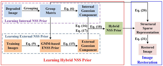
Figure 1. The flowchart of the proposed method.

• We develop a flexible yet simple approach to learn the HNSS prior from both internal degraded and external natural image sets.
• An HNSS prior-based structural sparse representation (HNSS-SSR) model with adaptive regularization parameters is formulated for image restoration.
• A general and efficient image restoration algorithm is developed by employing an alternating minimization strategy to solve the resulting image restoration problem.
• Extensive experimental results indicate that our proposed HNSS-SSR model exceeds many existing competition algorithms in terms of quantitative and qualitative quality.

The remainder of this paper is organized as follows. Section 2 elaborates on how to learn the HNSS prior. Section 3 formulates an HNSS-SSR model for image restoration. Section 4 presents the experimental results, followed by the conclusion of this paper in Section 5.

2. Learning the Hybrid Nonlocal Self-Similarity Prior

Here, internal and external NSS priors are first learned from the observed image and training image sets. Specifically, the Gaussian mixture model (GMM) is employed to learn internal and external NSS priors, respectively, since Zoran and Weiss [14,50] have shown that GMM can learn priors more efficiently, i.e., obtaining higher log likelihood scores and better denoising performance, compared to other common methods. On this basis, the HNSS prior is then learned by singular value decomposition (SVD) and by an efficient yet simple weighting method.

2.1. Learning the Internal NSS Prior from a Degraded Image

Given a degraded image $\mathit{y}$, our desired goal is to learn the NSS prior of its corresponding latent high-quality image $\mathit{x}$, i.e., the internal NSS prior. However, since the underlying original image is unknown, it is first initialized to the degraded image, i.e., $\mathit{x}=\mathit{y}$. Then, we divide $\mathit{x}$ into N overlapped local patches ${\mathit{x}}_i$ with size $\sqrt{m}\times \sqrt{m}$, and the n most similar patches for each ${\mathit{x}}_i$ are found to construct a similar patch group ${\overline{\mathit{X}}}_i={\left\{{\mathit{x}}_{i,j}\right\}}_{j=1}^n$, where ${\mathit{x}}_{i,j}$ is a vectorized image patch. Specifically, for patch ${\mathit{x}}_i$, we compute the Euclidean distance between it and each patch, i.e., $s_{i,j}=\parallel {\mathit{x}}_i-{\mathit{x}}_j{\parallel }_2^2,j=1,\cdots ,N$, and then select n patches with the smallest distance as similar patches. In practice, this can be done via the K-Nearest Neighbor (KNN) [51] method.

In view of its great success in modeling image patches [6,14,15] and patch groups [28,52], GMM with finite Gaussian components is adopted in this paper to learn both internal and external NSS priors (which will be introduced in the next subsection). As a result, the following likelihood:

$$\begin{array}{c}\hfill p\left({\overline{\mathit{X}}}_i\right)={\displaystyle \sum _{k=1}^{K_{\mathrm{I}}}}{\pi }_{k,\mathrm{I}}{\displaystyle \prod _{j=1}^n}\mathcal{N}\left({\mathit{x}}_{i,j}\right|{\mathit{\mu }}_{k,\mathrm{I}},{\mathbf{\Sigma }}_{k,\mathrm{I}}),\end{array}$$

(3)

is employed for each patch group ${\overline{\mathit{X}}}_i$ to learn the internal NSS prior, where $K_{\mathrm{I}}$ is a hyperparameter denoting the total number of Gaussian components; ${\mathit{\mu }}_{k,\mathrm{I}}$, ${\mathbf{\Sigma }}_{k,\mathrm{I}}$, and ${\pi }_{k,\mathrm{I}}$ denote the mean vector, covariance matrix, and weight of the k-th Gaussian component, respectively; and ${\sum }_{k=1}^{K_{\mathrm{I}}}{\pi }_{k,\mathrm{I}}=1$. Regarding all patch groups as independent samples [1,28,52], the overall log-likelihood function for learning the internal NSS prior can be given as:

$$\begin{array}{c}\hfill ln{\mathcal{L}}_{\mathrm{I}}={\displaystyle \sum _{i=1}^N}ln\left({\displaystyle \sum _{k=1}^{K_{\mathrm{I}}}}{\pi }_{k,\mathrm{I}}{\displaystyle \prod _{j=1}^n}\mathcal{N}\left({\mathit{x}}_{i,j}\right|{\mathit{\mu }}_{k,\mathrm{I}},{\mathbf{\Sigma }}_{k,\mathrm{I}})\right).\end{array}$$

(4)

By maximizing Equation (4) over all patch groups ${\left\{{\overline{\mathit{X}}}_i\right\}}_{i=1}^N$, the parameters of the GMM can be learned, which describe the internal NSS prior. Note that the subscript $\mathrm{I}$ is used to indicate the internal NSS prior.

However, it is a fact that different patch groups contain different fine-scale details of the image be recovered. Accordingly, in this paper, when learning the internal NSS prior, instead of directly optimizing Equation (4), we assign an exclusive Gaussian component to each patch group, i.e.,

$$\begin{array}{c}\hfill p\left(k\right|{\overline{\mathit{X}}}_i,{\mathit{\mu }}_{k,\mathrm{I}},{\mathbf{\Sigma }}_{k,\mathrm{I}})=\left\{\begin{array}{cc}& 1\mathrm{when}k=i,\hfill \\ & 0\mathrm{otherwise}.\hfill \end{array}\right.\end{array}$$

(5)

Hence, the total number of Gaussian components for learning the internal NSS prior is naturally set as $K_{\mathrm{I}}=N$, and for each patch group ${\overline{\mathit{X}}}_i$, its corresponding ${\mathit{\mu }}_{i,\mathrm{I}}$ and ${\mathbf{\Sigma }}_{i,\mathrm{I}}$ are obtained by the following maximum likelihood (ML) estimate [15,52]:

$$\begin{array}{c}\hfill ({\mathit{\mu }}_{i,\mathrm{I}},{\mathbf{\Sigma }}_{i,\mathrm{I}})=\underset{{\mathit{\mu }}_{i,\mathrm{I}},{\mathbf{\Sigma }}_{i,\mathrm{I}}}{argmax}logp\left({\overline{\mathit{X}}}_i\right|{\mathit{\mu }}_{i,\mathrm{I}},{\mathbf{\Sigma }}_{i,\mathrm{I}}).\end{array}$$

(6)

Specifically, ${\mathit{\mu }}_{i,\mathrm{I}}$ and ${\mathbf{\Sigma }}_{i,\mathrm{I}}$ can be estimated as:

$$\begin{array}{c}\hfill {\mathit{\mu }}_{i,\mathrm{I}}=\frac{1}{n}{\displaystyle \sum _{j=1}^n}{\mathit{x}}_{i,j},\end{array}$$

(7)

$$\begin{array}{c}\hfill {\mathbf{\Sigma }}_{i,\mathrm{I}}=\frac{1}{n}{\displaystyle \sum _{j=1}^n}({\mathit{x}}_{i,j}-{\mathit{\mu }}_{i,\mathrm{I}}){({\mathit{x}}_{i,j}-{\mathit{\mu }}_{i,\mathrm{I}})}^{\mathrm{T}}.\end{array}$$

(8)

2.2. Learning the External NSS Prior from a Natural Image Corpus

With a set of pre-collected natural images, a total of L similar patch groups are first extracted to form an external training patch group set, which is denoted as ${\left\{{\overline{\mathit{Z}}}_l\right\}}_{l=1}^L$, where ${\overline{\mathit{Z}}}_l={\left\{{\mathit{z}}_{l,j}\right\}}_{j=1}^d$, ${\mathit{z}}_{l,j}$ is the j-th vectorized patch of patch group ${\overline{\mathit{Z}}}_l$, and d is the number of similar patches. As in Equation (4), by the use of the GMM, the log-likelihood function over the training set ${\left\{{\overline{\mathit{Z}}}_l\right\}}_{l=1}^L$ for learning the external NSS prior is formulated as:

$$\begin{array}{c}\hfill ln{\mathcal{L}}_{\mathrm{E}}={\displaystyle \sum _{l=1}^L}ln\left({\displaystyle \sum _{k=1}^{K_{\mathrm{E}}}}{\pi }_{k,\mathrm{E}}{\displaystyle \prod _{j=1}^d}\mathcal{N}\left({\mathit{z}}_{l,j}\right|{\mathit{\mu }}_{k,\mathrm{E}},{\mathbf{\Sigma }}_{k,\mathrm{E}})\right),\end{array}$$

(9)

where the subscript $\mathrm{E}$ is used to indicate the external NSS prior, and the other variables have meanings similar to those in Equation (4).

Instead of capturing fine-scale details of the image be recovered, the aim of the external NSS prior is to learn the rich structural information of the images, such as edges with different orientations and contours with various shape. As a result, the Expectation Maximization (EM) algorithm [53] is adopted to maximize Equation (9). In the E-step, the posterior probability and mixing weight for the k-th component are updated as follows:

$$\begin{array}{c}\hfill p\left(k\right|{\overline{\mathit{Z}}}_l,{\mathit{\mu }}_{k,\mathrm{E}},{\mathbf{\Sigma }}_{k,\mathrm{E}})=\frac{{\pi }_{k,\mathrm{E}}{\prod }_{j=1}^d\mathcal{N}\left({\mathit{z}}_{l,j}\right|{\mathit{\mu }}_{k,\mathrm{E}},{\mathbf{\Sigma }}_{k,\mathrm{E}})}{{\sum }_{i=1}^{K_{\mathrm{E}}}{\pi }_{i,\mathrm{E}}{\prod }_{j=1}^d\mathcal{N}\left({\mathit{z}}_{l,j}\right|{\mathit{\mu }}_{i,\mathrm{E}},{\mathbf{\Sigma }}_{i,\mathrm{E}})},\end{array}$$

(10)

$$\begin{array}{c}\hfill q_k={\displaystyle \sum _{l=1}^L}p\left(k\right|{\overline{\mathit{Z}}}_l,{\mathit{\mu }}_{k,\mathrm{E}},{\mathbf{\Sigma }}_{k,\mathrm{E}}),\end{array}$$

(11)

$$\begin{array}{c}\hfill {\pi }_{k,\mathrm{E}}=\frac{q_k}{L}.\end{array}$$

(12)

In the M-step, the k-th Gaussian component is calculated as:

$$\begin{array}{c}\hfill {\mathit{\mu }}_{k,\mathrm{E}}=\frac{{\sum }_{l=1}^{L}p\left(k\right|{\overline{\mathit{Z}}}_l,{\mathit{\mu }}_{k,\mathrm{E}},{\mathbf{\Sigma }}_{k,\mathrm{E}}){\sum }_{j=1}^d{\mathit{z}}_{l,j}}{q_k},\end{array}$$

(13)

$$\begin{array}{c}\hfill {\mathbf{\Sigma }}_{k,\mathrm{E}}=\frac{{\sum }_{l=1}^{L}p\left(k\right|{\overline{\mathit{Z}}}_l,{\mathit{\mu }}_{k,\mathrm{E}},{\mathbf{\Sigma }}_{k,\mathrm{E}}){\sum }_{j=1}^d({\mathit{z}}_{l,j}-{\mathit{\mu }}_{k,\mathrm{E}}){({\mathit{z}}_{l,j}-{\mathit{\mu }}_{k,\mathrm{E}})}^{\mathrm{T}}}{q_k}.\end{array}$$

(14)

The external NSS prior can be progressively learned by performing the above two steps successively until convergence. Please refer to [53] for more details about the EM algorithm. In practice, it is notable that, as the internal NSS prior has learned the main background information of the image be recovered, i.e., ${\left\{{\mathit{\mu }}_{i,\mathrm{I}}\right\}}_{i=1}^N$, it is not a requirement to learn them from training images. Therefore, all patch groups in ${\left\{{\overline{\mathit{Z}}}_l\right\}}_{l=1}^L$ are preprocessed by mean subtraction, and ${\mathit{\mu }}_{k,\mathrm{E}}$ in Equation (13) is naturally set to be $\mathbf{0}$. This mean subtraction operation can also greatly reduce the total number of mixing components needed to learn [1,28].

2.3. Learning the Hybrid NSS Prior for Patch Groups

Now, for each patch group of the image be recovered, we learn the HNSS prior from its corresponding internal and external NSS priors. As described in Section 2.1, the Gaussian component with parameters ${\mathit{\mu }}_{i,\mathrm{I}}$ and ${\mathbf{\Sigma }}_{i,\mathrm{I}}$ depicts the internal NSS prior of ${\overline{\mathit{X}}}_i$, and the most suitable external NSS prior for ${\overline{\mathit{X}}}_i$ is determined by calculating the MAP probability:

$$\begin{array}{c}\hfill k=\underset{v}{argmax}\frac{{\prod }_{j=1}^n\mathcal{N}({\mathit{x}}_{i,j}-{\mathit{\mu }}_{i,\mathrm{I}}|\mathbf{0},{\mathbf{\Sigma }}_{v,\mathrm{E}}+{\sigma }^2\mathit{I})}{{\sum }_{l=1}^{K_{\mathrm{E}}}{\prod }_{j=1}^n\mathcal{N}({\mathit{x}}_{i,j}-{\mathit{\mu }}_{i,\mathrm{I}}|\mathbf{0},{\mathbf{\Sigma }}_{l,\mathrm{E}}+{\sigma }^2\mathit{I})},\end{array}$$

(15)

where $\mathit{I}$ denotes the identity matrix. The corresponding Gaussian component is parameterized by $\mathbf{0}$ and ${\mathbf{\Sigma }}_{k,\mathrm{E}}$.

Next, to better characterize the structure and detail information contained in patch group ${\overline{\mathit{X}}}_i$, we first learn a set of internal and external bases by performing SVD on ${\mathbf{\Sigma }}_{i,\mathrm{I}}$ and ${\mathbf{\Sigma }}_{k,\mathrm{E}}$, respectively:

$$\begin{array}{c}\hfill {\mathbf{\Sigma }}_{i,\mathrm{I}}={\mathit{D}}_{i,\mathrm{I}}{\mathit{S}}_{i,\mathrm{I}}{\mathit{D}}_{i,\mathrm{I}}^{\mathrm{T}},\end{array}$$

(16)

$$\begin{array}{c}\hfill {\mathbf{\Sigma }}_{k,\mathrm{E}}={\mathit{D}}_{k,\mathrm{E}}{\mathit{S}}_{k,\mathrm{E}}{\mathit{D}}_{k,\mathrm{E}}^{\mathrm{T}}.\end{array}$$

(17)

With the internal NSS prior $({\mathit{\mu }}_{i,\mathrm{I}},{\mathit{D}}_{i,\mathrm{I}})$ and external NSS prior ${\mathit{D}}_{k,\mathrm{E}}$, an improved HNSS prior for ${\overline{\mathit{X}}}_i$ can then be learned by the following form:

$$\begin{array}{c}\hfill \left\{\begin{array}{cc}& {\mathit{\mu }}_{i,\mathrm{H}}={\mathit{\mu }}_{i,\mathrm{I}}\hfill \\ & {\mathit{D}}_{i,\mathrm{H}}={\mathit{D}}_{k,\mathrm{E}}\mathrm{diag}\left({\mathit{w}}_k\right)+{\mathit{D}}_{i,\mathrm{I}}\mathrm{diag}(\mathbf{1}-{\mathit{w}}_k),\hfill \end{array}\right.\end{array}$$

(18)

where ${\mathit{w}}_k={[w_{k,1},\cdots ,w_{k,r},\cdots ,w_{k,m}]}^{\mathrm{T}}$ with $0\le w_{k,r}\le 1$. One can see that Equation (18) provides a simple yet flexible way to learn the HNSS prior. Specifically, a weighting scheme that allows different weights to be assigned to different bases is employed, and Equation (18) can be reduced to the internal or external prior by setting ${\mathit{w}}_k=\mathbf{0}$ or ${\mathit{w}}_k=\mathbf{1}$.

As shown in Equation (18), the problem becomes how to learn ${\mathit{w}}_k$. A straightforward approach is to set $\mathit{w}=\mathbf{0}.\mathbf{5}$, but it treats each basis equally. However, as ${\mathit{D}}_{k,\mathrm{E}}$ is learned from external natural images and represents the k-th subspaces of the external NSS prior, it is beneficial to recover the common latent structures, but it cannot be adaptive to the given image. While ${\mathit{D}}_{i,\mathrm{I}}$ can characterize the fine-scale details that are particular to the degraded image, the common structures are disturbed by degradation. As a result, different weights should be assigned to different bases. Actually, the SVD in Equation (17) has helped us learn such weights implicitly. It is well-known that singular values in ${\mathit{S}}_{k,\mathrm{E}}$ characterize the properties of singular vectors in ${\mathit{D}}_{k,\mathrm{E}}$. Concretely, singular value vectors with large singular values characterize the main structure of the image, while singular value vectors with small singular values represent the fine-scale details. Hence, in this work, each weight is computed as follows:

$$\begin{array}{c}\hfill w_{k,r}=\frac{s_{r,\mathrm{E}}}{{\sum }_{p=1}^m{s}_{p,\mathrm{E}}},\end{array}$$

(19)

where $s_{r,\mathrm{E}}$ is the r-th singular value of ${\mathit{S}}_{k,\mathrm{E}}$.

By learning the HNSS prior for each patch group in the above manner, the HNSS prior for the whole image can be formed as ${\left\{({\mathit{\mu }}_{i,\mathrm{H}},{\mathit{D}}_{i,\mathrm{H}})\right\}}_{i=1}^N$. In the next section, the learned prior is used for image restoration.

3. Image Restoration via the Hybrid NSS Prior

In this section, we first formulate an HNSS prior-based structural sparse representation (HNSS-SSR) model with adaptive regularization parameters and then develop a general restoration algorithm by applying it to image restoration.

3.1. HNSS Prior-Based Structural Sparse Representation

As described in Section 2, the learned HNSS prior can characterize the common structures and fine-scale details of the given image well. On the other hand, the structural sparse representation has exhibited notable success in many image restoration tasks [1,4,23,24,28,35]. As a result, we incorporate the learned HNSS prior into the structured sparse representation. Specifically, by using the learned HNSS prior as the dictionary, the proposed HNSS-SSR model is formulated as:

$$\begin{array}{c}\hfill {\widehat{\mathit{A}}}_i=\underset{{\mathit{A}}_i}{argmin}\parallel {\mathit{X}}_i-{\Gamma }_i-{\mathit{D}}_{i,\mathrm{H}}{\mathit{A}}_i{\parallel }_F^2+{\parallel {\mathit{\lambda }}_i^{\mathrm{T}}{\mathit{A}}_i\parallel }_1,\end{array}$$

(20)

where ${\parallel ·\parallel }_F^2$ denotes the Frobenius norm, ${\mathit{X}}_i=[{\mathit{x}}_{i,1},\cdots ,{\mathit{x}}_{i,j},\cdots ,{\mathit{x}}_{i,n}]\in {\mathbb{R}}^{m\times n}$ is the matrix form of ${\overline{\mathit{X}}}_i$, ${\Gamma }_i=[{\mathit{\gamma }}_{i,1},\cdots ,{\mathit{\gamma }}_{i,j},\cdots ,{\mathit{\gamma }}_{i,n}]$ with ${\mathit{\gamma }}_{i,j}={\mathit{\mu }}_{i,\mathrm{H}}$, ${\mathit{A}}_i$ stands for the group sparse coefficient, ${\parallel ·\parallel }_1$ denotes that the $l_1$-norm is imposed on each column in ${\mathit{A}}_i$, and ${\mathit{\lambda }}_i={[{\lambda }_{i,1},\cdots ,{\lambda }_{i,r},\cdots ,{\lambda }_{i,m}]}^{\mathrm{T}}$ is a regularization parameter vector with non-negative ${\lambda }_{i,r}$. Note that, since ${\mathit{X}}_i$ contains similar patches, the same regularization parameter ${\lambda }_{i,r}$ is assigned to the coefficients associated with the r-th atom in ${\mathit{D}}_{i,\mathrm{H}}$.

To make the proposed HNSS-SSR model more stable, we connect the sparse estimation problem in Equation (20) with the MAP estimation problem to adaptively update regularization parameters. Concretely, for a given patch group ${\mathit{X}}_i={\Gamma }_i+{\mathit{D}}_{i,\mathrm{H}}{\mathit{A}}_i+\mathit{v}$, where $\mathit{v}\sim \mathcal{N}(0,{\sigma }^2)$ is the Gaussian noise, we can form the MAP estimation of ${\mathit{A}}_i$ as:

$$\begin{array}{c}\hfill {\widehat{\mathit{A}}}_i=\underset{{\mathit{A}}_i}{argmin}\frac{1}{2{\sigma }^2}{\parallel {\mathit{X}}_i-{\Gamma }_i-{\mathit{D}}_{i,\mathrm{H}}{\mathit{A}}_i\parallel }_F^2-lnp\left({\mathit{A}}_i\right).\end{array}$$

(21)

In literature, the i.i.d. Laplacian distribution is usually used to characterize the statistical properties of sparse coefficients [1,11,13,28,35,47]. Hence, by imposing the Laplacian distribution with the same parameter on the coefficients associated with the same atom of ${\mathit{D}}_{i,\mathrm{H}}$, $p\left({\mathit{A}}_i\right)$ can be written as:

$$\begin{array}{c}\hfill p\left({\mathit{A}}_i\right)={\displaystyle \prod _{r=1}^m}{\displaystyle \prod _{j=1}^n}\frac{1}{\sqrt{2}{\theta }_{i,r}}exp\left(-\frac{\sqrt{2}}{{\theta }_{i,r}}\left|{\alpha }_{i,r,j}\right|\right),\end{array}$$

(22)

where ${\alpha }_{i,r,j}$ is the $(r,j)$-th element of ${\mathit{A}}_i$, and ${\theta }_{i,r}$ is the estimated standard deviation of ${\left\{{\alpha }_{i,r,j}\right\}}_{j=1}^n$ [13,39]. Substituting Equation (22) into Equation (21) and deriving, we have the following:

$$\begin{array}{c}\hfill {\widehat{\mathit{A}}}_i=\underset{{\mathit{A}}_i}{argmin}\frac{1}{2{\sigma }^2}\parallel {\mathit{X}}_i-{\Gamma }_i-{\mathit{D}}_{i,\mathrm{H}}{\mathit{A}}_i{\parallel }_F^2+{\displaystyle \sum _{r=1}^m}{\displaystyle \sum _{j=1}^n}\frac{\sqrt{2}}{{\theta }_{i,r}}\left|{\alpha }_{i,r,j}\right|.\end{array}$$

(23)

By connecting Equation (20) with Equation (23), each ${\lambda }_{i,r}$ can be adaptively calculated as follows:

$$\begin{array}{c}\hfill {\lambda }_{i,r}=\frac{2\sqrt{2}{\sigma }^2}{{\theta }_{i,r}+\epsilon },\end{array}$$

(24)

where $\epsilon$ is a small constant for numerical stability.

Once the group sparse coefficient ${\widehat{\mathit{A}}}_i$ is estimated by solving Equation (20), the corresponding patch group can be reconstructed as:

$$\begin{array}{c}\hfill {\widehat{\mathit{X}}}_i={\mathit{D}}_{i,\mathrm{H}}{\widehat{\mathit{A}}}_i+{\Gamma }_i.\end{array}$$

(25)

3.2. Image Restoration

The proposed HNSS-SSR model is now used for image restoration tasks, and we develop a general restoration algorithm. Specifically, by embedding our proposed HNSS-SSR of Equation (20) into the regularization problem of Equation (2), the HNSS-SSR-based restoration framework can be first formulated as:

$$\begin{array}{c}\hfill (\widehat{\mathit{x}},{\left\{\widehat{{\mathit{A}}_i}\right\}}_{i=1}^N)=\underset{\mathit{x},{\left\{{\mathit{A}}_i\right\}}_{i=1}^N}{argmin}{\parallel \mathit{y}-\mathsf{\Phi }\mathit{x}\parallel }_2^2+\eta {\displaystyle \sum _{i=1}^N}\parallel {\mathit{R}}_i\left(\mathit{x}\right)-{\Gamma }_i-{\mathit{D}}_{i,\mathrm{H}}{\mathit{A}}_i{\parallel }_F^2+{\parallel {\mathit{\lambda }}_i^{\mathrm{T}}{\mathit{A}}_i\parallel }_1,\end{array}$$

(26)

where ${\mathit{R}}_i\left(\mathit{x}\right)=[{\mathit{R}}_{i,1}\mathit{x},\cdots ,{\mathit{R}}_{i,n}\mathit{x}]$ denotes the patch group extraction operation, and ${\mathit{R}}_{i,n}$ is a patch extraction matrix. With the learned HNSS prior, the proposed restoration framework in Equation (26) can both adapt to the image to be recovered and also mitigate the overfitting to degradation.

Then, we employ the alternating minimization strategy to efficiently solve Equation (26). In particular, Equation (26) can be decomposed into $\mathit{x}$ sub-problem and ${\mathit{A}}_i$ sub-problems, which can be solved efficiently.

3.2.1. Solving the $A_i$ Sub-Problem

Given $\mathit{x}$, Equation (26) reduces to the following ${\mathit{A}}_i$ sub-problem:

$$\begin{array}{c}\hfill {\left\{\widehat{{\mathit{A}}_i}\right\}}_{i=1}^N=\underset{{\left\{{\mathit{A}}_i\right\}}_{i=1}^N}{argmin}{\displaystyle \sum _{i=1}^N}\parallel {\mathit{R}}_i\left(\mathit{x}\right)-{\Gamma }_i-{\mathit{D}}_{i,\mathrm{H}}{\mathit{A}}_i{\parallel }_F^2+{\parallel {\mathit{\lambda }}_i^{\mathrm{T}}{\mathit{A}}_i\parallel }_1,\end{array}$$

(27)

which consists of a series of HNSS-SSR problems proposed in Equation (20). As a result, we here adopt the Iterative Soft Thresholding Algorithm (ISTA) [54] to update ${\mathit{A}}_i$, i.e.,

$$\begin{array}{c}\hfill {\widehat{\mathit{A}}}_i=S_{{\mathit{\lambda }}_i/2c}({\widehat{\mathit{A}}}_i-\frac{1}{c}{\mathit{D}}_{i,\mathrm{H}}^{\mathrm{T}}({\mathit{D}}_{i,\mathrm{H}}{\widehat{\mathit{A}}}_i-{\mathit{R}}_i\left(\mathit{x}\right)+{\Gamma }_i)),\end{array}$$

(28)

where c represents the square spectral norm of ${\mathit{D}}_{i,\mathrm{H}}$, and $S_{{\mathit{\lambda }}_i/2c}$ is the soft-thresholding operator:

$$\begin{array}{c}\hfill S_{\mathit{\lambda }}\left(\mathit{C}\right)=\mathrm{sgn}\left(\mathit{C}\right)\odot max\left(\right|\mathit{C}|-{\mathit{\lambda }\mathit{h}}^{\mathrm{T}},0),\end{array}$$

(29)

where $\mathit{h}\in {\mathbb{R}}^{n\times 1}$ with all elements 1, and ⊙ represents the element-wise multiplication operation. Note that ISTA has been proven to converge effectively to a global optimum.

3.2.2. Solving the x Sub-Problem

Given the updated ${\mathit{A}}_i$, let ${\widehat{\mathit{X}}}_i={\mathit{D}}_{i,\mathrm{H}}{\widehat{\mathit{A}}}_i+{\Gamma }_i$, and we can naturally obtain the $\mathit{x}$ sub-problem as follows:

$$\begin{array}{c}\hfill \widehat{\mathit{x}}=\underset{\mathit{x}}{argmin}{\parallel \mathit{y}-\mathsf{\Phi }\mathit{x}\parallel }_2^2+\eta {\displaystyle \sum _{i=1}^N}(\parallel {\mathit{R}}_i\left(\mathit{x}\right)-{\widehat{\mathit{X}}}_i{\parallel }_F^2),\end{array}$$

(30)

which allows for the following solution:

$$\begin{array}{c}\hfill \widehat{\mathit{x}}={\left({\mathsf{\Phi }}^{\mathrm{T}}\mathsf{\Phi }+\eta {\displaystyle \sum _i^N}{\displaystyle \sum _j^n}{\mathit{R}}_{i,j}^{\mathrm{T}}{\mathit{R}}_{i,j}\right)}^{-1}\left({\mathsf{\Phi }}^{\mathrm{T}}\mathit{y}+\eta {\displaystyle \sum _i^N}{\displaystyle \sum _j^n}{\mathit{R}}_{i,j}^{\mathrm{T}}{\widehat{\mathit{x}}}_{i,j}\right),\end{array}$$

(31)

where ${\widehat{\mathit{x}}}_{i,j}$ stands for the j-th column vector in ${\widehat{\mathit{X}}}_i$.

In practice, the higher performance can be achieved by alternately solving the above ${\mathit{A}}_i$ and $\mathit{x}$ sub-problems T times. To mitigate the effect of degradation on prior learning, in the t-th iteration, the output $x^{t-1}$ of the previous iteration is used to update the HNSS prior. Furthermore, to steadily create solutions, the iterative regularization strategy [55] is employed to estimate $\sigma$ in each iteration as follows:

$$\begin{array}{c}\hfill {\sigma }^t=\gamma \sqrt{{\sigma }^2-{\parallel {\mathit{x}}^{t-1}-\mathit{y}\parallel }_2^2},\end{array}$$

(32)

where $\gamma$ denotes a constant. To conclude, Algorithm 1 fully summarizes our proposed HNSS-SSR-based restoration algorithm.

Algorithm 1 HNSS-SSR-based Image Restoration

Input: Degraded image $\mathit{y}$, measurement matrix $\mathsf{\Phi }$, and external NSS prior GMM model Output: The restored image $\widehat{\mathit{x}}$.   1: Initialization: Set ${\widehat{\mathit{x}}}^0=\mathit{y}$; Set parameters m, n, T, $\gamma$, $\eta$, and $\sigma$.   2: for $t=1$ to T do   3:    Compute ${\sigma }^t$ by Equation (32);   4:    Perform KNN search on ${\widehat{\mathit{x}}}^{t-1}$ to get $\left\{{\mathit{X}}_i^{t-1}\right\}$;   5:    for Each ${\mathit{X}}_i^{t-1}$ do   6:      Learn internal NSS prior by Equations (7) and (8);   7:      Select the most suitable external prior by Equation (15);   8:      Learn HNSS prior $({\mathit{\mu }}_{i,\mathrm{H}},{\mathit{D}}_{i,\mathrm{H}})$ by Equations (16)–(19);   9:      Update ${\mathit{\lambda }}_i$ by Equation (24); 10:      Update ${\widehat{\mathit{A}}}_i$ by Equation (28); 11:      Recover ${\widehat{\mathit{X}}}_i$ by Equation (25); 12:    end for 13:    Reconstruct ${\widehat{\mathit{x}}}^t$ by Equation (31). 14: end for 15: Return The final restored image ${\widehat{\mathit{x}}}^T$.

4. Experimental Results

Here, we conduct image denoising and deblurring experiments to reveal the validity of our learned HNSS prior and proposed restoration algorithm. Figure 2 illustrates 16 test images used in this work. As the human vision system is susceptible to variations in illuminance, the restoration for color images is only focused on the luminance channel. To objectively assess the different restoration algorithms, the peak signal-to-noise ratio (PSNR) and structural similarity (SSIM) [56] are jointly used as evaluation metrics. To achieve fair comparisons, we run the source codes released by the authors to obtain the restoration results of other competing approaches. In external NSS prior learning, the total number of Gaussian components $K_{\mathrm{E}}$ and the number of similar patches d are set to 32 and 10, respectively. The patch groups for learning were extracted from the Kodak photoCD dataset (http://r0k.us/graphics/kodak/, accessed on 13 September 2022).

Figure 2. Test images in experiments.

4.1. Image Denoising

This subsection performs image denoising experiments using our proposed HNSS-SSR restoration algorithm. It is worth noting that image denoising is an ideal benchmark for evaluating image priors and restoration algorithms. The noisy observations are generated by disturbing test images with additive white Gaussian noises. The detailed parameter settings for denoising experiments are given below. The size of the image patch $\sqrt{m}\times \sqrt{m}$ is set to $7\times 7$, $8\times 8$, and $9\times 9$ for $\sigma \le 30$, $30<\sigma \le 60$, and $60<\sigma$, respectively. The number of similar patches n, scaling factor $\gamma$, and iteration times T are set to $(70,0.70,8)$, $(90,0.68,8)$, $(120,0.65,8)$, and $(140,0.64,10)$ for $\sigma \le 20$, $20<\sigma \le 40$, $40<\sigma \le 60$, and $60<\sigma$, respectively. We empirically fix the regularization parameter $\eta =0.14$ for all cases.

To objectively demonstrate its denoising capability, our proposed HNSS-SSR is first contrasted with several existing superior denoising algorithms, which include BM3D [29], NCSR [13], PGPD [28], GSRC-ENSS [1], RRC [41], and SNSS [24]. Among them, BM3D, NCSR, and RRC utilize the internal NSS prior, while PGPD uses the external NSS prior. Moreover, GSRC-ENSS and SNSS jointly use internal and external NSS priors and achieve superior denoising effects. Table 1 and Table 2 illustrate the denoising results of various competing approaches, and we mark the highest objective metric values in bold. It is obvious that our proposed HNSS-SSR delivers admirable denoising capabilities. Specifically, in Table 1, one can observe that our proposed HNSS-SSR has the highest PSNR in a majority of cases. Furthermore, in terms of average PSNR, our proposed HNSS-SSR enjoys a performance gain over BM3D by 0.35 dB, over NCSR by 0.50 dB, over PGPD by 0.18 dB, over GSRC-ENSS by 0.25 dB, over RRC by 0.22 dB, and over SNSS by 0.17 dB. In Table 2, it can be observed that the SSIM results of the proposed HNSS-SSR exceed other competing approaches in most cases. In terms of average SSIM, our proposed HNSS-SSR realizes 0.0112–0.0278, 0.0116–0.0228, 0.0044–0.0254, 0.0149–0.0225, 0.0058–0.0170, and 0.0075–0.0133 gains over the other six denoising methods respectively mentioned above. Moreover, the visual denoising results of various approaches are presented in Figure 3 and Figure 4. From Figure 3, we can observe that the comparison methods have a tendency to over-smooth edge details. In Figure 4, it can be observed that the comparison algorithms not only are likely to smooth the latent structure, but also suffer from different degrees of undesired artifacts. Fortunately, our proposed HNSS-SSR is extremely beneficial in recovering the latent structure and fine-scale details while effectively suppressing artifacts.

Table 1. PSNR comparison of BM3D [29], NCSR [13], PGPD [28], GSRC-ENSS [1], RRC [41], SNSS [24], and HNSS-SSR for image denoising.

	$\sigma =30$							$\sigma =50$
Methods	BM3D	NCSR	PGPD	GSRC- ENSS	RRC	SNSS	HNSS- SSR	BM3D	NCSR	PGPD	GSRC- ENSS	RRC	SNSS	HNSS- SSR
Bear	28.89	28.76	29.01	28.78	28.89	28.96	29.09	26.82	26.71	26.81	26.67	26.74	26.77	26.84
Bike	25.91	25.94	26.11	25.91	26.11	26.06	26.42	23.00	23.05	23.39	23.23	23.36	23.39	23.57
Buddhist	31.87	31.45	31.82	31.54	31.81	31.64	31.82	29.48	29.09	29.36	29.05	29.43	29.19	29.38
Butterfly	27.55	27.94	27.74	28.23	28.27	28.18	28.59	24.79	25.05	25.21	25.64	25.59	25.51	25.83
Cameraman	28.64	28.58	28.54	28.20	28.43	28.58	28.75	26.13	26.15	26.46	26.30	26.27	26.39	26.48
Corn	26.59	26.83	26.72	27.15	27.02	26.91	27.35	23.76	23.77	23.77	24.39	24.22	24.20	24.54
Cowboy	27.61	27.56	27.66	27.65	27.73	27.67	27.92	24.75	24.74	25.05	25.02	25.03	25.08	25.21
Flower	27.97	27.91	28.11	28.10	28.12	28.14	28.47	25.49	25.32	25.64	25.63	25.72	25.83	26.00
Flowers	27.84	27.66	28.04	27.83	27.96	27.99	28.29	25.39	25.10	25.51	25.38	25.47	25.51	25.59
Girls	26.29	26.25	26.44	26.26	26.28	26.29	26.61	23.66	23.57	23.90	23.70	23.78	23.88	24.03
Hat	29.77	29.79	29.91	29.58	29.87	29.87	30.21	27.60	27.46	27.88	27.67	27.91	27.97	28.06
Lake	26.74	26.76	26.90	26.98	26.89	26.83	27.14	24.29	24.19	24.49	24.51	24.48	24.44	24.63
Leaves	27.81	28.14	27.99	28.15	28.35	28.25	28.69	24.68	24.95	25.02	25.23	25.30	25.25	25.52
Lena	29.68	29.57	29.81	29.65	29.88	29.82	29.96	27.14	27.18	27.38	27.12	27.39	27.41	27.49
Plants	30.70	30.26	30.73	30.50	30.90	30.87	30.96	28.11	27.66	28.25	27.87	28.32	28.38	28.29
Starfish	27.65	27.77	27.67	28.03	27.95	27.81	28.19	25.04	25.09	25.11	25.44	25.34	25.25	25.53
Average	28.22	28.20	28.46	28.28	28.40	28.37	28.65	25.63	25.57	25.92	25.80	25.90	25.90	26.06
	$\sigma =75$							$\sigma =100$
Methods	BM3D	NCSR	PGPD	GSRC- ENSS	RRC	SNSS	HNSS- SSR	BM3D	NCSR	PGPD	GSRC- ENSS	RRC	SNSS	HNSS- SSR
Bear	25.34	25.13	25.30	25.27	25.13	25.13	25.28	24.28	24.08	24.35	24.25	24.10	23.97	24.20
Bike	21.12	21.01	21.42	21.33	21.32	21.47	21.60	19.94	19.68	20.09	19.91	20.01	20.22	20.33
Buddhist	27.56	27.10	27.51	27.29	27.42	27.19	27.50	26.22	25.81	26.21	26.11	26.18	25.84	26.06
Butterfly	22.83	22.95	23.03	23.51	23.35	23.41	23.72	21.38	21.31	21.48	22.06	21.77	22.03	22.23
Cameraman	24.33	24.23	24.64	24.52	24.46	24.59	24.71	23.08	22.93	23.23	23.22	23.02	23.40	23.46
Corn	21.83	21.68	21.75	22.20	21.99	22.08	22.42	20.54	20.26	20.49	20.80	20.55	20.71	20.99
Cowboy	22.88	22.65	23.04	23.04	23.02	23.11	23.23	21.68	21.26	21.71	21.69	21.60	21.81	21.91
Flower	23.82	23.50	23.83	23.87	23.77	24.06	24.11	22.66	22.23	22.66	22.50	22.46	22.73	22.77
Flowers	23.99	23.47	24.00	23.76	23.86	23.97	23.95	23.12	22.49	23.15	22.83	22.83	22.90	22.77
Girls	22.06	21.86	22.15	22.02	21.95	22.13	22.26	21.04	20.73	21.07	20.88	20.71	21.03	21.11
Hat	26.08	25.89	26.30	26.23	26.49	26.53	26.60	25.00	24.74	25.18	25.21	25.27	25.50	25.44
Lake	22.63	22.50	22.76	22.71	22.64	22.61	22.81	21.56	21.38	21.64	21.63	21.37	21.55	21.64
Leaves	22.49	22.60	22.61	22.90	22.91	22.98	23.17	20.90	20.86	20.95	21.46	21.22	21.48	21.54
Lena	25.38	25.23	25.51	25.49	25.55	25.66	25.78	24.08	23.82	24.22	24.30	24.35	24.54	24.56
Plants	26.25	25.75	26.34	26.03	26.40	26.39	26.39	24.98	24.48	25.07	24.71	24.91	25.08	25.02
Starfish	23.27	23.20	23.23	23.45	23.32	23.32	23.57	22.10	21.91	22.08	22.10	21.98	22.08	22.25
Average	23.87	23.67	24.00	23.98	23.97	24.04	24.19	22.66	22.37	22.70	22.73	22.65	22.80	22.89

Table 2. SSIM comparison of BM3D [29], NCSR [13], PGPD [28], GSRC-ENSS [1], RRC [41], SNSS [24], and HNSS-SSR for image denoising.

	$\sigma =30$							$\sigma =50$
Methods	BM3D	NCSR	PGPD	GSRC- ENSS	RRC	SNSS	HNSS- SSR	BM3D	NCSR	PGPD	GSRC- ENSS	RRC	SNSS	HNSS- SSR
Bear	0.7807	0.7780	0.7822	0.7784	0.7817	0.7815	0.7889	0.7111	0.7110	0.7113	0.7100	0.7169	0.7123	0.7187
Bike	0.8269	0.8203	0.8290	0.8194	0.8247	0.8208	0.8393	0.7146	0.7073	0.7262	0.7157	0.7285	0.7250	0.7360
Buddhist	0.8702	0.8672	0.8664	0.8623	0.8705	0.8673	0.8706	0.8170	0.8177	0.8087	0.8048	0.8194	0.8167	0.8202
Butterfly	0.9019	0.9073	0.9047	0.9092	0.9164	0.9143	0.9184	0.8440	0.8565	0.8574	0.8658	0.8729	0.8704	0.8755
Cameraman	0.8373	0.8394	0.8259	0.8204	0.8281	0.8285	0.8378	0.7828	0.7835	0.7774	0.7732	0.7801	0.7843	0.7883
Corn	0.8679	0.8716	0.8712	0.8793	0.8787	0.8741	0.8856	0.7774	0.7786	0.7793	0.8052	0.8041	0.7982	0.8137
Cowboy	0.8558	0.8544	0.8553	0.8540	0.8580	0.8520	0.8614	0.7837	0.7833	0.7882	0.7879	0.7968	0.7913	0.7978
Flower	0.8194	0.8176	0.8217	0.8214	0.8240	0.8230	0.8369	0.7283	0.7222	0.7331	0.7340	0.7413	0.7446	0.7552
Flowers	0.7950	0.7868	0.7980	0.7935	0.7989	0.7992	0.8122	0.6963	0.6885	0.6994	0.6949	0.7103	0.7061	0.7150
Girls	0.8065	0.8023	0.8089	0.8011	0.8001	0.7961	0.8152	0.7029	0.6962	0.7129	0.7044	0.7118	0.7096	0.7217
Hat	0.8326	0.8411	0.8319	0.8225	0.8360	0.8338	0.8456	0.7737	0.7776	0.7775	0.7710	0.7879	0.7883	0.7925
Lake	0.8287	0.8290	0.8298	0.8327	0.8323	0.8250	0.8418	0.7433	0.7431	0.7489	0.7515	0.7571	0.7482	0.7653
Leaves	0.9278	0.9324	0.9301	0.9343	0.9366	0.9337	0.9415	0.8680	0.8794	0.8793	0.8888	0.8910	0.8888	0.8977
Lena	0.8619	0.8637	0.8663	0.8625	0.8712	0.8675	0.8749	0.7971	0.8069	0.8047	0.7974	0.8125	0.8096	0.8182
Plants	0.8373	0.8297	0.8372	0.8346	0.8459	0.8461	0.8477	0.7669	0.7602	0.7672	0.7585	0.7789	0.7878	0.7796
Starfish	0.8289	0.8305	0.8276	0.8351	0.8304	0.8258	0.8397	0.7433	0.7453	0.7454	0.7606	0.7589	0.7491	0.7671
Average	0.8424	0.8420	0.8492	0.8413	0.8458	0.8430	0.8536	0.7657	0.7661	0.7778	0.7702	0.7793	0.7769	0.7851
	$\sigma =75$							$\sigma =100$
Methods	BM3D	NCSR	PGPD	GSRC- ENSS	RRC	SNSS	HNSS- SSR	BM3D	NCSR	PGPD	GSRC- ENSS	RRC	SNSS	HNSS- SSR
Bear	0.6538	0.6604	0.6532	0.6597	0.6619	0.6555	0.6645	0.6110	0.6260	0.6087	0.6179	0.6273	0.6177	0.6277
Bike	0.6166	0.6056	0.6263	0.6208	0.6254	0.6311	0.6396	0.5460	0.5293	0.5470	0.5366	0.5478	0.5618	0.5696
Buddhist	0.7576	0.7707	0.7567	0.7557	0.7684	0.7647	0.7746	0.7111	0.7360	0.7062	0.7093	0.7383	0.7285	0.7348
Butterfly	0.7882	0.8121	0.8005	0.8188	0.8274	0.8262	0.8324	0.7348	0.7638	0.7449	0.7777	0.7834	0.7904	0.7947
Cameraman	0.7340	0.7413	0.7301	0.7251	0.7214	0.7445	0.7466	0.6928	0.7057	0.6776	0.6816	0.6553	0.7130	0.7111
Corn	0.6839	0.6769	0.6792	0.7114	0.7044	0.7000	0.7275	0.6036	0.5837	0.5954	0.6236	0.6110	0.6137	0.6467
Cowboy	0.7143	0.7126	0.7188	0.7201	0.7313	0.7277	0.7335	0.6589	0.6559	0.6552	0.6578	0.6739	0.6746	0.6793
Flower	0.6482	0.6417	0.6472	0.6541	0.6499	0.6698	0.6728	0.5862	0.5763	0.5803	0.5795	0.5846	0.6047	0.6070
Flowers	0.6269	0.6176	0.6274	0.6199	0.6334	0.6356	0.6399	0.5848	0.5747	0.5779	0.5707	0.5690	0.5855	0.5885
Girls	0.6223	0.6156	0.6272	0.6248	0.6203	0.6299	0.6413	0.5651	0.5567	0.5639	0.5620	0.5505	0.5721	0.5828
Hat	0.7238	0.7367	0.7294	0.7325	0.7504	0.7530	0.7557	0.6833	0.7048	0.6813	0.6922	0.7170	0.7242	0.7232
Lake	0.6716	0.6739	0.6764	0.6786	0.6822	0.6731	0.6918	0.6178	0.6229	0.6173	0.6223	0.6233	0.6231	0.6403
Leaves	0.8072	0.8233	0.8121	0.8339	0.8377	0.8365	0.8465	0.7482	0.7627	0.7467	0.7883	0.7811	0.7900	0.7986
Lena	0.7359	0.7488	0.7424	0.7426	0.7565	0.7588	0.7657	0.6815	0.6989	0.6855	0.6945	0.7178	0.7205	0.7208
Plants	0.7006	0.7008	0.7014	0.6970	0.7172	0.7252	0.7180	0.6525	0.6593	0.6475	0.6428	0.6680	0.6776	0.6737
Starfish	0.6670	0.6695	0.6637	0.6807	0.6741	0.6691	0.6900	0.6053	0.6068	0.6021	0.6111	0.6081	0.6112	0.6288
Average	0.6970	0.7005	0.7070	0.7047	0.7101	0.7125	0.7213	0.6427	0.6477	0.6451	0.6480	0.6535	0.6630	0.6705

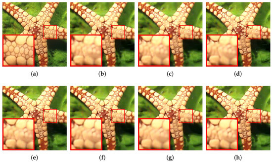
Figure 3. Denoising visual results for Starfish with $\sigma =50$. (a) Original image; (b) BM3D [29] (PSNR = 25.04 dB, SSIM = 0.7433); (c) NCSR [13] (PSNR = 25.09 dB, SSIM = 0.7453); (d) PGPD [28] (PSNR = 25.11 dB, SSIM = 0.7454); (e) GSRC-ENSS [1] (PSNR = 25.44 dB, SSIM=0.7606); (f) RRC [41] (PSNR = 25.34 dB, SSIM = 0.7589); (g) SNSS [24] (PSNR = 25.25 dB, SSIM = 0.7491); (h) HNSS-SSR (PSNR = 25.53 dB, SSIM = 0.7671).

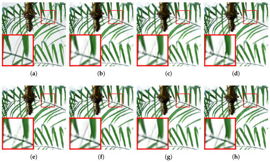
Figure 4. Denoising visual results for Leaves with $\sigma =75$. (a) Original image; (b) BM3D [29] (PSNR = 22.49 dB, SSIM = 0.8072); (c) NCSR [13] (PSNR = 22.60 dB, SSIM=0.8233); (d) PGPD [28] (PSNR = 22.61 dB, SSIM = 0.8121); (e) GSRC-ENSS [1] (PSNR = 22.90 dB, SSIM = 0.8339); (f) RRC [41] (PSNR = 22.91 dB, SSIM = 0.8377); (g) SNSS [24] (PSNR = 22.98 dB, SSIM = 0.8365); (h) HNSS-SSR (PSNR = 23.17 dB, SSIM = 0.8465).

We also evaluate the proposed HNSS-SSR on the BSD68 dataset [57]. In addition to the above methods, two recently proposed methods with excellent denoising performance, i.e., GSMM [46] and LRENSS [7], are also used to compare with our method. Table 3 lists the corresponding PSNR and SSIM results. Note that the denoising results of GSMM are quoted from Reference [46]. From Table 3, it can be seen that the proposed HNSS-SSR consistently outperforms all other methods except LRENSS. Furthermore, the denoising results of the proposed HNSS-SSR are comparable to LRENSS in terms of PSNR and SSIM.

Table 3. Average denoising result comparison of BM3D [29], NCSR [13], PGPD [28], GSRC-ENSS [1], RRC [41], SNSS [24], GSMM [46], LRENSS [7], and HNSS-SSR on the BSD68 dataset [57].

Methods	BM3D		NCSR		PGPD		GSRC-ENSS		RRC		SNSS		GSMM		LRENSS		HNSS-SSR
$\sigma =15$	31.08	0.8722	31.19	0.8770	31.13	0.8696	31.06	0.8670	31.06	0.8644	31.29	0.8765	31.32	0.8804	31.36	0.8819	31.37	0.8829
$\sigma =25$	28.56	0.8016	28.62	0.8045	28.62	0.7994	28.55	0.7985	28.56	0.7936	28.72	0.8007	28.80	0.8108	28.87	0.8122	28.85	0.8108
$\sigma =50$	25.62	0.6866	25.59	0.6864	25.75	0.6870	25.61	0.6815	25.67	0.6840	25.73	0.6876	25.85	0.6959	25.90	0.7018	25.87	0.7012
Average	28.42	0.7868	28.37	0.7893	28.50	0.7853	28.41	0.7823	28.43	0.7806	28.58	0.7883	28.66	0.7957	28.71	0.7986	28.70	0.8013

The validity of our proposed HNSS-SSR is further demonstrated by comparing it with the deep learning-based denoising approaches. Specifically, we evaluate our proposed HNSS-SSR, TNRD [19], and S2S [58] on the Set12 dataset [20]. The average PSNR and SSIM results are listed in Table 4, with the best results highlighted in bold. It can be seen that the proposed HNSS-SSR is better than TNRD and S2S across the board. In particular, the proposed HNSS-SSR achieves {0.19 dB, 0.43 dB} average PSNR gains, and {0.0072, 0.0196} average SSIM gains over TNRD and S2S, respectively.

Table 4. Average denoising result comparison of TNRD [19], S2S [58], and HNSS-SSR on the Set12 dataset [20].

Methods	$\mathit{\sigma }=15$		$\mathit{\sigma }=25$		$\mathit{\sigma }=50$		Average
TNRD	32.51	0.8967	30.06	0.8520	26.81	0.7666	29.78	0.8384
S2S	32.09	0.8894	30.04	0.8493	26.50	0.7392	29.54	0.8260
HNSS-SSR	32.64	0.8999	30.24	0.8566	27.02	0.7803	29.97	0.8456

4.2. Image Deblurring

In this subsection, we apply the proposed HNSS-SSR to image deblurring. Following prior works [13,24], we adopt the uniform blur kernel with size $9\times 9$ and the Gaussian kernel with standard deviation 1.6 to assess all deblurring approaches. For each test image, it is first blurred by a blur kernel and then corrupted by the additive white Gaussian noise with standard deviation $\sqrt{2}$ to generate the degraded image. In deblurring experiments, we set $(\sqrt{m}\times \sqrt{m},n,T,\eta ,\gamma )$ to $(6\times 6,30,200,0.04,1)$, respectively.

The deblurring performance of our proposed HNSS-SSR is verified by comparing it with several leading methods, including BM3D [59], EPLL [14], NCSR [13], JSM [60], MS-EPLL [6], and SNSS [24]. Note that BM3D, EPLL, and NCSR are three typical deblurring approaches, and JSM, MS-EPLL, and SNSS are recently developed algorithms with advanced performance. The single NSS prior is utilized by all comparison methods except SNSS, which uses both internal and external NSS priors. The deblurring results of different algorithms are presented in Table 5 and Table 6. We can observe that our proposed HNSS-SSR has the highest PSNR and SSIM in most cases compared to other competing deblurring approaches, and only SNSS is slightly better than the proposed HNSS-SSR in individual cases. Furthermore, for uniform blur, the proposed HNSS-SSR achieves {1.35 dB, 3.25 dB, 0.33 dB, 3.16 dB, 2.85 dB, 0.18 dB} average PSNR gains and {0.0391, 0.0391, 0.0135, 0.1672, 0.0340, 0.0030} average SSIM gains over BM3D, EPLL, NCSR, JSM, MS-EPLL, and SNSS, respectively. For Gaussian blur, our proposed HNSS-SSR achieves {1.22 dB, 5.51 dB, 0.67 dB, 1.64 dB, 4.78 dB, 0.35 dB} average PSNR gains and {0.0265, 0.0440, 0.0214, 0.0675, 0.0408, 0.0034} average SSIM gains over BM3D, EPLL, NCSR, JSM, MS-EPLL, and SNSS, respectively. The visual deblurring results of different approaches are presented in Figure 5 and Figure 6. It can be obviously observed that BM3D, NCSR, JSM, and MS-EPLL produce a lot of unpleasant artifacts, while EPLL and SNSS cause over-smoothing phenomena. In comparison, our proposed HNSS-SSR method effectively eliminates artifacts while delivering a friendly visual perception.

Table 5. PSNR comparison of BM3D [59], EPLL [14], NCSR [13], JSM [60], MS-EPLL [6], SNSS [24], and HNSS-SSR for image deblurring.

	Uniform Blur, $\mathit{\sigma }=\sqrt{2}$							Gaussian Blur, $\mathit{\sigma }=\sqrt{2}$
Methods	BM3D	EPLL	NCSR	JSM	MS- EPLL	SNSS	HNSS- SSR	BM3D	EPLL	NCSR	JSM	MS- EPLL	SNSS	HNSS- SSR
Bear	30.49	28.87	31.14	28.09	29.15	31.37	31.48	31.99	27.63	32.25	31.30	29.99	32.66	32.82
Bike	24.57	23.19	25.41	23.89	23.92	25.47	25.26	26.65	22.92	26.98	26.65	23.49	26.90	27.22
Buddhist	34.33	33.44	35.02	29.93	33.29	35.35	35.59	36.91	34.46	36.90	34.42	33.55	38.24	38.35
Butterfly	26.80	24.44	28.83	25.65	25.26	29.14	29.52	28.58	22.00	29.78	28.79	22.75	30.20	31.00
Cameraman	27.30	26.02	28.59	26.20	26.82	28.67	28.67	27.46	26.62	28.31	27.45	27.43	28.13	28.24
Corn	26.75	24.56	27.87	25.55	25.26	28.24	28.58	28.91	23.89	29.69	29.00	24.42	30.08	30.45
Cowboy	27.19	25.93	27.99	25.90	26.54	28.09	28.02	28.05	24.86	28.45	27.95	26.59	28.47	28.65
Flower	28.58	27.04	29.38	26.88	27.61	29.37	29.55	30.41	26.64	30.82	30.01	27.34	31.08	31.42
Flowers	28.54	26.31	29.28	26.87	26.74	29.31	29.42	29.84	25.14	30.20	29.51	27.20	30.25	30.52
Girls	26.47	24.00	27.15	25.29	24.00	27.22	27.34	27.82	22.70	28.11	27.72	23.21	28.15	28.50
Hat	30.63	29.22	31.30	28.23	29.44	31.45	31.60	31.78	29.20	32.24	31.06	28.04	32.53	32.76
Lake	27.32	25.12	28.12	25.90	25.74	28.06	28.41	29.17	22.60	29.48	28.91	26.23	29.63	29.91
Leaves	26.89	23.46	28.98	25.48	23.48	29.08	29.60	29.00	21.38	30.34	29.16	21.53	30.69	31.63
Lena	30.35	28.13	31.26	28.00	28.46	31.32	31.53	32.24	28.00	32.67	31.46	26.64	33.02	33.33
Plants	32.07	29.83	33.12	28.88	29.58	33.52	33.78	33.99	30.18	34.65	32.87	31.35	35.59	35.93
Starfish	28.08	26.32	29.20	26.63	27.08	29.42	29.63	30.20	26.20	30.98	30.08	26.35	31.40	31.76
Average	28.52	26.62	29.54	26.71	27.02	29.69	29.87	30.19	25.90	30.74	29.77	26.63	31.06	31.41

Table 6. SSIM comparison of BM3D [59], EPLL [14], NCSR [13], JSM [60], MS-EPLL [6], SNSS [24], and HNSS-SSR for image deblurring.

	Uniform Blur, $\mathit{\sigma }=\sqrt{2}$							Gaussian Blur, $\mathit{\sigma }=\sqrt{2}$
Methods	BM3D	EPLL	NCSR	JSM	MS- EPLL	SNSS	HNSS- SSR	BM3D	EPLL	NCSR	JSM	MS- EPLL	SNSS	HNSS- SSR
Bear	0.8074	0.8251	0.8269	0.6621	0.8263	0.8386	0.8405	0.8618	0.8560	0.8618	0.8134	0.8673	0.8836	0.8852
Bike	0.7589	0.7393	0.7996	0.7046	0.7741	0.8081	0.8019	0.8511	0.8082	0.8599	0.8403	0.8274	0.8678	0.8730
Buddhist	0.8979	0.9158	0.9026	0.6701	0.8926	0.9205	0.9246	0.9337	0.9434	0.9256	0.8481	0.9297	0.9583	0.9563
Butterfly	0.8714	0.8743	0.9076	0.7629	0.8852	0.9212	0.9251	0.9157	0.8840	0.9220	0.8814	0.8922	0.9422	0.9470
Cameraman	0.8258	0.8345	0.8568	0.6731	0.8256	0.8592	0.8631	0.8416	0.8486	0.8547	0.7845	0.8271	0.8732	0.8756
Corn	0.8406	0.8175	0.8692	0.7753	0.8324	0.8844	0.8909	0.8970	0.8619	0.9079	0.8860	0.8678	0.9221	0.9264
Cowboy	0.8452	0.8544	0.8668	0.7181	0.8580	0.8766	0.8776	0.8861	0.8698	0.8880	0.8452	0.8838	0.9031	0.9045
Flower	0.8119	0.7984	0.8392	0.6937	0.8173	0.8445	0.8484	0.8701	0.8511	0.8773	0.8340	0.8608	0.8925	0.8975
Flowers	0.8022	0.7980	0.8273	0.6553	0.8105	0.8402	0.8402	0.8592	0.8397	0.8617	0.8081	0.8569	0.8773	0.8827
Girls	0.7907	0.7853	0.8216	0.7240	0.8081	0.8307	0.8310	0.8537	0.8203	0.8626	0.8404	0.8353	0.8732	0.8780
Hat	0.8427	0.8435	0.8505	0.6428	0.8220	0.8597	0.8645	0.8637	0.8673	0.8674	0.7938	0.8384	0.8909	0.8930
Lake	0.8230	0.8285	0.8471	0.7021	0.8288	0.8538	0.8609	0.8836	0.8566	0.8865	0.8457	0.8633	0.9021	0.9061
Leaves	0.8947	0.8792	0.9345	0.8179	0.8950	0.9410	0.9470	0.9338	0.8922	0.9452	0.9153	0.8986	0.9587	0.9654
Lena	0.8563	0.8649	0.8753	0.6966	0.8606	0.8862	0.8903	0.9028	0.8976	0.9036	0.8485	0.8944	0.9246	0.9267
Plants	0.8563	0.8636	0.8745	0.6707	0.8579	0.8932	0.8969	0.9042	0.9000	0.9057	0.8405	0.9011	0.9336	0.9349
Starfish	0.8178	0.8205	0.8521	0.7238	0.8290	0.8621	0.8652	0.8849	0.8653	0.8937	0.8612	0.8696	0.9094	0.9136
Average	0.8339	0.8339	0.8595	0.7058	0.8390	0.8700	0.8730	0.8839	0.8664	0.8890	0.8429	0.8696	0.9070	0.9104

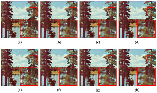
Figure 5. Deblurring results for Lake with uniform kernel. (a) Original image; (b) BM3D [59] (PSNR = 27.32 dB, SSIM = 0.8230); (c) EPLL [14] (PSNR = 25.12 dB, SSIM = 0.8285); (d) NCSR [13] (PSNR = 28.12 dB, SSIM = 0.8471); (e) JSM [60] (PSNR = 25.90 dB, SSIM = 0.7021); (f) MS-EPLL [6] (PSNR = 25.74 dB, SSIM = 0.8288); (g) SNSS [24] (PSNR = 28.06 dB, SSIM = 0.8538); (h) HNSS-SSR (PSNR = 28.41 dB, SSIM = 0.8609).

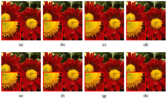
Figure 6. Deblurring results for Flowers with Gaussian kernel. (a) Original image; (b) BM3D [59] (PSNR = 29.84 dB, SSIM = 0.8592); (c) EPLL [14] (PSNR = 25.14 dB, SSIM = 0.8397); (d) NCSR [13] (PSNR = 30.20 dB, SSIM = 0.8617); (e) JSM [60] (PSNR = 29.51 dB, SSIM = 0.8081); (f) MS-EPLL [6] (PSNR = 27.20 dB, SSIM = 0.8569); (g) SNSS [24] (PSNR = 30.25 dB, SSIM = 0.8773); (h) HNSS-SSR (PSNR = 30.52 dB, SSIM = 0.8827).

The proposed HNSS-SSR is also tested on the Set14 dataset [61], and compared with the recently proposed JGD-SSR model [3] and LRENSS prior [7]. Note that JGD-SSR jointly utilizes the internal and external NSS priors, while LRENSS jointly utilizes the low-rank prior and external NSS prior. The average PSNR and SSIM results are listed in Table 7. It can be seen that the proposed HNSS-SSR has performance comparable to JGD-SSR and LRENSS and has considerable PSNR and SSIM gains compared to other methods.

Table 7. Average deblurring result comparison of BM3D [59], EPLL [14], NCSR [13], JSM [60], MS-EPLL [6], SNSS [24], JGD-SSR [3], LRENSS [7], and HNSS-SSR on the Set14 dataset [61].

Methods	BM3D		EPLL		NCSR		JSM		MS-EPLL		SNSS		JGD-SSR		LRENSS		HNSS-SSR
Uniform	29.13	0.8026	27.23	0.7979	30.03	0.8239	27.22	0.6819	27.26	0.8050	30.00	0.8222	30.38	0.8294	30.25	0.8308	30.34	0.8289
Gaussian	30.20	0.8544	27.21	0.8371	30.74	0.8529	29.86	0.8080	28.69	0.8434	30.96	0.8631	31.35	0.8683	31.30	0.8703	31.38	0.8697
Average	29.67	0.8285	27.22	0.8175	30.39	0.8384	28.54	0.7450	28.19	0.8242	30.48	0.8427	30.87	0.8489	30.78	0.8506	30.86	0.8493

The benefit of our proposed HNSS-SSR is further evidenced by making a comparison with deep learning-based approaches, specifically involving RED [62], IRCNN [63], and H-PnP [64], on the Set14 dataset [61]. Table 8 presents the deblurring results. One can clearly see that our proposed HNSS-SSR is far preferable to RED. Meanwhile, the proposed HNSS-SSR not only yields comparable PSNR results with IRCNN and H-PnP, but also has the best SSIM results. As we all know, SSIM is more consistent with human vision than PSNR, so SSIM can usually lead to a more objective quantitative evaluation [56]. In particular, the SSIM gains of our proposed HNSS-SSR over RED, IRCNN, and H-PnP are 0.0081, 0.0045, and 0.0038, respectively.

Table 8. Average deblurring result comparison of RED [62], IRCNN [63], H-PnP [64], and HNSS-SSR on the Set14 dataset [61].

Methods	Uniform Blur		Gaussian Blur		Average
RED	30.03	0.8238	30.91	0.8566	30.47	0.8402
IRCNN	30.30	0.8281	31.29	0.8596	30.78	0.8438
H-PnP	30.25	0.8238	31.33	0.8651	30.79	0.8445
HNSS-SSR	30.34	0.8289	31.38	0.8697	30.86	0.8493

4.3. Computational Time

In this subsection, we report the running time of different denoising and deblurring methods on the $256\times 256$ image in Table 9. All methods are tested on Intel® Core™ i7-9700 3.00 GHz CPU PC under the MATLAB 2019a environment. Note that the experimental results of GSMM are obtained from Reference [46], so its running time is not reported here. One can see that, for image denoising, the proposed HNSS-SSR is slower than only BM3D and PGPD, and for image deblurring, the proposed HNSS-SSR is faster than SNSS and LRENSS.

Table 9. Running time in seconds (s) of different denoising and deblurring methods.

Image Denoising ($\mathit{\sigma }=50$)
Methods	BM3D [29]	NCSR [13]	PGPD [28]	GSRC-ENSS [1]	RRC [41]	SNSS [24]	GSMM [46]	LRENSS [7]	HNSS-SSR
Time (s)	0.8	224.3	8.3	369.2	226.6	602.1	-	108.6	49.4
Image Deblurring
Methods	BM3D [59]	EPLL [14]	NCSR [13]	JSM [60]	MS-EPLL [6]	SNSS [24]	JGD-SSR [3]	LRENSS [7]	HNSS-SSR
Time (s)	0.9	49.7	98.1	158.9	214.2	4830.4	405.8	707.6	690.3

5. Conclusions

This paper proposed to learn a new NSS prior, namely the HNSS prior, from both internal and external image data and applied it to the image restoration problem. Two sets of GMMs for depicting internal and external NSS priors were first learned from the degraded observation and natural image sets, respectively. Subsequently, based on learned internal and external priors, the HNSS prior that can better characterize the image structure and detail information was efficiently learned by SVD and a simple weighting method. An HNSS prior-based structural sparse representation (HNSS-SSR) model with adaptive regularization parameters was then formulated for the image restoration problem. Further, we adopted an alternate minimization strategy to solve the corresponding restoration problem, resulting in a general restoration algorithm. Experimental results have validated that, compared to many classical or excellent approaches, our proposed HNSS-SSR algorithm not only provides better visual results but also yields competitive PSNR and SSIM metrics.

References

- Zha, Z.; Zhang, X.; Wang, Q.; Bai, Y.; Chen, Y.; Tang, L.; Liu, X. Group sparsity residual constraint for image denoising with external nonlocal self-similarity prior. Neurocomputing 2018, 275, 2294–2306. [Google Scholar] [CrossRef]
- Yuan, W.; Liu, H.; Liang, L.; Xie, G.; Zhang, Y.; Liu, D. Rank minimization via adaptive hybrid norm for image restoration. Signal Process. 2023, 206, 108926. [Google Scholar] [CrossRef]
- Yuan, W.; Liu, H.; Liang, L. Joint group dictionary-based structural sparse representation for image restoration. Digit. Signal Process. 2023, 137, 104029. [Google Scholar] [CrossRef]
- Zhang, J.; Zhao, D.; Gao, W. Group-based sparse representation for image restoration. IEEE Trans. Image Process. 2014, 23, 3336–3351. [Google Scholar] [CrossRef] [PubMed]
- Zha, Z.; Wen, B.; Yuan, X.; Zhou, J.; Zhu, C.; Kot, A.C. A hybrid structural sparsification error model for image restoration. IEEE Trans. Neural Networks Learn. Syst. 2021, 33, 4451–4465. [Google Scholar] [CrossRef] [PubMed]
- Papyan, V.; Elad, M. Multi-scale patch-based image restoration. IEEE Trans. Image Process. 2016, 25, 249–261. [Google Scholar] [CrossRef] [PubMed]
- Yuan, W.; Liu, H.; Liang, L.; Wang, W.; Liu, D. Image restoration via joint low-rank and external nonlocal self-similarity prior. Signal Process. 2024, 215, 109284. [Google Scholar] [CrossRef]
- Aharon, M.; Elad, M.; Bruckstein, A. K-SVD: An algorithm for designing overcomplete dictionaries for sparse representation. IEEE Trans. Signal Process. 2006, 54, 4311–4322. [Google Scholar] [CrossRef]
- Elad, M.; Aharon, M. Image denoising via sparse and redundant representations over learned dictionaries. IEEE Trans. Image Process. 2006, 15, 3736–3745. [Google Scholar] [CrossRef]
- Mairal, J.; Elad, M.; Sapiro, G. Sparse representation for color image restoration. IEEE Trans. Image Process. 2007, 17, 53–69. [Google Scholar] [CrossRef]
- Dong, W.; Zhang, L.; Shi, G.; Wu, X. Image deblurring and super-resolution by adaptive sparse domain selection and adaptive regularization. IEEE Trans. Image Process. 2011, 20, 1838–1857. [Google Scholar] [CrossRef] [PubMed]
- Gai, S. Theory of reduced biquaternion sparse representation and its applications. Expert Syst. Appl. 2023, 213, 119245. [Google Scholar] [CrossRef]
- Dong, W.; Zhang, L.; Shi, G.; Li, X. Nonlocally centralized sparse representation for image restoration. IEEE Trans. Image Process. 2013, 22, 1620–1630. [Google Scholar] [CrossRef] [PubMed]
- Zoran, D.; Weiss, Y. From learning models of natural image patches to whole image restoration. In Proceedings of the IEEE International Conference on Computer Vision, Barcelona, Spain, 6–13 November 2011; pp. 479–486. [Google Scholar]
- Yu, G.; Sapiro, G.; Mallat, S. Solving inverse problems with piecewise linear estimators: From Gaussian mixture models to structured sparsity. IEEE Trans. Image Process. 2012, 21, 2481–2499. [Google Scholar] [PubMed]
- Colak, O.; Eksioglu, E.M. On the fly image denoising using patch ordering. Expert Syst. Appl. 2022, 190, 116192. [Google Scholar] [CrossRef]
- Burger, H.C.; Schuler, C.J.; Harmeling, S. Image denoising: Can plain neural networks compete with BM3D? In Proceedings of the IEEE Conference on Computer Vision and Pattern Recognition, Providence, RI, USA, 16–21 June 2012; pp. 2392–2399. [Google Scholar]
- Wang, J.; Wang, Z.; Yang, A. Iterative dual CNNs for image deblurring. Mathematics 2022, 10, 3891. [Google Scholar] [CrossRef]
- Chen, Y.; Pock, T. Trainable nonlinear reaction diffusion: A flexible framework for fast and effective image restoration. IEEE Trans. Pattern Anal. Mach. Intell. 2017, 39, 1256–1272. [Google Scholar] [CrossRef] [PubMed]
- Zhang, K.; Zuo, W.; Chen, Y.; Meng, D.; Zhang, L. Beyond a gaussian denoiser: Residual learning of deep cnn for image denoising. IEEE Trans. Image Process. 2017, 26, 3142–3155. [Google Scholar] [CrossRef]
- Zhang, K.; Li, Y.; Zuo, W.; Zhang, L.; Van Gool, L.; Timofte, R. Plug-and-play image restoration with deep denoiser prior. IEEE Trans. Pattern Anal. Mach. Intell. 2021, 44, 6360–6376. [Google Scholar] [CrossRef]
- Li, X.; Wang, J.; Liu, X. Deep Successive Convex Approximation for Image Super-Resolution. Mathematics 2023, 11, 651. [Google Scholar] [CrossRef]
- Yuan, W.; Liu, H.; Liang, L. Image restoration via exponential scale mixture-based simultaneous sparse prior. IET Image Process. 2022, 16, 3268–3283. [Google Scholar] [CrossRef]
- Zha, Z.; Yuan, X.; Zhou, J.; Zhu, C.; Wen, B. Image restoration via simultaneous nonlocal self-similarity priors. IEEE Trans. Image Process. 2020, 29, 8561–8576. [Google Scholar] [CrossRef] [PubMed]
- Zha, Z.; Yuan, X.; Wen, B.; Zhang, J.; Zhou, J.; Zhu, C. Simultaneous nonlocal self-similarity prior for image denoising. In Proceedings of the IEEE International Conference on Image Processing, Taipei, Taiwan, 22–25 September 2019; pp. 1119–1123. [Google Scholar]
- Wen, B.; Li, Y.; Bresler, Y. Image recovery via transform learning and low-rank modeling: The power of complementary regularizers. IEEE Trans. Image Process. 2020, 29, 5310–5323. [Google Scholar] [CrossRef] [PubMed]
- Buades, A.; Coll, B.; Morel, J.M. A non-local algorithm for image denoising. In Proceedings of the IEEE Conference on Computer Vision and Pattern Recognition, San Diego, CA, USA, 20–26 June 2005; Volume 2, pp. 60–65. [Google Scholar]
- Xu, J.; Zhang, L.; Zuo, W.; Zhang, D.; Feng, X. Patch group based nonlocal self-similarity prior learning for image denoising. In Proceedings of the IEEE International Conference on Computer Vision, Santiago, Chile, 7–13 December 2015; pp. 244–252. [Google Scholar]
- Dabov, K.; Foi, A.; Katkovnik, V.; Egiazarian, K. Image denoising by sparse 3-D transform-domain collaborative filtering. IEEE Trans. Image Process. 2007, 16, 2080–2095. [Google Scholar] [CrossRef] [PubMed]
- Hou, Y.; Xu, J.; Liu, M.; Liu, G.; Liu, L.; Zhu, F.; Shao, L. NLH: A blind pixel-level non-local method for real-world image denoising. IEEE Trans. Image Process. 2020, 29, 5121–5135. [Google Scholar] [CrossRef]
- Mairal, J.; Bach, F.; Ponce, J.; Sapiro, G.; Zisserman, A. Non-local sparse models for image restoration. In Proceedings of the IEEE International Conference on Computer Vision, Kyoto, Japan, 29 September–2 October 2009; pp. 2272–2279. [Google Scholar]
- Dong, W.; Shi, G.; Ma, Y.; Li, X. Image restoration via simultaneous sparse coding: Where structured sparsity meets gaussian scale mixture. Int. J. Comput. Vis. 2015, 114, 217–232. [Google Scholar] [CrossRef]
- Yuan, W.; Liu, H.; Liang, L.; Wang, W.; Liu, D. A hybrid structural sparse model for image restoration. Opt. Laser Technol. 2022, 171, 110401. [Google Scholar] [CrossRef]
- Ou, Y.; Swamy, M.; Luo, J.; Li, B. Single image denoising via multi-scale weighted group sparse coding. Signal Process. 2022, 200, 108650. [Google Scholar] [CrossRef]
- Zha, Z.; Yuan, X.; Wen, B.; Zhou, J.; Zhu, C. Group sparsity residual constraint with non-local priors for image restoration. IEEE Trans. Image Process. 2020, 29, 8960–8975. [Google Scholar] [CrossRef]
- Zha, Z.; Yuan, X.; Wen, B.; Zhang, J.; Zhou, J.; Zhu, C. Image restoration using joint patch-group-based sparse representation. IEEE Trans. Image Process. 2020, 29, 7735–7750. [Google Scholar] [CrossRef]
- Zha, Z.; Wen, B.; Yuan, X.; Zhou, J.; Zhu, C. Image restoration via reconciliation of group sparsity and low-rank models. IEEE Trans. Image Process. 2021, 30, 5223–5238. [Google Scholar] [CrossRef] [PubMed]
- Zha, Z.; Wen, B.; Yuan, X.; Zhou, J.; Zhu, C.; Kot, A.C. Low-rankness guided group sparse representation for image restoration. IEEE Trans. Neural Netw. Learn. Syst. 2022, 34, 7593–7607. [Google Scholar] [CrossRef]
- Dong, W.; Shi, G.; Li, X. Nonlocal image restoration with bilateral variance estimation: A low-rank approach. IEEE Trans. Image Process. 2012, 22, 700–711. [Google Scholar] [CrossRef]
- Gu, S.; Xie, Q.; Meng, D.; Zuo, W.; Feng, X.; Zhang, L. Weighted nuclear norm minimization and its applications to low level vision. Int. J. Comput. Vis. 2017, 121, 183–208. [Google Scholar] [CrossRef]
- Zha, Z.; Yuan, X.; Wen, B.; Zhou, J.; Zhang, J.; Zhu, C. From rank estimation to rank approximation: Rank residual constraint for image restoration. IEEE Trans. Image Process. 2019, 29, 3254–3269. [Google Scholar] [CrossRef] [PubMed]
- Chen, J.F.; Wang, Q.W.; Song, G.J.; Li, T. Quaternion matrix factorization for low-rank quaternion matrix completion. Mathematics 2023, 11, 2144. [Google Scholar] [CrossRef]
- Xu, C.; Liu, X.; Zheng, J.; Shen, L.; Jiang, Q.; Lu, J. Nonlocal low-rank regularized two-phase approach for mixed noise removal. Inverse Probl. 2021, 37, 085001. [Google Scholar] [CrossRef]
- Lu, J.; Xu, C.; Hu, Z.; Liu, X.; Jiang, Q.; Meng, D.; Lin, Z. A new nonlocal low-rank regularization method with applications to magnetic resonance image denoising. Inverse Probl. 2022, 38, 065012. [Google Scholar] [CrossRef]
- Li, H.; Jia, X.; Zhang, L. Clustering based content and color adaptive tone mapping. Comput. Vis. Image Underst. 2018, 168, 37–49. [Google Scholar] [CrossRef]
- Liu, H.; Li, L.; Lu, J.; Tan, S. Group sparsity mixture model and its application on image denoising. IEEE Trans. Image Process. 2022, 31, 5677–5690. [Google Scholar] [CrossRef]
- Xu, J.; Zhang, L.; Zhang, D. External prior guided internal prior learning for real-world noisy image denoising. IEEE Trans. Image Process. 2018, 27, 2996–3010. [Google Scholar] [CrossRef] [PubMed]
- Yue, H.; Sun, X.; Yang, J.; Wu, F. CID: Combined image denoising in spatial and frequency domains using Web images. In Proceedings of the IEEE Conference on Computer Vision and Pattern Recognition, Mandi, India, 16–19 December 2014; pp. 2933–2940. [Google Scholar]
- Liu, J.; Yang, W.; Zhang, X.; Guo, Z. Retrieval compensated group structured sparsity for image super-resolution. IEEE Trans. Multimed. 2017, 19, 302–316. [Google Scholar] [CrossRef]
- Zoran, D.; Weiss, Y. Natural images, Gaussian mixtures and dead leaves. In Advances in Neural Information Processing Systems; MIT Press: Cambridge, MA, USA, 2012; Volume 25. [Google Scholar]
- Keller, J.M.; Gray, M.R.; Givens, J.A. A fuzzy k-nearest neighbor algorithm. IEEE Trans. Syst. Man Cybern. 1985, SMC-15, 580–585. [Google Scholar]
- Niknejad, M.; Rabbani, H.; Babaie-Zadeh, M. Image restoration using Gaussian mixture models with spatially constrained patch clustering. IEEE Trans. Image Process. 2015, 24, 3624–3636. [Google Scholar] [CrossRef]
- Wu, C.J. On the convergence properties of the EM algorithm. Ann. Stat. 1983, 11, 95–103. [Google Scholar] [CrossRef]
- Daubechies, I.; Defrise, M.; De Mol, C. An iterative thresholding algorithm for linear inverse problems with a sparsity constraint. Commun. Pure Appl. Math. A J. Issued Courant Inst. Math. Sci. 2004, 57, 1413–1457. [Google Scholar] [CrossRef]
- Osher, S.; Burger, M.; Goldfarb, D.; Xu, J.; Yin, W. An iterative regularization method for total variation-based image restoration. Multiscale Model. Simul. 2005, 4, 460–489. [Google Scholar] [CrossRef]
- Wang, Z.; Bovik, A.C.; Sheikh, H.R.; Simoncelli, E.P. Image quality assessment: From error visibility to structural similarity. IEEE Trans. Image Process. 2004, 13, 600–612. [Google Scholar] [CrossRef] [PubMed]
- Arbelaez, P.; Maire, M.; Fowlkes, C.; Malik, J. Contour detection and hierarchical image segmentation. IEEE Trans. Pattern Anal. Mach. Intell. 2010, 33, 898–916. [Google Scholar] [CrossRef] [PubMed]
- Quan, Y.; Chen, M.; Pang, T.; Ji, H. Self2self with dropout: Learning self-supervised denoising from single image. In Proceedings of the IEEE Conference on Computer Vision and Pattern Recognition, Seattle, WA, USA, 14–19 June 2020; pp. 1890–1898. [Google Scholar]
- Dabov, K.; Foi, A.; Katkovnik, V.; Egiazarian, K. Image restoration by sparse 3D transform-domain collaborative filtering. In Proceedings of the Image Processing: Algorithms and Systems VI, San Jose, CA, USA, 28–29 January 2008; pp. 62–73. [Google Scholar]
- Zhang, J.; Zhao, D.; Xiong, R.; Ma, S.; Gao, W. Image restoration using joint statistical modeling in a space-transform domain. IEEE Trans. Circuits Syst. Video Technol. 2014, 24, 915–928. [Google Scholar] [CrossRef]
- Zeyde, R.; Elad, M.; Protter, M. On single image scale-up using sparse-representations. In Proceedings of the Curves and Surfaces: 7th International Conference, Avignon, France, 24–30 June 2010; pp. 711–730. [Google Scholar]
- Romano, Y.; Elad, M.; Milanfar, P. The little engine that could: Regularization by denoising (RED). SIAM J. Imaging Sci. 2017, 10, 1804–1844. [Google Scholar] [CrossRef]
- Zhang, K.; Zuo, W.; Gu, S.; Zhang, L. Learning deep CNN denoiser prior for image restoration. In Proceedings of the IEEE Conference on Computer Vision and Pattern Recognition, Honolulu, HI, USA, 21–26 July 2017; pp. 3929–3938. [Google Scholar]
- Zha, Z.; Wen, B.; Yuan, X.; Zhou, J.T.; Zhou, J.; Zhu, C. Triply complementary priors for image restoration. IEEE Trans. Image Process. 2021, 30, 5819–5834. [Google Scholar] [CrossRef] [PubMed]
Disclaimer/Publisher’s Note: The statements, opinions and data contained in all publications are solely those of the individual author(s) and contributor(s) and not of MDPI and/or the editor(s). MDPI and/or the editor(s) disclaim responsibility for any injury to people or property resulting from any ideas, methods, instructions or products referred to in the content. |
© 2024 by the authors. Licensee MDPI, Basel, Switzerland. This article is an open access article distributed under the terms and conditions of the Creative Commons Attribution (CC BY) license (https://creativecommons.org/licenses/by/4.0/).