FEBE-Net: Feature Exploration Attention and Boundary Enhancement Refinement Transformer Network for Bladder Tumor Segmentation

Abstract

The automatic and accurate segmentation of bladder tumors is a key step in assisting urologists in diagnosis and analysis. At present, existing Transformer-based methods have limited ability to restore local detail features and insufficient boundary segmentation capabilities. We propose FEBE-Net, which aims to effectively capture global and remote semantic features, preserve more local detail information, and provide clearer and more precise boundaries. Specifically, first, we use PVT v2 backbone to learn multi-scale global feature representations to adapt to changes in bladder tumor size and shape. Secondly, we propose a new feature exploration attention module (FEA) to fully explore the potential local detail information in the shallow features extracted by the PVT v2 backbone, eliminate noise, and supplement the missing fine-grained details for subsequent decoding stages. At the same time, we propose a new boundary enhancement and refinement module (BER), which generates high-quality boundary clues through boundary detection operators to help the decoder more effectively preserve the boundary features of bladder tumors and refine and adjust the final predicted feature map. Then, we propose a new efficient self-attention calibration decoder module (ESCD), which, with the help of boundary clues provided by the BER module, gradually and effectively recovers global contextual information and local detail information from high-level features after calibration enhancement and low-level features after exploration attention. Extensive experiments on the cystoscopy dataset BtAMU and five colonoscopy datasets have shown that FEBE-Net outperforms 11 state-of-the-art (SOTA) networks in segmentation performance, with higher accuracy, stronger robust stability, and generalization ability.

1. Introduction

Bladder cancer ranks among the ten most common cancers worldwide [1]. However, through surgical treatment, the cure rate of early bladder cancer is very high [2]. Therefore, the early detection and resection of bladder tumors is crucial to improve the cure rate of bladder cancer. At present, cystoscopy is one of the main screening methods for early bladder tumors. In clinical practice, it is of great significance to develop an automatic, accurate, and robust segmentation algorithm for bladder tumors based on cystoscopy images to reduce the dependence on visual examination by urologists and improve the accuracy of bladder tumor detection. However, due to the diversity in the morphology and size of bladder tumors, the presence of folds in the bladder wall, and the relatively low brightness of cystoscopy images, the segmentation task for bladder tumors still poses challenges.

In recent years, CNNs (Convolutional Neural Networks) have demonstrated strong performance in tasks related to medical image segmentation [3,4], such as breast ultrasound image segmentation [5], skin lesion segmentation [6], multi-organ CT image segmentation, polyp segmentation [7,8], and liver lesion segmentation. Although CNN-based medical image segmentation methods [3,4,5,6,7,8,9,10,11,12,13,14,15,16,17,18,19] have achieved initial success, due to the locality of convolution operations and limited kernel size, the CNN has a weak ability to learn global contextual information, which is crucial for accurately segmenting lesions or organ tissues with significant differences in shape and size. To overcome this limitation, some studies [20,21] have attempted to use non-local self-attention mechanisms based on CNN features to simulate global scenes. However, they are only applicable to low-resolution medical images, and the computational complexity of these modules is too high in high-resolution images. Other studies [22,23] have attempted to expand the receptive field of convolutional kernels, but this requires continuous downsampling operations and stacking sufficiently deep convolutional layers, which not only leads to the loss of small target areas, and network redundancy, but more importantly, effective receptive fields are still limited to local areas. In summary, regarding the task of bladder tumor segmentation, CNNs have limitations in capturing long-range dependencies.

Recently, the emergence of Vision Transformer (ViT) [24], which does not require any convolution operations and relies solely on self-attention mechanisms, has solved the problem of CNN’s insufficient ability to learn remote dependency relationships. Specifically, Transformers [24,25,26,27,28] calculate the similarity of all patch pairs using the dot product of patch vectors, allowing it to adaptively extract and blend features between all patches. This approach provides the Transformers with an effective global receptive field and minimizes the model’s inductive bias [29]. Therefore, compared to CNN-based methods, vision-converter-based methods [24,25,26,27,28] have a stronger ability to extract global information and a stronger generalization ability, greatly improving the accuracy of medical image analysis tasks such as recognition, segmentation, and diagnosis. Although Transformer-based methods [29,30,31,32,33,34,35,36,37,38] have achieved significant success in medical image segmentation tasks, they still face limitations in capturing fine-grained detail information of bladder tumors due to the lack of spatially induced bias in modeling local information [39]. In addition, these methods do not pay enough attention to the boundary areas of medical images (such as cystoscopy images), which may lead to unclear boundaries of the predicted target (bladder tumor) area.

To achieve the advantages of the CNN and Transformer, recent studies [39,40,41,42,43,44,45,46] have attempted to combine the CNN and Transformer, mainly divided into a serial branch structure and parallel branch structure. The encoder of the hybrid network with a serial structure [40,41] stacks CNN layers and Transformer layers sequentially. However, this serial structure only uses the context modeling self-attention mechanism at a single scale, which neglects cross-scale dependencies and consistency [6], and does not fully leverage the advantages of the Transformer. The hybrid network employs a parallel structure [39,42,43,44,45,46,47], utilizing the Transformer branch for global feature extraction and the CNN branch for local feature extraction, followed by fusing the features from both branches. However, the simple and rough fusion ignores the semantic gap between the two features, and the parallel-running dual encoder structure also significantly increases the computational complexity.

At present, most deep learning-based medical image segmentation networks focus on designing fine modules to enhance the features extracted by the CNN or Transformer backbone networks and fuse contextual information, while ignoring the importance of boundary feature information for prediction results. This may lead to inaccurate or discontinuous prediction boundaries, resulting in unsatisfactory final prediction results. To address this issue, some studies [14,48,49,50,51] have designed specialized modules to capture boundary feature information, such as the reverse attention module [14], Residual Axial Reverse Attention (RA-RA) [49], and Balancing Attention Module (BAM) [50]. However, due to the lack of boundary supervision in these methods, in some medical images, especially those with blurred boundaries, directly exploring boundary clues using foreground (target) supervision may not be accurate. Other studies attempt to predict boundary regions under boundary supervision conditions [5,52]. They add boundary prediction results to the target prediction results, which to some extent refine the final segmentation results. However, their boundary prediction tasks and target prediction tasks are independent and do not communicate with each other. These methods can only refine the final target prediction results and cannot provide boundary clues for the target prediction process.

Therefore, we propose a new network model based on Transformer for the automatic and accurate segmentation of bladder tumors, FEBE-Net, which aims to extract multi-scale global information (capturing global features across multiple image scales), enhance local feature information representation, and improve the learning ability and boundary segmentation accuracy of the model by capturing boundary features. Firstly, we choose the PVT v2 encoder [28] as the backbone network to effectively capture multi-scale global features of bladder tumors, accommodating variations in tumor shape and size. Next, we propose the new feature exploration attention module (FEA) to explore potential bladder tumor local detail feature information in the first three layers of features extracted by the encoder. The four branches of the FEA module perform different convolution operations on low-level features to capture local information. The fourth branch uses self-calibration convolution [53] to capture richer fine-grained detail features and then concatenates the features extracted by the four branches to help enhance the features. Subsequently, the LECA module [34] is used to filter background noise, purify feature information, and then supplement it with the corresponding high-level features at the decoder end through horizontal connections to bridge semantic gaps. Then, we use one $1\times 1$ convolutional unit and three new proposed efficient self-attention calibration decoding modules (ESCD) to gradually output high-resolution prediction masks. ESCD utilizes an efficient self-attention mechanism to recover global features and then filters out more valuable contextual key information through the channel attention module (CAM) [54] and convolutional attention module. The calibrated enhanced global features are then multiplied with the fine-grained detail features output by the FEA module to continuously supplement rich local detail features. At the same time, we utilize the proposed new boundary enhancement and refinement module (BER) to process the first- and fourth-layer features extracted by the encoder to generate high-quality boundary clues, integrate them into the bladder tumor prediction task, and use an adaptive weighting strategy to enhance the boundary regions in the advanced features of the decoder. We also use boundary clues to fine-tune the final prediction map to achieve complementary fusion, making the network generate more accurate positioning and clearer boundary prediction masks. Finally, we design a hybrid supervision strategy to achieve the dual supervision of bladder tumor prediction masks and boundary masks. To verify the segmentation performance of the proposed model, we conducted extensive experiments on the cystoscopy dataset BtAMU [55] and five publicly available colonoscopy datasets [56,57,58,59,60]. The effectiveness and generalization of the proposed method were superior to other state-of-the-art (SOTA) methods. Among them, on BtAMU [55], the mDice and mIoU indicators of the proposed method reached 0.9126 and 0.8578, respectively, which were 1% and 1.4% higher than that of MSGAT [38]. Specifically, on the most challenging ETIS [60] dataset, the mDice metric values of the proposed method were 2.62% and 3.18% ahead of those of MSGAT [38] and MSRAformer [31], respectively.

The main contributions of this article are as follows:

• We propose a new network model based on a Transformer for the automatic and accurate segmentation of bladder tumors, FEBE-Net, which can extract multi-scale global features and fine-grained detail features and generate bladder tumor prediction masks with clear boundaries;
• We propose a new feature exploration attention module (FEA) that can mine potential local detail feature information of bladder tumors, filter background noise, enhance feature representation, and effectively solve the problem of high-level feature loss of local detail feature information and small bladder tumors;
• We propose a new efficient self-attention calibration decoder module (ESCD) that can more effectively recover global features and preserve local detail features, enhancing the model’s feature representation ability and improving the segmentation accuracy of bladder tumors;
• We propose a new boundary enhancement and refinement module (BER) that not only provides favorable boundary clues for the decoder to predict bladder tumor regions but also refines and adjusts the final bladder tumor prediction feature map, making the network generate more accurate localization and clearer boundary prediction masks. Unlike existing methods, the BER module directly uses boundary supervision to explore boundary clues and communicates with the bladder tumor boundary extraction task and tumor prediction task, improving the learning ability of the bladder tumor semantic segmentation model.

2. Related Works

2.1. CNN Architecture

In recent years, Convolutional Neural Networks (CNNs) [3,4,5,6,7,8,9,10,11,12,13,14,15,16,17,18,19,20,21,22] have driven the development of medical image segmentation. Among them, Fully Convolutional Networks (FCNs) [9] use convolutional layers instead of fully connected layers to segment pixels in medical images of different sizes. The U-Net [10] model with a symmetrical U-shaped encoder–decoder architecture uses skip connections to preserve spatial information lost due to encoder downsampling. On this basis, UNet++ [11] effectively reduces the loss of feature information between the encoder and decoder by using densely nested skip connections. AttentionUNet [12] integrates the soft attention mechanism into skip connections and upsampling modules to highlight important feature information. nnU-Net [13] proposed a UNet network architecture that can adapt to various segmentation tasks, automatically optimizing the network model configuration based on specific task requirements and dataset characteristics, such as data preprocessing and the selection of training hyperparameters. CFHA-Net [6] uses a cross-scale context fusion module (CCF) to perform cross-layer fusion on adjacent features extracted by the encoder; at the bottleneck layer, a dense receptive feature fusion module (DFF) is used to capture global context information; and a mixed attention mechanism of channel attention and two-dimensional spatial attention is used to optimize skip connections. However, during the encoding stage, the feature scale of these U-shaped CNN networks gradually decreases, making it difficult to recover some lost small targets and local detail information during the decoding stage. Recently, HarDNet-MSEG [16] used a low-memory CNN backbone as an encoder to extract five-layer features and then expanded the receptive field of high-level features using three receptive field blocks. The high-level features were then densely aggregated to obtain the predicted image; this model has the advantages of simple structure and fast inference speed. CaraNet [17] uses Res2Net as its backbone network, aggregates advanced features through the parallel partial decoder (PPD) to generate global feature maps, and utilizes the channel-wise feature pyramid module (CFP) and the axial reverse attention module (A-RA) to recover local feature information, improving the performance of small object segmentation tasks. However, due to the neglect of low-level features by HarDNet-MSEG [16] and CaraNet [17], the output prediction mask can only roughly locate the target position, losing detailed information. DCRNet [18] enhances feature information by capturing contextual relationships between internal and intersecting images; however, it cannot accurately delineate the boundaries of the target area.

2.2. Transformer Architecture

Compared to CNN architecture, Transformer architecture improves the performance of detection and segmentation tasks with its powerful global context modeling capability. Vision Transformer (ViT) [24] is a pioneering network that adapts Transformer architecture to computer vision tasks. To reduce the computational complexity of ViT [24], Swin-Transformer [25] proposes a new window self-attention mechanism that limits attention to discrete windows within the image; CSwin Transformer [26] proposes a cross-shaped window (CSWin) self-attention mechanism, which calculates self-attention in parallel from both horizontal and vertical directions. To overcome the limitation of ViT [24] that can only output single-scale feature maps, PVT [27] introduces a pyramid structure to output feature maps of four scales and uses the spatial reduction attention (SRA) mechanism to save relatively high computational resources. However, PVT encodes images using blocks of different sizes, ignoring the local continuity of the image. To address this issue, PVT v2 [28] combines each patch and adjacent patch information to enhance local continuity to some extent and uses linear SRA instead of SRA to further reduce computational complexity. The advantage of the Transformer [24,25,26,27,28] in capturing global features and remote dependencies has prompted some studies [29,30,31,32,33,34,35,36,37] to use it as the backbone network for medical image segmentation models. However, these Transformer networks [24,25,26,27,28] have limited segmentation performance when trained on small medical image datasets. To overcome this limitation, researchers [29,30,31,32,33,34,35,36,37,38] enhanced the applicability of the Transformer on small medical image datasets (such as polyp datasets) by employing transformer weights pre-trained on larger non-medical datasets like ImageNet [61] and achieved excellent segmentation performance. For example, SwinUTER [30] can better handle large-sized medical images and capture global contextual information by introducing Swin-Transformer’s attention mechanism and windowing convolution operation. MSRAformer [31] first extracts multi-scale feature information from the multi-layer features extracted by the Swin Transformer [25] backbone network, and then aggregates them to gradually supplement polyp boundary detail information. However, due to MSRAformer [31] not purifying low-level features, there is a huge semantic gap between it and high-level features, and the aggregated global feature map may contain noise and irrelevant information. The feature extraction networks of Polyp-PVT [32], SSFormer [29], DuAT [33], HSNet [34], PVT-CASCADE [35], BUNet [36], CAFE-Net [37], and MSGAT [38] are all PVT v2 [28]. Among them, Polyp-PVT [32] aggregates high-level features step by step, extracts useful information from low-level features, removes noise, and then fuses high-level and low-level features based on the graph convolution domain. DuAT [36] utilizes the global local space aggregation (GLSA) module to remove irrelevant information in high-level features and uses the selective boundary aggregation (SBA) module to inject boundary feature information into the aggregated high-level semantic features. However, the feature aggregation ability of Polyp-PVT [32] and DuAT [33] is weak, which may lead to feature redundancy. HSNet [34] uses a linear ECA module (LECA) to purify underlying information and integrates multi-stage target prediction masks using a learnable weight-based multi-scale prediction module (MSP). However, HSNet [34] does not pay attention to boundary feature information, resulting in an insufficient network learning ability. PVT-CASCADE [35] proposes a new cascaded multi-stage feature aggregation decoder based on channel attention to handle local contextual information, but the UpConv block used for upsampling features in the decoder may result in a loss of detail information. MSGAT [38] utilizes Gated Axial Reverse Attention (GARA) to sequentially mine edge detail information in high-level features and combines it with approximate position information in coarse segmentation images generated by the parallel partial decoder. However, MSGAT [38] ignores low-level features, resulting in unclear predicted mask boundaries.

2.3. CNN-Transformer Hybrid Architecture

To leverage the advantages of the CNN and Transformer, TransUNet [40] and TransAttUnet [41] serially combine the CNN and Transformer, using CNN layers to extract shallow features and Transformer layers to model global contextual information. However, they [40,41] do not fully tap into the potential of combining the CNN and Transformer. Subsequently, TransFuse [39] runs the CNN encoder branch and Transformer encoder branch in parallel and uses the BiFusion module to fuse the multi-level features extracted by the two encoder branches. Recently, DPCTN [6] fused the local features extracted by the CNN backbone network EfficientNet with the global features extracted by the Transformer backbone network PS-ViT and proposed a three-branch transpose self-attention module to reduce feature information loss caused by pooling. DBMIA-Net [46] utilizes the global information aggregation module (GIA) to integrate the three-layer high-level semantic features from the PVT v2 branch to locate the position of polyps roughly, and then it adaptively fuses them with the two layers of shallow features extracted by the Res2Net branch to supplement detailed feature information. However, these parallel-structured CNN-Transformer hybrid methods may result in semantic gaps when fusing two different semantic features, and the parallel dual encoder structure also significantly increases computational complexity.

2.4. Boundary Exploration Method

Although the above research methods can achieve good segmentation performance, they often overlook the attention to boundary feature information. To mine boundary clues, ParaNet [14] uses a reverse-attention-driven erasure mechanism to establish the relationship between regions and boundaries from rough global feature maps and advanced features extracted by res2Net encoders, thereby obtaining boundary prediction maps. Similarly, ColonFormer [49] uses the RA-RA module to capture boundary feature information. Unlike PraNet’s [14] reverse attention module which only focuses on the background region, CCBANet [50] uses the Balancing Attention Module (BAM) to achieve and balance background attention, foreground (target) attention, and boundary attention. However, these methods all use foreground (target) supervision instead of boundary supervision to predict boundaries, which may result in inaccurate predicted boundary clues. FRBNet [5] supplements boundary information with the prediction mask using the feedback refinement module (FRM) under the condition of deep supervision of the boundary. However, the boundary detection task of FRBNet [5] is independent of the target prediction task and cannot provide boundary clues for target prediction; moreover, the boundary detection module (BD) it uses has limited ability to predict boundaries.

2.5. Bladder Tumor Segmentation Method

In recent years, artificial intelligence algorithms have been extensively applied to bladder tumor segmentation tasks in bladder magnetic resonance imaging (MRI) [62,63,64] and CT images [65,66]. For example, Wang proposed a lightweight context-aware U-shaped network LCANet [63] for segmenting bladder tumors from MRI images. LCANet [63] uses a lightweight Transformer backbone to model global features while using the ResUNet encoder to capture local details of bladder tumors.

There are currently few research methods [67,68,69,70,71] for bladder tumor segmentation based on cystoscopy images. Shkolyar et al. [67] were the first to develop the cystoscopy image segmentation network CystoNet based on the CNN. Varnyu et al. [68] input cystoscopy images preprocessed by guided filtering and nonsharpening masks into eight popular CNN networks, and output bladder tumor prediction segmentation maps for comparative analysis. Zhang et al. [69] introduced residual connections and bilinear interpolation in the encoder and decoder parts of the UNet model, respectively, and used them as baselines; they also introduced guidance and fusion attention modules (GFA) in the skip connection part to improve the accuracy of bladder tumor segmentation. NAFF-Net [70] uses the lightweight CNN network MobileNetv2 as the backbone to extract five-layer features, the weighted pyramid pooling module (WPPM) is used to expand the global receptive field and enhance multi-scale feature extraction, and the nested attention feature fusion module (NAFF) is used to fuse shallow features into deep features gradually. However, these CNN-based models struggle to effectively learn global contextual information, making it difficult to accurately segment bladder tumors with significant changes in shape and size. CystoNet-T [71] introduces the Transformer into the cystoscopy image segmentation task, using the Transformer to globally enhance the highest-level features extracted by the ResNet50 backbone network to improve segmentation performance. However, these bladder tumor segmentation methods have low segmentation accuracy and blurry segmentation edges.

In summary, compared to CNN-based methods, the encoder PVT v2 used by FEBE-Net has stronger global context modeling capabilities. Compared with Transformer-based methods, the combination of FEA, ESCD, and BER modules in FEBE-Net effectively solves the problems of the limited restoration ability of local detail features and the insufficient boundary segmentation ability in Transformer-based methods. Compared with CNN-Transformer hybrid methods, the single encoder structure used in FEBE-Net not only effectively leverages the advantages of Transformer, but also significantly reduces the computational complexity of the model. Compared with the boundary exploration methods in the references, the BER module of FEBE-Net directly uses boundary supervision to explore boundary clues and communicates with the bladder tumor boundary extraction task and tumor prediction task, improving the learning ability of the bladder tumor semantic segmentation model.

3. Materials and Methods

3.1. Overall Architecture

The overall framework of the proposed FEBE-Net is presented in Figure 1. It features a PVT v2 backbone for feature extraction and includes three newly proposed modules: the feature exploration attention module (FEA), efficient self-attention calibration decoder module (ESCD), and boundary enhancement and refinement module (BER).

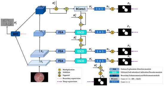
Figure 1. FEBE-Net overall architecture.

Specifically, given an input RGB image $XϵR^{H\times W\times 3}$ to be segmented, due to the stronger ability of Vision Transformer to capture remote dependencies and feature representations compared to the CNN [72], we choose the PVT v2 encoder [28] as the backbone network to capture multi-scale global feature information of bladder tumors to adapt to changes in tumor shape and size. The Transformer backbone PVT v2 extracts four different levels of pyramid features $X_i(i=\mathrm{1,2},\mathrm{3,4})$, where $X_i(i=\mathrm{1,2},3)$ are low-level features that contain more fine-grained detail information, as well as noise information unrelated to bladder tumor segmentation, and $X_4$ is a high-level semantic feature that encompasses richer information for accurately locating bladder tumors. Then, we send the low-level feature $X_i(i=\mathrm{1,2},3)$ to the FEA module to mine potential local detailed feature information of bladder tumors and filter out irrelevant noise, generating the feature maps $O_{{FEA}_i}(i=\mathrm{1,2},3)$. At the same time, we input low-level feature $X_1$ and high-level feature $X_4$ into the BER module to generate high-quality boundary clues $B_f^i$ and replicate four copies to obtain $B_f^4, B_f^3, B_f^2, \mathrm{a}\mathrm{n}\mathrm{d} B_f^1$. Next, the advanced features $X_4$ and boundary clues $B_f^4$ are sent to the decoder.${ B}_f^4$ is first used to enhance the boundary regions in $X_4$, and then a $1\times 1$ convolution unit is used to recover global information to obtain the feature map $D_4^{\prime }$. $D_4^{\prime }$ is then subjected to a $1\times 1$ convolution to decrease the number of channels to 1 to generate the initial global prediction map $D_4$. Then, the ${ O}_{{FEA}_i}(i=\mathrm{1,2},3),{ B}_f^i(i=\mathrm{2,3}), \mathrm{a}\mathrm{n}\mathrm{d} D_{i+1}^{\prime }(i=\mathrm{1,2},3)$ are sent to the proposed decoder module ESCD, and the advanced feature $D_{i+1}^{\prime }(i=\mathrm{2,3})$ is adaptively weighted using the boundary clue $B_f^i(i=\mathrm{2,3})$ to gradually guide the network to focus on the noteworthy bladder tumor boundary region. Through the horizontal connection between the FEA module and the ESCD module, the feature maps $O_{{FEA}_i}(i=\mathrm{1,2},3)$ containing rich local detail information are fused with the advanced feature maps $D_{i+1}^{\prime }(i=\mathrm{1,2},3)$ recovered by the decoder in the previous stage, and a more accurate bladder tumor prediction map $D_i(i=\mathrm{1,2},3)$ is gradually generated through deep decoding. To further refine the boundary areas in the predicted map, we use $B_f^1$ to fine-tune the predicted map $D_1$, achieving complementary feature information between $B_f^1$ and $D_1$, and obtaining a bladder tumor prediction image $D_b$ with clearer and more accurate boundaries. During the experiment, we conducted deep supervision on the bladder tumor prediction maps $D_i(i=\mathrm{1,2},\mathrm{3,4},b)$ output by the decoder in five stages and performed boundary supervision on the generated boundary clues $B_f^i$. Through this hybrid supervision strategy, our FEBE-Net outputs a bladder tumor prediction mask from coarse to fine, ultimately producing a prediction map with accurate localization and clear boundaries. The process can be described as follows:

$$X_i=PVT v2\left(X\right),(i=\mathrm{1,2},\mathrm{3,4})$$

(1)

$$O_{{FEA}_i}=FEA\left(X_i\right)(i=\mathrm{1,2},3)$$

(2)

$$B_f^i=BER(X_1,X_4)$$

(3)

$${ D}_4^{\prime }=BConv1(X_4+B_f^4\times X_4)$$

(4)

$${ D}_i^{\prime }=ESCD(O_{{FEA}_i},({ D}_{i+1}^{\prime }+B_f^i\times { D}_{i+1}^{\prime }\left)\right)(i=\mathrm{2,3})$$

(5)

$${ D}_1^{\prime }=ESCD(O_{{FEA}_1},{ D}_2^{\prime })$$

(6)

$$D_i=Conv1\left(D_i^{\prime }\right),(i=\mathrm{1,2},\mathrm{3,4})$$

(7)

$$D_b=D_1+B_f^1$$

(8)

3.2. Feature Exploration Attention Module (FEA)

Since the low-level features $X_i(i=\mathrm{1,2},3)$ extracted by the PVT v2 encoder contain rich detailed information, it is possible to explore and focus on these features to solve the problem of high-level features losing local detail feature information and small bladder tumors. However, these low-level features contain more background noise and irrelevant information, and there is a semantic gap between them and high-level features. Therefore, we propose a new feature exploration attention module (FEA) aimed at extracting local fine-grained detail information from low-level features while filtering noise, and then supplementing the captured fine-grained detail information to the corresponding high-level features at the decoder end through horizontal connections, bridging semantic gaps.

The structure of the proposed feature exploration attention module (FEA) is shown in Figure 2. Specifically, FEA has four branches, each of which performs different convolution operations on low-level features $X_i(i=\mathrm{1,2},3)$ to capture local information. Among them, the first branch uses a $3\times 3$ convolution unit with an expansion rate of 1 for feature mining; on this basis, the second branch adds a $3\times 3$ convolution unit with an expansion rate of 3 for subsequent feature exploration; similarly, the third branch supplements and explores features through three $3\times 3$ convolution units with expansion rates of 1, 3, and 5, respectively; then, the outputs of the first three branches are concatenated to expand the receptive field and more effectively identify large bladder tumors. Next, a $1\times 1$ convolution is used to reduce the number of channels and computational resources. Unlike the first three branches, the fourth branch uses self-calibrated convolution [53] to capture richer detailed features to enhance the recognition of small bladder tumors and then performs concatenation operations to help enhance features and capture fine-grained detailed features. Subsequently, we utilized the LECA module [34] to filter out noise, purify feature information, and force the network to focus on feature information closely related to bladder tumor segmentation. Finally, we used a $3\times 3$ convolution unit to further denoise the features and restore them to the original number of channels. In this way, the FEA module can explore potential local detailed feature information of bladder tumors and enhance feature representation. The process can be described as follows:

$$F_{11}=DConv1\left(X_i\right),(i=\mathrm{1,2},3)$$

(9)

$$F_{12}=DConv3\left(DConv1\right(X_i\left)\right),(i=\mathrm{1,2},3)$$

(10)

$$F_{13}=DCon5\left(DConv3\right(DConv1\left(X_i\right)\left)\right),(i=\mathrm{1,2},3)$$

(11)

$$F_1=Conv1\left(Cat\right(F_{11},F_{12},F_{13}\left)\right)$$

(12)

$$F_2={Conv}_{sc}\left(X_i\right),(i=\mathrm{1,2},3)$$

(13)

$$O_{{FEA}_i}=BConv3\left(LECA\right(Cat(F_1,F_2)\left)\right)$$

(14)

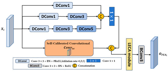
Figure 2. Structure of feature exploration attention module (FEA).

In the above equation, $DConvi(i=\mathrm{1,3},5)$ represent a $3\times 3$ convolution with dilation rates of 1, 3, and 5, Batch Normalization, and PReLU activation functions, respectively. $Cat(·)$ represents a concatenation operation in the channel dimension, $Conv1(·)$ represents $1\times 1$ convolution, ${Conv}_{sc}$ represents the self-calibrated convolution, and $BConv3$ represents $3\times 3$ convolution, Batch Normalization, and ReLU activation functions.

3.3. Efficient Self-Attention Calibration Decoder Module (ESCD)

High-level features typically contain more semantic information that can identify target regions; however, they may lose some bladder tumor details or small bladder tumors, which are difficult to recover at the decoder end. Therefore, we propose a new efficient self-attention calibration decoder module (ESCD) that combines the fine-grained detail information captured by the FEA module in low-level features with the global semantic information in corresponding high-level features, effectively restoring local tumor feature details while achieving accurate bladder tumor localization.

The structure of the proposed efficient self-attention calibration decoder module (ESCD) is shown in Figure 3. Firstly, we use a convolutional layer with a stride of 4 and a kernel size of 7 to embed the high-level features into overlapping patches and model the local continuity information by combining the information of each patch with the information of adjacent patches in the top, bottom, left, and right directions. Then, the obtained serialization tokens are processed through three parallel fully connected layers to compute the query Q, key K, and value V. Next, we calculate the similarity between Q and K to obtain the affinity matrix ${QK}^T$, which is then scaled by dividing it by $\sqrt{d_k}$ to avoid the gradient vanishing or exploding during the subsequent normalization process using the Softmax function. Finally, we multiply the obtained weights $Softmax\left({\displaystyle \frac{{QK}^T}{\sqrt{d_k}}}\right)$ and value V to obtain the output $O_{SRA}$, which can be described by Equation (7):

$$O_{SRA}=Softmax\left({\displaystyle \frac{{QK}^T}{\sqrt{d_k}}}\right)V$$

(15)

where $\sqrt{d_k}$ represents the dimension of the feature embedding. $O_{SRA}$ is added to V and then input into the Convolutional Feed Fold module (CFF) for further decoding to obtain the output $O_{CFF}$. This process can be described by Equations (16) and (17):

$$O_{CFF}=O_{SRA}+V+CFF{(O}_{SRA}+V)$$

(16)

$$CFF\left(x\right)=fc2\left(R\right(DWConv\left(fc1\right(x\left)\right)\left)\right)$$

(17)

where $x$ is the input feature, $fc1$ and $fc2$ are linear fully connected mapping layers with a dilation rate of 4, $DWConv(·)$ is a deep convolutional layer used to model position information and reduce computational complexity, and $R(·)$ represents the ReLU activation function.

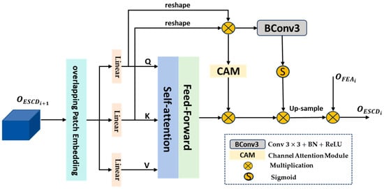
Figure 3. Structure of efficient self-attention calibration decoder module (ESCD).

Due to the inherent contextual statistical information carried by Q and K, we multiply them to obtain the fused feature $Q^r{K}^r$, which is calibrated through two branches to extract more valuable contextual key information. Then, the outputs of the two calibration branches are sequentially multiplied with $O_{CFF}$ to enhance global features and eliminate noise. Among them, the first branch is the channel attention module (CAM) [54], and the second branch is the convolutional attention module, which consists of a $3\times 3$ convolution unit and a Sigmoid function. Due to the similarity of K and V, these two branches can, respectively, weaken irrelevant contextual information from the channel dimension and spatial dimension. This process can be described using Formulas (18)–(20):

$$Q^r{K}^r=r\left(Q\right)\times r\left(K\right)$$

(18)

$$O_{CFF1}=CAM\left(Q^r{K}^r\right)\times O_{CFF}$$

(19)

$$O_{CFF2}=S\left(BConv3\right(Q^r{K}^r\left)\right)\times O_{CFF1}$$

(20)

where $r(·)$ represents the reshape operation; $BConv3$ represents the $3\times 3$ convolution, Batch Normalization, and ReLU activation function; and $S(·)$ represents the Sigmoid activation function.

Then, the globally enhanced feature $O_{CFF2}$ after calibration is upsampled and multiplied with the fine-grained detail feature $O_{{FEA}_i}$ output by the FEA module to continuously supplement rich local detail features, which helps the decoder module restore fine-grained details when predicting bladder tumor areas and output accurate high-resolution bladder tumor prediction masks. This process can be described using Formula (21):

$$O_{{ESCD}_i}= Up\_sample\left(O_{CFF2}\right)\times O_{{FEA}_i}$$

(21)

3.4. Boundary Enhancement and Refinement Module (BER)

Boundary feature information can help enhance the learning ability of medical image semantic segmentation [36,73]. Therefore, we propose a new boundary enhancement and refinement module (BER) that directly utilizes the first- and fourth-layer features extracted by the encoder to generate high-quality boundary clues, which are then integrated into the bladder tumor prediction task. The aim is to enhance the boundary regions in the high-level features during the decoding stage and fine-tune the final predicted feature map, making the network generate more accurate localization and clearer boundary prediction masks.

The structure of the proposed boundary enhancement and refinement module (BER) is shown in Figure 4. We extract boundary feature information from low-level feature $X_1$ and high-level feature $X_4$ and filter out boundary-irrelevant information.

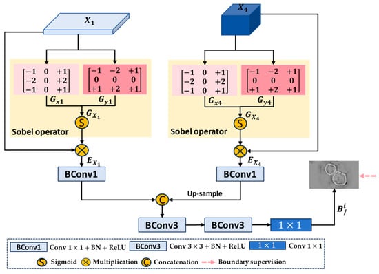
Figure 4. Structure of boundary enhancement and refinement module (BER).

Firstly, we use the Sobel operator to calculate the gradients of low-level feature $X_1$ and high-level feature $X_4$ in the horizontal and vertical directions, respectively, to obtain gradient maps $G_{X_1}$ and $G_{X_4}$ in the overall direction. Specifically, taking low-level feature $X_1$ as an example, the convolutions $C_{x1}$ and $C_{y1}$ in the horizontal and vertical directions are defined as

$$C_{x1}=\left[\begin{array}{ccc}-1& 0& 1\\ -2& 0& 2\\ -1& 0& 1\end{array}\right], C_{y1}=\left[\begin{array}{ccc}-1& -2& -1\\ 0& 0& 0\\ 1& 2& 1\end{array}\right]$$

(22)

Then, $X_1$ is convolved with $C_{x1}$ and $C_{y1}$, respectively, to obtain gradient maps $G_{x1}$ and $G_{y1}$ in the horizontal and vertical directions, and $G_{x1}$ and $G_{y1}$ are used to obtain gradient map $G_{X_1}$ in the overall direction:

$$G_{X_1}=\sqrt{{G_{x1}}^2+{G_{y1}}^2}$$

(23)

Next, the gradient map $G_{X_1}$ is normalized using the Sigmoid activation function and then multiplied with the original feature $X_1$ to obtain the boundary-enhanced feature map $E_{X_1}$. For the high-level feature $X_4$, the same can be applied to obtain its boundary-enhanced feature map $E_{X_4}$:

$$E_{X_1}=S\left(G_{X_1}\right)\times X_1$$

(24)

$$E_{X_4}=S\left(G_{X_4}\right)\times X_4$$

(25)

In Equations (24) and (25), $S(·)$ represents the Sigmoid activation function.

Then, we perform a series of convolution fusion operations on the boundary-enhanced feature maps $E_{X_1}$ and $E_{X_4}$. Specifically, we use two $1\times 1$ convolution units to reduce the number of channels in $E_{X_1}$ and $E_{X_4}$ to 32, further extracting features while reducing computational resource consumption. Then, bilinear upsampling operation is used to adjust the size of $E_{X_4}$ to be the same as $E_{X_1}$. The two are further concatenated and fused along the channel dimension, boundary information is extracted, irrelevant noise is eliminated through two consecutive $3\times 3$ convolution units, and the number of channels is finally reduced to 1 through a convolution layer with a kernel size of 1 to generate a bladder tumor boundary prediction feature map $B_f^i$. This process can be described by the following formula:

$${E_{X_1}}^{\prime }=BConv1\left(E_{X_1}\right)$$

(26)

$${E_{X_4}}^{″}=Up\_sample\left(BConv1\right(E_{X_4}\left)\right)$$

(27)

$$B_f^i=Conv1\left(BConv3\right(BConv3\left(Cat\right({E_{X_1}}^{\prime },{E_{X_4}}^{″}\left)\right)\left)\right))$$

(28)

where $BConv1$ represents $1\times 1$ convolution, Batch Normalization, and ReLU activation functions. $Cat(·)$ represents concatenation operation in the channel dimension. $BConv3$ represents $3\times 3$ convolution, Batch Normalization, and ReLU activation functions. $Conv1(·)$ represents $1\times 1$ convolution.

In addition, we apply the same Sobel operator to each bladder tumor mask in the ground truth map (GT) to generate the corresponding tumor boundary mask, obtaining the ground truth boundary map (GTB). By using the GTB for the boundary supervision of $B_f^i$, we can eliminate the internal edge feature information of bladder tumors and obtain high-quality bladder tumor boundary clues.

We copy the output bf of the BER module into four copies: $B_f^4,{ B}_f^3,{ B}_f^2, B_f^1$. The input features $X_4,{ D}_4{, \mathrm{a}\mathrm{n}\mathrm{d} D}_3$ in the first three layers in the decoding stage contain more advanced semantic concepts, but there is no clear boundary between their foreground and background; therefore, we integrate $B_f^4, { B}_f^3, { B}_f^2$ into the high-level features $X_4, D_4{, D}_3$. Specifically, we use downsampling operations to adjust the size of boundary clues $B_f^4,{ B}_f^3,{ \mathrm{a}\mathrm{n}\mathrm{d} B}_f^2$ to be the same as $X_4, D_4{,\mathrm{a}\mathrm{n}\mathrm{d} D}_3$. Then, we multiply the downsampled boundary clue maps with $X_4, D_4{, \mathrm{a}\mathrm{n}\mathrm{d} D}_3$ and add the multiplication results to $X_4,{ D}_4{, \mathrm{a}\mathrm{n}\mathrm{d} D}_3$ to enhance the boundary regions in these high-level features. The aim is to gradually guide the network to focus on noteworthy boundary regions and generate more accurate bladder tumor prediction maps. In addition, we also use $B_f^1$ to fine-tune the final predicted feature map, achieving feature information complementarity and further refining the bladder tumor prediction map.

3.5. Overall Loss Function

As shown in Figure 1, our proposed FEBE-Net requires the ground truth map (GT) and ground truth boundary map (GTB) to supervise the bladder tumor prediction mask $D_i(i=\mathrm{1,2},\mathrm{3,4},b)$ and tumor boundary prediction mask $B_f^i$, respectively. Therefore, we designed a mixed supervision strategy and defined an overall loss function $L_{overall}$ to optimize the network:

$$L_{overall}=\sum _{i=1}^4{L_{seg}}_i+L_{{seg}_b}+\omega L_{bnd}$$

(29)

$$L_{{seg}_i}= L_{wiou}(D_i,GT)+L_{wbce}(D_i,GT) (i=\mathrm{1,2},\mathrm{3,4},b)$$

(30)

$$L_{bnd }= L_{Dice}(B_f^i,GTB)$$

(31)

$$L_{Dice}=1-{\displaystyle \frac{2\sum _{i=1}^N(g_i\times p_i)}{\sum _{i=1}^N(g_i+p_i)}}$$

(32)

where $L_{{seg}_i}(i=\mathrm{1,2},\mathrm{3,4},b)$ stands for the loss function for bladder tumor segmentation in 5 stages, which consists of wiou loss [74] and wbce loss [74], where wiou [74] and wbce [74] constrain the segmentation results of bladder tumors from global and local perspectives, respectively. $L_{bnd}$ stands for the bladder tumor boundary segmentation loss function, which uses the Dice loss function to alleviate the negative impact of area imbalance between foreground and background pixels in boundary segmentation. N represents the total number of pixels in the cystoscopy image, and $g_i$ and $p_i$ represent the ground truth and predicted label of the ith pixel, respectively. $\omega$ is a weight factor that balances segmentation loss and boundary segmentation loss, which is set to 5 in this paper.

In addition, we provide details of the process of the training of the proposed algorithm FEBE-Net, as shown in Algorithm 1.

Algorithm 1: FEBE-Net training process.

Input: Image set $I_1$, ${ I}_2$, … $I_n$, Label(image ground truth) set $G_1$, $G_2$, … $G_n$

Output: Segmentation maps $D_i$, Model parameters $\mathrm{\varnothing }$

1:  While not converging do

2:   Sample $I_i$, ${\hspace{1em}G}_i$ from $I_1$, ${\hspace{1em}I}_2$, … $I_n$, $G_1$, $G_2$, … $G_n$

3:   Obtain pyramid feature maps at four distinct levels. $X_1$, $X_2$, $X_3$, $X_4=\hspace{1em}Transformer\hspace{1em}Backbone-PVT\hspace{1em}v2\left(I_i\right)$

4:   for feature maps $X_i$ do

5:    for $i=1$ to 3 do

6:      Extract local detailed features and filter out noise $O_{{FEA}_i}=FEA\left(X_i\right)$

7:    end for

8:  end for

9:   Generate high-quality boundary clues $B_f^i=BER(X_1,X_4)$

10:  Copy 4 copies of boundary clues $B_f^i$: $B_f^4,\hspace{1em}{B}_f^3,{\hspace{1em}B}_f^2,\hspace{1em}{\hspace{1em}B}_f^1$

11:  Enhance the boundary regions in feature map $X_4$ and generate initial global feature map $D_4^{\prime }$ by Equation (4)

12:  for feature maps $D_i^{\prime }$, $B_f^i$, $O_{{FEA}_i}$ do

13:   for $i=1$ to 3 do

14:    if $i=2$ or 3 do

15:     Enhance the boundary regions in feature maps $D_{i+1}^{\prime }={\hspace{1em}D}_{i+1}^{\prime }+B_f^i\times {\hspace{1em}D}_{i+1}^{\prime }$

16:     Continuously restore global features and supplement rich local detail Features: $D_i^{\prime }=ESCD(O_{{FEA}_i},{\hspace{1em}D}_{i+1}^{\prime })$

17:   end for

18:  end for

19:  for feature maps $D_i^{\prime }$ do

20:   for $i=1$ to 4 do

21:    Use Equation (10) to generate prediction maps $D_i$

22:   end for

23:  end for

24:  Refine the boundary regions in the prediction map $D_1$:${\hspace{1em}D}_b=D_1+B_f^1$

25:  Use Equations (29)–(32) to calculate the overall loss $L_{overall}$

26:  Use the Adam optimizer and the loss function $L_{overall}$ to update the network parameters $\mathrm{\varnothing }$

27: end while

4. Results and Discussion

4.1. Experimental Datasets

To comprehensively evaluate the performance of our proposed FEBE-Net network model in bladder tumor segmentation tasks, we selected the BtAMU [55] dataset consisting of bladder tumor images extracted from cystoscopy videos. In addition, we also selected five publicly available polyp datasets, all of which were sourced from colonoscopy videos, to validate the robustness and generalization ability of FEBE-Net. The specific information of the dataset is shown in Table 1. We randomly selected 1562 image data points from BtAMU [55] for training and tested the remaining 386 image data points for bladder tumor segmentation experiments. In the polyp segmentation experiment, we used the same data settings as PraNet to randomly select 900 and 550 polyp images from Kvasir-SEG [56] and CVC-ClinicDB [57] for model training. The remaining 100 and 62 images from Kvasir-SEG [56] and CVC-ClinicDB [57] were used to test the model’s learning ability, respectively. In addition, all images from CVC-ColonDB [58], ETIS [59], and CVC-300 [60] were not involved in training the model and were only used to test the model’s generalization ability.

Table 1. Detailed information on the experimental datasets and the configuration of training and testing data.

Dataset	Target	Image Source	Resolution	Total	Train	Test
BtAMU [55]	Bladder tumor	cystoscopy	$1920\times 1080$	1948	1562	386
Kvasir-SEG [56]	polyp	colonoscopy	Variable	1000	900	100
CVC-ClinicDB [57]	$\mathrm{polyp}$	$\mathrm{colonoscopy}$	$384\times 288$	612	550	62
CVC-ColonDB [58]	$\mathrm{polyp}$	$\mathrm{colonoscopy}$	$574\times 500$	380	0	380
ETIS [59]	$\mathrm{polyp}$	$\mathrm{colonoscopy}$	$1225\times$996	196	0	196
CVC-300 [60]	$\mathrm{polyp}$	$\mathrm{colonoscopy}$	$574\times 500$	60	0	60

4.2. Evaluation Metrics

We chose eight widely used medical image segmentation evaluation metrics to quantitatively assess the performance of the proposed FEBE-Net against other 11 state-of-the-art (SOTA) models, including the mean Dice (mDice), mean Intersection over Union (mIoU), mean absolute error (MAE), structure measure ($S_{\alpha }$), enhanced-alignment measure ($E_{\phi }$), accuracy and weighted F-measure ($F_{\beta }^{\omega }$), and Hausdorff distance (HD). Specifically, mDice and mIoU are used to quantify the extent of overlap between the predicted regions and the true regions; MAE is used to compare the pixel-by-pixel absolute value difference between the Predicted map (P) and Ground Truth (G); $S_{\alpha }$ is used to evaluate the structural similarity between predicted results and actual results; $E_{\phi }$ evaluates the prediction results at both pixel and image levels; Accuracy represents the proportion of pixels correctly predicted by the network to the total number of pixels in the image; $F_{\beta }^{\omega }$ is used to calculate the weighted sum average of $\mathrm{P}\mathrm{r}\mathrm{e}\mathrm{c}\mathrm{i}\mathrm{s}\mathrm{i}\mathrm{o}\mathrm{n}$ and $\mathrm{R}\mathrm{e}\mathrm{c}\mathrm{a}\mathrm{l}\mathrm{l}$; and HD is used to evaluate the accuracy of boundary segmentation. Among these metrics, the closer the values of mDice, mIoU, $S_{\alpha }{, E}_{\phi }$, Accuracy, and $F_{\beta }^{\omega }$ are to 1, the better the segmentation effect; the closer the MAE value is to 0, the better the segmentation effect; and the lower the HD value, the better the segmentation effect. The definitions of these indicators are as follows:

$$mDice={\displaystyle \frac{1}{N+1}}\sum _{i=0}^N{\displaystyle \frac{2TP}{FP+2TP+FN}}$$

(33)

$$mIoU={\displaystyle \frac{1}{N+1}}\sum _{i=0}^N{\displaystyle \frac{TP}{FP+TP+FN}}$$

(34)

$$MAE={\displaystyle \frac{1}{W\times H}}\sum _{x=1}^W\sum _{y=1}^H\left|P\right(x,y)-G(x,y\left)\right|$$

(35)

$$S_{\alpha }=(1-\alpha )\times S_o(P,G)+\alpha \times S_r(P,G)$$

(36)

$$E_{\phi }={\displaystyle \frac{1}{W\times H}}\sum _{x=1}^W\sum _{y=1}^H\phi \left(P\right(x,y)-G(x,y\left)\right)$$

(37)

$$Accuracy={\displaystyle \frac{TP+TN}{TP+TN+FP+FN}}$$

(38)

$$\left\{\begin{array}{c}Precision={\displaystyle \frac{TP}{FP+TP}}\\ Recall={\displaystyle \frac{TP}{TP+FN}}\\ F_{\beta }^{\omega }={\displaystyle \frac{({\beta }^2+1){Precision}^{\omega }·{Recall}^{\omega }}{{\beta }^2·{Precision}^{\omega }+{Recall}^{\omega }}}\end{array}\right.$$

(39)

$$\left\{\begin{array}{c}h\left(A,B\right)={max}_{a\in A} {min}_{b\in B}‖a-\mathrm{b}‖\\ HD\left(A,B\right)={\displaystyle \frac{1}{N+1}}{\displaystyle \sum _{i=0}^N}max\left(h\left(A,B\right),h\left(B,A\right)\right)\end{array}\right.$$

(40)

where TP stands for True Positive, TN denotes True Negative, FP refers to False Positive, and FN indicates False Negative. Additionally, N represents the total number of test images. In Formulas (34) and (36), W and H are the width and height of images, respectively. In Formula (35), $\alpha$ is the coefficient used to balance the object-level similarity $S_o$ with the region-level similarity $S_r$. In Formula (36), $\phi$ is the enhanced alignment matrix. In Formula (37), $\omega$ is a weight coefficient that balances weighted Precision and weighted Recall, which is set to 1 in this paper. In Formula (39), A and B denote the true image and the predicted map, and $‖a-\mathrm{b}‖$ denotes a distance function.

4.3. Implementation Details

FEBE-Net is implemented using Python 3.7 and the PyTorch 1.7.1 framework. The model training and evaluation are conducted on an NVIDIA GeForce RTX 3090 GPU with 24 GB VRAM. We initialize the PVT v2 [28] backbone using pre-trained Transformer weights from ImageNet [61] to accelerate the network convergence process. During training, the batch size is set to 8, the optimizer is set to Adam, the initial learning rate is set to ${5\times 10}^{-5}$, the decay rate is set to 0.1, and the model trains 100 epochs. To accelerate the convergence process of the model, the learning rate is stepped down with a decay rate of 0.5 after the 15th and 30th epochs. Additionally, we adjust the resolution of the image to be segmented to $352\times 352$ and use a multi-scale training strategy to reduce the model’s sensitivity to scale changes.

4.4. Results and Discussion on the Bladder Tumor Dataset

4.4.1. Quantitative Analysis

To verify the effectiveness and superiority of the proposed FEBE-Net in segmenting bladder tumors in cystoscopic images, we compared it with 11 state-of-the-art (SOTA) methods, including the quantitative experimental results of U-Net [10], PraNet [14], HarDNet-MSEG [16], Polyp-PVT [32], CaraNet [17], DCRNet [18], MSRAformer [31], HSNet [34], TMUnet [47], TGDAUNet [44], and MSGAT [38]. Table 2 shows the quantitative results of the proposed FEBE-Net and 11 other SOTA methods on the bladder tumor dataset BT-AMU [55]. As shown in Table 2, our FEBE-Net outperforms other SOTA methods in all evaluation metrics (mDice, mIoU, MAE, $S_{\alpha }$, $E_{\phi }$, Accuracy, $F_{\beta }^{\omega }$, and HD). For example, our FEBE-Net is much better than the classic medical image segmentation method U-Net [10], leading U-Net [10] by 8.6% and 10.05% in mDice and mIoU metrics, respectively, and achieving similar leading results in other metrics. For mDice, mIoU, and $E_{\phi }$ metrics, our FEBE-Net achieved improvements of 1.01%, 1.4%, and 0.44%, respectively, when compared to the second-best-performing MSGAT [38]. For MAE and HD indicators, the proposed FEBE-Net showed a decrease of 0.17% and 0.348% compared to the second-best-performing HSNet [34] and MSGAT [38], respectively. In addition, $S_{\alpha }$, Accuracy, and $F_{\beta }^{\omega }$ indicator values lead the second-best-performing MSRAformer [31] by 0.44%, 0.16%, and 0.52%, respectively. These quantitative comparison results indicate that our FEBE-Net is more accurate in segmenting bladder tumors in cystoscopy images and can provide higher segmentation accuracy, verifying the effectiveness and superiority of the proposed FEBE-Net.

Table 2. Comparison of quantitative results of different methods on the BT-AMU [55] dataset; ↑ indicates that the higher the value, the better; ↓ indicates that the lower the value, the better; and the bolded values represent the best performance results.

Methods	mDice ↑	mIoU ↑	MAE ↓	${\mathit{S}}_{\mathit{\alpha }}$ ↑	${\mathit{E}}_{\mathit{\phi }}$ ↑	Accuracy ↑	${\mathit{F}}_{\mathit{\beta }}^{\mathit{\omega }}$ ↑	HD ↓
U-Net [10]	0.8266	0.7573	0.0271	0.8612	0.9140	0.9729	0.9043	11.8904
PraNet [14]	0.8680	0.8092	0.0239	0.8986	0.9370	0.9774	0.9305	11.1110
HarDNet-MSEG [16]	$0.8613$	$0.8001$	0.0250	0.8899	0.9382	0.9763	0.9213	11.2059
Polyp-PVT [32]	$0.9014$	$0.8417$	0.0213	0.9085	0.9582	0.9788	0.9449	10.7594
CaraNet [17]	$0.8253$	$0.7641$	0.0385	0.8733	0.8967	0.9664	0.9147	12.2071
DCRNet [18]	$0.8695$	$0.8096$	0.0240	0.8975	0.9408	0.9771	0.9281	11.3585
MSRAformer [31]	$0.9008$	$0.8414$	0.0201	0.9121	0.9552	0.9809	0.9460	10.7913
HSNet [34]	$0.9011$	$0.8412$	0.0192	0.9068	0.9600	0.9808	0.9455	10.7512
TMUnet [47]	$0.8941$	$0.8335$	0.0214	0.9066	0.9573	0.9788	0.9405	10.8318
TGDAUNet [44]	0.8951	0.8330	0.0202	0.9034	0.9585	0.9798	0.9451	10.7861
MSGAT [38]	0.9025	0.8438	0.0201	0.9087	0.9591	0.9799	0.9446	10.6468
FEBE-Net	0.9126	0.8578	0.0175	0.9165	0.9635	0.9825	0.9512	10.2988

4.4.2. Qualitative Analysis

To more intuitively evaluate the proposed FEBE-Net, we compared it with 11 state-of-the-art (SOTA) methods, including the visual qualitative experimental results of U-Net [10], PraNet [14], HarDNet-MSEG [16], Polyp-PVT [32], CaraNet [17], DCRNet [18], MSRAformer [31], HSNet [34], TMUnet [47], TGDAUNet [44], and MSGAT [38]. Figure 5 shows a comparison of the qualitative experimental results between the proposed FEBE-Net and 11 SOTA methods on the bladder tumor dataset BT-AMU. As shown in Figure 5, compared to 11 SOTA methods, our FEBE-Net achieves significantly more accurate segmentation results in various backgrounds. In the first column of Figure 5, TGDAUNet [44] shows prominent errors when predicting bladder tumors, failing to identify the bladder tumor area and mistakenly classifying normal tissue as bladder tumors; the other comparison methods also struggle to accurately delineate the boundaries, whereas our FEBE-Net successfully identifies the bladder tumor area while accurately delineating the boundaries. In the second column of Figure 5, our FEBE-Net demonstrates an advantage in precisely locating small tumors; U-Net [10] fails to recognize the small tumor area, HSNet [34] can predict the small tumor but contains an incorrect tumor prediction area, while other methods exhibit varying degrees of over-segmentation and under-segmentation. The bladder wall backgrounds in Figure 5c,d contain normal fold regions; compared to other SOTA methods, the proposed FEBE-Net is better suited for predicting bladder tumors from these complex backgrounds, showcasing strong robust stability. Additionally, in low-light images (Figure 5e), the prediction result from FEBE-Net remains closest to the ground truth (GT) image. Overall, the proposed FEBE-Net adapts well to variations in size and morphology of bladder tumors (Figure 5a–e), small bladder tumors (Figure 5b), folds in the background (Figure 5c,d), and low light conditions (Figure 5e), consistently predicting accurate bladder tumor regions with clear boundaries. The comparison of visual qualitative results once again validates the effectiveness, robust stability, and superiority of the proposed FEBE-Net.

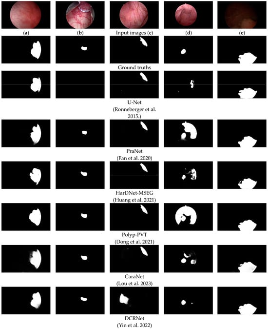
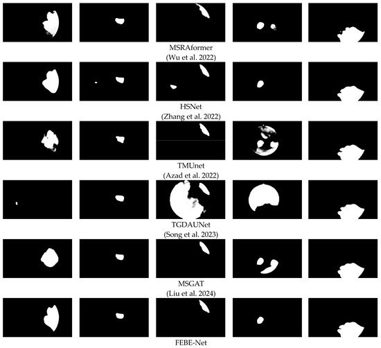
Figure 5. Comparison of visual qualitative results of different methods on the BT-AMU [55] dataset. From the first line to the last line are the input images, ground truths (GTs), and the predicted results of U-Net [10], PraNet [14], HarDNet-MSEG [16], Polyp-PVT [32], CaraNet [17], DCRNet [18], MSRAformer [31], HSNet [34], TMUnet [47], TGDAUNet [44], MSGAT [38], and our proposed FEBE-Net.

4.5. Results and Discussion on Polyp Datasets

To verify the robustness and generalization of the proposed FEBE-Net, we conducted experimental comparisons with U-Net [10], UNet++ [11], PraNet [14], HarDNet-MSEG [16], TransUNet [40], DCRNet [18], MSRAformer [31], SSFormer [29], TMUnet [47], TGDAUNet [44], and MSGAT [38] on five publicly available polyp datasets. Table 3 shows the quantitative results of our FEBE-Net and 11 other SOTA methods on the polyp datasets Kvasir-SEG [56] and CVC-ClinicDB [57]. As shown in Table 3, our FEBE Net outperforms other state-of-the-art techniques in the evaluation metrics mDice and mIoU on both datasets. Among them, on the CVC-ClinicDB [57] dataset, FEBE-Net’s mDice and mIoU values are 1.62% and 1.84% higher than those of the second-best-performing MSGAT [38], respectively. This indicates that FEBE-Net has stronger feature modeling capabilities than other SOTA methods. Table 4 shows the quantitative results of our FEBE-Net compared to 11 other state-of-the-art methods on three unseen (not involved in model training) polyp datasets: CVC-ColonDB [58], ETIS [59], and CVC-300 [60]. As shown in Table 4, the segmentation accuracy of FEBE-Net is consistently superior to other SOTA methods. Specifically, on the CVC-ColonDB [58] dataset, compared to the second-best-performing MSGAT [38], the mDice and mIoU values of FEBE-Net increased by 1.04% and 0.96%, respectively. On the ETIS dataset, FEBE-Net’s mDice and mIoU values lead the second-best-performing MSGAT [38] by 2.62% and 2.35%, respectively, and lead the third-ranked MSRAformer [31] by 3.18% and 2.31%, respectively; because the smallest polyps in the ETIS [59] dataset cannot be accurately identified by the naked eye, ETIS [59] is more challenging. On the CVC-300 [60] dataset, FEBE-Net’s mIoU value improved by 0.97% and 2.46%, respectively, compared to the second-best-performing MSGAT [38] and the third-ranked TGDAUNet [44]. This indicates that FEBE-Net has a stronger generalization ability, especially on the challenging small-polyp dataset ETIS [59]. Overall, FEBE-Net demonstrated the strongest segmentation performance on all five polyp datasets, confirming its robustness and generalization ability.

Table 3. Comparison results of different methods on Kvasir-SEG [56] and CVC-ClinicDB [57] datasets; ↑ indicates that the higher the value, the better; the bolded values represent the best performance results.

Datasets	Methods	mDice ↑	mIoU ↑
Kvasir-SEG [56]	U-Net [10]	0.8209	0.7559
	UNet++ [11]	0.8237	0.7532
	PraNet [14]	0.9005	0.8475
	HarDNet-MSEG [16]	0.8991	0.8434
	TransUNet [40]	0.8849	0.8127
	DCRNet [18]	0.8881	0.8384
	MSRAformer [31]	0.9090	0.8604
	SSFormer [29]	0.8463	0.7566
	TMUnet [47]	0.9144	0.8574
	TGDAUNet [44]	0.9207	0.8699
	MSGAT [38]	0.9226	0.8734
	FEBE-Net	0.9236	0.8759
CVC-ClinicDB [57]	U-Net [10]	0.8243	0.7668
	UNet++ [11]	0.7970	0.7412
	PraNet [14]	0.9016	0.8576
	HarDNet-MSEG [16]	0.9124	0.8670
	TransUNet [40]	0.8679	0.8152
	DCRNet [18]	0.8987	0.8565
	MSRAformer [31]	0.9175	0.8715
	SSFormer [29]	0.8291	0.7496
	TMUnet [47]	0.8945	0.8370
	TGDAUNet [44]	0.9213	0.8689
	MSGAT [38]	0.9280	0.8808
	FEBE-Net	0.9442	0.8992

Table 4. Comparison results of different methods on CVC-ColonDB [58], ETIS [59], and CVC-300 [60] datasets; ↑ indicates that the higher the value, the better; the bolded values represent the best performance results.

Datasets	Methods	mDice ↑	mIoU ↑
CVC-ColonDB [58]	U-Net [10]	0.5113	0.4402
	UNet++ [11]	0.4894	0.4111
	PraNet [14]	0.7161	0.6449
	HarDNet-MSEG [16]	0.7384	0.6686
	TransUNet [40]	0.7065	0.6385
	DCRNet [18]	0.7069	0.6418
	MSRAformer [31]	0.8048	0.7292
	SSFormer [29]	0.6966	0.6966
	TMUnet [47]	0.7378	0.6618
	TGDAUNet [44]	0.7743	0.7034
	MSGAT [38]	0.8195	0.7418
	FEBE-Net	0.8299	0.7514
ETIS [59]	U-Net [10]	0.4059	0.3430
	UNet++ [11]	0.4134	0.3420
	PraNet [14]	0.6300	0.5757
	HarDNet-MSEG [16]	0.7029	0.6343
	TransUNet [40]	0.7092	0.6284
	DCRNet [18]	0.5495	0.5064
	MSRAformer [31]	0.7844	0.7165
	SSFormer [29]	0.5567	0.5567
	TMUnet [47]	0.7442	0.6568
	TGDAUNet [44]	0.7600	0.6789
	MSGAT [38]	0.7934	0.7161
	FEBE-Net	0.8161	0.7396
CVC-300 [60]	U-Net [10]	0.7166	0.6390
	UNet++ [11]	0.7144	0.6362
	PraNet [14]	0.8727	0.8039
	HarDNet-MSEG [16]	0.8771	0.8081
	TransUNet [40]	0.8271	0.7310
	DCRNet [18]	0.8580	0.7974
	MSRAformer [31]	0.8765	0.9068
	SSFormer [29]	0.7908	0.7005
	TMUnet [47]	0.8522	0.7634
	TGDAUNet [44]	0.8730	0.8084
	MSGAT [38]	0.8920	0.8233
	FEBE-Net	0.8991	0.8330

4.6. Ablation Studies

To validate the effectiveness of the three new modules FEA, ESCD, and BER in the proposed network architecture FEBE-Net, we conduct ablation experiments on the bladder tumor dataset BT-AMU [55] to verify the effectiveness of each module and explore its contribution to the overall performance of the network model.

Specifically, our baseline retains the PVT v2 [28] backbone network and removes three modules, FEA, ESCD, and BER, and we construct the most basic decoder module by using one $1\times 1$ convolution unit and bilinear upsampling operation; to verify the effectiveness of the FEA module, we directly remove it from FEBE-Net. For the ESCD module, we replace it with one $1\times 1$ convolutional unit and perform bilinear upsampling operation to reconstruct the decoder for comparative verification. For the BER module, we directly remove it for comparative verification. In Table 5, we label the ablation experiments of the FEA, ESCD, and BER modules as “no FEA”, “no ESCD”, and “no BER”, respectively. As shown in Table 5, the mDice and mIoU values of “no FEA” decreased by 1.37% and 2.18%, respectively, compared to FEBE-Net. This indicates that the potential local detail information in the low-level features explored and mined by the FEA module can supplement the missing fine-grained details in the subsequent decoding stage and improve the network segmentation performance. The mDice and mIoU indicators of “no ESCD” decreased by 1.37% and 1.95%, respectively, compared to FEBE-Net. This is because the ESCD module can continuously fuse the local detail features after exploration and attention with the calibrated and enhanced global features, more effectively restoring global contextual information and local detail information. In terms of mDice and mIoU indicators, the “no BER” decreased by 0.76% and 1.01%, respectively, compared to FEBE-Net, while the HD value increased by 0.3696. This indicates that the boundary clues provided by the BER module not only improve the learning ability of the semantic segmentation of bladder tumors but also help generate more accurate prediction masks for boundaries. We also designed a histogram to visually represent the ablation study results on the bladder tumor dataset BT-AMU [55], as shown in Figure 6. From Table 5 and Figure 6, it can be seen that compared to FEBE-Net, “no FEA”, “no ESCD”, and “no BER” lead to a significant decrease in segmentation performance, which verifies the effectiveness of the FEA, ESCD, and BER modules. Compared with the Baseline, “no FEA”, “no ESCD”, and “no BER” have significantly improved segmentation performance, indicating that any natural combination of two modules can produce positive effects. This reflects the effectiveness of cooperation between modules and verifies the rationality of the overall network structure design concept.

Table 5. Comparison of quantitative results of ablation study on bladder tumor dataset BtAMU [55]; ↑ indicates that the higher the value, the better; ↓ indicates that the lower the value, the better; and the bolded values represent the best performance results.

Models	mDice ↑	mIoU ↑	MAE ↓	${\mathit{S}}_{\mathit{\alpha }}$ ↑	${\mathit{E}}_{\mathit{\phi }}$ ↑	Accuracy ↑	${\mathit{F}}_{\mathit{\beta }}^{\mathit{\omega }}$ ↑	HD ↓
Baseline	0.8870	0.8193	0.0222	0.8965	0.9579	0.9778	0.9389	11.3310
no FEA	0.8989	0.8360	0.0200	0.9062	0.9620	0.9800	0.9474	10.8756
no ESCD	$0.8989$	$0.8383$	0.0220	0.9061	0.9587	0.9781	0.9455	10.8898
no BER	$0.9050$	$0.8477$	0.0193	0.9095	0.9619	0.9807	0.9482	10.6684
FEBE-Net	0.9126	0.8578	0.0175	0.9165	0.9635	0.9825	0.9512	10.2988

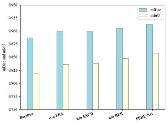
Figure 6. Ablation study results on the bladder tumor dataset BT-AMU [55].

Specifically, considering the computational complexity and efficiency of the model, we also used floating point operations (GFLOPs) and average inference time to evaluate further the impact of the three new proposed modules on the computational efficiency of the model. As shown in Table 6, the GFLOPs and inference time of “no FEA”, “no ESCD”, and “no BER” are slightly lower than those of FEBE-Net. However, the inference time of these models can meet the real-time requirements of bladder tumor segmentation tasks, and FEBE-Net has a significantly higher detection accuracy for bladder tumors. This aligns with our goal in bladder tumor segmentation tasks, which is to achieve more accurate bladder tumor segmentation while meeting real-time requirements.

Table 6. Comparison of computational efficiency results of ablation studies on the bladder tumor dataset BtAMU [55].

Models	GFLOPs (G)	Infer Time (s)
Baseline	9.74	0.0229
no FEA	20.3	0.0276
no ESCD	27.09	0.0281
no BER	18.12	0.0294
FEBE-Net	27.88	0.0318

5. Conclusions

This article proposes a new bladder tumor segmentation network based on cystoscopy images, FEBE-Net, which effectively solves the problems of the limited recovery ability of local detail features and the insufficient boundary segmentation ability of Transformer-based methods. FEBE-Net adopts the PVT v2 encoder, FEA, ESCD, and BER modules, among which the FEA module is used to mine potential local detailed feature information of bladder tumors and enhance feature representation. The ESCD module combines the fine-grained detail information captured by the FEA module in low-level features with the global semantic information in high-level features, effectively restoring the local feature details of the tumor while achieving accurate bladder tumor localization. The BER module is used to assist the decoder in more effectively preserving the boundary features of bladder tumors and refining and adjusting the final predicted feature map. Compared to the other 11 SOTA methods, the quantitative and qualitative experimental results of FEBE-Net on the bladder tumor dataset BtAMU show significant advantages, demonstrating the effectiveness and superiority of FEBE-Net in segmenting bladder tumors. In addition, the comparison of visualization results also proves that FEBE-Net can better cope with the segmentation challenges caused by size and morphology changes of bladder tumors, small bladder tumors, wrinkle background interference, and low brightness, demonstrating that FEBE-Net has strong robust stability. Meanwhile, the quantitative experimental results of FEBE-Net on five publicly available polyp datasets were significantly better than the 11 SOTA methods compared, verifying the robustness and generalization of FEBE-Net. FEBE-Net, as a computer-aided diagnostic technology, can be applied to cystoscopy image analysis tasks, reducing the dependence on visual examination by urologists and improving the accuracy of bladder tumor detection. It has important significance in clinical practice. In the future, we will establish a larger bladder tumor dataset that includes low-contrast cystoscopy images and continue to improve the model’s boundary segmentation capabilities based on this.

References

- Antoni, S.; Ferlay, J.; Soerjomataram, I.; Znaor, A.; Jemal, A.; Bray, F. Bladder Cancer Incidence and Mortality: A GlobalOverviewand Recent Trends. Eur. Urol. 2017, 71, 96–108. [Google Scholar] [CrossRef] [PubMed]
- Negassi, M.; Parupalli, U.; Suarez-Ibarrola, R.; Schmitt, A.; Hein, S.; Miernik, A.; Reiterer, A. 3D-Reconstruction and Semantic Segmentation of Cystoscopic Images. In Proceedings of the International Conference on Medical Imaging and Computer-Aided Diagnosis, MICAD 2020, Oxford, UK, 20–21 January 2020; pp. 46–55. [Google Scholar]
- Mou, L.; Zhao, Y.; Fu, H.; Liu, Y.; Cheng, J.; Zheng, Y.; Su, P.; Yang, J.; Chen, L.; Frangi, A.F.; et al. CS2-Net: Deep learning segmentation of curvilinear structures in medical imaging. Med. Image Anal. 2021, 67, 101874. [Google Scholar] [CrossRef] [PubMed]
- Xue, C.; Zhu, L.; Fu, H.; Hu, X.; Li, X.; Zhang, H.; Heng, P.-A. Global guidance network for breast lesion segmentation in ultrasound images. Med. Image Anal. 2021, 70, 101989. [Google Scholar] [CrossRef]
- Li, W.; Zeng, G.; Li, F.; Zhao, Y.; Zhang, H. FRBNet: Feedback refinement boundary network for semantic segmentation in breast ultrasound images. Biomed. Signal Process. Control 2023, 86, 105194. [Google Scholar] [CrossRef]
- Song, P.; Yang, Z.; Li, J.; Fan, H. DPCTN: Dual path context-aware transformer network for medical image segmentation. Eng. Appl. Artif. Intell. 2023, 124, 106634. [Google Scholar] [CrossRef]
- Liu, G.; Chen, Z.; Liu, D.; Chang, B.; Dou, Z. FTMF-Net: A Fourier Transform-Multiscale Feature Fusion Network for Segmentation of Small Polyp Objects. IEEE Trans. Instrum. Meas. 2023, 72, 5020815. [Google Scholar] [CrossRef]
- Zhang, R.; Lai, P.; Wan, X.; Fan, D.-J.; Gao, F.; Wu, X.-J.; Li, G. Lesion-Aware Dynamic Kernel for Polyp Segmentation. In Proceedings of the 25th International Conference on Medical Image Computing and Computer Assisted Intervention (MICCAI), Singapore, 18–22 September 2022; pp. 99–109. [Google Scholar]
- Shelhamer, E.; Long, J.; Darrell, T. Fully Convolutional Networks for Semantic Segmentation. IEEE Trans. Pattern Anal. Mach. Intell. 2017, 39, 640–651. [Google Scholar] [CrossRef]
- Ronneberger, O.; Fischer, P.; Brox, T. U-Net: Convolutional Networks for Biomedical Image Segmentation. In Proceedings of the 18th International Conference on Medical Image Computing and Computer-Assisted Intervention (MICCAI), Munich, Germany, 5–9 October 2015; pp. 234–241. [Google Scholar]
- Zhou, Z.; Siddiquee, M.M.R.; Tajbakhsh, N.; Liang, J. UNet++: A Nested U-Net Architecture for Medical Image Segmentation. In Deep Learning in Medical Image Analysis and Multimodal Learning for Clinical Decision Support, Proceedings of the 4th International Workshop, DLMIA 2018, and 8th International Workshop, ML-CDS 2018, Granada, Spain, 20 September 2018; Springer: Cham, Switzerland, 2018; Volume 11045, pp. 3–11. [Google Scholar]
- Ozan Oktay, J.S.; Folgoc, L.L.; Lee, M.; Heinrich, M.; Misawa, K.; Mori, K.; McDonagh, S.; Hammerla, N.Y.; Kainz, B.; Glocker, B.; et al. Attention U-Net: Learning Where to Look for the Pancreas. arXiv 2018, arXiv:1804.03999. [Google Scholar]
- Isensee, F.; Jaeger, P.F.; Kohl, S.A.A.; Petersen, J.; Maier-Hein, K.H. nnU-Net: A self-configuring method for deep learning-based biomedical image segmentation. Nat. Methods 2021, 18, 203. [Google Scholar] [CrossRef]
- Fan, D.-P.; Ji, G.-P.; Zhou, T.; Chen, G.; Fu, H.; Shen, J.; Shao, L. PraNet: Parallel Reverse Attention Network for Polyp Segmentation. In Proceedings of the 23rd International Conference on Medical Image Computing and Computer-Assisted Intervention, MICCAI 2020, Lima, Peru, 4–8 October 2020; pp. 263–273. [Google Scholar]
- Wei, J.; Hu, Y.; Zhang, R.; Li, Z.; Zhou, S.K.; Cui, S. Shallow Attention Network for Polyp Segmentation. In Proceedings of the 24th International Conference on Medical Image Computing and Computer Assisted Intervention, MICCAI 2021, Virtual, 27 September–1 October 2021; pp. 699–708. [Google Scholar]
- Huang, C.-H.; Wu, H.-Y.; Lin, Y.-L. HarDNet-MSEG: A simple encoder-decoder polyp segmentation neural network that achieves over 0.9 mean dice and 86 FPS. arXiv 2021, arXiv:2101.07172. [Google Scholar]
- Lou, A.; Guan, S.; Loew, M. CaraNet: Context axial reverse attention network for segmentation of small medical objects. J. Med. Imaging 2023, 10, 12032. [Google Scholar] [CrossRef] [PubMed]
- Yin, Z.; Liang, K.; Ma, Z.; Guo, J. Duplex Contextual Relation Network For Polyp Segmentation. In Proceedings of the 19th IEEE International Symposium on Biomedical Imaging, ISBI 2022, Kolkata, India, 28–31 March 2022. [Google Scholar]
- Lee, G.-E.; Cho, J.; Choi, S., II. Shallow and reverse attention network for colon polyp segmentation. Sci. Rep. 2023, 13, 15243. [Google Scholar] [CrossRef]
- Wang, X.; Girshick, R.; Gupta, A.; He, K. Non-local Neural Networks. In Proceedings of the 2018 IEEE/CVF Conference on Computer Vision and Pattern Recognition (CVPR), Salt Lake City, UT, USA, 18–23 June 2018; pp. 7794–7803. [Google Scholar]
- Schlemper, J.; Oktay, O.; Schaap, M.; Heinrich, M.; Kainz, B.; Glocker, B.; Rueckert, D. Attention gated networks: Learning to leverage salient regions in medical images. Med. Image Anal. 2019, 53, 197–207. [Google Scholar] [CrossRef] [PubMed]
- Chen, C.; Liu, X.; Ding, M.; Zheng, J.; Li, J. 3D Dilated Multi-fiber Network for Real-Time Brain Tumor Segmentation in MRI. In Proceedings of the 10th International Workshop on Machine Learning in Medical Imaging (MLMI)/22nd International Conference on Medical Image Computing and Computer-Assisted Intervention (MICCAI), Shenzhen, China, 13–17 October 2019; pp. 184–192. [Google Scholar]
- Chen, T.-W.; Wang, D.; Tao, W.; Wen, D.; Yin, L.; Ito, T.; Osa, K.; Kato, M. CASSOD-Net: Cascaded and separable structures of dilated convolution for embedded vision systems and applications. In Proceedings of the 2021 IEEE/CVF Conference on Computer Vision and Pattern Recognition Workshops, CVPRW 2021, Virtual, 19–25 June 2021; pp. 3176–3184. [Google Scholar]
- Alexey Dosovitski, L.B.; Kolesnikov, A.; Weissenborn, D.; Zhai, X.; Unterthiner, T.; Dehghani, M.; Minderer, M.; Heigold, G.; Gelly, S.; Uszkoreit, J.; et al. An Image Is Worth 16 × 16 Words: Transformers for Image Recognition at Scale. In Proceedings of the 9th International Conference on Learning Representations, ICLR 2021, Virtual, 3–7 May 2021. [Google Scholar]
- Liu, Z.; Lin, Y.; Cao, Y.; Hu, H.; Wei, Y.; Zhang, Z.; Lin, S.; Guo, B. Swin Transformer: Hierarchical Vision Transformer using Shifted Windows. In Proceedings of the 18th IEEE/CVF International Conference on Computer Vision, ICCV 2021, Virtual, 11–17 October 2021; pp. 9992–10002. [Google Scholar]
- Dong, X.; Bao, J.; Chen, D.; Zhang, W.; Yu, N.; Yuan, L.; Chen, D.; Guo, B. CSWin Transformer: A General Vision Transformer Backbone with Cross-Shaped Windows. In Proceedings of the 2022 IEEE/CVF Conference on Computer Vision and Pattern Recognition (CVPR), New Orleans, LA, USA, 18–24 June 2022; pp. 12114–12124. [Google Scholar]
- Wang, W.; Xie, E.; Li, X.; Fan, D.P.; Song, K.; Liang, D.; Lu, T.; Luo, P.; Shao, L. Pyramid Vision Transformer: A Versatile Backbone for Dense Prediction without Convolutions. In Proceedings of the 2021 IEEE/CVF International Conference on Computer Vision (ICCV), Montreal, QC, Canada, 10–17 October 2021; pp. 548–558. [Google Scholar]
- Wang, W.; Xie, E.; Li, X.; Fan, D.-P.; Song, K.; Liang, D.; Lu, T.; Luo, P.; Shao, L. PVT v2: Improved baselines with Pyramid Vision Transformer. Comput. Vis. Media 2022, 8, 415–424. [Google Scholar] [CrossRef]
- Wang, J.; Huang, Q.; Tang, F.; Meng, J.; Su, J.; Song, S. Stepwise Feature Fusion: Local Guides Global. In Proceedings of the 25th International Conference on Medical Image Computing and Computer Assisted Intervention (MICCAI), Singapore, 18–22 September 2022; pp. 110–120. [Google Scholar]
- Hatamizadeh, A.; Nath, V.; Tang, Y.; Yang, D.; Roth, H.R.; Xu, D. Swin UNETR: Swin Transformers for Semantic Segmentation of Brain Tumors in MRI Images. In Proceedings of the 7th International Brain Lesion Workshop (BrainLes), Electr Network, Virtual, 27 September 2022; pp. 272–284. [Google Scholar]
- Wu, C.; Long, C.; Li, S.; Yang, J.; Jiang, F.; Zhou, R. MSRAformer: Multiscale spatial reverse attention network for polyp segmentation. Comput. Biol. Med. 2022, 151, 106274. [Google Scholar] [CrossRef]
- Dong, B.; Wang, W.; Fan, D.-P.; Li, J.; Fu, H.; Shao, L. Polyp-PVT: Polyp Segmentation with Pyramid Vision Transformers. arXiv 2021, arXiv:2108.06932. [Google Scholar] [CrossRef]
- Tang, F.; Xu, Z.; Huang, Q.; Wang, J.; Hou, X.; Su, J.; Liu, J. DuAT: Dual-Aggregation Transformer Network for Medical Image Segmentation. In Proceedings of the 6th Chinese Conference on Pattern Recognition and Computer Vision (PRCV), Xiamen, China, 13–15 October 2024; pp. 343–356. [Google Scholar]
- Zhang, W.; Fu, C.; Zheng, Y.; Zhang, F.; Zhao, Y.; Sham, C.-W. HSNet: A hybrid semantic network for polyp segmentation. Comput. Biol. Med. 2022, 150, 106173. [Google Scholar] [CrossRef]
- Rahman, M.M.; Marculescu, R. Medical Image Segmentation via Cascaded Attention Decoding. In Proceedings of the 23rd IEEE/CVF Winter Conference on Applications of Computer Vision (WACV), Waikoloa, HI, USA, 3–7 January 2023; pp. 6211–6220. [Google Scholar]
- Yue, G.; Zhuo, G.; Yan, W.; Zhou, T.; Tang, C.; Yang, P.; Wang, T. Boundary uncertainty aware network for automated polyp segmentation. Neural Netw. 2024, 170, 390–404. [Google Scholar] [CrossRef]
- Liu, G.; Yao, S.; Liu, D.; Chang, B.; Chen, Z.; Wang, J.; Wei, J. CAFE-Net: Cross-Attention and Feature Exploration Network for polyp segmentation. Expert Syst. Appl. 2024, 238, 121754. [Google Scholar] [CrossRef]
- Liu, Y.; Yun, H.; Xia, Y.; Luan, J.; Li, M. MSGAT: Multi-scale gated axial reverse attention transformer network for medical image segmentation. Biomed. Signal Process. Control 2024, 95, 106341. [Google Scholar] [CrossRef]
- Zhang, Y.; Liu, H.; Hu, Q. TransFuse: Fusing Transformers and CNNs for Medical Image Segmentation. In Proceedings of the International Conference on Medical Image Computing and Computer Assisted Intervention (MICCAI), Electr Network, Strasbourg, France, 27 September–1 October 2021; pp. 14–24. [Google Scholar]
- Chen, J.; Lu, Y.; Yu, Q.; Luo, X.; Adeli, E.; Wang, Y.; Lu, L.; Yuille, A.L.; Zhou, Y. TransUNet: Transformers make strong encoders for medical image segmentation. arXiv 2021, arXiv:2102.04306. [Google Scholar]
- Chen, B.; Liu, Y.; Zhang, Z.; Lu, G.; Kong, A.W.K. TransAttUnet: Multi-Level Attention-Guided U-Net with Transformer for Medical Image Segmentation. IEEE Trans. Emerg. Top. Comput. 2024, 8, 55–68. [Google Scholar] [CrossRef]
- Sanderson, E.; Matuszewski, B.J. FCN-Transformer Feature Fusion for Polyp Segmentation. In Proceedings of the 26th Annual Conference on Medical Image Understanding and Analysis (MIUA), Cambridge, UK, 27–29 July 2022; pp. 892–907. [Google Scholar]
- Yuan, F.; Zhang, Z.; Fang, Z. An effective CNN and Transformer complementary network for medical image segmentation. Pattern Recognit. 2023, 136, 109228. [Google Scholar] [CrossRef]
- Song, P.; Li, J.; Fan, H.; Fan, L. TGDAUNet: Transformer and GCNN based dual-branch attention UNet for medical image segmentation. Comput. Biol. Med. 2023, 167, 107583. [Google Scholar] [CrossRef] [PubMed]
- Xu, Z.; Guo, X.; Wang, J. Enhancing skin lesion segmentation with a fusion of convolutional neural networks and transformer models. Heliyon 2024, 10, 10. [Google Scholar] [CrossRef] [PubMed]
- Zhang, W.; Lu, F.; Su, H.; Hu, Y. Dual-branch multi-information aggregation network with transformer and convolution for polyp segmentation. Comput. Biol. Med. 2024, 168, 107760. [Google Scholar] [CrossRef]
- Azad, R.; Heidari, M.; Wu, Y.; Merhof, D. Contextual Attention Network: Transformer Meets U-Net. In Proceedings of the 13th International Workshop on Machine Learning in Medical Imaging (MLMI), Singapore, 18 September 2022; pp. 377–386. [Google Scholar]
- Zhao, X.; Zhang, L.; Lu, H. Automatic Polyp Segmentation via Multi-scale Subtraction Network. In Proceedings of the International Conference on Medical Image Computing and Computer Assisted Intervention (MICCAI), Strasbourg, France, 27 September–1 October 2021; pp. 120–130. [Google Scholar]
- Duc, N.T.; Oanh, N.T.; Thuy, N.T.; Triet, T.M.; Dinh, V.S. ColonFormer: An Efficient Transformer Based Method for Colon Polyp Segmentation. IEEE Access 2022, 10, 80575–80586. [Google Scholar] [CrossRef]
- Tan-Cong, N.; Tien-Phat, N.; Gia-Han, D.; Anh-Huy, T.-D.; Nguyen, T.V.; Minh-Triet, T. CCBANet: Cascading Context and Balancing Attention for Polyp Segmentation. In Proceedings of the International Conference on Medical Image Computing and Computer Assisted Intervention (MICCAI), Strasbourg, France, 27 September–1 October 2021; pp. 633–643. [Google Scholar]
- Kim, T.; Lee, H.; Kim, D. UACANet: Uncertainty Augmented Context Attention for Polyp Segmentation. In Proceedings of the 29th ACM International Conference on Multimedia (MM), Virtual, 20–24 October 2021; pp. 2167–2175. [Google Scholar]
- Fang, Y.; Chen, C.; Yuan, Y.; Tong, K.-Y. Selective Feature Aggregation Network with Area-Boundary Constraints for Polyp Segmentation. In Proceedings of the 10th International Workshop on Machine Learning in Medical Imaging (MLMI)/22nd International Conference on Medical Image Computing and Computer-Assisted Intervention (MICCAI), Shenzhen, China, 13–17 October 2019; pp. 302–310. [Google Scholar]
- Liu, J.J.; Hou, Q.; Cheng, M.M.; Wang, C.; Feng, J. Improving Convolutional Networks With Self-Calibrated Convolutions. In Proceedings of the 2020 IEEE/CVF Conference on Computer Vision and Pattern Recognition (CVPR), Seattle, WA, USA, 13–19 June 2020; pp. 10093–10102. [Google Scholar]
- Woo, S.; Park, J.; Lee, J.-Y.; Kweon, I.S. CBAM: Convolutional Block Attention Module. In Proceedings of the 15th European Conference on Computer Vision (ECCV), Munich, Germany, 4–8 September 2018; pp. 3–19. [Google Scholar]
- Nie, C.; Xu, C.; Li, Z. MDER-Net: A Multi-Scale Detail-Enhanced Reverse Attention Network for Semantic Segmentation of Bladder Tumors in Cystoscopy Images. Mathematics 2024, 12, 1281. [Google Scholar] [CrossRef]
- Jha, D.; Smedsrud, P.H.; Riegler, M.A.; Halvorsen, P.; de Lange, T.; Johansen, D.; Johansen, H.D. Kvasir-SEG: A Segmented Polyp Dataset. In Proceedings of the 26th International Conference on MultiMedia Modeling (MMM), Daejeon, Republic of Korea, 5–8 January 2020; pp. 451–462. [Google Scholar]
- Bernal, J.; Javier Sanchez, F.; Fernandez-Esparrach, G.; Gil, D.; Rodriguez, C.; Vilarino, F. WM-DOVA maps for accurate polyp highlighting in colonoscopy: Validation vs. saliency maps from physicians. Comput. Med. Imaging Graph. 2015, 43, 99–111. [Google Scholar] [CrossRef]
- Tajbakhsh, N.; Gurudu, S.R.; Liang, J. Automated Polyp Detection in Colonoscopy Videos Using Shape and Context Information. IEEE Trans. Med. Imaging 2016, 35, 630–644. [Google Scholar] [CrossRef]
- Silva, J.; Histace, A.; Romain, O.; Dray, X.; Granado, B. Toward embedded detection of polyps in WCE images for early diagnosis of colorectal cancer. Int. J. Comput. Assist. Radiol. Surg. 2014, 9, 283–293. [Google Scholar] [CrossRef] [PubMed]
- Vazquez, D.; Bernal, J.; Javier Sanchez, F.; Fernandez-Esparrach, G.; Lopez, A.M.; Romero, A.; Drozdzal, M.; Courville, A. A Benchmark for Endoluminal Scene Segmentation of Colonoscopy Images. J. Healthc. Eng. 2017, 2017, 4037190. [Google Scholar] [CrossRef] [PubMed]
- Krizhevsky, A.; Sutskever, I.; Hinton, G.E. ImageNet Classification with Deep Convolutional Neural Networks. Commun. ACM. 2017, 60, 84–90. [Google Scholar] [CrossRef]
- Dong, Q.; Huang, D.; Xu, X.; Li, Z.; Liu, Y.; Lu, H.; Liu, Y. Content and shape attention network for bladder wall and cancer segmentation in MRIs. Comput. Biol. Med. 2022, 148, 105809. [Google Scholar] [CrossRef]
- Wang, Y.; Li, X.; Ye, X. LCANet: A Lightweight Context-Aware Network for Bladder Tumor Segmentation in MRI Images. Mathematics 2023, 11, 2357. [Google Scholar] [CrossRef]
- Li, X.; Wang, J.; Wei, H.; Cong, J.; Sun, H.; Wang, P.; Wei, B. MH2AFormer: An Efficient Multiscale Hierarchical Hybrid Attention With a Transformer for Bladder Wall and Tumor Segmentation. IEEE J. Biomed. Health Inform. 2024, 28, 4772–4784. [Google Scholar] [CrossRef] [PubMed]
- Ma, X.; Hadjiiski, L.M.; Wei, J.; Chan, H.-P.; Cha, K.H.; Cohan, R.H.; Caoili, E.M.; Samala, R.; Zhou, C.; Lu, Y. U-Net based deep learning bladder segmentation in CT urography. Med. Phys. 2019, 46, 1752–1765. [Google Scholar] [CrossRef]
- Ma, X.; Hadjiiski, L.; Wei, J.; Chan, H.-P.; Cha, K.; Cohan, R.H.; Caoili, E.M.; Samala, R.; Zhou, C.; Lu, Y. 2D and 3D Bladder Segmentation using U-Net-based Deep-Learning. In Proceedings of the Conference on Medical Imaging-Computer-Aided Diagnosis, San Diego, CA, USA, 17–20 February 2019. [Google Scholar]
- Shkolyar, E.; Jia, X.; Chang, T.C.; Trivedi, D.; Mach, K.E.; Meng, M.Q.H.; Xing, L.; Liao, J.C. Augmented Bladder Tumor Detection Using Deep Learning. Eur. Urol. 2019, 76, 714–718. [Google Scholar] [CrossRef]
- Varnyu, D.; Szirmay-Kalos, L. A Comparative Study of Deep Neural Networks for Real-Time Semantic Segmentation during the Transurethral Resection of Bladder Tumors. Diagnostics 2022, 12, 2849. [Google Scholar] [CrossRef]
- Zhang, Q.; Liang, Y.; Zhang, Y.; Tao, Z.; Li, R.; Bi, H. A comparative study of attention mechanism based deep learning methods for bladder tumor segmentation. Int. J. Med. Inform. 2023, 171, 104984. [Google Scholar] [CrossRef]
- Zhao, X.; Lai, L.; Li, Y.; Zhou, X.; Cheng, X.; Chen, Y.; Huang, H.; Guo, J.; Wang, G. A lightweight bladder tumor segmentation method based on attention mechanism. Med. Biol. Eng. Comput. 2024, 62, 1519–1534. [Google Scholar] [CrossRef] [PubMed]
- Jia, X.; Shkolyar, E.; Laurie, M.A.; Eminaga, O.; Liao, J.C.; Xing, L. Tumor detection under cystoscopy with transformer-augmented deep learning algorithm. Phys. Med. Biol. 2023, 68, 165013. [Google Scholar] [CrossRef] [PubMed]
- Bhojanapalli, S.; Chakrabarti, A.; Glasner, D.; Li, D.; Unterthiner, T.; Veit, A. Understanding Robustness of Transformers for Image Classification. In Proceedings of the 18th IEEE/CVF International Conference on Computer Vision (ICCV), Electr Network, Montreal, QC, Canada, 11–17 October 2021; pp. 10211–10221. [Google Scholar]
- Lin, Y.; Zhang, D.; Fang, X.; Chen, Y.; Cheng, K.-T.; Chen, H. Rethinking Boundary Detection in Deep Learning Models for Medical Image Segmentation. In Proceedings of the 28th International Conference on Information Processing in Medical Imaging (IPMI), San Carlos de Bariloche, Argentina, 18–23 June 2023; pp. 730–742. [Google Scholar]
- Wei, J.; Wang, S.; Huang, Q.; Assoc Advancement Artificial, I. F3Net: Fusion, Feedback and Focus for Salient Object Detection. In Proceedings of the 34th AAAI Conference on Artificial Intelligence/32nd Innovative Applications of Artificial Intelligence Conference/10th AAAI Symposium on Educational Advances in Artificial Intelligence, New York, NY, USA, 7–12 February 2020; pp. 12321–12328. [Google Scholar]
Disclaimer/Publisher’s Note: The statements, opinions and data contained in all publications are solely those of the individual author(s) and contributor(s) and not of MDPI and/or the editor(s). MDPI and/or the editor(s) disclaim responsibility for any injury to people or property resulting from any ideas, methods, instructions or products referred to in the content. |
© 2024 by the authors. Licensee MDPI, Basel, Switzerland. This article is an open access article distributed under the terms and conditions of the Creative Commons Attribution (CC BY) license (https://creativecommons.org/licenses/by/4.0/).