Optimal Epidemic Control with Nonmedical and Medical Interventions

Abstract

In this study, we investigate different epidemic control scenarios through theoretical analysis and numerical simulations. To account for two important types of control at the early ascending stage of an outbreak, nonmedical interventions, and medical treatments, a compartmental model is considered with the first control aimed at lowering the disease transmission rate through behavioral changes and the second control set to lower the period of infectiousness by means of antiviral medications and other forms of medical care. In all experiments, the implementation of control strategies reduces the daily cumulative number of cases and successfully “flattens the curve”. The reduction in the cumulative cases is achieved by eliminating or delaying new cases. This delay is incredibly valuable, as it provides public health organizations with more time to advance antiviral treatments and devise alternative preventive measures. The main theoretical result of the paper, Theorem 1, concludes that the two optimal control functions may be increasing initially. However, beyond a certain point, both controls decline (possibly causing the number of newly infected people to grow). The numerical simulations conducted by the authors confirm theoretical findings, which indicates that, ideally, around the time that early interventions become less effective, the control strategy must be upgraded through the addition of new and improved tools, such as vaccines, therapeutics, testing, air ventilation, and others, in order to successfully battle the virus going forward.

1. Introduction

Advanced modeling and parameter estimation algorithms form a solid background for the design of optimal strategies to control infectious diseases, which reduces illness and mortality rates. Vaccination, isolation, and public health education are examples of important control techniques that protect people at risk and make effective use of healthcare resources [1,2,3].

Timely control measures can mitigate the impact of outbreaks, prevent widespread transmission, and save lives. For instance, vaccination programs have been instrumental in controlling diseases such as measles, polio, and influenza [4,5]. Quarantine and isolation protocols were key in managing the spread of diseases like Ebola and COVID-19 [6]. Public health campaigns promoting handwashing and sanitation have significantly reduced the transmission of diseases such as cholera and dysentery [7,8]. The eradication of smallpox is a prime example of how global vaccination campaigns can lead to the complete elimination of a disease [9]. Similarly, the rapid response to the H1N1 influenza pandemic in 2009, including the development and distribution of vaccines, helped to control the spread of the virus and reduce its impact [10].

By analyzing data that use different models and algorithms, epidemiologists can forecast future incidence cases and evaluate various control strategies. Systematic preventive measures can help in reducing the spread of diseases. At first glance, choosing healthcare policies seems obvious, but in reality, it is a very complicated task. One needs to put forward control strategies that are practical and, at the same time, have manageable consequences. At the onset of COVID-19, lockdowns were helpful, but they were not sustainable long term [11,12,13]. Thus, choosing the best intervention at the right time is critical [14,15].

The study in [16] introduced a two-stage epidemic model for the spread of COVID-19 and proposed optimal control strategies based on actual data and cost considerations. The research underscores the importance of contact tracing and isolation in minimizing the costs and effectively curbing the spread of a disease. Numerical simulations and model analysis provide actionable recommendations for public health authorities, highlighting the critical role of controlling the transmission rate in epidemic management.

The research in [17] modeled the spread of COVID-19 and assessed the impact of social intervention measures during the early outbreak phase, focusing on optimal control strategies and the identifiability of model parameters. It found that optimal control strategies, especially social distancing and self-isolation, as well as significantly reduced transmission rates when implemented early. The study emphasized the importance of structural identifiability for accurate parameter estimation in COVID-19 models. It shows that implementing control measures effectively “flattens the curve” and lowers the burden on healthcare systems.

Another study, [18], focused on an $SIR$ model with saturated incidence and treatment rates, analyzing equilibrium points, bifurcation, and optimal control strategies that utilize vaccination and treatment as well as antiviral medication, in order to contain the outbreak. The authors’ findings, derived from numerical simulations and efficiency analysis, demonstrated that vaccination control stands to reduce the cumulative number of infections more rapidly than control by antiviral treatment. This research underscores the value of mathematical modeling in epidemiology and the strategic implementation of vaccination to prevent disease transmission.

2. Control of an Emerging Disease

In the study of epidemic control, the effective management of disease spread is crucial, particularly at the onset of an outbreak. While the importance of vaccination in fighting infectious diseases is undeniable, it takes time to develop a vaccine for an emerging strain. Various parameters, including environmental factors, immunity patterns, and behavioral changes, impact the circulation of a virus. Social distancing and personal hygiene measures (non-medical interventions) play an important role in containing the disease at an early ascending stage. By optimizing the implementation of non-medical interventions over time, the effectiveness of these interventions can be increased.

Another essential component of control and prevention is treatment with antiviral medications, which makes it possible to reduce the period of infectiousness and/or reduce the disease fatality rate. To account for these two important types of control, we consider the following $SIR$ (Susceptible-Infectious-Removed) model [19] for early disease transmission:

$$\begin{array}{l}{\displaystyle \frac{d\mathcal{S}}{dt}}=-\beta {\displaystyle \frac{\mathcal{S}\left(t\right)\mathcal{I}\left(t\right)}{N}}\\ {\displaystyle \frac{d\mathcal{I}}{dt}}=\beta {\displaystyle \frac{\mathcal{S}\left(t\right)\mathcal{I}\left(t\right)}{N}}-\gamma \mathcal{I}\left(t\right)\\ {\displaystyle \frac{d\mathcal{R}}{dt}}=\gamma \mathcal{I}\left(t\right)\end{array}$$

(1)

In this system (1), we assume that recovered individuals gain immunity for the duration of the study period and do not return to the susceptible class $\mathcal{S}$. Additionally, we assume that the natural birth and death rates balance one another, and the number of deaths due to the disease is expected to be negligible relative to the total population, N, so that the removed class, $\mathcal{R}$, is mostly comprised of recovered individuals. Therefore, the removed class, $\mathcal{R}$, is essentially viewed as recovered, and the two disease parameters $\beta >0$ and $\gamma >0$ are the transmission and recovery rates, respectively. Individuals leave the infectious class, $\mathcal{I}$, after being infected for an average time period $1/\gamma$.

The focus of this research regards introducing optimal controls during the initial weeks of a pandemic in order to delay and reduce the daily number of infections [20]. This approach enables health centers and decision-making organizations to implement more effective operations. In what follows, we incorporate two different kinds of control in the $SIR$ model [21], resulting in the system ${\displaystyle \frac{d\mathbf{x}}{dt}}=f(\mathbf{x},\mathbf{u})$, where

$$\begin{array}{l}{f}_1(\mathbf{x},\mathbf{u}):=-\beta (1-u_1\left(t\right))S\left(t\right)I\left(t\right)\\ f_2(\mathbf{x},\mathbf{u}):=\beta (1-u_1\left(t\right))S\left(t\right)I\left(t\right)-(\gamma +\epsilon u_2\left(t\right))I\left(t\right)\\ f_3(\mathbf{x},\mathbf{u}):=(\gamma +\epsilon u_2\left(t\right))I\left(t\right).\end{array}$$

(2)

Here, $S\left(t\right):={\displaystyle \frac{\mathcal{S}\left(t\right)}{N}}$, $I\left(t\right):={\displaystyle \frac{\mathcal{I}\left(t\right)}{N}}$, and $R\left(t\right):={\displaystyle \frac{\mathcal{R}\left(t\right)}{N}}$ are the normalized susceptible, infected, and removed compartments, respectively; N is the population of the region at the beginning of the study period. The function $u_1\left(t\right)$ represents nonmedical controls (social distancing, remote work, online education, restriction on travel, lockdowns, etc.), while $u_2\left(t\right)$ stands for treatment with antiviral medications and other medical interventions. A positive parameter, $\epsilon$, is the efficacy of antiviral treatments [22]. In the above, $\mathbf{x}:={[S,I,R]}^{\top }$, $\mathbf{u}:={[u_1,u_2]}^{\top }$, and the admissible set for each control function is

$$\begin{array}{c}\mathcal{U}=\left\{u_i\in {\mathcal{L}}^1[0,T],0\le u_i\left(t\right)<1,i=1,2\right\}.\end{array}$$

(3)

In (2), the first control, $u_1\left(t\right)$, aims to change the disease transmission rate from $\beta$ to $\beta (1-u_1\left(t\right))$, while the second control, $u_2\left(t\right)$, is expected to reduce the period of infectiousness, which is ${\displaystyle \frac{1}{\gamma }}$ in the initial system (1). In combination, the two controls, $u_1\left(t\right)$ and $u_2\left(t\right)$, are meant to minimize the force of infection, $\beta (1-u_1\left(t\right))S\left(t\right)I\left(t\right)$, while keeping the costs at bay. The costs are considered in a general sense, which includes a negative impact on mental health, education, the economy, and on the overall quality of life.

In Lemma 1 below, we show that, following the introduction of a time-dependent transmission rate, $\beta \left(t\right):=\beta (1-u_1\left(t\right))$, and a time-dependent recovery rate, $\gamma \left(t\right):=\gamma +\epsilon u_2\left(t\right)$, the model ${\displaystyle \frac{d\mathbf{x}}{dt}}=f(\mathbf{x},u)$ in (2) remains well-defined in the sense that the state variables $S\left(t\right),I\left(t\right),R\left(t\right),$ originating in a positive octant do not leave the octant for all values of $t>0$. The proof of this lemma is similar to the argument in [23], where the system (2) was considered with non-medical controls only (that is, $u_2\left(t\right)=0$).

Lemma 1

([23]). Let $u_i\left(t\right),$$i=1,2$ be admissible control trajectories with $\mathbf{x}\left(t\right)$, satisfying ${\displaystyle \frac{d\mathbf{x}}{dt}}=f(\mathbf{x},\mathbf{u})$ given by (2) and

$$(S\left(0\right),I\left(0\right),R\left(0\right))\in {\Delta }^2:=\{(z_1,z_2,z_3)\in {\mathbb{R}}^3:z_1+z_2+z_3=1,z_1,z_2,z_3\ge 0\},$$

where the probability simplex is ${\mathbb{R}}^3$. Then, $(S\left(t\right),I\left(t\right),R\left(t\right))\in {\Delta }^2$ for all $t\ge 0$.

Note that the argument in [23] implies that the conclusion of Lemma 1 is not limited to $\beta \left(t\right):=\beta (1-u_1\left(t\right))$ and $\gamma \left(t\right):=\gamma +\epsilon u_2\left(t\right)$. It is valid for any integrable non-negative functions $\beta \left(t\right)$ and $\gamma \left(t\right)$. To optimize the implementation of both controls, $u_1\left(t\right)$ and $u_2\left(t\right)$, we consider the following objective functional:

$$\begin{array}{cc}J(\mathbf{x},\mathbf{u}):& ={\int }_0^T\left\{(\beta (1-u_1\left(t\right))S\left(t\right)I\left(t\right)+{\lambda }^{\top }C\left(\mathbf{u}\left(t\right)\right)\right\}dt.\end{array}$$

According to system (2), one can integrate the first term to obtain

$$\begin{array}{cc}J(\mathbf{x},\mathbf{u})& =S\left(0\right)-S\left(T\right)+{\int }_0^T{\lambda }^{\top }C\left(\mathbf{u}\left(t\right)\right)dt:=h\left(\mathbf{x}\left(T\right)\right)+{\int }_0^{T}L(\mathbf{x}\left(t\right),\mathbf{u}\left(t\right))dt,\end{array}$$

(4)

where $C\left(\mathbf{u}\right):={[C_1\left(u_1\right),C_2\left(u_2\right)]}^{\top }$ is the assumed cost of control and $\lambda :={[{\lambda }_1,{\lambda }_2]}^{\top }$, ${\lambda }_1,{\lambda }_2>0$, is the regularization parameter (weight). As our numerical experiments show, the choice of the cost function, $C\left(\mathbf{u}\right)$, significantly influences the resulting control strategy. From a practical standpoint, neither $u_1\left(t\right)$ nor $u_2\left(t\right)$ should take negative values. At the same time, the cost, $C_i\left(u_i\right)$, must increase dramatically as $u_i\left(t\right)$ approaches 1, which is the upper bound of the feasible set (3), since it is impossible to entirely eliminate the disease transmission $(u_1\left(t\right)=1)$. It is equally impossible to reach the full capacity of antiviral treatment ($u_2\left(t\right)=1$) due to the limitations of testing and other factors. Therefore, in our approach, we impose the following assumptions on the cost functions $C_1\left(u_1\right)$ and $C_2\left(u_2\right)$ [23]:

$$\begin{array}{c}{C}_i^{″}\left(u\right)>0,{\mathit{C}}_i\left(0\right)=0,C_i^{\prime }\left(u\right)>0\mathrm{for}u>0,\\ C_i^{\prime }\left(u\right)<0\mathrm{for}u<0\mathrm{and}\underset{u\to 1^{-}}{lim}{C}_i\left(u\right)=\infty ,i=1,2.\end{array}$$

(5)

These assumptions on the cost of control were first proposed in [23] for a special case when $u_2\left(t\right)=0$. The authors of [23] employed the techniques of machine learning to show that under assumptions (5), the global minimum of the Hamiltonian gives rise to the optimal control strategy, $u_1\left(t\right)$, which stays within the feasible set (3) for all values of $t\in [0,T]$. Assumptions (5) are the alternative to a more traditional cost function, $C\left(u\right)=u^2$, that is often used in the control literature. However, $C\left(u\right)=u^2$ does not generally prevent the global minimum from becoming greater than 1 for some values of t, even for large weights $\lambda .$

3. Theoretical Study and Discussion

In this section, we state and prove our main theoretical result.

Theorem 1.

Let $u\in \mathcal{U}$ be an optimal control strategy with respect to the objective functional $J(\mathbf{x},\mathbf{u})$ defined in (4) and biological model $\dot{\mathbf{x}}=f(\mathbf{x},\mathbf{u})$, $\mathbf{x}\left(0\right)={\mathbf{x}}_{\mathbf{0}}$, introduced in (2), with $C\left(\mathbf{u}\right):={[C_1\left(u_1\right),C_2\left(u_2\right)]}^{\top }$ satisfying (5) and $\lambda :={[{\lambda }_1,{\lambda }_2]}^{\top }$, ${\lambda }_1,{\lambda }_2>0$. Then, there is $\tau \in [0,T)$ such that for any $t\in (\tau ,T)$, the derivative, ${\displaystyle \frac{d{u}_i}{dt}}$, $i=1,2,$ exists, and ${\displaystyle \frac{d{u}_i}{dt}}<0$. In other words, there is $\tau \in [0,T)$ such that for any $t\in (\tau ,T)$, both optimal controls, $u_1\left(t\right)$ and $u_2\left(t\right)$, are decreasing.

Proof. 

According to the Pontryagin’s Minimum Principle [24,25], if $u\in \mathcal{U}$ is an optimal control with respect to the objective functional $J(\mathbf{x},\mathbf{u})=h\left(\mathbf{x}\left(T\right)\right)+{\int }_0^{T}L(\mathbf{x}\left(t\right),\mathbf{u}\left(t\right))dt$ and the system $\dot{\mathbf{x}}=f(\mathbf{x},\mathbf{u})$, $\mathbf{x}\left(0\right)={\mathbf{x}}_{\mathbf{0}}$, then there is a trajectory $\mathbf{p}\left(t\right)$ such that

$$\dot{\mathbf{p}}\left(t\right)={\left.-{{\partial }_{\mathbf{x}}H(\mathbf{x},\mathbf{u},\mathbf{p})}^{\top }\right|}_{\mathbf{x}\left(t\right),\mathbf{u}\left(t\right),\mathbf{p}\left(t\right)},\mathbf{p}\left(T\right)={\left.{\partial }_{\mathbf{x}}h{\left(\mathbf{x}\right)}^{\top }\right|}_{\mathbf{x}\left(T\right)},$$

(6)

$$\mathbf{u}\left(t\right)=\underset{\mathbf{v}\in \mathcal{U}}{arg\; min}H(\mathbf{x}\left(t\right),\mathbf{v}\left(t\right),\mathbf{p}\left(t\right)),H(\mathbf{x},\mathbf{v},\mathbf{p}):=L(\mathbf{x},\mathbf{v})+{\mathbf{p}}^{\top }f(\mathbf{x},\mathbf{v}).$$

(7)

By the properties (5) of the cost, $C\left(\mathbf{u}\right)$, one has $C_i^{\prime }\left(u\right)>0$ for $u>0$ and ${lim}_{u\to 1^{-}}{C}_i\left(u\right)=\infty$, which prevent any $\mathbf{u}={[u_1,u_2]}^{\top }$, $u_i\ge 1$, $i=1,2,$ from being the optimal of $H(\mathbf{x},\mathbf{u},\mathbf{p})$ with respect to $\mathbf{u}$ at any time $t\in [0,T]$. Therefore, the Karush–Kuhn–Tucker (KKT) conditions for the optimal control problem (2)–(4) take the form

$$\begin{array}{cc}& {\partial }_{\mathbf{u}}H(\mathbf{x},\mathbf{u},\mathbf{p})-q\left(t\right)=\mathbf{0},q\left(t\right):={[q_1\left(t\right),q_2\left(t\right)]}^{\top }\end{array}$$

(K1)

$$\begin{array}{cc}& \dot{\mathbf{p}}\left(t\right)={\left.-{{\partial }_{\mathbf{x}}H(\mathbf{x},\mathbf{u},\mathbf{p})}^{\top }\right|}_{\mathbf{x}\left(t\right),\mathbf{u}\left(t\right),\mathbf{p}\left(t\right)},\mathbf{p}\left(T\right)={\left.{\partial }_{\mathbf{x}}h{\left(\mathbf{x}\right)}^{\top }\right|}_{\mathbf{x}\left(T\right)}\end{array}$$

(K2)

$$\begin{array}{cc}& \dot{\mathbf{x}}\left(t\right)=f(\mathbf{x},\mathbf{u}),\mathbf{x}\left(0\right)={\mathbf{x}}_0\end{array}$$

(K3)

$$\begin{array}{cc}& q_i\left(t\right)\ge 0,u_i\left(t\right)\ge 0,i=1,2,q{\left(t\right)}^{\top }\mathbf{u}\left(t\right)=0\forall t\in [0,T].\end{array}$$

(K4)

As it follows from (2), (4) and (7),

$$\begin{array}{ll}{\partial }_{\mathbf{u}}H(\mathbf{x},\mathbf{u},\mathbf{p})& ={\partial }_{\mathbf{u}}L(\mathbf{x},\mathbf{u})+{\mathbf{p}}^{\top }{\partial }_{\mathbf{u}}f(\mathbf{x},\mathbf{u})\\ & =\left[\begin{array}{cc}{\displaystyle \frac{\partial L}{\partial u_1}}& {\displaystyle \frac{\partial L}{\partial u_2}}\end{array}\right]+[p_1,p_2,p_3]\left[\begin{array}{cc}{\displaystyle \frac{\partial f_1}{\partial u_1}}& {\displaystyle \frac{\partial f_1}{\partial u_2}}\\ {\displaystyle \frac{\partial f_2}{\partial u_1}}& {\displaystyle \frac{\partial f_2}{\partial u_2}}\\ {\displaystyle \frac{\partial f_3}{\partial u_1}}& {\displaystyle \frac{\partial f_3}{\partial u_2}}\end{array}\right]\\ & =\left[\begin{array}{cc}{\lambda }_1{\displaystyle \frac{d{c}_1}{d{u}_1}}& {\lambda }_2{\displaystyle \frac{d{c}_2}{d{u}_2}}\end{array}\right]+[p_1,p_2,p_3]\left[\begin{array}{cc}\beta SI& 0\\ -\beta SI& -\epsilon I\\ 0& \epsilon I\end{array}\right],\end{array}$$

(8)

which yields

$$\begin{array}{cc}{\lambda }_1{\displaystyle \frac{d{c}_1}{d{u}_1}}-q_1\left(t\right)& =-\beta (p_1-p_2)SI\end{array}$$

(9)

$$\begin{array}{cc}{\lambda }_2{\displaystyle \frac{d{c}_2}{d{u}_2}}-q_2\left(t\right)& =-\epsilon (p_3-p_2)I.\end{array}$$

(10)

To show that on some $(\tau ,T)$ the derivative ${\displaystyle \frac{d{u}_1}{dt}}$ exists that and ${\displaystyle \frac{d{u}_1}{dt}}<0$, we follow [23]. Conditions (K2) and (K3) imply that $(p_1-p_2)SI$ is differentiable and therefore continuous for any $t\in [0,T]$. From Lemma 1, one concludes that $S\left(t\right),I\left(t\right)>0$ as long as $S\left(0\right)$ and $I\left(0\right)$ are positive. On the other hand, since $p_1\left(T\right)=-1<0=p_2\left(T\right)$, there is ${\tau }_1\in [0,T)$ such that $p_1\left(t\right)-p_2\left(t\right)<0$ for all $t\in [{\tau }_1,T)$. Suppose at some point $t\in [{\tau }_1,T]$, where the Lagrange multiplier, $q_1\left(t\right)$, is greater than zero. Then from (K4), it follows that $u_1\left(t\right)=0$. By (5), this implies that ${\displaystyle \frac{d{c}_1}{d{u}_1}}\left(t\right)=0$, which means that in (9) ${\displaystyle \frac{d{c}_1}{d{u}_1}}\left(t\right)-q_1\left(t\right)<0$, while $-\beta (p_1-p_2)SI>0$. Hence, we arrive at the contradiction. Therefore, for any $t\in [{\tau }_1,T]$, one has $q_1\left(t\right)=0$ and ${\lambda }_1{\displaystyle \frac{d{c}_1}{d{u}_1}}=-\beta (p_1-p_2)SI$. By the implicit function theorem, for $t\in ({\tau }_1,T)$ the derivative ${\displaystyle \frac{d{u}_1}{dt}}$ exists, and

$$\begin{array}{c}{\displaystyle \frac{d{u}_1}{dt}}=-{\displaystyle \frac{\beta {\left[S\left(t\right)I\left(t\right)(p_1\left(t\right)-p_2\left(t\right))\right]}^{\prime }}{{\lambda }_1{c}_1^{\prime \prime }\left(u_1\right)}}\mathrm{for} \mathrm{all}t\in ({\tau }_1,T).\end{array}$$

(11)

Taking into consideration (2), (4), and (7), one obtains

$$\begin{array}{ll}{\partial }_{\mathbf{x}}H(\mathbf{x},\mathbf{u},\mathbf{p})& ={\partial }_{\mathbf{x}}L(\mathbf{x},\mathbf{u})+{\mathbf{p}}^{\top }{\partial }_{\mathbf{x}}f(\mathbf{x},\mathbf{u})\\ & =\left[\begin{array}{ccc}{\displaystyle \frac{\partial L}{\partial S}}& {\displaystyle \frac{\partial L}{\partial I}}& {\displaystyle \frac{\partial L}{\partial R}}\end{array}\right]+[p_1,p_2,p_3]\left[\begin{array}{ccc}{\displaystyle \frac{\partial f_1}{\partial S}}& {\displaystyle \frac{\partial f_1}{\partial I}}& {\displaystyle \frac{\partial f_1}{\partial R}}\\ {\displaystyle \frac{\partial f_2}{\partial S}}& {\displaystyle \frac{\partial f_2}{\partial I}}& {\displaystyle \frac{\partial f_2}{\partial R}}\\ {\displaystyle \frac{\partial f_3}{\partial S}}& {\displaystyle \frac{\partial f_3}{\partial I}}& {\displaystyle \frac{\partial f_3}{\partial R}}\end{array}\right]\\ & =\left[\begin{array}{ccc}0& 0& 0\end{array}\right]+[p_1,p_2,p_3]\left[\begin{array}{ccc}-\beta (1-u_1)I& -\beta (1-u_1)S& 0\\ \beta (1-u_1)I& \beta (1-u_1)S-(\gamma +\epsilon u_2)& 0\\ 0& (\gamma +\epsilon u_2)& 0\end{array}\right].\end{array}$$

(12)

Furthermore, from (4) one obtains ${\partial }_{x}h\left(\mathbf{x}\right)={[-1,0,0]}^{\top }$. This, together with (12), implies that $p_3\left(t\right)=0$, and the costate equations for $p_1\left(t\right)$ and $p_2\left(t\right)$ take the following form:

$$\begin{array}{ll}{\dot{p}}_1=& \beta (1-u_1\left(t\right))(p_1\left(t\right)-p_2\left(t\right))I\left(t\right)\\ {\dot{p}}_2=& \beta (1-u_1\left(t\right))(p_1\left(t\right)-p_2\left(t\right))S\left(t\right)+p_2\left(t\right)(\gamma +\epsilon u_2\left(t\right))\\ & p_1\left(T\right)=-1,p_2\left(T\right)=0.\end{array}$$

(13)

Combining (2) and (13), one can rewrite ${\left[S\left(t\right)I\left(t\right)(p_1\left(t\right)-p_2\left(t\right))\right]}^{\prime }$ as follows:

$$\begin{array}{ll}{\left[S\left(t\right)I\left(t\right)(p_1\left(t\right)-p_2\left(t\right))\right]}^{\prime }& =(S^{\prime }I+S{I}^{\prime })(p_1-p_2)+(p_1^{\prime }-p_2^{\prime })S\left(t\right)I\left(t\right)\\ & =\left\{-\beta (1-u_1)S{I}^2+\beta (1-u_1)S^{2}I-(\gamma +\epsilon u_2)SI\right\}(p_1-p_2)\\ & +\left\{\beta (p_1-p_2)(1-u_1)(I-S)-p_2(\gamma +\epsilon u_2)\right\}SI\\ & =-p_1(\gamma +\epsilon u_2)SI.\end{array}$$

(14)

From (14) and (11), one concludes

$$\begin{array}{c}{\displaystyle \frac{d{u}_1}{dt}}={\displaystyle \frac{\beta p_1(\gamma +\epsilon u_2)SI}{{\lambda }_1{c}_1^{\prime \prime }\left(u_1\right)}}\mathrm{for} \mathrm{all}t\in ({\tau }_1,T).\end{array}$$

(15)

Since $p_1\left(T\right)=-1<0$ and $S\left(t\right),I\left(t\right)>0$, while $\gamma +\epsilon u_2>0$, ${\lambda }_1{c}_1^{″}\left(u_1\right)>0$ for $t\in [0,T]$, there exists ${\tau }_2\in [0,T)$ such that $p_1\left(t\right)<0$ and ${\displaystyle \frac{\beta p_1(\gamma +\epsilon u_2)SI}{{\lambda }_1{c}_1^{″}\left(u_1\right)}}<0$ for all $t\in [{\tau }_2,T]$. Let $\tau =max({\tau }_1,{\tau }_2)$; then, ${\displaystyle \frac{d{u}_1}{dt}}$ is negative in $(\tau ,T).$ As noted above, $p_3\left(t\right)=0$; therefore, identity (10) yields

$$\begin{array}{cc}{\lambda }_2{\displaystyle \frac{d{c}_2}{d{u}_2}}-q_2\left(t\right)& =\epsilon p_{2}I.\end{array}$$

(16)

Taking into account (13), one arrives at

$${\displaystyle \frac{d}{dt}}\left(p_2\left(t\right)e^{{\int }_t^T(\gamma +\epsilon u_2\left(\mu \right))d\mu }\right)=\beta (1-u_1\left(t\right))(p_1\left(t\right)-p_2\left(t\right))S\left(t\right)e^{{\int }_t^T(\gamma +\epsilon u_2\left(\mu \right))d\mu }.$$

(17)

Integrating (17) from t to T and substituting $p\left(T\right)=0$, one obtains

$$p_2\left(t\right)=-\beta e^{-{\int }_t^T(\gamma +\epsilon u_2\left(\mu \right))d\mu }{\int }_t^T(1-u_1\left(\nu \right))(p_1\left(\nu \right)-p_2\left(\nu \right))S\left(\nu \right)e^{{\int }_{\nu }^T(\gamma +\epsilon u_2\left(\mu \right))d\mu }d\nu .$$

(18)

As shown above, $p_1\left(t\right)-p_2\left(t\right)$ is negative on $[\tau ,T]$. Thus, (3) and (18) imply that $p_2\left(t\right)>0$ for all $t\in [\tau ,T)$. Using the same argument as in the case of $u_1\left(t\right)$, one can now conclude that $q_2\left(t\right)$ in (16) is equal to zero on $[\tau ,T]$, that is, the constraint $u_2\left(t\right)\ge 0$ is not active for $t\in [\tau ,T)$, and ${\lambda }_2{\displaystyle \frac{d{c}_2}{d{u}_2}}=\epsilon p_{2}I$. By the implicit function theorem, for $t\in (\tau ,T)$, the derivative ${\displaystyle \frac{d{u}_2}{dt}}$ exists, and

$$\begin{array}{c}{\displaystyle \frac{d{u}_2}{dt}}={\displaystyle \frac{\epsilon {\left[p_{2}I\right]}^{\prime }}{{\lambda }_2{c}_2^{″}\left(u_2\right)}}\mathrm{for} \mathrm{all}t\in (\tau ,T).\end{array}$$

(19)

From (2) and (13), one has

$$\begin{array}{ll}{\left[p_{2}I\right]}^{\prime }& =\left\{\beta (1-u_1)(p_1-p_2)S+p_2(\gamma +\epsilon u_2)\right\}I+p_2\left\{\beta (1-u_1)SI-(\gamma +\epsilon u_2)I\right\}\\ & =\beta p_1(1-u_1)SI<0\mathrm{on}[\tau ,T],\end{array}$$

since $p_1\left(t\right)<0$ for all $t\in [{\tau }_2,T]$ and $\tau \ge {\tau }_2$. This implies that ${\displaystyle \frac{d{u}_2}{dt}}<0$ in $(\tau ,T)$, which completes the proof. □

Remark 1.

According to (4), (5), and (7), ${\partial }_{\mathbf{u}}^{2}H(\mathbf{x},\mathbf{u},\mathbf{p})=\left[\begin{array}{cc}{\lambda }_1{c}_1^{″}\left(u_1\right)& 0\\ 0& {\lambda }_2{c}_2^{″}\left(u_2\right)\end{array}\right]$. Therefore, ${\partial }_{\mathbf{u}}^{2}H(\mathbf{x},\mathbf{u},\mathbf{p})$ is positive definite, and $H(\mathbf{x},\mathbf{u},\mathbf{p})$ has a unique global minimum with respect to $\mathbf{u}$. From the proof of Theorem 1, it follows that both coordinates of the global minimum, $u_1\left(t\right)$ and $u_2\left(t\right)$, are guaranteed to be less than 1 pointwisely, but they are not guaranteed to be greater than 0 necessarily, which means that the solution to our optimal control problem can be a local minimum rather than global. The reason that the coordinates of the global minimum, $u_i\left(t\right)$, $i=1,2$, can potentially be less than zero for some values of t is that, counterintuitively, a smaller effective reproduction number, $r\left(t\right)$, in the SIR model does not always imply a smaller cumulative number of infected people: $S\left(0\right)-S\left(t\right)$. Hence, even though for system (2), the effective reproduction number, $r\left(t\right)=\beta (1-u_1\left(t\right))/(\gamma +\epsilon u_2\left(t\right))$, goes down with more control, it does not guarantee that $r\left(t\right)\ge \overline{r}\left(t\right)$ yields $S\left(t\right)\le \overline{S}\left(t\right)$ for every value of t. One can, however, show that if $r\left(t\right)\ge \overline{r}\left(t\right)$ and $r\left(t\right)$ is non-increasing, then $S\left(t\right)\le \overline{S}\left(t\right)$. This result is important in its own right. Its proof is given in Appendix A.

Remark 2.

Despite the fact that, theoretically, the solution to our optimal control problem can be a local minimum rather than global, in all numerical experiments presented in the next section, the optimal strategy is a unique global minimum. In other words, in all our experiments, the optimal control has been computed from the first-order necessary condition for unconstrained minimization, and non-negativity constraints have held without being enforced. For all cost functions, $C\left(\mathbf{u}\right(t\left)\right)$, satisfying (5), the global minimum of $H(\mathbf{x},\mathbf{u},\mathbf{p})$ with respect to $\mathbf{u}$ has non-negative coordinates $u_i\left(t\right)$, $i=1,2$. That is, $\mathbf{u}\left(t\right)={arg\; min}_{\mathbf{v}\in \mathcal{U}}H(\mathbf{x}\left(t\right),\mathbf{v}\left(t\right),\mathbf{p}\left(t\right))$ is equivalent to $\mathbf{u}\left(t\right)={arg\; min}_{\mathbf{v}\in {\mathcal{L}}^1[0,T]}H(\mathbf{x}\left(t\right),\mathbf{v}\left(t\right),\mathbf{p}\left(t\right))$ for all $t\in [0,T].$ This illustrates that conditions (5) lead to a practically justified mitigation scenario. Numerical simulations have also confirmed, as proven in Theorem 1, that both controls, $u_1\left(t\right)$ and $u_2\left(t\right)$, were decreasing toward the end of the study period.

4. Numerical Experiments

In our numerical study, we used a second-order trust region algorithm for non-linear optimization ‘lsqnonlin’ combined with the ode15s built-in function to approximate the solution to an optimal control problem (4) subject to a compartmental model (2) and costate system (13). For every value of ${\mathbf{u}}_k$, we solved system (2) forward in time (starting with $\mathbf{x}\left(0\right)={\mathbf{x}}_{\mathbf{0}}$), to obtain ${\mathbf{x}}_k$ using ode15s. Then, system (13) was solved back in time using ode15s to obtain ${\mathbf{p}}_k$. Given $({\mathbf{x}}_k,{\mathbf{u}}_k,{\mathbf{p}}_k)$, we found ${\mathbf{u}}_{k+1}$ by applying the second-order trust region ‘lsqnonlin’ algorithm.

Following [23], we consider three different cost functions, $C_{i,1}$, $C_{i,2}$, and $C_{i,3},$ satisfying conditions (5):

$$\begin{array}{rr}{C}_{i,1}\left(u\right)=-0.830071ln(1-u^2),& C_{i,2}\left(u\right)=-0.672850uln(1-u)\hfill \\ C_{i,3}\left(u\right)=-u-ln(1-u),& C_{i,4}\left(u\right)=1.424546u^{2}i=1,2.\hfill \end{array}$$

(20)

In (20), the coefficients have been chosen to minimize the weighted distance [23]:

$$\begin{array}{c}{\int }_0^{1}w\left(z\right){|C_{i,j}\left(z\right)-C_{i,3}\left(z\right)|}^{2}dz,w\left(z\right)=\sqrt{1-z^2},j=1,2,4.\end{array}$$

(21)

The cost of control, $C_{i,1}\left(u\right)$, $C_{i,2}\left(u\right)$, and $C_{i,3}\left(u\right)$, is infinite as u approaches its ultimate value 1. For comparison, we also used the cost function $C_{i,4}\left(u\right)=u^2$, for which (5) does not hold. The cost function $C_{i,4}\left(u\right)=u^2$ is popular in applications of control theory in epidemiology and other fields, since for this function the first-order optimality condition is linear with respect to u. This is a useful property that simplifies numerical algorithms. However, the cost of control, $C_{i,4}\left(u\right)$, is finite at $u=1$, which is not realistic in real-world scenarios. Figures 4, 7 and 12 show that the global minimum, $\mathbf{u}\left(t\right)$, of the Hamiltonian, $H\left(\mathbf{x}\right(t),\mathbf{u}(t),\mathbf{p}(t\left)\right)$, did not stay in the range of $[0,1]$ when the cost was given by $C_{i,4}\left(u\right)=u^2$, especially for small values of ${\lambda }_i$, $i=1,2$. Thus, an explicit constraint $u_i\left(t\right)\le 1$ must be imposed in the case of $C_{i,4}\left(u\right)$. Even with the constraint $u_i\left(t\right)\le 1$, the optimal control function, $\mathbf{u}\left(t\right)$, often reaches the ultimate level [17], $u_i\left(t\right)=1$, which is not practical.

In all numerical experiments presented in this section, $C_{1,j}\left(u\right)=C_{2,j}\left(u\right)$, $j=1,2,3,4$. Therefore, moving forward, we omitted the first index and set $C_{i,j}\left(u\right):=C_j\left(u\right)$. A comparison of the four cost functions in the interval $[-1,1]$ is illustrated in Figure 1.

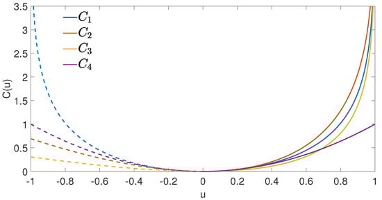
Figure 1. Comparison of the four control cost functions used in numerical experiments below: $C_1\left(u\right)=-0.830071ln(1-u^2),$ $C_2\left(u\right)=-0.672850uln(1-u)$, $C_3\left(u\right)=-u-ln(1-u)$, $C_4\left(u\right)=1.424546u^2$.

In this study, numerical simulations were conducted for ${\lambda }_1$ and ${\lambda }_2$ equal to $0.1$, $0.05$, $0.01$, $0.001$, and ${10}^{-7}$. Three different scenarios have been explored. First, there is only non-medical control, $u_1\left(t\right)$, (social distancing, behavioral changes, hand washing, etc.) in the system, and treatment with antiviral medications, $u_2\left(t\right)$, is not available. Second, only control $u_2\left(t\right)$, treatment with antiviral medications is applied; there is no social distancing. And third, controls $u_1\left(t\right)$ and $u_2\left(t\right)$, medical and non-medical are used in combination. In our experiments, the population of the region, N, was assumed to be ${10}^7$. The initial number of infected individuals on day 1 was 200, and the duration of the study period was 120 days. The transmission rate, $\beta$, and recovery rate, $\gamma$, were assumed to be $0.3$ and $0.1$, respectively, leading to the basic reproduction number $r=3$. The efficacy of antiviral medication, $\epsilon$, was assumed to be $0.5$ when applicable.

4.1. Scenario 1: Social Distancing Control Only

In the first scenario, only one (non-medical) control, $u_1\left(t\right)$, was applied (Figure 2, Figure 3 and Figure 4). As one can see in the figures, when the weight of control ${\lambda }_1$ was increased, the effectiveness of the control went down; see also Table 1 that illustrates how $\mathcal{I}\left(t\right)$ changes over time for the cost $C_1\left(u\right)$ with different values of ${\lambda }_1$ (find similar Table A13, Table A14 and Table A15 for $C_2$, $C_3$, and $C_4$ in the Appendix A). One can conclude from Figure 2 that control $u_1\left(t\right)$ works by eliminating some cases but also by delaying some of them. Therefore, even though the cumulative number of infections in the controlled environment was significantly less than in the environment with no control, toward the end of the study period, the daily number of infected individuals in the controlled environment may end up being higher.

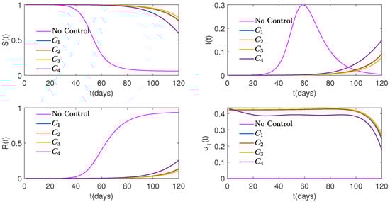
Figure 2. Graphs of Susceptible $S\left(t\right)$ (top on the left), Infected $I\left(t\right)$ (top on the right), and Recovered $R\left(t\right)$ (bottom on the left) people, as well as control $u_1\left(t\right)$ (bottom on the right) over time for four different cost functions $C_1,C_2,C_3,C_4$ versus No Control when weight is ${\lambda }_1=0.05$.

Figure 2, Figure 3 and Figure 4 with ${\lambda }_1$ equal to $0.05$, $0.001$, and ${10}^{-7}$, respectively, show the pattern of $I\left(t\right)$ decreasing as the values of ${\lambda }_1$ went down. Based on these figures and Table 1, the “flattening of the curve” is evident.

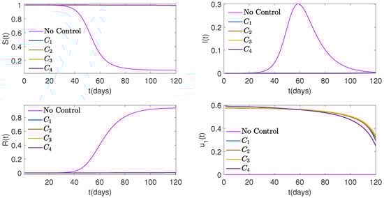
Figure 3. Graphs of Susceptible $S\left(t\right)$ (top on the left), Infected $I\left(t\right)$ (top on the right), and Recovered $R\left(t\right)$ (bottom on the left) people, as well as control $u_1\left(t\right)$ (bottom on the right) over time for four different cost functions $C_1,C_2,C_3,C_4$ versus No Control when weight is ${\lambda }_1=0.001$.

Table 1. Comparison of $\mathcal{I}\left(t\right)$ for cost function $C_1$ in case when only control $u_1$ is applied and ${\lambda }_1$ varies. As ${\lambda }_1$ increases, the number of infected individuals, $\mathcal{I}\left(t\right)$, grows higher on most days.

Day	${\mathit{\lambda }}_1={10}^{-7}$ No 2nd Control	${\mathit{\lambda }}_1=0.001$ No 2nd Control	${\mathit{\lambda }}_1=0.01$ No 2nd Control	${\mathit{\lambda }}_1=0.05$ No 2nd Control	No Control
1	200	200	200	200	200
10	85	253	315	387	1237
20	34	329	527	812	9228
30	15	432	880	1691	67,606
40	7	571	1466	3514	456,639
50	4	761	2447	7267	1,985,292
60	3	1028	4089	14,927	2,987,989
70	2	1416	6873	30,388	2,015,872
80	1	2003	11,678	61,024	1,023,788
90	1	2953	20,264	120,429	474,813
100	1	4643	36,661	233,756	213,085
110	1	8190	72,008	453,110	94,393
120	1	18,714	174,758	922,708	41,578

Table 1. Comparison of $\mathcal{I}\left(t\right)$ for cost function $C_1$ in case when only control $u_1$ is applied and ${\lambda }_1$ varies. As ${\lambda }_1$ increases, the number of infected individuals, $\mathcal{I}\left(t\right)$, grows higher on most days.

Day	${\mathit{\lambda }}_1={10}^{-7}$ No 2nd Control	${\mathit{\lambda }}_1=0.001$ No 2nd Control	${\mathit{\lambda }}_1=0.01$ No 2nd Control	${\mathit{\lambda }}_1=0.05$ No 2nd Control	No Control
1	200	200	200	200	200
10	85	253	315	387	1237
20	34	329	527	812	9228
30	15	432	880	1691	67,606
40	7	571	1466	3514	456,639
50	4	761	2447	7267	1,985,292
60	3	1028	4089	14,927	2,987,989
70	2	1416	6873	30,388	2,015,872
80	1	2003	11,678	61,024	1,023,788
90	1	2953	20,264	120,429	474,813
100	1	4643	36,661	233,756	213,085
110	1	8190	72,008	453,110	94,393
120	1	18,714	174,758	922,708	41,578

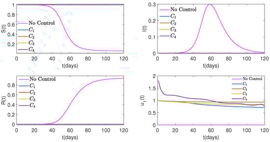
Figure 4. Graphs of Susceptible $S\left(t\right)$ (top on the left), Infected $I\left(t\right)$ (top on the right), and Recovered $R\left(t\right)$ (bottom on the left) people, as well as control $u_1\left(t\right)$ (bottom on the right) over time for four different cost functions $C_1,C_2,C_3,C_4$ versus No Control when weight is ${\lambda }_1={10}^{-7}$. For the cost function $C_4$, $u_1\left(t\right)$ stayed above the ultimate value, $u_1\left(t\right)=1$, for more than half of the study period, which is not practical.

4.2. Scenario 2: Control with Antiviral Medication Only

For the next set of experiments, it was assumed that there was only control $u_2\left(t\right)$ in the system. In Figure 5, Figure 6 and Figure 7, one can see the effect of the weight, ${\lambda }_2$, on different cost functions and, as a result, on state variables $S\left(t\right)$, $I\left(t\right)$, and $R\left(t\right)$ over time. Again, as the weight ${\lambda }_2$ decreases, the control played a more effective role in reducing the number of infected people (See Table 2, Table A16, Table A17 and Table A18 for more details).

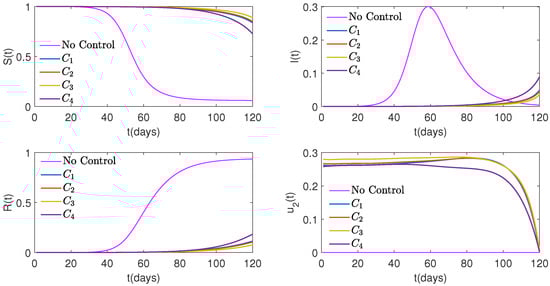
Figure 5. Graphs of Susceptible $S\left(t\right)$ (top on the left), Infected $I\left(t\right)$ (top on the right), and Recovered $R\left(t\right)$ (bottom on the left) people, as well as control $u_2\left(t\right)$ (bottom on the right) over time for four different cost functions $C_1,C_2,C_3,C_4$ versus No Control when weight is $\lambda =0.1$.

Table 2. Comparison of $\mathcal{I}\left(t\right)$ for cost function $C_1$ in case when only control $u_2$ is applied and ${\lambda }_2$ varies. As ${\lambda }_2$ increases, the number of infected individuals, $\mathcal{I}\left(t\right)$, grows higher on most days.

Day	${\mathit{\lambda }}_2={10}^{-7}$ No 1st Control	${\mathit{\lambda }}_2=0.001$ No 1st Control	${\mathit{\lambda }}_2=0.01$ No 1st Control	${\mathit{\lambda }}_2=0.05$ No 1st Control	${\mathit{\lambda }}_2=0.1$ No 1st Control	No Control
1	200	200	200	200	200	200
10	18	181	254	318	377	1237
20	1	168	332	530	756	9228
30	0	164	437	880	1503	67,606
40	0	166	581	1456	2949	456,639
50	0	177	782	2395	5693	1,985,292
60	0	198	1073	3938	10,735	2,987,989
70	0	234	1515	6481	19,547	2,015,872
80	0	299	2226	10,735	34,005	1,023,788
90	0	420	3485	18,210	56,943	474,813
100	0	676	6092	33,048	95,559	213,085
110	0	1391	13,102	70,339	177,085	94,393
120	0	5265	49,724	244,998	499,616	41,578

Table 2. Comparison of $\mathcal{I}\left(t\right)$ for cost function $C_1$ in case when only control $u_2$ is applied and ${\lambda }_2$ varies. As ${\lambda }_2$ increases, the number of infected individuals, $\mathcal{I}\left(t\right)$, grows higher on most days.

Day	${\mathit{\lambda }}_2={10}^{-7}$ No 1st Control	${\mathit{\lambda }}_2=0.001$ No 1st Control	${\mathit{\lambda }}_2=0.01$ No 1st Control	${\mathit{\lambda }}_2=0.05$ No 1st Control	${\mathit{\lambda }}_2=0.1$ No 1st Control	No Control
1	200	200	200	200	200	200
10	18	181	254	318	377	1237
20	1	168	332	530	756	9228
30	0	164	437	880	1503	67,606
40	0	166	581	1456	2949	456,639
50	0	177	782	2395	5693	1,985,292
60	0	198	1073	3938	10,735	2,987,989
70	0	234	1515	6481	19,547	2,015,872
80	0	299	2226	10,735	34,005	1,023,788
90	0	420	3485	18,210	56,943	474,813
100	0	676	6092	33,048	95,559	213,085
110	0	1391	13,102	70,339	177,085	94,393
120	0	5265	49,724	244,998	499,616	41,578

Overall, the effects of controls $u_1\left(t\right)$ and $u_2\left(t\right)$ on the system, when only one control was applied, were similar. However, as one can clearly see from Table 3, for the same cost and over the same time interval, control $u_2\left(t\right)$ suppressed infections more aggressively than $u_1\left(t\right)$. Also, there is a significant difference between the results for cost function $C_4\left(u\right)$ and the rest of the cost functions. While for $C_1\left(u\right)$, $C_2\left(u\right)$, and $C_3\left(u\right)$ the maximum number of infected people on any given day in the case of “first control only” was 923,332, this number was 1,511,537 for $C_4\left(u\right)$. Additionally, in the case of “second control only”, the maximum daily number of infected individuals for $C_4\left(u\right)$ exceeded the maximum daily number for other cost functions by 154,151 cases.

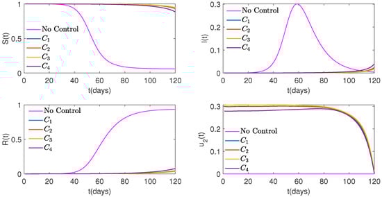
Figure 6. Graphs of Susceptible $S\left(t\right)$ (top on the left), Infected $I\left(t\right)$ (top on the right), and Recovered $R\left(t\right)$ (bottom on the left) people, as well as control $u_2\left(t\right)$ (bottom on the right) over time for four different cost functions $C_1,C_2,C_3,C_4$ versus No Control when weight is ${\lambda }_2=0.05$.

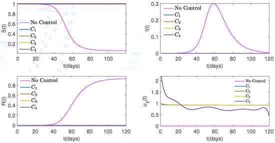
Figure 7. Graphs of Susceptible $S\left(t\right)$ (top on the left), Infected $I\left(t\right)$ (top on the right), and Recovered $R\left(t\right)$ (bottom on the left) people, as well as control $u_2\left(t\right)$ (bottom on the right) over time for four different cost functions $C_1,C_2,C_3,C_4$ versus No Control when weight is ${\lambda }_2={10}^{-7}$.

The best performance among all cost functions can be attributed to $C_3\left(u\right)$ in both cases where only control $u_1\left(t\right)$ or only control $u_2\left(t\right)$ was applied. For details, one can see Table 3 and Figure 8.

Table 3. Comparison of $\mathcal{I}\left(t\right)$ for all cost functions in the case when only control $u_1$ is applied (${\lambda }_1=0.05$) or only control $u_2$ is applied (${\lambda }_2=0.05$) over time.

Day	${\mathit{\lambda }}_1=0.05$ No 2nd Control	No 1st Control ${\mathit{\lambda }}_2=0.05$	${\mathit{\lambda }}_1=0.05$ No 2nd Control	No 1st Control ${\mathit{\lambda }}_2=0.05$	${\mathit{\lambda }}_1=0.05$ No 2nd Control	No 1st Control ${\mathit{\lambda }}_2=0.05$	${\mathit{\lambda }}_1=0.05$ No 2nd Control	No 1st Control ${\mathit{\lambda }}_2=0.05$
	${\mathit{C}}_{\mathbf{1}}$		${\mathit{C}}_{\mathbf{2}}$		${\mathit{C}}_{\mathbf{3}}$		${\mathit{C}}_{\mathbf{4}}$
1	200	200	200	200	200	200	200	200
10	387	318	388	317	377	308	401	349
20	812	530	816	527	766	495	918	644
30	1691	880	1706	872	1552	795	2133	1178
40	3514	1456	3557	1439	3134	1273	4939	2133
50	7267	2395	7379	2362	6302	2034	11,366	3816
60	14,927	3938	15,209	3879	12,618	3258	25,851	6733
70	30,388	6481	31,076	6381	25,120	5256	57,953	11,672
80	61,024	10,735	6,2623	10,561	49,586	8558	127,302	19,877
90	120,429	18,210	123,913	17,880	96,926	14,338	266,304	33,825
100	233,756	33,048	240,619	32,336	188,180	25,768	509,874	60,100
110	453,110	70,339	463,527	67,697	367,745	53,756	899,275	123,379
120	922,708	244,998	923,332	229,683	760,101	183,048	1,511,537	399,149

Table 3. Comparison of $\mathcal{I}\left(t\right)$ for all cost functions in the case when only control $u_1$ is applied (${\lambda }_1=0.05$) or only control $u_2$ is applied (${\lambda }_2=0.05$) over time.

Day	${\mathit{\lambda }}_1=0.05$ No 2nd Control	No 1st Control ${\mathit{\lambda }}_2=0.05$	${\mathit{\lambda }}_1=0.05$ No 2nd Control	No 1st Control ${\mathit{\lambda }}_2=0.05$	${\mathit{\lambda }}_1=0.05$ No 2nd Control	No 1st Control ${\mathit{\lambda }}_2=0.05$	${\mathit{\lambda }}_1=0.05$ No 2nd Control	No 1st Control ${\mathit{\lambda }}_2=0.05$
	${\mathit{C}}_{\mathbf{1}}$		${\mathit{C}}_{\mathbf{2}}$		${\mathit{C}}_{\mathbf{3}}$		${\mathit{C}}_{\mathbf{4}}$
1	200	200	200	200	200	200	200	200
10	387	318	388	317	377	308	401	349
20	812	530	816	527	766	495	918	644
30	1691	880	1706	872	1552	795	2133	1178
40	3514	1456	3557	1439	3134	1273	4939	2133
50	7267	2395	7379	2362	6302	2034	11,366	3816
60	14,927	3938	15,209	3879	12,618	3258	25,851	6733
70	30,388	6481	31,076	6381	25,120	5256	57,953	11,672
80	61,024	10,735	6,2623	10,561	49,586	8558	127,302	19,877
90	120,429	18,210	123,913	17,880	96,926	14,338	266,304	33,825
100	233,756	33,048	240,619	32,336	188,180	25,768	509,874	60,100
110	453,110	70,339	463,527	67,697	367,745	53,756	899,275	123,379
120	922,708	244,998	923,332	229,683	760,101	183,048	1,511,537	399,149

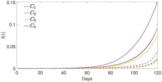
Figure 8. Graphs of $I\left(t\right)$ for different cost functions $C_1,C_2,C_3,C_4$ when only $u_1\left(t\right)$ is applied and ${\lambda }_1=0.05$ (shown with solid lines), as well as when only $u_2\left(t\right)$ is applied and ${\lambda }_2=0.05$ (shown with dashed line).

4.3. Scenario 3: Non-Medical and Medical Controls in Combination

For the next step, we applied two controls to the $SIR$ system, $u_1\left(t\right)$ and $u_2\left(t\right)$, together with the same weights, ${\lambda }_1={\lambda }_2=\lambda$, in order to evaluate their effect on the outbreak (See Figure 9, Figure 10, Figure 11 and Figure 12). As expected, in terms of its dependence on $\lambda$, the combination of two controls, $u_1\left(t\right)$ and $u_2\left(t\right)$, behaved pretty similar to the case of one control in a sense that when the weight $\lambda$ decreased, the controls became more effective, and the daily number of infected humans went down.

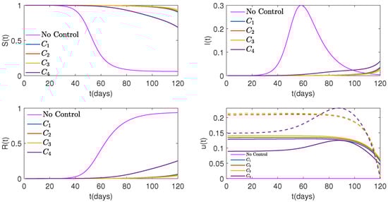
Figure 9. Graphs of Susceptible $S\left(t\right)$ (top on the left), Infected $I\left(t\right)$ (top on the right), Recovered $R\left(t\right)$ (bottom on the left) people, controls $u_1\left(t\right)$ shown with solid lines, and $u_2\left(t\right)$ with dashed lines (bottom on the right) over time for four different cost functions $C_1,C_2,C_3,C_4$ versus No Control when weights, ${\lambda }_1$, and ${\lambda }_2$, for both controls are $0.1$.

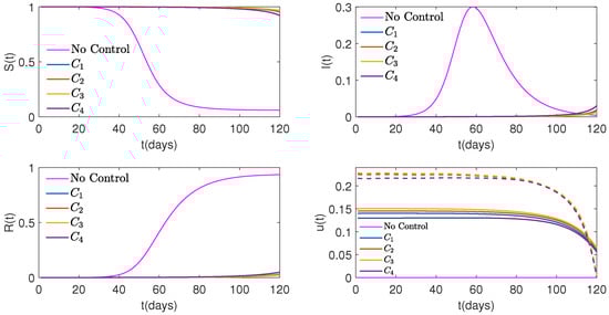
Figure 10. Graphs of Susceptible $S\left(t\right)$ (top on the left), Infected $I\left(t\right)$ (top on the right), Recovered $R\left(t\right)$ (bottom on the left) people, control $u_1$ shown with solid lines, and $u_2$ with dashed lines (bottom on the right) over time for four different cost functions $C_1,C_2,C_3,C_4$ versus No Control when weight, $\lambda$, for both controls is ${\lambda }_1={\lambda }_2=\lambda =0.05$.

Table 4 and Table 5 show the daily number of infected individuals, $\mathcal{I}\left(t\right)$, and the cumulative number of infected individuals up to day t, $N-\mathcal{S}\left(t\right)$, for different control scenarios. This gives an insight into how the two controls, $u_1\left(t\right)$ and $u_2\left(t\right)$, compare individually and in combination when subject to the same cost, $C_1\left(u\right)$, and the same weight, ${\lambda }_1={\lambda }_2=\lambda =0.05$. Table 5 illustrates that the cumulative number of infections after applying both controls for 120 days was 454,205, while the “no control” counterpart was 9,397,865. And in the case of the control with antiviral medication, $u_2\left(t\right)$, after 120 days, there were more than the times fewer cases compared to the case of social distancing control, $u_1\left(t\right)$ (692,160 vs. 2,256,854). Similar tables related to the cost functions $C_2\left(u\right)$, $C_3\left(u\right)$, and $C_4\left(u\right)$ can be found in Appendix A (Table A1, Table A2, Table A3, Table A4, Table A5 and Table A6).

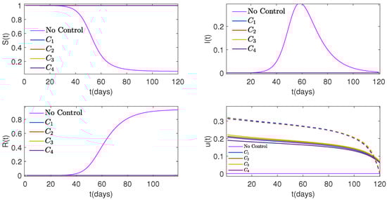
Figure 11. Graphs of Susceptible $S\left(t\right)$ (top on the left), Infected $I\left(t\right)$ (top on the right), Recovered $R\left(t\right)$ (bottom on the left) people, controls $u_1\left(t\right)$ shown with solid lines, and $u_2\left(t\right)$ with dashed lines (bottom on the right) over time for four different cost functions $C_1,C_2,C_3,C_4$ versus No Control when weight, $\lambda$, for both controls is ${\lambda }_1={\lambda }_2=\lambda =0.001$.

Table 4. Comparison of $\mathcal{I}\left(t\right)$ for cost function $C_1$ when there is only $u_1$, only $u_2$, and both $u_1,u_2$ applied versus No Control case over time when $\lambda =0.05$.

Day	No Control	${\mathit{\lambda }}_1=0.05$ No 2nd Control	No 1st Control ${\mathit{\lambda }}_2=0.05$	${\mathit{\lambda }}_1=0.05$ ${\mathit{\lambda }}_2=0.05$
1	200	200	200	200
10	1237	387	318	300
20	9228	812	530	472
30	67,606	1691	880	743
40	456,639	3514	1456	1167
50	1,985,292	7267	2395	1834
60	2,987,989	14,927	3938	2897
70	2,015,872	30,388	6481	4625
80	1,023,788	61,024	10,735	7522
90	474,813	120,429	18,210	12,727
100	213,085	233,756	33,048	23,355
110	94,393	453,110	70,339	50,792
120	41,578	922,708	244,998	173,543

Table 4. Comparison of $\mathcal{I}\left(t\right)$ for cost function $C_1$ when there is only $u_1$, only $u_2$, and both $u_1,u_2$ applied versus No Control case over time when $\lambda =0.05$.

Day	No Control	${\mathit{\lambda }}_1=0.05$ No 2nd Control	No 1st Control ${\mathit{\lambda }}_2=0.05$	${\mathit{\lambda }}_1=0.05$ ${\mathit{\lambda }}_2=0.05$
1	200	200	200	200
10	1237	387	318	300
20	9228	812	530	472
30	67,606	1691	880	743
40	456,639	3514	1456	1167
50	1,985,292	7267	2395	1834
60	2,987,989	14,927	3938	2897
70	2,015,872	30,388	6481	4625
80	1,023,788	61,024	10,735	7522
90	474,813	120,429	18,210	12,727
100	213,085	233,756	33,048	23,355
110	94,393	453,110	70,339	50,792
120	41,578	922,708	244,998	173,543

In the next series of experiments, controls $u_1\left(t\right)$ and $u_2\left(t\right)$ had different weights, ${\lambda }_1$ and ${\lambda }_2$, applied to their respective cost functions. We considered two cases. First, for the cost function $C_1\left(u\right)$, the weight of control $u_1\left(t\right)$ was less than the weight of control $u_2\left(t\right)$ (${\lambda }_1<{\lambda }_2$). Table 6 shows the changes in the daily numbers of infected people, $\mathcal{I}\left(t\right)$, for the cost function $C_1\left(u\right)$, in the case of fixed weight (${\lambda }_1=0.05$) for control $u_1\left(t\right)$ and different weights for control $u_2\left(t\right)$ (Table A7, Table A8 and Table A9 for cost functions $C_2\left(u\right),C_3\left(u\right)$, and $C_4\left(u\right)$ can be found in Appendix A). As it follows from Table 6, adding the second control, $u_2\left(t\right)$, with any weight, ${\lambda }_2$, helped to better contain the outbreak and to decrease the daily number of infected people, as well as the cumulative number of cases. Even for a high effort case of ${\lambda }_2=0.1$, the number of daily infections was $\mathrm{624,040}$ cases less than the daily number of infected individuals in the case when there was no control: $u_2\left(t\right)$. However, when the weight of the second control ${\lambda }_2$ increased, the effort required to implement that measure also rose, making it increasingly challenging to execute. When the roles were reversed, that is, for the cost function $C_1\left(u\right)$, the weight, ${\lambda }_2=0.05$, of the second control $u_2\left(t\right)$ was fixed, and the sensitivity of the system to the first control $u_1\left(t\right)$ was observed, the pattern ended up being similar. Namely, adding a non-medical control, $u_1\left(t\right)$, reduced the daily number of infected people. Even though it was not as consequential as in the case when control $u_2\left(t\right)$ was added, there were still fewer infected people in all cases with two controls as opposed to the case of $u_2\left(t\right)$ only. At the same time, it is evident that the second control, $u_2\left(t\right)$, is more efficient. Indeed, for the high effort case of ${\lambda }_1=0.1$, the number of daily infections was only $\mathrm{44,983}$ cases less than the daily number of infected individuals in the case when there was no control $u_1\left(t\right)$ (as opposed to a $\mathrm{624,040}$ reduction when $u_2\left(t\right)$ was added with the same effort of $0.1$). The difference in the daily number of infected individuals between the case of no $u_1\left(t\right)$ (i.e., $u_2\left(t\right)$ only with weight ${\lambda }_1=0.05$) and the case of $u_2\left(t\right)$ with ${\lambda }_1=0.05$ and $u_1\left(t\right)$ with varying weights ranged from $\mathrm{244,998}$ to $\mathrm{16,608}$. See Table 7, Table A10, Table A11 and Table A12 for more details.

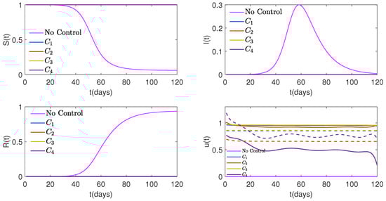
Figure 12. Graphs of Susceptible $S\left(t\right)$ (top on the left), Infected $I\left(t\right)$ (top on the right), Recovered $R\left(t\right)$ (bottom on the left) people, controls $u_1\left(t\right)$ shown with solid lines, and $u_2\left(t\right)$ with dashed lines (bottom on the right) for four different cost functions $C_1,C_2,C_3,C_4$ versus No Control when weight, $\lambda$, for both controls is ${\lambda }_1={\lambda }_2=\lambda ={10}^{-8}$. Control $u_2$ for cost function $C_4$ takes unrealistic values above 1 at the early period of the study.

Figure 13 and Figure 14 show the behaviors of the controls and their effects on the graphs of $I\left(t\right)$ for different cost functions and different weights. As is evident from the graphs, when ${\lambda }_1=0.05$ and ${\lambda }_2=0.01$, the second control, $u_2\left(t\right)$, was dominant and very efficient. At the same time, when ${\lambda }_1=0.05$ and ${\lambda }_2=0.1$, the two controls, $u_1\left(t\right)$ and $u_2\left(t\right)$, were about the same, and there were more infected people toward the end of the study period, that is, the control strategy in Figure 14 is less efficient compared to the case of Figure 13. The two figures, once again, underline the significance of the second control $u_2\left(t\right)$.

Table 5. Cumulative number of infections up to day t, $N-\mathcal{S}\left(t\right)$ for cost function $C_1$ when there is only $u_1$, only $u_2$, and both $u_1,u_2$ versus No Control case over time when weight ${\lambda }_1={\lambda }_2=\lambda =0.05$.

Day	No Control	${\mathit{\lambda }}_1=0.05$ No 2nd Control	No 1st Control ${\mathit{\lambda }}_2=0.05$	${\mathit{\lambda }}_1=0.05$ ${\mathit{\lambda }}_2=0.05$
1	200	200	200	200
10	1756	643	898	772
20	13,747	1649	2156	1761
30	101,568	3735	4239	3312
40	697,572	8067	7686	5748
50	3,338,392	17,006	13,356	9562
60	7,032,920	35,334	22,686	15,568
70	8,627,485	72,609	37,993	25,108
80	9,121,747	147,335	63,222	40,496
90	9,292,217	294,458	105,246	66,067
100	9,358,556	579,209	178,417	111,270
110	9,386,082	1,130,270	320,258	202,389
120	9,397,865	2,256,854	692,160	454,205

Table 5. Cumulative number of infections up to day t, $N-\mathcal{S}\left(t\right)$ for cost function $C_1$ when there is only $u_1$, only $u_2$, and both $u_1,u_2$ versus No Control case over time when weight ${\lambda }_1={\lambda }_2=\lambda =0.05$.

Day	No Control	${\mathit{\lambda }}_1=0.05$ No 2nd Control	No 1st Control ${\mathit{\lambda }}_2=0.05$	${\mathit{\lambda }}_1=0.05$ ${\mathit{\lambda }}_2=0.05$
1	200	200	200	200
10	1756	643	898	772
20	13,747	1649	2156	1761
30	101,568	3735	4239	3312
40	697,572	8067	7686	5748
50	3,338,392	17,006	13,356	9562
60	7,032,920	35,334	22,686	15,568
70	8,627,485	72,609	37,993	25,108
80	9,121,747	147,335	63,222	40,496
90	9,292,217	294,458	105,246	66,067
100	9,358,556	579,209	178,417	111,270
110	9,386,082	1,130,270	320,258	202,389
120	9,397,865	2,256,854	692,160	454,205

Table 6. Comparison of the daily number of infected people, $\mathcal{I}\left(t\right)$, for the cost function $C_1$ with the weight ${\lambda }_1=0.05$ for $u_1\left(t\right)$. The weights for the control $u_2\left(t\right)$ are ${\lambda }_2=0.001$, $0.01$, $0.05$, and $0.1$ for the second, third, and fourth columns, respectively, and the fifth column shows the case of No Control $u_2\left(t\right)$ over time.

Day	${\mathit{\lambda }}_1=0.05$ ${\mathit{\lambda }}_2=0.001$	${\mathit{\lambda }}_1=0.05$ ${\mathit{\lambda }}_2=0.01$	${\mathit{\lambda }}_1=0.05$ ${\mathit{\lambda }}_2=0.05$	${\mathit{\lambda }}_1=0.05$ ${\mathit{\lambda }}_2=0.1$	${\mathit{\lambda }}_1=0.05$ No 2nd Control
1	200	200	200	200	200
10	180	251	300	321	387
20	167	323	472	545	812
30	163	421	743	925	1691
40	165	554	1167	1561	3514
50	175	737	1834	2629	7267
60	195	1002	2897	4428	14,927
70	231	1404	4625	7481	30,388
80	291	2049	7522	12,748	61,024
90	403	3188	12,727	22,274	120,429
100	646	5554	23,355	41,465	233,756
110	1306	11,909	50,792	89,010	453,110
120	4879	44,363	173,543	280,668	922,708

Table 6. Comparison of the daily number of infected people, $\mathcal{I}\left(t\right)$, for the cost function $C_1$ with the weight ${\lambda }_1=0.05$ for $u_1\left(t\right)$. The weights for the control $u_2\left(t\right)$ are ${\lambda }_2=0.001$, $0.01$, $0.05$, and $0.1$ for the second, third, and fourth columns, respectively, and the fifth column shows the case of No Control $u_2\left(t\right)$ over time.

Day	${\mathit{\lambda }}_1=0.05$ ${\mathit{\lambda }}_2=0.001$	${\mathit{\lambda }}_1=0.05$ ${\mathit{\lambda }}_2=0.01$	${\mathit{\lambda }}_1=0.05$ ${\mathit{\lambda }}_2=0.05$	${\mathit{\lambda }}_1=0.05$ ${\mathit{\lambda }}_2=0.1$	${\mathit{\lambda }}_1=0.05$ No 2nd Control
1	200	200	200	200	200
10	180	251	300	321	387
20	167	323	472	545	812
30	163	421	743	925	1691
40	165	554	1167	1561	3514
50	175	737	1834	2629	7267
60	195	1002	2897	4428	14,927
70	231	1404	4625	7481	30,388
80	291	2049	7522	12,748	61,024
90	403	3188	12,727	22,274	120,429
100	646	5554	23,355	41,465	233,756
110	1306	11,909	50,792	89,010	453,110
120	4879	44,363	173,543	280,668	922,708

Table 7. Comparison of the daily number of infected people, $\mathcal{I}\left(t\right)$, for the cost function $C_1$ with the weight ${\lambda }_2=0.05$ for $u_2\left(t\right)$. The weights for the control $u_1\left(t\right)$ are ${\lambda }_1=0.001$, $0.01$, $0.05$, and $0.1$ for the second, third, and fourth columns, respectively, and the fifth column shows the case of No Control $u_1\left(t\right)$ over time.

Day	${\mathit{\lambda }}_1=0.001$ ${\mathit{\lambda }}_2=0.05$	${\mathit{\lambda }}_1=0.01$ ${\mathit{\lambda }}_2=0.05$	${\mathit{\lambda }}_1=0.05$ ${\mathit{\lambda }}_2=0.05$	${\mathit{\lambda }}_1=0.1$ ${\mathit{\lambda }}_2=0.05$	No 1st Control ${\mathit{\lambda }}_2=0.05$
1	200	200	200	200	200
10	245	281	300	306	318
20	308	411	472	492	530
30	390	604	743	791	880
40	500	890	1167	1268	1456
50	649	1318	1834	2028	2395
60	857	1976	2897	3253	3938
70	1159	3016	4625	5258	6481
80	1621	4732	7522	8613	10,735
90	2383	7788	12,727	14,602	18,210
100	3777	13,962	23,355	26,759	33,048
110	6844	29,381	50,792	57,816	70,339
120	16,608	90,271	173,543	200,015	244,998

Table 7. Comparison of the daily number of infected people, $\mathcal{I}\left(t\right)$, for the cost function $C_1$ with the weight ${\lambda }_2=0.05$ for $u_2\left(t\right)$. The weights for the control $u_1\left(t\right)$ are ${\lambda }_1=0.001$, $0.01$, $0.05$, and $0.1$ for the second, third, and fourth columns, respectively, and the fifth column shows the case of No Control $u_1\left(t\right)$ over time.

Day	${\mathit{\lambda }}_1=0.001$ ${\mathit{\lambda }}_2=0.05$	${\mathit{\lambda }}_1=0.01$ ${\mathit{\lambda }}_2=0.05$	${\mathit{\lambda }}_1=0.05$ ${\mathit{\lambda }}_2=0.05$	${\mathit{\lambda }}_1=0.1$ ${\mathit{\lambda }}_2=0.05$	No 1st Control ${\mathit{\lambda }}_2=0.05$
1	200	200	200	200	200
10	245	281	300	306	318
20	308	411	472	492	530
30	390	604	743	791	880
40	500	890	1167	1268	1456
50	649	1318	1834	2028	2395
60	857	1976	2897	3253	3938
70	1159	3016	4625	5258	6481
80	1621	4732	7522	8613	10,735
90	2383	7788	12,727	14,602	18,210
100	3777	13,962	23,355	26,759	33,048
110	6844	29,381	50,792	57,816	70,339
120	16,608	90,271	173,543	200,015	244,998

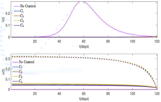
Figure 13. The proportion of infected people, $I\left(t\right)$, for different cost functions and No Control case when ${\lambda }_1=0.05,{\lambda }_2=0.01$ (on the top) and controls $u_1\left(t\right)$ shown with solid lines, with $u_2\left(t\right)$ shown with dashed lines (on the bottom).

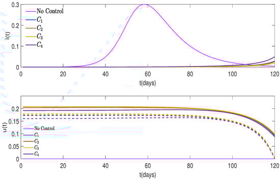
Figure 14. The proportion of infected people, $I\left(t\right)$, for different cost functions and No Control case when ${\lambda }_1=0.05,{\lambda }_2=0.1$ (on the top) and controls $u_1\left(t\right)$ shown with solid lines, with $u_2\left(t\right)$ shown with dashed lines (on the bottom).

5. Conclusions

To summarize, in this study, we investigated different control scenarios through theoretical analysis and numerical simulations. To account for two important types of control, social distancing and treatment with antiviral medications, the $SIR$ (Susceptible-Infectious-Removed) model [19] for an early ascending stage of an outbreak has been considered with the first control $u_1\left(t\right)$—aimed at lowering the disease transmission rate—and the second control $u_2\left(t\right)$—aimed at lowering the period of infectiousness. In all experiments, the implementation of control strategies reduced the daily cumulative number of cases, $N-\mathcal{S}\left(t\right)$, and successfully “flattened the curve”, $\mathcal{I}\left(t\right)$. The reduction in the cumulative cases was achieved by eliminating or delaying new cases. This delay is incredibly valuable, as it provides public health organizations with more time to advance antiviral treatments and devise alternative preventive measures.

The main theoretical result of this paper, Theorem 1, concludes that the optimal control functions, $u_i\left(t\right)$ and $i=1,2,$ may be increasing until some moment $\tau \in [0,T)$. However, for all $t\in [\tau ,T]$, the derivatives, ${\displaystyle \frac{d{u}_i}{dt}}$, become negative, and both controls, $u_i\left(t\right)$, decline as t approaches T (possibly causing the number of newly infected people to grow). The numerical simulations presented in Section 4 confirm our theoretical findings. So ideally around the time $t=\tau$, preventive measures have to be upgraded, and vaccination campaigns need to start to ensure that the epidemic wave does not rebound. The period from 0 to $\tau$ must be used by scientists and public health professionals to effectively implement early control strategies but also to develop new and improved tools, such as vaccines, therapeutics, testing, air ventilation, and others, to successfully battle the virus beyond the point $t=\tau$.

Appendix A.1. Properties of SIR Model with Time-Dependent Coefficients

In Section 3, it has been pointed out that even though for system (2), the effective reproduction number, $r\left(t\right)=\beta (1-u_1\left(t\right))/(\gamma +\epsilon u_2\left(t\right))$, reduces with more control, it does not guarantee that $r\left(t\right)\ge \overline{r}\left(t\right)$ yields $S\left(t\right)\le \overline{S}\left(t\right)$ for every value of t. One can, however, show that if $r\left(t\right)\ge \overline{r}\left(t\right)$ and $r\left(t\right)$ are non-increasing, then $S\left(t\right)\le \overline{S}\left(t\right)$. The proof of this result is given below.

Theorem A1.

Assume that ${\displaystyle \frac{d\mathbf{x}}{dt}}=f(\mathbf{x},\beta ,\gamma )$, $\mathbf{x}\left(0\right)={\mathbf{x}}_0$, where $\mathbf{x}\left(t\right)={[S\left(t\right),I\left(t\right),R\left(t\right)]}^{\top }$,

$$\begin{array}{ll}{f}_1(\mathbf{x},\beta ,\gamma )& :=-\beta \left(t\right)S\left(t\right)I\left(t\right)\\ f_2(\mathbf{x},\beta ,\gamma )& :=\beta \left(t\right)S\left(t\right)I\left(t\right)-\gamma \left(t\right)I\left(t\right)\\ f_3(\mathbf{x},\beta ,\gamma )& :=\gamma \left(t\right)I\left(t\right),\end{array}$$

(A1)

$$and{\mathbf{x}}_0\in {\Delta }^2:=\{(z_1,z_2,z_3)\in {\mathbb{R}}^3:z_1+z_2+z_3=1,z_1,z_2,z_3\ge 0\}.$$

(A2)

Let $\mathbf{x}\left(t\right)$ and $\widehat{\mathbf{x}}\left(t\right)$ satisfy ${\displaystyle \frac{d\mathbf{x}}{dt}}=f(\mathbf{x},\beta ,\gamma )$ and ${\displaystyle \frac{d\widehat{\mathbf{x}}}{dt}}=f(\widehat{\mathbf{x}},\widehat{\beta },\widehat{\gamma })$, respectively, with the same initial condition ${\mathbf{x}}_0={\widehat{\mathbf{x}}}_0={[S_0,I_0,R_0]}^{\top }$, $R_0\ge 0$, $S_0,I_0>0$, $\beta \left(t\right),\gamma \left(t\right),\widehat{\beta }\left(t\right),\widehat{\gamma }\left(t\right)>0$ for any $t\in [0,T]$, and $\beta \left(0\right)>\widehat{\beta }\left(0\right)>0$. Suppose that $r\left(t\right):=\beta \left(t\right)/\gamma \left(t\right)$, $\widehat{r}\left(t\right):=\widehat{\beta }\left(t\right)/\widehat{\gamma }\left(t\right)$, and $r\left(t\right)\ge \widehat{r}\left(t\right)$ for all $t\in [0,T]$. If $r\left(t\right)\in {\mathcal{L}}^1[0,T]$ and $r\left(t\right)$ are non-increasing, then $S\left(t\right)\le \widehat{S}\left(t\right)$ for any $t\in [0,T]$.

Proof. 

Since ${\mathbf{x}}_0={\widehat{\mathbf{x}}}_0$, $S_0,I_0>0$ and $\beta \left(0\right)>\widehat{\beta }\left(0\right)$, so one concludes that $S_0={\widehat{S}}_0>0$, $I_0={\widehat{I}}_0>0$, and $\beta \left(0\right)S_0{I}_0>\widehat{\beta }\left(0\right){\widehat{S}}_0{\widehat{I}}_0$. Therefore, according to (A1), $S^{\prime }\left(0\right)<{\widehat{S}}^{\prime }\left(0\right)$, and there exists $ϵ>0$ such that $S\left(t\right)<\widehat{S}\left(t\right)$ for any $t\in (0,ϵ]$. If the claim does not hold, then there is $\mu >ϵ$ such that $S\left(\mu \right)>\widehat{S}\left(\mu \right)$. According to the intermediate value theorem, there exists $\tau \in (ϵ,\mu )$ such that

$$\begin{array}{cc}S\left(t\right)<\widehat{S}\left(t\right)& \mathrm{for} \mathrm{any}t\in (0,\tau )\\ S\left(\tau \right)=\widehat{S}\left(\tau \right)& \mathrm{and}{S}^{\prime }\left(\tau \right)\ge {\widehat{S}}^{\prime }\left(\tau \right).\end{array}$$

(A3)

From (A3), one obtains

$$S^{\prime }\left(\tau \right)=-\beta \left(\tau \right)S\left(\tau \right)I\left(\tau \right)>-\widehat{\beta }\left(\tau \right)\widehat{S}\left(\tau \right)\widehat{I}\left(\tau \right)=S^{\prime }\left(\tau \right),$$

(A4)

that is,

$$I\left(\tau \right)\le \widehat{I}\left(\tau \right).$$

(A5)

On the other hand, according to (A2),

$$I\left(\tau \right)-\widehat{I}\left(\tau \right)=1-S\left(\tau \right)-R\left(\tau \right)-(1-\widehat{S}\left(\tau \right)-\widehat{R}\left(\tau \right))=\widehat{R}\left(\tau \right)-R\left(\tau \right).$$

(A6)

As it follows from (A1),

$${(lnS\left(t\right))}^{\prime }=-\beta \left(t\right)I\left(t\right)=-{\displaystyle \frac{\beta \left(t\right)}{\gamma \left(t\right)}}{R}^{\prime }\left(t\right)=-r\left(t\right)R^{\prime }\left(t\right).$$

(A7)

This yields

$$R\left(\tau \right)=R_0+{\int }_0^{\tau }{R}^{\prime }\left(t\right)dt=R_0-{\int }_0^{\tau }{\displaystyle \frac{{(lnS\left(t\right))}^{\prime }}{r\left(t\right)}}dt.$$

(A8)

Identities (A7) and (A8) imply that

$$\begin{array}{ll}I\left(\tau \right)-\widehat{I}\left(\tau \right)& ={\int }_0^{\tau }\left\{{\displaystyle \frac{{(lnS\left(t\right))}^{\prime }}{r\left(t\right)}}-{\displaystyle \frac{{(ln\widehat{S}\left(t\right))}^{\prime }}{\widehat{r}\left(t\right)}}\right\}dt={\int }_0^{\tau }{\displaystyle \frac{{(lnS\left(t\right))}^{\prime }-{(ln\widehat{S}\left(t\right))}^{\prime }}{r\left(t\right)}}dt\\ & ={\int }_0^{\tau }\left\{{\displaystyle \frac{1}{r\left(t\right)}}-{\displaystyle \frac{1}{\widehat{r}\left(t\right)}}\right\}{(ln\widehat{S}\left(t\right))}^{\prime }dt:={\mathcal{T}}_1+{\mathcal{T}}_2.\end{array}$$

(A9)

Since $r\left(t\right)\in {\mathcal{L}}^1[0,T]$ is non-increasing, $S\left(t\right)<\widehat{S}\left(t\right)$ for any $t\in (0,\tau )$, $S\left(0\right)=\widehat{S}\left(0\right)$, and $S\left(\tau \right)=\widehat{S}\left(\tau \right)$; according to the intermediate value theorem for the first term in (A9), one has

$$\begin{array}{ll}{\mathcal{T}}_1& ={\int }_0^{\tau }{\displaystyle \frac{{(lnS\left(t\right))}^{\prime }-{(ln\widehat{S}\left(t\right))}^{\prime }}{r\left(t\right)}}dt={\left.{\displaystyle \frac{lnS\left(t\right)-ln\widehat{S}\left(t\right)}{r\left(t\right)}}\right|}_0^{\tau }+{\int }_0^{\tau }\left\{lnS\left(t\right)-ln\widehat{S}\left(t\right)\right\}{\displaystyle \frac{r^{\prime }\left(t\right)}{r^2\left(t\right)}}dt\\ & =-{\displaystyle \frac{r^{\prime }\left(\nu \right)}{r^2\left(\nu \right)}}{\int }_0^{\tau }\left\{ln\widehat{S}\left(t\right)-lnS\left(t\right)\right\}dt\ge 0,\end{array}$$

(A10)

where $\nu \in [0,\tau ]$. Furthermore, according to Lemma 1, $S\left(t\right),I\left(t\right)>0$ and ${(lnS\left(t\right))}^{\prime }<0$ for any $t\in [0,T]$. Hence, from $r\left(t\right)\ge \widehat{r}\left(t\right)$, it follows that

$$\begin{array}{ll}{\mathcal{T}}_2& ={\int }_0^{\tau }\left\{{\displaystyle \frac{1}{r\left(t\right)}}-{\displaystyle \frac{1}{\widehat{r}\left(t\right)}}\right\}{(ln\widehat{S}\left(t\right))}^{\prime }dt=\left\{{\displaystyle \frac{1}{r\left(\sigma \right)}}-{\displaystyle \frac{1}{\widehat{r}\left(\sigma \right)}}\right\}{\int }_0^{\tau }{(ln\widehat{S}\left(t\right))}^{\prime }dt\\ & =\left\{{\displaystyle \frac{1}{\widehat{r}\left(\sigma \right)}}-{\displaystyle \frac{1}{r\left(\sigma \right)}}\right\}{\displaystyle \frac{\widehat{S}\left(0\right)}{\widehat{S}\left(\tau \right)}}>0.\end{array}$$

(A11)

Combining (A10) and (A11), one concludes that $I\left(\tau \right)>\widehat{I}\left(\tau \right)$, which contradicts (A5). This completes the proof. □

Appendix A.2. Additional Tables

Table A1. Comparison of $\mathcal{I}\left(t\right)$ for cost function $C_2$ when there is only $u_1$, only $u_2$, and both $u_1,u_2$ applied versus No Control case over time when $\lambda =0.05$.

Day	No Control	${\mathit{\lambda }}_1=0.05$ No 2nd Control	No 1st Control ${\mathit{\lambda }}_2=0.05$	${\mathit{\lambda }}_1=0.05$ ${\mathit{\lambda }}_2=0.05$
1	200	200	200	200
10	1237	388	317	298
20	9228	816	527	464
30	67,606	1706	872	725
40	456,639	3557	1439	1132
50	1,985,292	7379	2362	1765
60	2,987,989	15,209	3879	2772
70	2,015,872	31,076	6381	4403
80	1,023,788	62,623	10,561	7122
90	474,813	123,913	17,880	11,975
100	213,085	240,619	32,336	21,814
110	94,393	463,527	67,697	46,675
120	41,578	923,332	229,683	156,190

Table A1. Comparison of $\mathcal{I}\left(t\right)$ for cost function $C_2$ when there is only $u_1$, only $u_2$, and both $u_1,u_2$ applied versus No Control case over time when $\lambda =0.05$.

Day	No Control	${\mathit{\lambda }}_1=0.05$ No 2nd Control	No 1st Control ${\mathit{\lambda }}_2=0.05$	${\mathit{\lambda }}_1=0.05$ ${\mathit{\lambda }}_2=0.05$
1	200	200	200	200
10	1237	388	317	298
20	9228	816	527	464
30	67,606	1706	872	725
40	456,639	3557	1439	1132
50	1,985,292	7379	2362	1765
60	2,987,989	15,209	3879	2772
70	2,015,872	31,076	6381	4403
80	1,023,788	62,623	10,561	7122
90	474,813	123,913	17,880	11,975
100	213,085	240,619	32,336	21,814
110	94,393	463,527	67,697	46,675
120	41,578	923,332	229,683	156,190

Table A2. Comparison of $\mathcal{I}\left(t\right)$ for cost function $C_3$ when there is only $u_1$, only $u_2$, and both $u_1,u_2$ applied versus No Control case over time when $\lambda =0.05$.

Day	No Control	${\mathit{\lambda }}_1=0.05$ No 2nd Control	No 1st Control ${\mathit{\lambda }}_2=0.05$	${\mathit{\lambda }}_1=0.05$ ${\mathit{\lambda }}_2=0.05$
1	200	200	200	200
10	1237	377	308	289
20	9228	766	495	437
30	67,606	1552	795	662
40	456,639	3134	1273	1003
50	1,985,292	6302	2034	1524
60	2,987,989	12,618	3258	2333
70	2,015,872	25,120	5256	3624
80	1,023,788	49,586	8558	5751
90	474,813	96,926	14,338	9523
100	213,085	188,180	25,768	17,140
110	94,393	367,745	53,756	36,352
120	41,578	760,101	183,048	121,390

Table A2. Comparison of $\mathcal{I}\left(t\right)$ for cost function $C_3$ when there is only $u_1$, only $u_2$, and both $u_1,u_2$ applied versus No Control case over time when $\lambda =0.05$.

Day	No Control	${\mathit{\lambda }}_1=0.05$ No 2nd Control	No 1st Control ${\mathit{\lambda }}_2=0.05$	${\mathit{\lambda }}_1=0.05$ ${\mathit{\lambda }}_2=0.05$
1	200	200	200	200
10	1237	377	308	289
20	9228	766	495	437
30	67,606	1552	795	662
40	456,639	3134	1273	1003
50	1,985,292	6302	2034	1524
60	2,987,989	12,618	3258	2333
70	2,015,872	25,120	5256	3624
80	1,023,788	49,586	8558	5751
90	474,813	96,926	14,338	9523
100	213,085	188,180	25,768	17,140
110	94,393	367,745	53,756	36,352
120	41,578	760,101	183,048	121,390

Table A3. Comparison of $\mathcal{I}\left(t\right)$ for cost function $C_4$ when there is only $u_1$, only $u_2$, and both $u_1,u_2$ applied versus No Control case over time when $\lambda =0.05$.

Day	No Control	${\mathit{\lambda }}_1=0.05$ No 2nd Control	No 1st Control ${\mathit{\lambda }}_2=0.05$	${\mathit{\lambda }}_1=0.05$ ${\mathit{\lambda }}_2=0.05$
1	200	200	200	200
10	1237	417	349	323
20	9228	942	644	550
30	67,606	2150	1178	935
40	456,639	4890	2133	1581
50	1,985,292	11,061	3816	2663
60	2,987,989	24,982	6733	4478
70	2,015,872	55,154	11,672	7537
80	1,023,788	113,747	19,877	12,760
90	474,813	214,937	33,825	22,145
100	213,085	393,864	60,100	41,039
110	94,393	765,135	123,379	88,776
120	41,578	1,493,486	399,149	292,220

Table A3. Comparison of $\mathcal{I}\left(t\right)$ for cost function $C_4$ when there is only $u_1$, only $u_2$, and both $u_1,u_2$ applied versus No Control case over time when $\lambda =0.05$.

Day	No Control	${\mathit{\lambda }}_1=0.05$ No 2nd Control	No 1st Control ${\mathit{\lambda }}_2=0.05$	${\mathit{\lambda }}_1=0.05$ ${\mathit{\lambda }}_2=0.05$
1	200	200	200	200
10	1237	417	349	323
20	9228	942	644	550
30	67,606	2150	1178	935
40	456,639	4890	2133	1581
50	1,985,292	11,061	3816	2663
60	2,987,989	24,982	6733	4478
70	2,015,872	55,154	11,672	7537
80	1,023,788	113,747	19,877	12,760
90	474,813	214,937	33,825	22,145
100	213,085	393,864	60,100	41,039
110	94,393	765,135	123,379	88,776
120	41,578	1,493,486	399,149	292,220

Table A4. Cumulative number of infections up to day t, $N-\mathcal{S}\left(t\right)$ for cost function $C_2$ when there is only $u_1$, only $u_2$, and both $u_1,u_2$ versus No Control case over time when weight ${\lambda }_1={\lambda }_2=\lambda =0.05$.

Day	No Control	${\mathit{\lambda }}_1=0.05$ No 2nd Control	No 1st Control ${\mathit{\lambda }}_2=0.05$	${\mathit{\lambda }}_1=0.05$ ${\mathit{\lambda }}_2=0.05$
1	200	200	200	200
10	1756	644	897	767
20	13,747	1657	2149	1738
30	101,568	3762	4215	3249
40	697,572	8148	7626	5604
50	3,338,392	17,229	13,223	9267
60	7,032,920	35,913	22,418	15,000
70	8,627,485	74,051	37,492	24,055
80	9,121,747	150,774	62,328	38,584
90	9,292,217	302,212	103,637	62,591
100	9,358,556	595,429	175,436	104,787
110	9,386,082	1,158,900	313,167	188,825
120	9,397,865	2,283,654	665,799	416,713

Table A4. Cumulative number of infections up to day t, $N-\mathcal{S}\left(t\right)$ for cost function $C_2$ when there is only $u_1$, only $u_2$, and both $u_1,u_2$ versus No Control case over time when weight ${\lambda }_1={\lambda }_2=\lambda =0.05$.

Day	No Control	${\mathit{\lambda }}_1=0.05$ No 2nd Control	No 1st Control ${\mathit{\lambda }}_2=0.05$	${\mathit{\lambda }}_1=0.05$ ${\mathit{\lambda }}_2=0.05$
1	200	200	200	200
10	1756	644	897	767
20	13,747	1657	2149	1738
30	101,568	3762	4215	3249
40	697,572	8148	7626	5604
50	3,338,392	17,229	13,223	9267
60	7,032,920	35,913	22,418	15,000
70	8,627,485	74,051	37,492	24,055
80	9,121,747	150,774	62,328	38,584
90	9,292,217	302,212	103,637	62,591
100	9,358,556	595,429	175,436	104,787
110	9,386,082	1,158,900	313,167	188,825
120	9,397,865	2,283,654	665,799	416,713

Table A5. Cumulative number of infections up to day t, $N-\mathcal{S}\left(t\right)$ for cost function $C_3$ when there is only $u_1$, only $u_2$, and both $u_1,u_2$ versus No Control case over time when weight ${\lambda }_1={\lambda }_2=\lambda =0.05$.

Day	No Control	${\mathit{\lambda }}_1=0.05$ No 2nd Control	No 1st Control ${\mathit{\lambda }}_2=0.05$	${\mathit{\lambda }}_1=0.05$ ${\mathit{\lambda }}_2=0.05$
1	200	200	200	200
10	1756	629	885	754
20	13,747	1575	2078	1677
30	101,568	3482	3988	3067
40	697,572	7331	7047	5170
50	3,338,392	15,051	11,930	8358
60	7,032,920	30,487	19,736	13,210
70	8,627,485	61,195	32,284	20,701
80	9,121,747	121,742	52,562	32,483
90	9,292,217	239,921	85,884	51,635
100	9,358,556	469,095	143,369	84,866
110	9,386,082	916,823	253,443	150,547
120	9,397,865	1,846,297	536,094	328,156

Table A5. Cumulative number of infections up to day t, $N-\mathcal{S}\left(t\right)$ for cost function $C_3$ when there is only $u_1$, only $u_2$, and both $u_1,u_2$ versus No Control case over time when weight ${\lambda }_1={\lambda }_2=\lambda =0.05$.

Day	No Control	${\mathit{\lambda }}_1=0.05$ No 2nd Control	No 1st Control ${\mathit{\lambda }}_2=0.05$	${\mathit{\lambda }}_1=0.05$ ${\mathit{\lambda }}_2=0.05$
1	200	200	200	200
10	1756	629	885	754
20	13,747	1575	2078	1677
30	101,568	3482	3988	3067
40	697,572	7331	7047	5170
50	3,338,392	15,051	11,930	8358
60	7,032,920	30,487	19,736	13,210
70	8,627,485	61,195	32,284	20,701
80	9,121,747	121,742	52,562	32,483
90	9,292,217	239,921	85,884	51,635
100	9,358,556	469,095	143,369	84,866
110	9,386,082	916,823	253,443	150,547
120	9,397,865	1,846,297	536,094	328,156

Table A6. Cumulative number of infections up to day t, $N-\mathcal{S}\left(t\right)$ for cost function $C_4$ when there is only $u_1$, only $u_2$, and both $u_1,u_2$ versus No Control case over time when weight ${\lambda }_1={\lambda }_2=\lambda =0.05$.

Day	No Control	${\mathit{\lambda }}_1=0.05$ No 2nd Control	No 1st Control ${\mathit{\lambda }}_2=0.05$	${\mathit{\lambda }}_1=0.05$ ${\mathit{\lambda }}_2=0.05$
1	200	200	200	200
10	1756	685	937	803
20	13,747	1863	2398	1927
30	101,568	4545	5068	3835
40	697,572	10,636	9909	7055
50	3,338,392	24,388	18,614	12,483
60	7,032,920	55,445	34,055	21,602
70	8,627,485	123,916	60,931	36,924
80	9,121,747	264,191	106,859	62,740
90	9,292,217	525,613	184,436	106,949
100	9,358,556	1,000,085	317,429	186,138
110	9,386,082	1,928,590	565,198	344,961
120	9,397,865	3,757,435	1,169,728	768,757

Table A6. Cumulative number of infections up to day t, $N-\mathcal{S}\left(t\right)$ for cost function $C_4$ when there is only $u_1$, only $u_2$, and both $u_1,u_2$ versus No Control case over time when weight ${\lambda }_1={\lambda }_2=\lambda =0.05$.

Day	No Control	${\mathit{\lambda }}_1=0.05$ No 2nd Control	No 1st Control ${\mathit{\lambda }}_2=0.05$	${\mathit{\lambda }}_1=0.05$ ${\mathit{\lambda }}_2=0.05$
1	200	200	200	200
10	1756	685	937	803
20	13,747	1863	2398	1927
30	101,568	4545	5068	3835
40	697,572	10,636	9909	7055
50	3,338,392	24,388	18,614	12,483
60	7,032,920	55,445	34,055	21,602
70	8,627,485	123,916	60,931	36,924
80	9,121,747	264,191	106,859	62,740
90	9,292,217	525,613	184,436	106,949
100	9,358,556	1,000,085	317,429	186,138
110	9,386,082	1,928,590	565,198	344,961
120	9,397,865	3,757,435	1,169,728	768,757

Table A7. Comparison of the daily number of infected people, $\mathcal{I}\left(t\right)$, for the cost function $C_2$ with the weight ${\lambda }_1=0.05$ for $u_1\left(t\right)$. The weights for the control $u_2\left(t\right)$ are ${\lambda }_2=0.001$, $0.01$, $0.05$, and $0.1$ for the second, third, and fourth columns, respectively, and the fifth column shows the case of No Control $u_2\left(t\right)$ over time.

Day	${\mathit{\lambda }}_1=0.05$ ${\mathit{\lambda }}_2=0.001$	${\mathit{\lambda }}_1=0.05$ ${\mathit{\lambda }}_2=0.01$	${\mathit{\lambda }}_1=0.05$ ${\mathit{\lambda }}_2=0.05$	${\mathit{\lambda }}_1=0.05$ ${\mathit{\lambda }}_2=0.1$	${\mathit{\lambda }}_1=0.05$ No 2nd Control
1	200	200	200	200	200
10	183	251	298	317	388
20	171	324	464	532	816
30	168	422	725	892	1706
40	171	556	1132	1490	3557
50	182	740	1765	2483	7379
60	203	1006	2772	4143	15,209
70	240	1408	4403	6949	31,076
80	302	2046	7122	11,770	62,623
90	415	3162	11,975	20,464	123,913
100	656	5454	21,814	37,902	240,619
110	1290	11,440	46,675	80,593	463,527
120	4634	41,179	156,190	251,157	923,332

Table A7. Comparison of the daily number of infected people, $\mathcal{I}\left(t\right)$, for the cost function $C_2$ with the weight ${\lambda }_1=0.05$ for $u_1\left(t\right)$. The weights for the control $u_2\left(t\right)$ are ${\lambda }_2=0.001$, $0.01$, $0.05$, and $0.1$ for the second, third, and fourth columns, respectively, and the fifth column shows the case of No Control $u_2\left(t\right)$ over time.

Day	${\mathit{\lambda }}_1=0.05$ ${\mathit{\lambda }}_2=0.001$	${\mathit{\lambda }}_1=0.05$ ${\mathit{\lambda }}_2=0.01$	${\mathit{\lambda }}_1=0.05$ ${\mathit{\lambda }}_2=0.05$	${\mathit{\lambda }}_1=0.05$ ${\mathit{\lambda }}_2=0.1$	${\mathit{\lambda }}_1=0.05$ No 2nd Control
1	200	200	200	200	200
10	183	251	298	317	388
20	171	324	464	532	816
30	168	422	725	892	1706
40	171	556	1132	1490	3557
50	182	740	1765	2483	7379
60	203	1006	2772	4143	15,209
70	240	1408	4403	6949	31,076
80	302	2046	7122	11,770	62,623
90	415	3162	11,975	20,464	123,913
100	656	5454	21,814	37,902	240,619
110	1290	11,440	46,675	80,593	463,527
120	4634	41,179	156,190	251,157	923,332

Table A8. Comparison of the daily number of infected people, $\mathcal{I}\left(t\right)$, for the cost function $C_3$ with the weight ${\lambda }_1=0.05$ for $u_1\left(t\right)$. The weights for the control $u_2\left(t\right)$ are ${\lambda }_2=0.001$, $0.01$, $0.05$, and $0.1$ for the second, third, and fourth columns, respectively, and the fifth column shows the case of No Control $u_2\left(t\right)$ over time.

Day	${\mathit{\lambda }}_1=0.05$ ${\mathit{\lambda }}_2=0.001$	${\mathit{\lambda }}_1=0.05$ ${\mathit{\lambda }}_2=0.01$	${\mathit{\lambda }}_1=0.05$ ${\mathit{\lambda }}_2=0.05$	${\mathit{\lambda }}_1=0.05$ ${\mathit{\lambda }}_2=0.1$	${\mathit{\lambda }}_1=0.05$ No 2nd Control
1	200	200	200	200	200
10	179	245	289	308	377
20	165	309	437	498	766
30	160	394	662	807	1552
40	161	508	1003	1305	3134
50	168	662	1524	2107	6302
60	185	884	2333	3416	12,618
70	216	1217	3624	5586	25,120
80	267	1739	5751	9264	49,586
90	361	2647	9523	15,856	96,926
100	560	4497	17,140	29,108	188,180
110	1074	9247	36,352	61,700	367,745
120	3747	32,698	121,390	194,169	760,101

Table A8. Comparison of the daily number of infected people, $\mathcal{I}\left(t\right)$, for the cost function $C_3$ with the weight ${\lambda }_1=0.05$ for $u_1\left(t\right)$. The weights for the control $u_2\left(t\right)$ are ${\lambda }_2=0.001$, $0.01$, $0.05$, and $0.1$ for the second, third, and fourth columns, respectively, and the fifth column shows the case of No Control $u_2\left(t\right)$ over time.

Day	${\mathit{\lambda }}_1=0.05$ ${\mathit{\lambda }}_2=0.001$	${\mathit{\lambda }}_1=0.05$ ${\mathit{\lambda }}_2=0.01$	${\mathit{\lambda }}_1=0.05$ ${\mathit{\lambda }}_2=0.05$	${\mathit{\lambda }}_1=0.05$ ${\mathit{\lambda }}_2=0.1$	${\mathit{\lambda }}_1=0.05$ No 2nd Control
1	200	200	200	200	200
10	179	245	289	308	377
20	165	309	437	498	766
30	160	394	662	807	1552
40	161	508	1003	1305	3134
50	168	662	1524	2107	6302
60	185	884	2333	3416	12,618
70	216	1217	3624	5586	25,120
80	267	1739	5751	9264	49,586
90	361	2647	9523	15,856	96,926
100	560	4497	17,140	29,108	188,180
110	1074	9247	36,352	61,700	367,745
120	3747	32,698	121,390	194,169	760,101

Table A9. Comparison of the daily number of infected people, $\mathcal{I}\left(t\right)$, for the cost function $C_4$ with the weight ${\lambda }_1=0.05$ for $u_1\left(t\right)$. The weights for the control $u_2\left(t\right)$ are ${\lambda }_2=0.001$, $0.01$, $0.05$, and $0.1$ for the second, third, and fourth columns, respectively, and the fifth column shows the case of No Control $u_2\left(t\right)$ over time.

Day	${\mathit{\lambda }}_1=0.05$ ${\mathit{\lambda }}_2=0.001$	${\mathit{\lambda }}_1=0.05$ ${\mathit{\lambda }}_2=0.01$	${\mathit{\lambda }}_1=0.05$ ${\mathit{\lambda }}_2=0.05$	${\mathit{\lambda }}_1=0.05$ ${\mathit{\lambda }}_2=0.1$	${\mathit{\lambda }}_1=0.05$ No 2nd Control
1	200	200	200	200	200
10	185	263	323	351	401
20	177	357	550	658	918
30	177	490	935	1227	2133
40	185	675	1581	2274	4939
50	202	937	2663	4178	11,366
60	232	1326	4478	7610	25,851
70	284	1929	7537	13,717	57,953
80	373	2911	12,760	24,464	127,302
90	540	4681	22,145	43,673	266,304
100	907	8432	41,039	80,621	509,874
110	1955	18,778	88,776	166,824	899,275
120	7639	71,495	292,220	482,565	1,511,537

Table A9. Comparison of the daily number of infected people, $\mathcal{I}\left(t\right)$, for the cost function $C_4$ with the weight ${\lambda }_1=0.05$ for $u_1\left(t\right)$. The weights for the control $u_2\left(t\right)$ are ${\lambda }_2=0.001$, $0.01$, $0.05$, and $0.1$ for the second, third, and fourth columns, respectively, and the fifth column shows the case of No Control $u_2\left(t\right)$ over time.

Day	${\mathit{\lambda }}_1=0.05$ ${\mathit{\lambda }}_2=0.001$	${\mathit{\lambda }}_1=0.05$ ${\mathit{\lambda }}_2=0.01$	${\mathit{\lambda }}_1=0.05$ ${\mathit{\lambda }}_2=0.05$	${\mathit{\lambda }}_1=0.05$ ${\mathit{\lambda }}_2=0.1$	${\mathit{\lambda }}_1=0.05$ No 2nd Control
1	200	200	200	200	200
10	185	263	323	351	401
20	177	357	550	658	918
30	177	490	935	1227	2133
40	185	675	1581	2274	4939
50	202	937	2663	4178	11,366
60	232	1326	4478	7610	25,851
70	284	1929	7537	13,717	57,953
80	373	2911	12,760	24,464	127,302
90	540	4681	22,145	43,673	266,304
100	907	8432	41,039	80,621	509,874
110	1955	18,778	88,776	166,824	899,275
120	7639	71,495	292,220	482,565	1,511,537

Table A10. Comparison of the daily number of infected people, $\mathcal{I}\left(t\right)$, for the cost function $C_2$ with the weight ${\lambda }_2=0.05$ for $u_2\left(t\right)$. The weights for the control $u_1\left(t\right)$ are ${\lambda }_1=0.001$, $0.01$, $0.05$, and $0.1$ for the second, third, and fourth columns, respectively, and the fifth column shows the case of No Control $u_1\left(t\right)$ over time.

Day	${\mathit{\lambda }}_1=0.001$ ${\mathit{\lambda }}_2=0.05$	${\mathit{\lambda }}_1=0.01$ ${\mathit{\lambda }}_2=0.05$	${\mathit{\lambda }}_1=0.05$ ${\mathit{\lambda }}_2=0.05$	${\mathit{\lambda }}_1=0.1$ ${\mathit{\lambda }}_2=0.05$	No 1st Control ${\mathit{\lambda }}_2=0.05$
1	200	200	200	200	200
10	244	279	298	304	317
20	308	406	464	485	527
30	391	593	725	773	872
40	501	869	1132	1232	1439
50	650	1280	1765	1957	2362
60	859	1908	2772	3124	3879
70	1163	2896	4403	5028	6381
80	1628	4517	7122	8203	10,561
90	2393	7382	11,975	13,833	17,880
100	3793	13,124	21,814	25,193	32,336
110	6858	27,281	46,675	53,697	67,697
120	16,447	82,599	156,190	181,647	229,683

Table A10. Comparison of the daily number of infected people, $\mathcal{I}\left(t\right)$, for the cost function $C_2$ with the weight ${\lambda }_2=0.05$ for $u_2\left(t\right)$. The weights for the control $u_1\left(t\right)$ are ${\lambda }_1=0.001$, $0.01$, $0.05$, and $0.1$ for the second, third, and fourth columns, respectively, and the fifth column shows the case of No Control $u_1\left(t\right)$ over time.

Day	${\mathit{\lambda }}_1=0.001$ ${\mathit{\lambda }}_2=0.05$	${\mathit{\lambda }}_1=0.01$ ${\mathit{\lambda }}_2=0.05$	${\mathit{\lambda }}_1=0.05$ ${\mathit{\lambda }}_2=0.05$	${\mathit{\lambda }}_1=0.1$ ${\mathit{\lambda }}_2=0.05$	No 1st Control ${\mathit{\lambda }}_2=0.05$
1	200	200	200	200	200
10	244	279	298	304	317
20	308	406	464	485	527
30	391	593	725	773	872
40	501	869	1132	1232	1439
50	650	1280	1765	1957	2362
60	859	1908	2772	3124	3879
70	1163	2896	4403	5028	6381
80	1628	4517	7122	8203	10,561
90	2393	7382	11,975	13,833	17,880
100	3793	13,124	21,814	25,193	32,336
110	6858	27,281	46,675	53,697	67,697
120	16,447	82,599	156,190	181,647	229,683

Table A11. Comparison of the daily number of infected people, $\mathcal{I}\left(t\right)$, for the cost function $C_3$ with the weight ${\lambda }_2=0.05$ for $u_2\left(t\right)$. The weights for the control $u_1\left(t\right)$ are ${\lambda }_1=0.001$, $0.01$, $0.05$, and $0.1$ for the second, third, and fourth columns, respectively, and the fifth column shows the case of No Control $u_1\left(t\right)$ over time.

Day	${\mathit{\lambda }}_1=0.001$ ${\mathit{\lambda }}_2=0.05$	${\mathit{\lambda }}_1=0.01$ ${\mathit{\lambda }}_2=0.05$	${\mathit{\lambda }}_1=0.05$ ${\mathit{\lambda }}_2=0.05$	${\mathit{\lambda }}_1=0.1$ ${\mathit{\lambda }}_2=0.05$	No 1st Control ${\mathit{\lambda }}_2=0.05$
1	200	200	200	200	200
10	241	274	289	295	308
20	299	388	437	456	495
30	375	546	662	705	795
40	475	772	1003	1090	1273
50	609	1116	1524	1682	2034
60	795	1636	2333	2617	3258
70	1065	2421	3624	4119	5256
80	1473	3676	5751	6596	8558
90	2138	5900	9523	10,976	14,338
100	3349	10,387	17,140	19,806	25,768
110	5944	21,561	36,352	41,897	53,756
120	13,985	65,461	121,390	141,870	183,048

Table A11. Comparison of the daily number of infected people, $\mathcal{I}\left(t\right)$, for the cost function $C_3$ with the weight ${\lambda }_2=0.05$ for $u_2\left(t\right)$. The weights for the control $u_1\left(t\right)$ are ${\lambda }_1=0.001$, $0.01$, $0.05$, and $0.1$ for the second, third, and fourth columns, respectively, and the fifth column shows the case of No Control $u_1\left(t\right)$ over time.

Day	${\mathit{\lambda }}_1=0.001$ ${\mathit{\lambda }}_2=0.05$	${\mathit{\lambda }}_1=0.01$ ${\mathit{\lambda }}_2=0.05$	${\mathit{\lambda }}_1=0.05$ ${\mathit{\lambda }}_2=0.05$	${\mathit{\lambda }}_1=0.1$ ${\mathit{\lambda }}_2=0.05$	No 1st Control ${\mathit{\lambda }}_2=0.05$
1	200	200	200	200	200
10	241	274	289	295	308
20	299	388	437	456	495
30	375	546	662	705	795
40	475	772	1003	1090	1273
50	609	1116	1524	1682	2034
60	795	1636	2333	2617	3258
70	1065	2421	3624	4119	5256
80	1473	3676	5751	6596	8558
90	2138	5900	9523	10,976	14,338
100	3349	10,387	17,140	19,806	25,768
110	5944	21,561	36,352	41,897	53,756
120	13,985	65,461	121,390	141,870	183,048

Table A12. Comparison of the daily number of infected people, $\mathcal{I}\left(t\right)$, for the cost function $C_4$ with the weight ${\lambda }_2=0.05$ for $u_2\left(t\right)$. The weights for the control $u_1\left(t\right)$ are ${\lambda }_1=0.001$, $0.01$, $0.05$, and $0.1$ for the second, third, and fourth columns, respectively, and the fifth column shows the case of No Control $u_1\left(t\right)$ over time.

Day	${\mathit{\lambda }}_1=0.001$ ${\mathit{\lambda }}_2=0.05$	${\mathit{\lambda }}_1=0.01$ ${\mathit{\lambda }}_2=0.05$	${\mathit{\lambda }}_1=0.05$ ${\mathit{\lambda }}_2=0.05$	${\mathit{\lambda }}_1=0.1$ ${\mathit{\lambda }}_2=0.05$	No 1st Control ${\mathit{\lambda }}_2=0.05$
1	200	200	200	200	200
10	243	295	323	331	349
20	305	458	550	581	644
30	386	711	935	1016	1178
40	493	1105	1581	1765	2133
50	642	1723	2663	3040	3816
60	857	2705	4478	5206	6733
70	1181	4303	7537	8876	11,672
80	1688	7008	12,760	15,100	19,877
90	2559	11,918	22,145	26,079	33,825
100	4271	21,947	41,039	47,785	60,100
110	8353	47,241	88,776	101,665	123,379
120	22,600	146,614	292,220	334,465	399,149

Table A12. Comparison of the daily number of infected people, $\mathcal{I}\left(t\right)$, for the cost function $C_4$ with the weight ${\lambda }_2=0.05$ for $u_2\left(t\right)$. The weights for the control $u_1\left(t\right)$ are ${\lambda }_1=0.001$, $0.01$, $0.05$, and $0.1$ for the second, third, and fourth columns, respectively, and the fifth column shows the case of No Control $u_1\left(t\right)$ over time.

Day	${\mathit{\lambda }}_1=0.001$ ${\mathit{\lambda }}_2=0.05$	${\mathit{\lambda }}_1=0.01$ ${\mathit{\lambda }}_2=0.05$	${\mathit{\lambda }}_1=0.05$ ${\mathit{\lambda }}_2=0.05$	${\mathit{\lambda }}_1=0.1$ ${\mathit{\lambda }}_2=0.05$	No 1st Control ${\mathit{\lambda }}_2=0.05$
1	200	200	200	200	200
10	243	295	323	331	349
20	305	458	550	581	644
30	386	711	935	1016	1178
40	493	1105	1581	1765	2133
50	642	1723	2663	3040	3816
60	857	2705	4478	5206	6733
70	1181	4303	7537	8876	11,672
80	1688	7008	12,760	15,100	19,877
90	2559	11,918	22,145	26,079	33,825
100	4271	21,947	41,039	47,785	60,100
110	8353	47,241	88,776	101,665	123,379
120	22,600	146,614	292,220	334,465	399,149

Table A13. Comparison of $\mathcal{I}\left(t\right)$ for cost function $C_2$ in case when only control $u_1$ is applied and ${\lambda }_1$ varies. As ${\lambda }_1$ increases, the number of infected individuals, $\mathcal{I}\left(t\right)$, grows higher on most days.

Day	${\mathit{\lambda }}_1={10}^{-7}$ No 2nd Control	${\mathit{\lambda }}_1=0.001$ No 2nd Control	${\mathit{\lambda }}_1=0.01$ No 2nd Control	${\mathit{\lambda }}_1=0.05$ No 2nd Control	No Control
1	200	200	200	200	200
10	88	255	317	388	1237
20	36	334	533	816	9228
30	15	441	894	1706	67,606
40	6	586	1498	3557	456,639
50	3	786	2512	7379	1,985,292
60	1	1068	4219	15,209	2,987,989
70	0	1479	7126	31,076	2,015,872
80	0	2101	12,151	62,623	1,023,788
90	0	3105	21,130	123,913	474,813
100	0	4883	38,221	240,619	213,085
110	0	8576	74,708	463,527	94,393
120	0	19,158	177,113	923,332	41,578

Table A13. Comparison of $\mathcal{I}\left(t\right)$ for cost function $C_2$ in case when only control $u_1$ is applied and ${\lambda }_1$ varies. As ${\lambda }_1$ increases, the number of infected individuals, $\mathcal{I}\left(t\right)$, grows higher on most days.

Day	${\mathit{\lambda }}_1={10}^{-7}$ No 2nd Control	${\mathit{\lambda }}_1=0.001$ No 2nd Control	${\mathit{\lambda }}_1=0.01$ No 2nd Control	${\mathit{\lambda }}_1=0.05$ No 2nd Control	No Control
1	200	200	200	200	200
10	88	255	317	388	1237
20	36	334	533	816	9228
30	15	441	894	1706	67,606
40	6	586	1498	3557	456,639
50	3	786	2512	7379	1,985,292
60	1	1068	4219	15,209	2,987,989
70	0	1479	7126	31,076	2,015,872
80	0	2101	12,151	62,623	1,023,788
90	0	3105	21,130	123,913	474,813
100	0	4883	38,221	240,619	213,085
110	0	8576	74,708	463,527	94,393
120	0	19,158	177,113	923,332	41,578

Table A14. Comparison of $\mathcal{I}\left(t\right)$ for cost function $C_3$ in case when only control $u_1$ is applied and ${\lambda }_1$ varies. As ${\lambda }_1$ increases, the number of infected individuals, $\mathcal{I}\left(t\right)$, grows higher on most days.

Day	${\mathit{\lambda }}_1={10}^{-7}$ No 2nd Control	${\mathit{\lambda }}_1=0.001$ No 2nd Control	${\mathit{\lambda }}_1=0.01$ No 2nd Control	${\mathit{\lambda }}_1=0.05$ No 2nd Control	No Control
1	200	200	200	200	200
10	86	254	314	377	1237
20	35	332	522	766	9228
30	15	437	867	1552	67,606
40	8	579	1438	3134	456,639
50	4	773	2388	6302	1,985,292
60	2	1044	3972	12,618	2,987,989
70	1	1437	6644	25,120	2,015,872
80	1	2025	11,220	49,586	1,023,788
90	0	2963	19,303	96,926	474,813
100	0	4592	34,478	188,180	213,085
110	0	7879	66,265	367,745	94,393
120	0	16,955	153,051	760,101	41,578

Table A14. Comparison of $\mathcal{I}\left(t\right)$ for cost function $C_3$ in case when only control $u_1$ is applied and ${\lambda }_1$ varies. As ${\lambda }_1$ increases, the number of infected individuals, $\mathcal{I}\left(t\right)$, grows higher on most days.

Day	${\mathit{\lambda }}_1={10}^{-7}$ No 2nd Control	${\mathit{\lambda }}_1=0.001$ No 2nd Control	${\mathit{\lambda }}_1=0.01$ No 2nd Control	${\mathit{\lambda }}_1=0.05$ No 2nd Control	No Control
1	200	200	200	200	200
10	86	254	314	377	1237
20	35	332	522	766	9228
30	15	437	867	1552	67,606
40	8	579	1438	3134	456,639
50	4	773	2388	6302	1,985,292
60	2	1044	3972	12,618	2,987,989
70	1	1437	6644	25,120	2,015,872
80	1	2025	11,220	49,586	1,023,788
90	0	2963	19,303	96,926	474,813
100	0	4592	34,478	188,180	213,085
110	0	7879	66,265	367,745	94,393
120	0	16,955	153,051	760,101	41,578

Table A15. Comparison of $\mathcal{I}\left(t\right)$ for cost function $C_4$ in case when only control $u_1$ is applied and ${\lambda }_1$ varies. As ${\lambda }_1$ increases, the number of infected individuals, $\mathcal{I}\left(t\right)$, grows higher on most days.

Day	${\mathit{\lambda }}_1={10}^{-7}$ No 2nd Control	${\mathit{\lambda }}_1=0.001$ No 2nd Control	${\mathit{\lambda }}_1=0.01$ No 2nd Control	${\mathit{\lambda }}_1=0.05$ No 2nd Control	No Control
1	200	200	200	200	200
10	28	248	319	401	1237
20	4	315	542	918	9228
30	1	405	917	2133	67,606
40	0	527	1550	4939	456,639
50	0	696	2623	11,366	1,985,292
60	0	936	4447	25,851	2,987,989
70	0	1296	7593	57,953	2,015,872
80	0	1865	13,135	127,302	1,023,788
90	0	2840	23,348	266,304	474,813
100	0	4726	43,733	509,874	213,085
110	0	9137	91,108	899,275	94,393
120	0	24,025	240,585	1,511,537	41,578

Table A15. Comparison of $\mathcal{I}\left(t\right)$ for cost function $C_4$ in case when only control $u_1$ is applied and ${\lambda }_1$ varies. As ${\lambda }_1$ increases, the number of infected individuals, $\mathcal{I}\left(t\right)$, grows higher on most days.

Day	${\mathit{\lambda }}_1={10}^{-7}$ No 2nd Control	${\mathit{\lambda }}_1=0.001$ No 2nd Control	${\mathit{\lambda }}_1=0.01$ No 2nd Control	${\mathit{\lambda }}_1=0.05$ No 2nd Control	No Control
1	200	200	200	200	200
10	28	248	319	401	1237
20	4	315	542	918	9228
30	1	405	917	2133	67,606
40	0	527	1550	4939	456,639
50	0	696	2623	11,366	1,985,292
60	0	936	4447	25,851	2,987,989
70	0	1296	7593	57,953	2,015,872
80	0	1865	13,135	127,302	1,023,788
90	0	2840	23,348	266,304	474,813
100	0	4726	43,733	509,874	213,085
110	0	9137	91,108	899,275	94,393
120	0	24,025	240,585	1,511,537	41,578

Table A16. Comparison of $\mathcal{I}\left(t\right)$ for cost function $C_2$ in case when only control $u_2$ is applied and ${\lambda }_2$ varies. As ${\lambda }_2$ increases, the number of infected individuals, $\mathcal{I}\left(t\right)$, grows higher on most days.

Day	${\mathit{\lambda }}_2={10}^{-7}$       No 1st Control	${\mathit{\lambda }}_2=0.001$  No 1st Control	${\mathit{\lambda }}_2=0.01$   No 1st Control	${\mathit{\lambda }}_2=0.05$   No 1st Control	${\mathit{\lambda }}_2=0.1$   No 1st Control	No Control
1	200	200	200	200	200	200
10	17	183	255	317	369	1237
20	1	172	335	527	722	9228
30	0	169	444	872	1404	67,606
40	0	173	592	1439	2701	456,639
50	0	185	797	2362	5115	1,985,292
60	0	207	1095	3879	9510	2,987,989
70	0	245	1546	6381	17,215	2,015,872
80	0	311	2267	10,561	30,078	1,023,788
90	0	437	3527	17,880	51,136	474,813
100	0	695	6103	32,336	87,648	213,085
110	0	1398	12,821	67,697	164,273	94,393
120	0	5103	46,967	229,683	464,307	41,578

Table A16. Comparison of $\mathcal{I}\left(t\right)$ for cost function $C_2$ in case when only control $u_2$ is applied and ${\lambda }_2$ varies. As ${\lambda }_2$ increases, the number of infected individuals, $\mathcal{I}\left(t\right)$, grows higher on most days.

Day	${\mathit{\lambda }}_2={10}^{-7}$       No 1st Control	${\mathit{\lambda }}_2=0.001$  No 1st Control	${\mathit{\lambda }}_2=0.01$   No 1st Control	${\mathit{\lambda }}_2=0.05$   No 1st Control	${\mathit{\lambda }}_2=0.1$   No 1st Control	No Control
1	200	200	200	200	200	200
10	17	183	255	317	369	1237
20	1	172	335	527	722	9228
30	0	169	444	872	1404	67,606
40	0	173	592	1439	2701	456,639
50	0	185	797	2362	5115	1,985,292
60	0	207	1095	3879	9510	2,987,989
70	0	245	1546	6381	17,215	2,015,872
80	0	311	2267	10,561	30,078	1,023,788
90	0	437	3527	17,880	51,136	474,813
100	0	695	6103	32,336	87,648	213,085
110	0	1398	12,821	67,697	164,273	94,393
120	0	5103	46,967	229,683	464,307	41,578

Table A17. Comparison of $\mathcal{I}\left(t\right)$ for cost function $C_3$ in case when only control $u_2$ is applied and ${\lambda }_2$ varies. As ${\lambda }_2$ increases, the number of infected individuals, $\mathcal{I}\left(t\right)$, grows higher on most days.

Day	${\mathit{\lambda }}_2={10}^{-7}$ No 1st Control	${\mathit{\lambda }}_2=0.001$ No 1st Control	${\mathit{\lambda }}_2=0.01$ No 1st Control	${\mathit{\lambda }}_2=0.05$ No 1st Control	${\mathit{\lambda }}_2=0.1$ No 1st Control	No Control
1	200	200	200	200	200	200
10	17	180	250	308	347	1237
20	1	166	321	495	636	9228
30	0	161	417	795	1159	67,606
40	0	163	546	1273	2096	456,639
50	0	171	723	2034	3752	1,985,292
60	0	189	978	3258	6656	2,987,989
70	0	219	1359	5256	11,661	2,015,872
80	0	274	1962	8558	20,100	1,023,788
90	0	377	3014	14,338	34,531	474,813
100	0	587	5134	25,768	61,227	213,085
110	0	1147	10,559	53,756	120,600	94,393
120	0	4067	37,929	183,048	365,469	41,578

Table A17. Comparison of $\mathcal{I}\left(t\right)$ for cost function $C_3$ in case when only control $u_2$ is applied and ${\lambda }_2$ varies. As ${\lambda }_2$ increases, the number of infected individuals, $\mathcal{I}\left(t\right)$, grows higher on most days.

Day	${\mathit{\lambda }}_2={10}^{-7}$ No 1st Control	${\mathit{\lambda }}_2=0.001$ No 1st Control	${\mathit{\lambda }}_2=0.01$ No 1st Control	${\mathit{\lambda }}_2=0.05$ No 1st Control	${\mathit{\lambda }}_2=0.1$ No 1st Control	No Control
1	200	200	200	200	200	200
10	17	180	250	308	347	1237
20	1	166	321	495	636	9228
30	0	161	417	795	1159	67,606
40	0	163	546	1273	2096	456,639
50	0	171	723	2034	3752	1,985,292
60	0	189	978	3258	6656	2,987,989
70	0	219	1359	5256	11,661	2,015,872
80	0	274	1962	8558	20,100	1,023,788
90	0	377	3014	14,338	34,531	474,813
100	0	587	5134	25,768	61,227	213,085
110	0	1147	10,559	53,756	120,600	94,393
120	0	4067	37,929	183,048	365,469	41,578

Table A18. Comparison of $\mathcal{I}\left(t\right)$ for cost function $C_4$ in case when only control $u_2$ is applied and ${\lambda }_2$ varies. As ${\lambda }_2$ increases, the number of infected individuals, $\mathcal{I}\left(t\right)$, grows higher on most days.

Day	${\mathit{\lambda }}_2={10}^{-7}$ No 1st Control	${\mathit{\lambda }}_2=0.001$ No 1st Control	${\mathit{\lambda }}_2=0.01$ No 1st Control	${\mathit{\lambda }}_2=0.05$ No 1st Control	${\mathit{\lambda }}_2=0.1$ No 1st Control	No Control
1	200	200	200	200	200	200
10	2	185	265	349	381	1237
20	0	177	364	644	767	9228
30	0	177	501	1178	1531	67,606
40	0	186	695	2133	3019	456,639
50	0	204	972	3816	5908	1,985,292
60	0	235	1384	6733	11,591	2,987,989
70	0	288	2021	11,672	22,889	2,015,872
80	0	382	3067	19,877	45,018	1,023,788
90	1	559	4960	33,825	86,814	474,813
100	1	949	8995	60,100	165,937	213,085
110	0	2069	20,200	123,379	338,415	94,393
120	0	8174	78,701	399,149	878,072	41,578

Table A18. Comparison of $\mathcal{I}\left(t\right)$ for cost function $C_4$ in case when only control $u_2$ is applied and ${\lambda }_2$ varies. As ${\lambda }_2$ increases, the number of infected individuals, $\mathcal{I}\left(t\right)$, grows higher on most days.

Day	${\mathit{\lambda }}_2={10}^{-7}$ No 1st Control	${\mathit{\lambda }}_2=0.001$ No 1st Control	${\mathit{\lambda }}_2=0.01$ No 1st Control	${\mathit{\lambda }}_2=0.05$ No 1st Control	${\mathit{\lambda }}_2=0.1$ No 1st Control	No Control
1	200	200	200	200	200	200
10	2	185	265	349	381	1237
20	0	177	364	644	767	9228
30	0	177	501	1178	1531	67,606
40	0	186	695	2133	3019	456,639
50	0	204	972	3816	5908	1,985,292
60	0	235	1384	6733	11,591	2,987,989
70	0	288	2021	11,672	22,889	2,015,872
80	0	382	3067	19,877	45,018	1,023,788
90	1	559	4960	33,825	86,814	474,813
100	1	949	8995	60,100	165,937	213,085
110	0	2069	20,200	123,379	338,415	94,393
120	0	8174	78,701	399,149	878,072	41,578

References

- Cai, L.; Li, X.; Tuncer, N.; Martcheva, M.; Lashari, A.A. Optimal control of a malaria model with asymptomatic class and superinfection. Math. Biosci. 2017, 288, 94–108. [Google Scholar] [CrossRef] [PubMed]
- Paltiel, A.D.; Zheng, A.; Walensky, R.P. Assessment of SARS-CoV-2 screening strategies to permit the safe reopening of college campuses in the united states. JAMA Netw. Open 2020, 3, e2016818. [Google Scholar] [CrossRef] [PubMed]
- Panovska-Griffiths, J.; Kerr, C.C.; Stuart, R.M.; Mistry, D.; Klein, D.J.; Viner, R.M.; Bonell, C. Determining the optimal strategy for reopening schools, the impact of test and trace interventions, and the risk of occurrence of a second COVID-19 epidemic wave in the uk: A modelling study. Lancet Child Adolesc. Health 2020, 4, 817–827. [Google Scholar] [CrossRef] [PubMed]
- Aaby, P.; Samb, B.; Simondon, F.; Seck, A.M.C.; Knudsen, K.; Whittle, H. Non-specific beneficial effect of measles immunisation: Analysis of mortality studies from developing countries. BMJ 1995, 311, 481–485. [Google Scholar] [CrossRef] [PubMed]
- Ahmed, F.; Lindley, M.C.; Allred, N.; Weinbaum, C.M.; Grohskopf, L. Effect of influenza vaccination of healthcare personnel on morbidity and mortality among patients: Systematic review and grading of evidence. Clin. Infect. Dis. 2014, 58, 50–57. [Google Scholar] [CrossRef] [PubMed]
- Sivaraman, K.; Dhawan, S.; Chopra, A.; Bhat, S.G. How Effective Were Isolation and Quarantine Strategies during the COVID-19 Pandemic: Challenges and Lessons Learned So Far? 2024. Available online: https://www.preprints.org/manuscript/202406.1647/v1 (accessed on 6 September 2024).
- Cantrell, M.E.; Sylvestre, É.; Wharton, H.C.; Scheidegger, R.; Curchod, L.; Gute, D.M.; Griffiths, J.; Julian, T.R.; Pickering, A.J. Hands are frequently contaminated with fecal bacteria and enteric pathogens globally: A systematic review and meta-analysis. ACS Environ. Au J. 2023, 3, 123–134. [Google Scholar] [CrossRef]
- Luby, S.P.; Davis, J.; Brown, R.R.; Gorelick, S.M.; Wong, T.H.F. Broad approaches to cholera control in asia: Water, sanitation and handwashing. Vaccine 2020, 38, A110–A117. [Google Scholar] [CrossRef] [PubMed]
- Strassburg, M.A. The global eradication of smallpox. Am. J. Infect. Control 1982, 10, 53–59. [Google Scholar] [CrossRef] [PubMed]
- D’Ortenzio, E.; Do, C.; Renault, P.; Weber, F.; Filleul, L. Enhanced influenza surveillance on réunion island (southern hemisphere) in the context of the emergence of influenza a(h1n1)v. Eurosurveillance 2009, 14, 19239. [Google Scholar] [CrossRef] [PubMed][Green Version]
- Marshall, N.; Barlow, M.; Tyson, R. Optimal shutdown strategies for covid-19 with economic and mortality costs: British columbia as a case study. R. Soc. Open Sci. 2021, 8, 1–18. [Google Scholar]
- Saha, S.; Samanta, G.P. Modelling the role of optimal social distancing on disease prevalence of covid-19 epidemic. Int. J. Dyn. Control 2021, 9, 1053–1077. [Google Scholar] [CrossRef] [PubMed]
- Saha, S.; Samanta, G.P.; Nieto, J.J. Impact of optimal vaccination and social distancing on covid-19 pandemic. Math. Comput. Simul. 2022, 200, 285–314. [Google Scholar] [CrossRef] [PubMed]
- Firth, J.A.; Hellewell, J.; Klepac, P.; Kissler, S.; Kucharski, A.J.; Spurgin, L.G. Using a real-world network to model localized covid-19 control strategies. Nat. Med. 2020, 26, 1616–1622. [Google Scholar] [CrossRef] [PubMed]
- Köhler, J.; Schwenkel, L.; Koch, A.; Berberich, J.; Pauli, P.; Allgöwer, F. Robust and optimal predictive control of the COVID-19 outbreak. Annu. Rev. Control 2021, 51, 525–539. [Google Scholar] [CrossRef] [PubMed]
- Lü, X.; Hui, H.; Liu, F.; Bai, Y. Stability and optimal control strategies for a novel epidemic model of COVID-19. Nonlinear Dyn. 2021, 106, 1491–1507. [Google Scholar] [CrossRef] [PubMed]
- Tuncer, N.; Timsina, A.; Nuno, M.; Chowell, G.; Martcheva, M. Parameter identifiability and optimal control of an SARS-CoV-2 model early in the pandemic. J. Biol. Dyn. 2022, 16, 412–438. [Google Scholar] [CrossRef] [PubMed]
- Ghosh, J.K.; Ghosh, U.; Biswas, M.H.A.; Sarkar, S. Qualitative analysis and optimal control strategy of an sir model with saturated incidence and treatment. Differ. Equ. Dyn. Syst. 2019, 31, 53–67. [Google Scholar] [CrossRef]
- Kermack, W.O.; McKendrick, A.G. A contribution to the mathematical theory of epidemics. Proc. R. Soc. London. Ser. Contain. Pap. Math. Phys. Character 1927, 115, 700–721. [Google Scholar]
- Baroonian, M. On Stable Parameter Estimation and Optimal Control in Epidemiology. Ph.D. Dissertation, Georgia State University, Atlanta, GA, USA, 2024. [Google Scholar]
- Hethcote, H.W.; Yorke, J.A. Gonorrhea Transmission Dynamics and Control; Springer: Berlin/Heidelberg, Germany, 2014; Volume 56. [Google Scholar]
- Lee, S.; Chowell, G.; Castillo-Chávez, C. Optimal control for pandemic influenza: The role of limited antiviral treatment and isolation. J. Theor. Biol. 2010, 265, 136–150. [Google Scholar] [CrossRef] [PubMed]
- Smirnova, A.; Ye, X. On optimal control at the onset of a new viral outbreak. Infect. Dis. Model. 2024, 9, 995–1006. [Google Scholar] [CrossRef] [PubMed]
- Lenhart, S.; Workman, J.T. Optimal Control Applied to Biological Models; Chapman and Hall/CRC: Boca Raton, FL, USA, 2007. [Google Scholar]
- Pontryagin, L.S. Mathematical Theory of Optimal Processes; Routledge: Abingdon, UK, 2018. [Google Scholar]
Disclaimer/Publisher’s Note: The statements, opinions and data contained in all publications are solely those of the individual author(s) and contributor(s) and not of MDPI and/or the editor(s). MDPI and/or the editor(s) disclaim responsibility for any injury to people or property resulting from any ideas, methods, instructions or products referred to in the content. |
© 2024 by the authors. Licensee MDPI, Basel, Switzerland. This article is an open access article distributed under the terms and conditions of the Creative Commons Attribution (CC BY) license (https://creativecommons.org/licenses/by/4.0/).