Stochastic Intermittent Control with Uncertainty

Abstract

In this article, we delve into the exponential stability of uncertainty systems characterized by stochastic differential equations driven by G-Brownian motion, where coefficient uncertainty exists. To stabilize the system when it is unstable, we consider incorporating a delayed stochastic term. By employing linear matrix inequalities (LMI) and Lyapunov–Krasovskii functions, we derive a sufficient condition for stabilization. Our findings demonstrate that an unstable system can be stabilized with a control interval within $({\theta }^{*},1)$. Some numerical examples are provided at the end to validate the correctness of our theoretical results.

1. Introduction

In the domain of stability analysis for diverse stochastic differential equations (SDEs), substantial scholarly work has been undertaken [1,2,3,4,5,6]. These investigations primarily concentrate on methodologies to stabilize inherently unstable systems by incorporating randomness or implementing control strategies. Since Hasminskii’s seminal work [7], which achieved stabilization of an unstable linear system using dual white noise, the focus on stabilizing and destabilizing stochastic systems has become a prominent area of research. The foundational work of Mao, as highlighted in [8,9], laid the groundwork with essential theorems for both the stabilization and destabilization of systems influenced by Brownian motion (BM). Following these pivotal contributions, the domain has seen an expansion through a wide range of significant investigations. These studies have delved into aspects such as exponential stabilization, stochastic stabilization, and guaranteed almost sure exponential stabilization, thereby broadening the scope of the field. Notably, the implementation of stochastic feedback control and state feedback control in both hybrid and stochastic systems, as discussed in [10], has provided insightful developments on how nonlinear systems behave in terms of stabilization and destabilization when subjected to stochastic effects. Notably, Mao et al. [11] have demonstrated mean square stability for hybrid systems through delayed feedback control (DFC). With the increasing complexity of industrial systems, hybrid stochastic systems have attracted considerable attention [12,13,14,15,16,17,18].

Intermittent control strategies are crucial for systems where continuous control is impractical due to resource limitations or inherent system constraints. Key strategies include sampled-data control, impulse control, event-triggered control, hybrid systems, reset control, and model predictive control [19,20,21,22,23,24]. These approaches enable efficient and effective control across various applications by balancing control performance with practical limitations. For example, reference [25] explores the use of adaptive control strategies to stabilize systems under parameter uncertainties.

Applications across fields, from ecological models to mechanical systems, demonstrate the practical implications of parameter sensitivity. For example, slight variations in growth rate parameters can alter equilibrium point stability in ecological models, impacting population dynamics. Similarly, in mechanical systems, small changes in the damping coefficient critically affect oscillatory behavior. In real-world engineering, uncertainties like measurement noise, aging components, wear, unmodeled dynamics, and linearization errors challenge the accuracy of system models, affecting performance and stability [26]. To combat this, some studies have leveraged LMI and Lyapunov functions to define system stability criteria [27,28].

Acknowledging the challenges that traditional Brownian Motion (BM) faces in capturing the nuances of uncertainties in extreme scenarios, Peng [29,30] proposed the G-Brownian Motion (G-BM) as a refined model to more precisely simulate these uncertainties. Traditional BM models often assume normal distribution of noise, which may not accurately reflect the complexities and irregularities encountered in real-world systems, such as extreme financial risks, ecological changes, and nonlinear responses in engineering. The G-BM, inspired by the heat equation, offers a more flexible framework that relaxes the normal distribution assumption and accommodates a broader range of distribution forms through the G-expectation framework. G-BM not only broadens the scope of probabilistic measures but also equips researchers with robust tools for tackling G-martingale issues and exploring G-stochastic integrals. Based on Peng’s groundwork, the stability of SDEs driven by G-BM has been thoroughly explored, revealing extensive properties and theorems [31,32,33,34,35].

The consideration of parameter uncertainties in control design is crucial for the robustness of the proposed methods. Ignoring these uncertainties can lead to suboptimal or even unstable control performance. By incorporating G-Brownian motion and parameter uncertainties, this paper aims to bridge the gap between theoretical models and practical applications, enhancing the robustness and applicability of the control methods. This study utilizes the generalized Itô formula, alongside Lyapunov functions and linear matrix inequality methods, to introduce new stability criteria, aiming to fill the existing research void by offering novel perspectives and methods for the stability analysis of stochastic systems

Consider the unstable systems:

$$\begin{array}{c}\hfill dx\left(t\right)=A\left(t\right)x\left(t\right)dt.\end{array}$$

(1)

In this paper, we investigate stochastic intermittent control strategies based on G-Brownian motion and parameter uncertainties. The incorporation of delay and intermittent control strategies is based on the following reasons:

1.

Common Phenomena in Real Systems: In many practical systems, delays and intermittent phenomena are unavoidable. For example, in communication networks, signal transmission delays are inherent; in industrial control, intermittent control is often necessary for energy saving and resource limitations.

2.

Enhancing Control Efficiency: Intermittent control strategies can maintain system stability while reducing the frequency of control inputs, thereby improving control efficiency. Thus, we consider the following form of stochastic system:

$$\begin{array}{c}\hfill \begin{array}{c}dx\left(t\right)=[A\left(t\right)x\left(t\right)+u\left(x(t-\tau )\right)I\left(t\right)]dt+B_{ij}\left(t\right)I\left(t\right)x(t-\tau )d{⟨w^i,w^j⟩}_t\hfill \\ +C_j\left(t\right)I\left(t\right)x(t-\tau )d{w}_t^j,\hfill \end{array}\end{array}$$

(2)

where $A\left(t\right),B_{ij}\left(t\right),C_j\left(t\right),H,Y\left(t\right),Z,Z_{ij},Z_j\in R^{\tilde{N}\times \tilde{N}}$; $u\left(x(t-\tau )\right)\in R^{\tilde{N}\times 1}$ is a control function with delayed feedback; $A\left(t\right)=A+\Delta A\left(t\right)$, $B_{ij}\left(t\right)=B_{ij}+\Delta B_{ij}\left(t\right)$, $C_j\left(t\right)=C_j+\Delta C_j\left(t\right)$, and $[A\left(t\right),B_{ij}\left(t\right),C_j\left(t\right)]=HY\left(t\right)[Z,Z_{ij},Z_j]$, and $Y^T\left(t\right)Y\left(t\right)\le E$, and E is a unit matrix; $I\left(t\right)$ represent an indicator function defined by the summation $I\left(t\right)={\sum }_{k=0}^{\infty }{I}_{[kh,kh+\theta h)}\left(t\right)$, where $h>0$ denotes the control period, and $\theta h>0$ specifies the duration of control; $w_t$ stands for an $\tilde{N}$-dimensional G-Brownian motion defined in the G-expectation space.

2. Noation and Preliminaries

The symbol T signifies the transpose of either a matrix or a vector, whereas tr() represents the trace of the given matrix. If matrix A is a positive definite denoted as $A\succ 0$, (respectively, negative definite matrix is denoted as $A\prec 0$). $\left|x\right|$ denotes the Euclidean norm of a vector x and $∥\xi ∥=sup\left|\xi \left(t\right):-\tau \le t\le 0\right|$, $∥x_{n\tau +T}∥=sup\left|x\left(t\right):n\tau +T\le t\le (n+1)\tau +T\right|$. $L_{{\mathcal{F}}_t}^P\left(R^n\right)$ is a set of ${\mathcal{F}}_t$ measurable random variables $\eta$, which are valued in $R^n$, and satisfy the condition $\widehat{E}\left|\eta \right|<\infty$. ${\lambda }_{max}\left(A\right)$ denotes the largest eigenvalue of A. Where ∗ denotes the transpose of a matrix on its diagonal. For convenience, $A\left(t\right)x\left(t\right):=f\left(x\right(t\left)\right)$, $B_{ij}\left(t\right)x(t-\tau )I\left(t\right):=g_{ij}\left(x(t-\tau )\right)$, $C_j\left(t\right)x(t-\tau )I\left(t\right):=h_j\left(x(t-\tau )\right)$. Here, we employ the Einstein summation convention:

$$\begin{array}{c}{B}_{ij}\left(t\right)I\left(t\right)x(t-\tau )d{⟨w^i,w^i⟩}_t:={\displaystyle \sum _{i,j=1}^{\tilde{N}}}{B}_{ij}\left(t\right)I\left(t\right)x(t-\tau )d{⟨w^i,w^i⟩}_t\hfill \\ C_j\left(t\right)I\left(t\right)x(t-\tau )d{w}_t^j:={\displaystyle \sum _{j=1}^{\tilde{N}}}{C}_j\left(t\right)I\left(t\right)x(t-\tau )d{w}_t^j.\hfill \end{array}$$

Definition 1 ([29]).

Consider Ω as the collection of all continuous functions valued in $R^n$ that start from $w_0=0$. This set is endowed with a metric defined by:

$$\begin{array}{c}\hfill \rho (w^1,w^2)=\sum _{i=1}^{\infty }\frac{1}{2^i}[(max\left|w_t^1-w_t^2\right|)\wedge 1].\end{array}$$

Under this construction, $(\Omega ,\rho )$ forms a metric space. We define H as a space comprising real-valued functions that operate over $\Omega$.

Definition 2 ([30]).

A function $\widehat{E}:H\to R$ called sublinear expectation, if $\forall X,Y\in H$, $C\in R$, it satisfies the following properties:

(1) 

Monotonicity: If $X,Y\in H$ and $X\ge Y$, then $\widehat{E}\left(X\right)\ge \widehat{E}\left(Y\right)$.

(2) 

Maintaining of constants: $\widehat{E}\left(C\right)=C$.

(3) 

Subadditivity: $\widehat{E}(X+Y)\le \widehat{E}\left(X\right)+\widehat{E}\left(Y\right)$.

(4) 

Positive homogeneity: $\widehat{E}\left(\lambda X\right)=\lambda \widehat{E}\left(X\right),\lambda ⩾0$.

Definition 3 ([29]).

(G-normal distributions) Let $X=(X_1,X_2,\cdots X_{\tilde{N}})$ be an $\tilde{N}$-dimensional random vector in the sublinear expectation space $(\Omega ,H,\widehat{E})$, with $\tilde{X}$ independent of and identically distributed to X. If the distributions of $aX+b\tilde{X}$ and $\sqrt{a^2+b^2}X$ remain identical for any $a,b>0$, then X is considered to follow a G-normal distribution, where G is a function defined in this space: $S^d\left(R\right)\to R$.

$$G\left(A\right)=\widehat{E}[\frac{1}{2}⟨AX,X⟩],A\in S^d\left(R\right).$$

Here, $S^d\left(R\right)$ signifies the set of symmetric matrices of size $d\times d$. It is important to note the existence of a compact and bounded subset ${\rm Y}$ within $S_{+}^d\left(R\right)$, fulfilling the condition:

$$\begin{array}{c}\hfill G\left(A\right)=\frac{1}{2}\underset{\mathrm{O}\in {\rm Y}}{sup}tr\left[\mathrm{O}A\right],A\in S^d\left(R\right).\end{array}$$

Definition 4 ([30]).

G-martingale is a stochastic process ${\left\{X_t\right\}}_{t\ge 0}$ defined on a G-expectation space that satisfies the following conditions:

(1) 

Adaptivity: For all $t\ge 0$, $X_t$ is ${\mathcal{F}}_t$-measurable.

(2) 

G-martingale condition: For all $0\le s\le t$,

$$\widehat{E}\left[X_t\right|{\mathcal{F}}_s]=X_s,$$

where $\widehat{E}[·|{\mathcal{F}}_s]$ denotes the conditional G-expectation given ${\mathcal{F}}_s$.

Remark 1.

Outlines the distinct properties of G. $A,B$ are both symmetric matrices:

• Property 1: The function satisfies $G(A+B)\le G\left(A\right)+G\left(B\right)$.
• Property 2: For any non-negative scalar λ, it holds that $G\left(\lambda A\right)=\lambda G\left(A\right)$.
• Property 3: Given two matrices where $A\prec B$, then $G\left(A\right)\le G\left(B\right)$ is guaranteed.

Definition 5.

Define an operator L which is called a generalized G-Lyapunov function:

$$\begin{array}{c}LV(y\left(t\right),t)=V_t(y\left(t\right),t)+⟨V_y(y\left(t\right),t),A\left(t\right)y\left(t\right)+u\left(y\left(t\right)\right)I\left(t\right)⟩\hfill \\ +G(⟨V_y(y\left(t\right),t),B_{ij}\left(t\right)y\left(t\right)+B_{ji}\left(t\right)y\left(t\right)⟩+⟨V_{yy}(y,t)C_j\left(t\right)y\left(t\right),C_i\left(t\right)y\left(t\right)⟩),\hfill \end{array}$$

where $⟨V_y(y\left(t\right),t),B_{ij}\left(t\right)y\left(t\right)+B_{ji}\left(t\right)y\left(t\right)⟩+⟨V_{yy}(y\left(t\right),t)C_j\left(t\right)y\left(t\right),C_i\left(t\right)y\left(t\right)⟩$ is a symmetric matrix in $S^d\left(R\right)$, with the form

$$⟨V_y(y\left(t\right),t),B_{ij}\left(t\right)y\left(t\right)+B_{ji}\left(t\right)y\left(t\right)⟩+⟨V_{yy}(y\left(t\right),t)C_j\left(t\right)y\left(t\right),C_i\left(t\right)y\left(t\right)⟩:=$$

$${[⟨V_y(y\left(t\right),t),B_{ij}\left(t\right)y\left(t\right)+B_{ji}\left(t\right)y\left(t\right)⟩+⟨V_{yy}(y\left(t\right),t)C_j\left(t\right)y\left(t\right),C_i\left(t\right)y\left(t\right)⟩]}_{ij}^n.$$

Lemma 1 ([32]).

For $p\ge 0$ and $x\left(s\right)\in M_G^p([-\tau ,T],R^{\tilde{N}})$, we have

(1) 

$\widehat{\mathrm{E}}\left(\left|{\int }_{-\tau }^{T}x\left(s\right)d{⟨w^i,w^j⟩}_s\right|\right)\le {\overline{\delta }}^2\widehat{\mathrm{E}}\left({\int }_{-\tau }^T\left|x\left(s\right)\right|ds\right).$

(2) 

$\widehat{\mathrm{E}}\left({\left|{\int }_{-\tau }^{T}x\left(s\right)d{w}_s^j\right|}^2\right)=\widehat{\mathrm{E}}\left({\int }_{-\tau }^T{\left|x\left(s\right)\right|}^{2}d{⟨w⟩}_s\right).$

(3) 

$\widehat{\mathrm{E}}\left({\int }_{-\tau }^T{\left|x\left(s\right)\right|}^{p}ds\right)\le {\int }_{-\tau }^T\widehat{\mathrm{E}}{\left|x\left(s\right)\right|}^{p}ds.$

Lemma 2 ([32]).

For $p\ge 0$, $a\in [0,t]$ and $x\left(s\right)\in M_G^p([-\tau ,T],R^{\tilde{N}})$, we have

$$\widehat{\mathrm{E}}\left(\underset{a\le b\le t}{sup}{\left|{\int }_a^{b}x\left(s\right)d{⟨w^i,w^j⟩}_s\right|}^p\right)\le {\overline{\delta }}^{2p}{\left|t-a\right|}^P\widehat{\mathrm{E}}\left({\int }_a^b{\left|x\left(s\right)\right|}^{p}ds\right).$$

Lemma 3 ([33]).

For $p\ge 2$, $a\in [0,t]$ and $x\left(s\right)\in M_G^p([-\tau ,T],R^{\tilde{N}})$, we have

$$\widehat{\mathrm{E}}\left(\underset{a\le b\le t}{sup}{\left|{\int }_{-\tau }^{T}x\left(s\right)d{w}_s^j\right|}^p\right)\le {\overline{\delta }}^{2p}{\left|t-a\right|}^p\widehat{\mathrm{E}}\left({\int }_a^b{\left|x\left(s\right)\right|}^{p}ds\right).$$

Lemma 4 ([36]).

(Schur complement) For known real matrices ${\Omega }_1,{\Omega }_2,{\Omega }_3,$ where ${\Omega }_1={\Omega }_1^T,$${\Omega }_2={\Omega }_2^T$, then the following conditions are equivalent to each other:

(1) 

$\left[\begin{array}{cc}{\Omega }_1& {\Omega }_3\\ {\Omega }_3^T& {\Omega }_2\end{array}\right]\prec 0$.

(2) 

${\Omega }_1\succ 0,{\Omega }_2-{\Omega }_3^T{\Omega }_1^{-1}{\Omega }_3\prec 0$.

(3) 

${\Omega }_2\succ 0,{\Omega }_1-{\Omega }_3^T{\Omega }_2^{-1}{\Omega }_3\prec 0$.

Lemma 5 ([36]).

For a symmetric matrix Σ , and real matrices $M,N$, we have upcoming matrix inequality holds:

$$\Sigma +MYN+N^T{Y}^T{M}^T\prec 0,$$

if and only if the upcoming matrix inequality is met:

$$\Sigma +\epsilon M{M}^T+{\epsilon }^{-1}{N}^{T}N\prec 0,$$

where $Y^{T}Y\le E$, and given scalar $\epsilon >0$.

Assumption 1.

$B_{ij}\left(t\right)=B_{ij}^T\left(t\right)$, $C_i\left(t\right)=C_j\left(t\right).$

Assumption 2.

There exist a constant ${\beta }_1$, ${\beta }_2$, ${\beta }_3$, ${\beta }_4$, ${\beta }_5>0$, such that

(1) 

$\left|A\left(t\right)y_1\left(t\right)-A\left(t\right)y_2\left(t\right)\right|\le {\beta }_1\left|y_1\left(t\right)-y_2\left(t\right)\right|.$

(2) 

$\left|B_{ij}\left(t\right)y_1\left(t\right)-B_{ij}\left(t\right)y_2\left(t\right)\right|\le {\beta }_2\left|y_1\left(t\right)-y_2\left(t\right)\right|.$

(3) 

$\left|C_j\left(t\right)y_1\left(t\right)-C_j\left(t\right)y_2\left(t\right)\right|\le {\beta }_3\left|y_1\left(t\right)-y_2\left(t\right)\right|.$

(4) 

$u^T\left(y\left(t\right)\right)y\left(t\right)\le -{\beta }_4{\left|y\left(t\right)\right|}^2.$

(5) 

$\left|u\left(y_1\left(t\right)\right)-u\left(y_2\left(t\right)\right)\right|\le {\beta }_5\left|y_1\left(t\right)-y_2\left(t\right)\right|.$

Assumption 3.

There are exists positive definite matrices $P_{ij}=P_{ij}^T\succ 0$, $Q_{ij}=Q_{ij}^T\succ 0$ and a scalar $\forall \epsilon >0$, for $i,j=1,\cdots ,\tilde{N}$, satisfying the following linear matrix inequality:

$$\left(\begin{array}{ccc}{B}_{ij}{P}_{ij}+P_{ij}{B}_{ji}^T+{\epsilon }^{-1}{Z}_{ij}^T{Z}_{ij}+Z_i^T{Z}_i& C_i{P}_{ij}& P_{ij}H\\ *& -P_{ij}& P_{ij}H\\ *& *& -\epsilon Q_{ij}\end{array}\right)\prec 0.$$

Remark 2.

According to [34], Assumption 2 ensures the existence and uniqueness of solutions (2) and (3). Assumptions 1 and 3 are crucial components of our work. They play a significant role in the subsequent proofs and represent our novel contributions to the field. However, these Assumptions also have their limitations. In Assumption 1, the system coefficients cannot always be presented in a symmetric form. In Assumption 3, the existence of a positive definite matrix is also challenging.

3. Lemmas

To obtain the main conclusion, several lemmas were presented. First, let us consider the following auxiliary G-SDE:

$$\begin{array}{c}\hfill dy\left(t\right)=[A\left(t\right)y\left(t\right)+u\left(y\left(t\right)\right)I\left(t\right)]dt+B_{ij}\left(t\right)I\left(t\right)y\left(t\right)d{⟨w^i,w^i⟩}_t+C_j\left(t\right)I\left(t\right)y\left(t\right)d{w}_t^j,\end{array}$$

(3)

with initial value $y_0\in L_{{\mathcal{F}}_t}^p\left(R^n\right)$.

Lemma 6.

Under Assumptions 1 and 3, with $\theta \in ({\theta }^{*},1]$, then (3) holds:

$$\widehat{E}{\left|y(t;y_0)\right|}^2\le C\widehat{E}{\left|y_0\right|}^2{e}^{-\eta t},$$

for $t\ge 0$, where $C>0$ and $\eta =max\left\{{\eta }_{ij}\right\}>0$. Here, the constant ${\theta }^{*}=max\left\{{\theta }_{ij}^{*}\right\}$, and the ${\theta }_{ij}^{*}$ are given by

$${\theta }_{ij}^{*}=\frac{2{\lambda }_{max}\left(A^T{P}_{ij}\right)+{\eta }_{ij}{\lambda }_{max}\left(P_{ij}\right)}{2{\beta }_4{\lambda }_{max}\left(P_{ij}\right)-\underset{1\le i,j\le \tilde{N}}{min}\left\{{\delta }_{ij}\right\}{\displaystyle \sum _{i,j=1}^{\tilde{N}}}{\lambda }_{max}\left({\Lambda }_{ij}\right)}.$$

Proof. 

The Lyapunov function for $i,j=1,\cdots ,\tilde{N}$ are defined by

$$V_{ij}(y\left(t\right),t)=\frac{1}{{\theta }_{ij}^{*}}{y}^T\left(t\right)P_{ij}y\left(t\right),$$

obviously, there exist constants $C_1,C_2>0$, such that

$$C_1{\left|y\left(t\right)\right|}^2\le V_{ij}(y\left(t\right),t)\le C_2{\left|y\left(t\right)\right|}^2.$$

(4)

We can choose constant ${\eta }_{ij}>0$, such that

$$\begin{array}{c}\begin{array}{c}L{V}_{ij}(y\left(t\right),t)=⟨\frac{2}{{\theta }_{ij}^{*}}{P}_{ij}y\left(t\right),A\left(t\right)y\left(t\right)+u\left(y\left(t\right)\right)I\left(t\right)⟩\hfill \\ +\frac{1}{{\theta }_{ij}^{*}}G(⟨2P_{ij}y\left(t\right),B_{ij}\left(t\right)I\left(t\right)y\left(t\right)+B_{ji}\left(t\right)I\left(t\right)y\left(t\right)⟩+⟨2P_{ij}{C}_j\left(t\right)I\left(t\right)y\left(t\right),C_i\left(t\right)I\left(t\right)y\left(t\right)⟩)\hfill \end{array}\hfill \\ \begin{array}{c}\le \frac{2}{{\theta }_{ij}^{*}}{y}^T\left(t\right)A^T\left(t\right)P_{ij}y\left(t\right)+\frac{2}{{\theta }_{ij}^{*}}{u}^T\left(y\left(t\right)\right)P_{ij}y\left(t\right)I\left(t\right)+{\eta }_{ij}{V}_{ij}(y\left(t\right),t)\hfill \\ +\frac{2}{{\theta }_{ij}^{*}}G\left(y^T\left(t\right)[(B_{ij}\left(t\right)+B_{ji}\left(t\right))P_{ij}I\left(t\right)+C_j^T\left(t\right)P_{ij}{C}_i\left(t\right)I\left(t\right)]y\left(t\right)\right).\hfill \end{array}\hfill \end{array}$$

We define ${\Lambda }_{ij}=(B_{ij}\left(t\right)+B_{ji}\left(t\right))P_{ij}+C_j^T\left(t\right)P_{ij}{C}_i\left(t\right)$. Consequently

$$y^T\left(t\right){\Lambda }_{ij}y\left(t\right)=tr\left(y^T\left(t\right){\Lambda }_{ij}y\left(t\right)\right)=tr(y^T\left(t\right)\left[(B_{ij}\left(t\right)P_{ij}+P_{ij}{B}_{ji}^T\left(t\right)+C_i^T\left(t\right)P_{ij}^n{C}_i\left(t\right)]y\left(t\right)\right).$$

It is important to note that $B_{ij}\left(t\right)P_{ij}+P_{ij}{B}_{ji}^T\left(t\right)+C_i^T\left(t\right)P_{ij}{C}_i\left(t\right)\prec 0$. Applying Lemma 4, this condition is equivalent to

$$\begin{array}{c}\hfill \left(\begin{array}{cc}{B}_{ij}\left(t\right)P_{ij}+P_{ij}{B}_{ji}^T\left(t\right)& C_i\left(t\right)P_{ij}\\ *& -P_{ij}\end{array}\right)\prec 0,\end{array}$$

(5)

utilizing Lemma 5, (5) corresponds to

$$\begin{array}{c}\hfill {\Xi }_1+{\Omega }_{1}Y\left(t\right){\Pi }_1+{\Pi }_1^T{Y}^T\left(t\right){\Omega }_1^T\prec 0,\end{array}$$

(6)

where ${\Xi }_1=\left(\begin{array}{cc}{B}_{ij}{P}_{ij}+P_{ij}{B}_{ji}^T& C_i{P}_{ij}\\ *& -P_{ij}^n\end{array}\right),{\Omega }_1=\left(\begin{array}{cc}{P}_{ij}H& 0\\ *& P_{ij}H\end{array}\right),{\Pi }_1=\left(\begin{array}{cc}{Z}_{ij}& 0\\ Z_i& 0\end{array}\right)$. Thus, it follows that (6) is tantamount to

$${\Xi }_1+\epsilon {\Omega }_1{\Omega }_1^T+{\epsilon }^{-1}{\Pi }_1^T{\Pi }_1\prec 0,$$

further equating to

$$\left(\begin{array}{ccc}{B}_{ij}{P}_{ij}+P_{ij}{B}_{ji}^T+{\epsilon }^{-1}{Z}_{ij}^T{Z}_{ij}+Z_i^T{Z}_i& C_i{P}_{ij}& P_{ij}H\\ *& -P_{ij}& P_{ij}H\\ *& *& -\epsilon Q_{ij}\end{array}\right)\prec 0.$$

Following, based on the characteristics of the function G(·) and given that ${\Lambda }_{ij}\prec 0$, coupled with the understanding that $O{\left({\delta }_{ij}\right)}_{i,j=1}^{\tilde{N}}$ is a positive definite matrix, it follows that

$$G\left(2{\left[y^T\left(t\right){\Lambda }_{ij}y\left(t\right)\right]}_{i,j=1}^{\tilde{N}}\right)=\underset{O\in \Psi }{sup}tr\left(O{\left[y^T\left(t\right){\Lambda }_{ij}y\left(t\right)\right]}_{i,j=1}^{\tilde{N}}\right)\le \underset{1\le i,j\le \tilde{N}}{min}\left\{{\delta }_{ij}\right\}\sum _{i,j=1}^{\tilde{N}}{y}^T\left(t\right){\Lambda }_{ij}y\left(t\right)<0.$$

So we have

$$\begin{array}{c}L{V}_{ij}(y\left(t\right),t)\le \left\{\frac{2}{{\theta }_{ij}^{*}}{\lambda }_{max}\left(A^T{P}_{ij}\right)-\frac{2}{{\theta }_{ij}^{*}}{\beta }_4{\lambda }_{max}\left(P_{ij}\right)I\left(t\right)+\frac{{\eta }_{ij}}{{\theta }_{ij}^{*}}{\lambda }_{max}\left(P_{ij}\right)\right\}{\left|y\left(t\right)\right|}^2\hfill \\ +\frac{1}{{\theta }_{ij}^{*}}\underset{1\le i,j\le \tilde{N}}{min}\left\{{\delta }_{ij}\right\}{\displaystyle \sum _{i,j=1}^{\tilde{N}}}{y}^T\left(t\right){\Lambda }_{ij}y\left(t\right)I\left(t\right),\hfill \end{array}$$

for $t\in [lh,(l+{\theta }_{ij}^{*})h)$ and ${\xi }_1\in [lh,lh+{\theta }_{ij}^{*}h)$

$$\begin{array}{c}{\int }_{lh}^{lh+{\theta }_{ij}^{*}}[L{V}_{ij}(y\left(s\right),s)+{\eta }_{ij}{V}_{ij}(y\left(s\right),s)]ds\le \left\{\frac{2}{{\theta }_{ij}^{*}}{\lambda }_{max}(A^T\left(P_{ij}\right)-\frac{2}{{\theta }_{ij}^{*}}{\beta }_4{\lambda }_{max}\left(P_{ij}\right)\right.\hfill \\ \left.+\frac{{\eta }_{ij}}{{\theta }_{ij}^{*}}{\lambda }_{max}\left(P_{ij}\right)+\frac{1}{{\theta }_{ij}^{*}}\underset{1\le i,j\le \tilde{N}}{min}\left\{{\delta }_{ij}\right\}{\displaystyle \sum _{i,j=1}^{\tilde{N}}}{\lambda }_{max}\left({\Lambda }_{ij}\right)\right\}{\theta }_{ij}^{*}h{\left|y\left({\xi }_1\right)\right|}^2.\hfill \end{array}$$

(7)

Similarly, for $t\in [(l+{\theta }_{ij}^{*})h,(l+1)h)$ and ${\xi }_2\in [(l+{\theta }_{ij}^{*})h,(l+1)h)$

$${\int }_{lh+h{\theta }_{ij}^{*}}^{(l+1)h}[L{V}_{ij}(y\left(s\right),s)+{\eta }_{ij}{V}_{ij}(y\left(s\right),s)]ds\le \left\{\frac{2}{{\theta }_{ij}^{*}}{\lambda }_{max}\left(A^T{P}_{ij}\right)+\frac{{\eta }_{ij}}{{\theta }_{ij}^{*}}{\lambda }_{max}\left(P_{ij}\right)\right\}(1-{\theta }_{ij}^{*})h{\left|y\left({\xi }_2\right)\right|}^2,$$

(8)

merge (7) and (8), yield

$$\begin{array}{c}{\int }_{lh}^{(l+1)h}[L{V}_{ij}(y\left(s\right),n)+{\eta }_{ij}{V}_{ij}(y\left(s\right),s)]ds\le \left\{\frac{2{\lambda }_{max}\left(A^T{P}_{ij}\right)+{\eta }_{ij}{\lambda }_{max}\left(P_{ij}\right)}{{\theta }_{ij}^{*}}-2{\beta }_4{\lambda }_{max}\left(P_{ij}\right)\right.\hfill \\ \left.+\underset{1\le i,j\le \tilde{N}}{min}\left\{{\delta }_{ij}\right\}{\displaystyle \sum _{i,j=1}^{\tilde{N}}}{\lambda }_{max}\left({\Lambda }_{ij}\right)\right\}{\left|y\left({\xi }_1\right)\right|}^2\vee {\left|y\left({\xi }_2\right)\right|}^{2}h.\hfill \end{array}$$

Applying the G-Itô formula, and take G-expectation

$$\begin{array}{c}\widehat{E}{e}^{{\eta }_{ij}t}{V}_{ij}y\left(t\right),t)=\widehat{E}{V}_{ij}(y_0,t)+\widehat{E}{\int }_{kh}^{(k+1)h}{e}^{{\eta }_{ij}s}(L{V}_{ij}(y\left(s\right),s)+{\eta }_{ij}{V}_{ij}(y\left(s\right),s))ds+\widehat{E}{\mathrm{M}}_t\hfill \\ +\widehat{E}{\int }_{kh}^{(k+1)h}{e}^{{\eta }_{ij}s}⟨V_{ij}x(y\left(s\right),s),h(y\left(s\right),s)⟩d{w}_s^j\hfill \\ \le E{V}_{ij}(y_0,t)+\left\{\frac{2{\lambda }_{max}\left(A^T{P}_{ij}\right)+{\eta }_{ij}{\lambda }_{max}\left(P_{ij}\right)}{{\theta }_{ij}^{*}}-2{\beta }_4{\lambda }_{max}\left(P_{ij}\right)\right.\hfill \\ \left.+\underset{1\le i,j\le \tilde{N}}{min}\left\{{\delta }_{ij}\right\}{\displaystyle \sum _{i,j=1}^{\tilde{N}}}{\lambda }_{max}\left({\Lambda }_{ij}\right)\right\}{\left|y\left({\xi }_1\right)\right|}^2\vee {\left|y\left({\xi }_2\right)\right|}^{2}h,\hfill \end{array}$$

where

$$\begin{array}{c}{M}_t={\int }_{kh}^{(k+1)h}{e}^{{\eta }_{ij}s}[⟨V_{ij}y(y\left(s\right),s),g\left(y\left(s\right)\right)⟩+\frac{1}{2}⟨V_{ij}yy(y\left(s\right),s)h\left(y\left(s\right)\right),h\left(y\left(s\right)\right)⟩]d{⟨w^i,w^j⟩}_s\hfill \\ -{\int }_{kh}^{(k+1)h}{e}^{{\eta }_{ij}s}G(⟨V_{ij}y\left(y\left(s\right)\right),g\left(y\left(s\right)\right)⟩+⟨V_{ij}yy(y\left(s\right),s)h(y\left(s\right),s),h\left(y\left(s\right)\right)⟩)ds,\hfill \end{array}$$

note that

$$\widehat{E}{M}_t\le 0.$$

Due to $\theta \in ({\theta }^{*},1]$, leveraging the positive homogeneity characteristic of G, which yielded

$$\widehat{E}{e}^{{\eta }_{ij}t}{V}_{ij}(y\left(t\right),t)\le V_{ij}(y_0,t).$$

Subsequently, as elucidated by (4)

$$\widehat{E}{\left|y\left(t\right)\right|}^2\le \frac{1}{C_1}{e}^{-{\eta }_{ij}t}{V}_{ij}(y_0,t),$$

thereby concluding the proof. □

Remark 3.

Based on the results of Lemma 6, the intermittent time θ is inversely proportional to the gain term ${\beta }_4$. To decrease the lower limit of the intermittent time, it is necessary to increase the feedback gain. However, due to the consideration of random terms to stabilize the system, in practical operation, besides increasing the feedback gain, system stability can also be enhanced by increasing the disturbance of random terms ${\delta }_{ij}$. If the feedback gain cannot be further increased, the estimated lower limit of the random disturbance term ${\delta }_{ij}$ is as follows:

$$\underset{1\le i,j\le \tilde{N}}{min}\left\{{\delta }_{ij}\right\}\ge \frac{2{\lambda }_{max}\left(A^T{P}_{ij}\right)+{\eta }_{ij}{\lambda }_{max}\left(P_{ij}\right)-2{\beta }_4{\lambda }_{max}\left(P_{ij}\right)}{-{\displaystyle \sum _{i,j=1}^{\tilde{N}}}{\lambda }_{max}\left({\Lambda }_{ij}\right)}.$$

Remark 4.

This lemma primarily addresses the stability of the system under parameter uncertainty. By introducing a Lyapunov function and applying the G-expectation theory, it demonstrates that the system state remains stable even in the presence of uncertain parameters. This lemma lays the foundation for analyzing the behavior of systems with uncertain parameters and provides preliminary stability conditions for the main theorem.

Lemma 7.

Under Assumptions 2 and $\forall T>0$, then for $[-\tau ,T]$

$$\underset{0\le t\le T+\tau }{sup}\widehat{E}{\left|x\left(t\right)\right|}^2\le 2{\kappa }_1\widehat{E}{∥\xi ∥}^2,$$

(9)

$$\widehat{E}\left(\underset{0\le u\le \tau }{sup}{\left|x(t+u)-x\left(t\right)\right|}^2\right)\le {\kappa }_2\widehat{E}{∥\xi ∥}^2,$$

(10)

where the constants ${\kappa }_1$ and ${\kappa }_2$ are given by

$${\kappa }_1=e^{[1+{\beta }_1^2+{\beta }_5^2+{\overline{\delta }}^2({\beta }_2^2+{\beta }_3^2+1)](T+\tau )},$$

$${\kappa }_2=6{\tau }^2({\beta }_1^2+{\beta }_5^2+{\overline{\delta }}^4({\beta }_2^2+4{\beta }_3^2)){\kappa }_1.$$

Proof. 

To utilize the G-Itô formula on ${\left|x\left(t\right)\right|}^2$, we proceed as follows:

$$\begin{array}{c}{\left|x\left(t\right)\right|}^2={\left|x_0\right|}^2+{\int }_0^{t}2[u^T\left(x(s-\tau )\right)x\left(s\right)I\left(t\right)+f^T\left(x\left(s\right)\right)x\left(s\right)]ds\hfill \\ +{\int }_0^t[2g_{ij}^T(x(s-\tau ),n)x\left(s\right)+h_j^T\left(x(s-\tau )\right)h_i\left(x(s-\tau )\right)d{⟨w^i,w^j⟩}_s\hfill \\ +{\int }_0^{t}2h_j^T\left(x(s-\tau )\right)x\left(s\right)d{w}_s^j,\hfill \end{array}$$

(11)

under Assumptions 2, (11) leads to the inference that

$$\begin{array}{c}\widehat{E}{\left|x\left(t\right)\right|}^2\le {\left|x_0\right|}^2+{\int }_0^t[\widehat{E}{\left|x\left(s\right)\right|}^2+{\beta }_5^2\widehat{E}{\left|x(s-\tau )\right|}^2+{\beta }_1^2\widehat{E}{\left|x\left(s\right)\right|}^2]ds\hfill \\ +{\int }_0^t[{\overline{\delta }}^2({\beta }_2^2\widehat{E}{\left|x(s-\tau )\right|}^2+\widehat{E}{\left|x\left(s\right)\right|}^2)+{\overline{\delta }}^2{\beta }_3^2\widehat{E}{\left|x(s-\tau )\right|}^2]ds,\hfill \end{array}$$

upon reorganizing the right-hand side of the above equation, we obtain

$$\widehat{E}{\left|x\left(t\right)\right|}^2\le {\left|x_0\right|}^2+{\int }_0^t[(1+{\beta }_1^2+{\overline{\delta }}^2)\widehat{E}{\left|x\left(s\right)\right|}^2+({\beta }_5^2+{\overline{\delta }}^2({\beta }_2^2+{\beta }_3^2))\widehat{E}{\left|x(s-\tau )\right|}^2]ds.$$

(12)

Noting that

$${\int }_0^t\widehat{E}{\left|x(s-\tau )\right|}^{2}ds\le \tau \widehat{E}{∥\xi ∥}^2+{\int }_0^t\underset{0\le u\le s}{sup}\widehat{E}{\left|x\left(u\right)\right|}^{2}ds,$$

(13)

substitute (13) into (12) and merging them yields

$$\underset{0\le u\le t}{sup}\widehat{E}{\left|x\left(u\right)\right|}^2\le [1+{\beta }_5^2+{\overline{\delta }}^2({\beta }_2^2+{\beta }_3^2)]\widehat{E}{∥\xi ∥}^2+[1+{\beta }_5^2+{\overline{\delta }}^2(1+{\beta }_2^2+{\beta }_3^2)]{\int }_0^t\underset{0\le u\le s}{sup}\widehat{E}{\left|x\left(u\right)\right|}^{2}ds,$$

using Gronwall inequality yields (9).

Subsequently, employing the fundamental inequality ${\left|x+y+z\right|}^2\le 3(x^2+y^2+z^2)$

$$\begin{array}{l}\hat{E}(\underset{0\le u\le \tau }{sup}{\left|x(t+u)-x(t)\right|}^2)\le \hat{E}|{\int }_t^{t+\tau }(f(x(s))+u(x(s-\tau ))I(t))ds\\ {+ {\int }_t^{t+\tau }{g}_{ij}(x(s-\tau ))d{⟨w^i,w^j⟩}_s+{\int }_t^{t+\tau }{h}_j(x(s-\tau ))d{w}_s^j|}^2\\ \le 3\hat{E}{\left|{\int }_t^{t+\tau }(f(x(s))+u(x(s-\tau ))I(t))ds\right|}^2\\ + 3\hat{E}{\left|{\int }_t^{t+\tau }{g}_{ij}(x(s-\tau ))d{⟨w^i,w^j⟩}_s\right|}^2+3\hat{E}{\left|{\int }_t^{t+\tau }{h}_j(x(s-\tau ))d{w}_s^j\right|}^2\\ \le 3\tau {\beta }_1^2{\int }_t^{t+\tau }\hat{E}{\left|x(s)\right|}^{2}ds+(3\tau {\beta }_5^2+3\tau {\overline{\delta }}^4({\beta }_2^2+4{\beta }_3^2)){\int }_t^{t+\tau }\hat{E}{\left|x(s-\tau )\right|}^{2}ds\\ \le 3{\tau }^2{\beta }_1^2\underset{0\le u\le T+\tau }{sup}\hat{E}{\left|x(u)\right|}^2+3{\tau }^2({\beta }_5^2+{\overline{\delta }}^4({\beta }_2^2+4{\beta }_3^2))\underset{0\le u\le T+\tau }{sup}\hat{E}{\left|x(u)\right|}^2,\end{array}$$

again using Gronwall inequality yields (10). □

Remark 5.

This lemma focuses on the relationship between delayed and non-delayed systems. Specifically, it proves that even in the presence of system delays, the stability of the system can be ensured through appropriate control strategies. The significance of this lemma lies in its extension to more practical application scenarios, as delays are inevitable in many real-world systems.

Lemma 8.

Under Assumptions 2 and $\forall T>0$, then for $[-\tau ,T]$

$$\widehat{E}{\left|x\left(t\right)-y\left(t\right)\right|}^2\le {\kappa }_3(T+\tau )\widehat{E}{∥\xi ∥}^2,$$

where ${\kappa }_3$ is given by

$${\kappa }_3=(12{\beta }_5+4{\beta }_1+2{\beta }_3^2+4{\beta }_3)(6{\beta }_5+2{\beta }_1+6{\beta }_2+{\beta }_3^2+6{\beta }_3){\kappa }_2.$$

Proof. 

Applying the G-Itô formula, and take G-expectation

$$\begin{array}{c}\widehat{E}{\left|x\left(t\right)-y\left(t\right)\right|}^2=2\widehat{E}{\int }_0^t[{\left(u\right(x(s-\tau ))-u(y\left(s\right)\left)\right)}^T(x\left(s\right)-y\left(s\right))I\left(t\right)\hfill \\ +{(f\left(x\left(s\right)\right)-f\left(y\left(s\right)\right))}^T(x\left(s\right)-y\left(s\right))]ds\hfill \\ +\widehat{E}{\int }_0^t[2{(g_{ij}\left(x(s-\tau )\right)-g_{ij}\left(y\left(s\right)\right))}^T(x\left(s\right)-y\left(s\right))\hfill \\ +{(h_j(x(s-\tau ),n)-h_j\left(y\left(s\right)\right))}^T(h_j\left(x(s-\tau )\right)-h_j\left(y\left(s\right)\right)]d{⟨w^i,w^j⟩}_s\hfill \\ +2\widehat{E}{\int }_0^t{(h_j\left(x(s-\tau )\right)-h_j\left(y\left(s\right)\right))}^T(x\left(s\right)-y\left(s\right))d{w}_s^j,\hfill \end{array}$$

under Assumption 2, we have

$$\begin{array}{c}\widehat{E}{\left|x\left(t\right)-y\left(t\right)\right|}^2\le 2\widehat{E}{\int }_0^t[{\beta }_5\left|x(s-\tau )-y\left(s\right)\right|\left|x\left(s\right)-y\left(s\right)\right|+{\beta }_1{\left|x\left(s\right)-y\left(s\right)\right|}^2]ds\hfill \\ +\widehat{E}{\int }_0^t[2{\beta }_2\left|x(s-\tau )-y\left(s\right)\right|\left|x\left(s\right)-y\left(s\right)\right|+{\beta }_3{\left|x(s-\tau )-y\left(s\right)\right|}^2]d{⟨w^i,w^j⟩}_s\hfill \\ +2{\beta }_3\widehat{E}{\int }_0^t\left|x(s-\tau )-y\left(s\right)\right|\left|x\left(s\right)-y\left(s\right)\right|d{w}_s^j.\hfill \end{array}$$

By applying the Hölder inequality

$$\begin{array}{c}\widehat{E}{\left|x\left(t\right)-y\left(t\right)\right|}^2\le 2\widehat{E}{\int }_0^t[{\beta }_5(3{\left|x\left(s\right)-y\left(s\right)\right|}^2+{\left|x\left(s\right)-x(s-\tau )\right|}^2)+{\beta }_1{\left|x\left(s\right)-y\left(s\right)\right|}^2]ds\hfill \\ +2\widehat{E}{\int }_0^t[{\beta }_2(6{\left|x\left(s\right)-y\left(s\right)\right|}^2+2{\left|x\left(s\right)-x(s-\tau )\right|}^2)\hfill \\ +{\beta }_3^2({\left|x\left(s\right)-x(s-\tau )\right|}^2+{\left|x\left(s\right)-y\left(s\right)\right|}^2)]ds\hfill \\ +2{\beta }_3\widehat{E}{\int }_0^t(3{\left|x\left(s\right)-y\left(s\right)\right|}^2+{\left|x\left(s\right)-x(s-\tau )\right|}^2)ds\hfill \\ =(6{\beta }_5+2{\beta }_1+6{\beta }_2+{\beta }_3^2+6{\beta }_3)\widehat{E}{\int }_0^t{\left|x\left(s\right)-y\left(s\right)\right|}^{2}ds\hfill \\ +(2{\beta }_5+2{\beta }_1+{\beta }_3^2+2{\beta }_3)\widehat{E}{\int }_0^t{\left|x\left(s\right)-x(s-\tau )\right|}^{2}ds.\hfill \end{array}$$

By virtue of Lemma 7 and Gronwall inequality, we can easily obtain

$$\widehat{E}{\left|x\left(t\right)-y\left(t\right)\right|}^2\le {\kappa }_3(T+\tau )\widehat{E}{∥\xi ∥}^2.$$

□

4. Main Results

Here is the proof of our main theorem, which is based on the aforementioned three lemmas.

Theorem 1.

Under Assumptions 1–3, choose a constant $\varsigma \in (0,1)$ and $T=\frac{1}{\eta }log\left(\frac{4C}{\varsigma }\right)$, ${\tau }^{*}$ is the unique solution of (14), choose $\tau \in [0,{\tau }^{*})$

$$\varsigma +4{\kappa }_3(T+\tau )+2{\kappa }_2=1,$$

(14)

then (2) have

$$\widehat{E}{\left|x\left(t\right)\right|}^2\le e^{-\eta t}.$$

Proof. 

Consider $t\in (\tau ,2\tau +T)$, by Lemma 6 we can obtain

$$\widehat{E}{\left|y(\tau +T)\right|}^2\le C\widehat{E}{\left|y\left(\tau \right)\right|}^2{e}^{-\eta T},$$

moreover

$$\widehat{E}{\left|x(\tau +T)\right|}^2\le 2\left(\widehat{E}{\left|y(\tau +T)\right|}^2+\widehat{E}{\left|x(\tau +T)-y(\tau +T)\right|}^2\right),$$

using Lemma 8

$$\widehat{E}{\left|x(\tau +T)\right|}^2\le 2\left(C{e}^{-\eta T}\widehat{E}{\left|y\left(\tau \right)\right|}^2+{\kappa }_3(T+\tau )\widehat{E}{∥\xi ∥}^2\right)\le 2\left(C{e}^{-\eta T}+{\kappa }_3(T+\tau )\right)\widehat{E}{∥\xi ∥}^2.$$

(15)

On the other hand, by Lemma 7, we have

$$\begin{array}{c}\widehat{E}{∥x(2\tau +T)∥}^2\le 2\widehat{E}{\left|x(\tau +T)\right|}^2+2\widehat{E}(\underset{0\le u\le \tau }{sup}{\left|x(\tau +T+u)-x(\tau +T)\right|}^2)\hfill \\ \le 2\widehat{E}{\left|x(\tau +T)\right|}^2+2{\kappa }_2\widehat{E}{∥\xi ∥}^2,\hfill \end{array}$$

(16)

together with (15) into (16), we have

$$\widehat{E}{∥x(2\tau +T)∥}^2\le \left(4C{e}^{-\eta T}+4{\kappa }_3(T+\tau )+2{\kappa }_2\right)\widehat{E}{∥\xi ∥}^2,$$

due to $\varsigma =4C{e}^{-\eta T}$ and $\tau \in (0,{\tau }^{*})$, we have

$$\varsigma +4{\kappa }_3(T+\tau )+2{\kappa }_2<1.$$

There certainly exists a suitable constant $\alpha$, such that

$$\varsigma +4{\kappa }_3(T+\tau )+2{\kappa }_2=e^{-\alpha (T+\tau )},$$

obviously, we have

$$\widehat{E}{∥x(2\tau +T)∥}^2\le e^{-\alpha (T+\tau )}\widehat{E}{∥\xi ∥}^2,$$

based on the homogeneity of time and repeating the iteration, we obtain

$$\widehat{E}{∥x(n\tau +T)∥}^2\le e^{-\alpha (n-1)(T+\tau )}\widehat{E}{∥\xi ∥}^2.$$

(17)

hence, for $t\in (n\tau +T,(n+1)\tau +T)$, combining (9) and (17)

$$\underset{n\tau +T\le t\le (n+1)\tau +T}{sup}\widehat{E}{\left|x\left(t\right)\right|}^2\le 2{\kappa }_1\widehat{E}{∥x_{n\tau +T}∥}^2\le 2{\kappa }_1{e}^{-\alpha (n-1)(T+\tau )}\widehat{E}{∥\xi ∥}^2.$$

This proof is hereby completed. □

Remark 6.

The main theorem synthesizes the results of Lemmas 6–8, proving that the system remains stable under G-Brownian motion and parameter uncertainty, even when delays and intermittent control strategies are introduced. The main theorem relies on the stability conditions and analytical methods provided by the preceding lemmas, detailing the behavior of the system under these complex conditions and providing sufficient conditions for system stability.

5. Numerical Examples

Example 1.

Now, we consider a two-dimensional numerical example. There are the given parameter matrices:

$$\begin{array}{c}A=\left(\begin{array}{cc}0.1& 0.5\\ 0.5& 0.1\end{array}\right),B_{11}=\left(\begin{array}{cc}-0.5& 0\\ 0& -0.5\end{array}\right),B_{12}=\left(\begin{array}{cc}0& 0\\ 0& 0\end{array}\right),B_{21}=\left(\begin{array}{cc}0& 0\\ 0& 0\end{array}\right),B_{22}=\left(\begin{array}{cc}-0.5& 0\\ 0& -0.5\end{array}\right)\hfill \\ C_1=\left(\begin{array}{cc}0.1& 0\\ 0& 0.1\end{array}\right),C_2=\left(\begin{array}{cc}0.1& 0\\ 0& 0.1\end{array}\right),Z_{11}=\left(\begin{array}{cc}0.2& 0\\ 0& 0.2\end{array}\right)Z_{12}=\left(\begin{array}{cc}0& 0\\ 0& 0\end{array}\right),Z_{22}=\left(\begin{array}{cc}0.2& 0\\ 0& 0.2\end{array}\right)\hfill \\ Z_1=\left(\begin{array}{cc}2& 0\\ 0& 2\end{array}\right),Z_2=\left(\begin{array}{cc}2& 0\\ 0& 2\end{array}\right),H=\left(\begin{array}{cc}0.5& 0\\ 0& 0.5\end{array}\right).\hfill \end{array}$$

The values of the random term are given in the following matrix:

$$O=\left\{\Psi =\left(\begin{array}{cc}{\delta }_{11}& {\delta }_{12}\\ {\delta }_{12}& {\delta }_{22}\end{array}\right):{\delta }_{11}\in [5,6],{\delta }_{12}\in [2,3],{\delta }_{22}\in [5,6]\right\}.$$

For convenience, let $\tau =0$. The design of the control functions $u\left(x\right(t\left)\right)$ are as follows:

$$u\left(x\right)=\left(\begin{array}{c}-0.4x_1\left(t\right)\\ -0.4x_2\left(t\right)\end{array}\right).$$

Through the MATLAB LMI toolbox, we have:

$$P_{11}=\left(\begin{array}{cc}0.345& 0\\ 0& 0.345\end{array}\right),P_{22}=\left(\begin{array}{cc}0.505& 0\\ 0& 0.505\end{array}\right),Q_{11}=\left(\begin{array}{cc}1.481& 0\\ 0& 1.481\end{array}\right),Q_{22}=\left(\begin{array}{cc}1.744& 0\\ 0& 1.744\end{array}\right).$$

It can be easily verified that $A\left(t\right)$, $u\left(x\right(t\left)\right)I\left(t\right)$, $B_{ij}\left(t\right)x\left(t\right)I\left(t\right)$, $C_{ij}\left(t\right)x\left(t\right)I\left(t\right)$ satisfy Assumption 1. From Lemma 6, we choose ${\eta }_{ij}=1$. After inserting these values into Lemma 6 and completing the calculations, we obtain ${\theta }^{*}=0.533$ and opt for $\theta =0.55$. Furthermore, with $C=2.898$ and choosing $\varsigma =0.001$, substituting the above into Theorem 1 and performing the calculations yields $T=9.951$.

Figure 1, Figure 2 and Figure 3 both employ the Euler numerical method with $\Delta t=0.01$, and each selects a variance within the specified range to simulate graphically. Figure 1 elucidates that the system manifests instability when a smaller variance, denoted as ${\delta }^2=0.1$, is utilized. Conversely, stability is attained when the variance is augmented to ${\delta }^2=5$. Figure 2 delineates the impact of the control interval $\theta$ on system stability. Specifically, the system exhibits instability when $\theta =0.1$, a value that falls below the critical threshold. However, stability is restored when the control interval is set to a value that exceeds this critical threshold. These simulation figures substantiate the veracity of the theoretical proofs previously articulated, demonstrating the nuanced dependency of system stability on the parameters of variance and control interval.

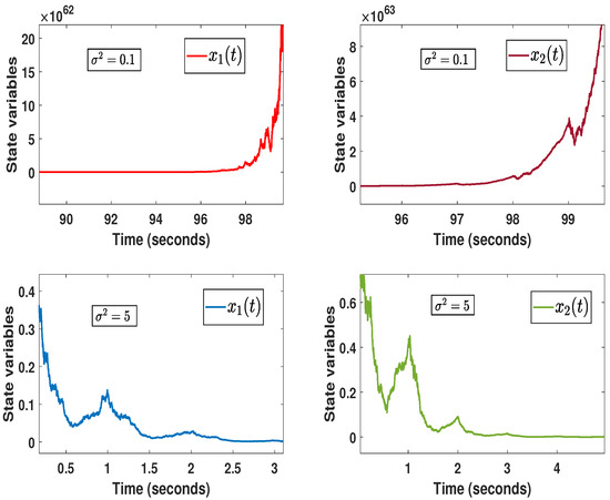
Figure 1. Intermittent Control and Dynamic Parameters.

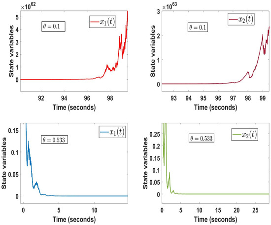
Figure 2. Intermittent Control and Dynamic Parameters.

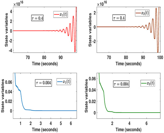
Figure 3. Intermittent Control and Dynamic Parameters.

Example 2.

Consider a two-dimensional system with delays:

$$\begin{array}{c}A=\left(\begin{array}{cc}0.2& 0.1\\ 0.1& 0.2\end{array}\right),B_{11}=\left(\begin{array}{cc}-0.5& 0\\ 0& -0.5\end{array}\right),B_{12}=\left(\begin{array}{cc}0& 0\\ 0& 0\end{array}\right),B_{21}=\left(\begin{array}{cc}0& 0\\ 0& 0\end{array}\right),B_{22}=\left(\begin{array}{cc}-0.5& 0\\ 0& -0.5\end{array}\right)\hfill \\ C_1=\left(\begin{array}{cc}0.1& 0\\ 0& 0.1\end{array}\right),C_2=\left(\begin{array}{cc}0.1& 0\\ 0& 0.1\end{array}\right),Z_{11}=\left(\begin{array}{cc}0.2& 0\\ 0& 0.2\end{array}\right)Z_{12}=\left(\begin{array}{cc}0& 0\\ 0& 0\end{array}\right),Z_{22}=\left(\begin{array}{cc}0.2& 0\\ 0& 0.2\end{array}\right)\hfill \\ Z_1=\left(\begin{array}{cc}2& 0\\ 0& 2\end{array}\right),Z_2=\left(\begin{array}{cc}2& 0\\ 0& 2\end{array}\right),H=\left(\begin{array}{cc}0.5& 0\\ 0& 0.5\end{array}\right).\hfill \end{array}$$

The design of the control functions $u\left(x\right(t-\tau \left)\right)$ are as follows:

$$u\left(x\right)=\left(\begin{array}{c}-4x_1(t-\tau )\\ -4x_2(t-\tau )\end{array}\right).$$

The values of the random term are given in the following matrix:

$$O=\left\{\Psi =\left(\begin{array}{cc}{\delta }_{11}& {\delta }_{12}\\ {\delta }_{12}& {\delta }_{22}\end{array}\right):{\delta }_{11}\in [0.8,1],{\delta }_{12}\in [0.5,0.8],{\delta }_{22}\in [0.8,1]\right\}.$$

Through the MATLAB LMI toolbox, we have:

$$P_{11}=\left(\begin{array}{cc}1.82& 0\\ 0& 1.82\end{array}\right),P_{22}=\left(\begin{array}{cc}1.82& 0\\ 0& 1.82\end{array}\right),Q_{11}=\left(\begin{array}{cc}2.9& 0\\ 0& 2.9\end{array}\right),Q_{22}=\left(\begin{array}{cc}2.9& 0\\ 0& 2.9\end{array}\right),$$

after calculation, it is easy to obtain ${\beta }_1=0.31$, ${\beta }_2=0.35$, ${\beta }_3=0.14$, ${\beta }_4=0.4$, ${\beta }_5=0.56$, $T=0.9$. Substituting the above values into Equation (14), we obtain $\tau =0.0076$. The simulation in Figure 3 clearly shows that the system is stable when the delay $\tau <0.0076$. When the delay $\tau >0.0076$, the system becomes unstable.

6. Conclusions

In this paper, we have investigated stochastic intermittent control strategies based on G-Brownian motion and parameter uncertainties. The key contributions of our work can be summarized as follows: We demonstrated that the system remains stable even under parameter uncertainties by constructing appropriate Lyapunov functions and applying G-expectation theory, addressing a significant challenge in practical applications where parameters cannot always be precisely known. Additionally, we extended the analysis to systems with delays and intermittent control strategies, proving that stability can still be maintained, which is particularly relevant for real-world systems where delays and resource constraints necessitate intermittent control. Future research can build on this work by relaxing some of the assumptions made in this study, such as known system parameters and linear control functions, to enhance the applicability of the methods. Furthermore, implementing and validating the proposed methods in real-world systems, such as industrial processes or networked control systems, would provide valuable insights and confirm their practical effectiveness. Lastly, investigating advanced control strategies, such as adaptive and robust control, in the context of G-Brownian motion and intermittent control could further improve system performance under uncertainty and resource constraints.

References

- Mao, X. Stochastic Differential Equations and Applications, 2nd ed.; Horwood: Chichester, UK, 2007. [Google Scholar]
- Higham, D.; Mao, X.; Stuart, A. Strong convergence of Euler-type methods for nonlinear stochastic differential equations. Siam J. Numer. Anal. 2002, 40, 1041–1063. [Google Scholar] [CrossRef]
- Zhu, Q. Stabilization of stochastic nonlinear delay systems with exogenous disturbances and the event-triggered feedback control. IEEE Trans. Autom. Control 2019, 64, 3764–3771. [Google Scholar] [CrossRef]
- Yin, Z.; Zhu, Q. Stabilization of stochastic highly nonlinear delay systems with neutral term. IEEE Trans. Autom. Control 2023, 68, 2544–2551. [Google Scholar]
- Hao, X.; Zhu, Q.; Xing, Z. Exponential stability of stochastic nonlinear delay systems subject to multiple periodic impulses. IEEE Trans. Autom. Control 2024, 69, 2621–2628. [Google Scholar]
- Lina, F.; Zhu, Q.; Xing, Z. Stability analysis of switched stochastic nonlinear systems with state-dependent delay. IEEE Trans. Autom. Control 2024, 69, 2567–2574. [Google Scholar]
- Hasminskii, R. Stochastic Stability of Differential Equations; Sijthoff and Noordhoff: Groningen, The Netherlands, 1981. [Google Scholar]
- Mao, X. Stochastic stabilization and destabilization. Syst. Control Lett. 1994, 23, 279–290. [Google Scholar] [CrossRef]
- Mao, X.; Yin, G.; Yuan, C. Stabilization and destabilization of hybrid systems stochastic differential equations. Automatica 2007, 43, 264–273. [Google Scholar] [CrossRef]
- Nair, G.; Evans, R. Stabilizability of stochastic linear systems with finite feedback data rates. Siam J. Control Optim. 2004, 43, 413–436. [Google Scholar] [CrossRef]
- Mao, X.; Lam, J.; Huang, L. Stabilisation of hybrid stochastic differential equations by delay feedback control. Syst. Control Lett. 2008, 57, 927–935. [Google Scholar] [CrossRef]
- Mao, X. Almost sure exponential stabilization by discrete-time stochastic feedback control. IEEE Trans. Autom. Control 2016, 61, 1619–1624. [Google Scholar] [CrossRef]
- Deng, F.; Luo, Q.; Mao, X. Stochastic stabilization of hybrid differential equations. Automatica 2012, 48, 2321–2328. [Google Scholar] [CrossRef]
- Yu, K.; Zhai, D.-H.; Liu, G.-P.; Zhao, Y.-B.; Zhao, P. Stability analysis of a class of hybrid stochastic retarded systems under asynchronous switching. IEEE Trans. Autom. Control 2014, 59, 1511–1523. [Google Scholar]
- Lu, Z.; Hu, J.; Mao, X. Stabilisation by delay feedback control for highly nonlinear hybrid stochastic differential equations. Discret. Contin. Dyn.-Syst.-Ser. B 2019, 24, 4099–4116. [Google Scholar] [CrossRef]
- Hu, J.; Liu, W.; Deng, W.; Mao, X. Advances in stabilization of hybrid stochastic differential equations by delay feedback control. Siam J. Control Optim. 2020, 58, 735–754. [Google Scholar] [CrossRef]
- Zong, X.; Wu, F.; Yin, G. Stochastic regularization and stabilization of hybrid functional differential equations. In Proceedings of the IEEE Conference on Decision and Control (CDC), Osaka, Japan, 15–18 December 2015; Volume 54, pp. 1211–1216. [Google Scholar]
- Zhu, Q.; Zhang, Q. Pth moment exponential stabilisation of hybrid stochastic differential equations by feedback controls based on discrete-time state observations with a time delay. IET Control Theory Appl. 2017, 11, 1992–2003. [Google Scholar] [CrossRef]
- Astrom, K.; Wittenmark, B. Computer-Controlled Systems: Theory and Design, 3rd ed.; Prentice Hall: Upper Saddle River, HJ, USA, 1997. [Google Scholar]
- Shevitz, D.; Paden, B. Lyapunov stability theory of nonsmooth systems. IEEE Trans. Autom. Control 1991, 36, 495–500. [Google Scholar]
- Heemels, W.; Donkers, M.; Teel, A. Periodic event-triggered control for linear systems. IEEE Trans. Autom. Control 2013, 58, 847–861. [Google Scholar] [CrossRef]
- Heydari, A. Optimal Switching with Minimum Dwell Time Constraint. J. Frankl. Inst. 2017, 354, 4498–4518. [Google Scholar] [CrossRef]
- Nesic, D.; Teel, A. A framework for stabilization of nonlinear sampled-data systems based on their approximate discrete-time models. IEEE Trans. Autom. Control 2004, 49, 1103–1122. [Google Scholar] [CrossRef]
- Mayne, D.; Rawlings, J.; Rao, C.; Scokaert, P. Constrained model predictive control: Stability and optimality. Automatica 2000, 36, 789–814. [Google Scholar] [CrossRef]
- Chen, C. Robust self-organizing neural-fuzzy control with uncertainty observer for mi-mo nonlinear systems. IEEE Trans. Fuzzy Syst. 2011, 19, 694–706. [Google Scholar] [CrossRef]
- Magdi, S. Passive Control Synthesis for Uncertain Time-delay Systems. In Proceedings of the American Conference on Decision and Control, Tampa, FL, USA, 18 December 1998; IEEE Press: Piscataway, NJ, USA, 1998; Volume 37, pp. 4139–4143. [Google Scholar]
- Iwasaki, T.; Skelton, R. All controllers for the general H∞ control problem: LMI existence conditions and state space formulas. Automatica 1994, 30, 1307–1317. [Google Scholar] [CrossRef]
- Ma, Z.; Yuan, S.; Meng, K.; Mei, S. Mean-square stability of uncertain delayed stochastic systems driven by G-Brownian motion. Mathematics 2023, 11, 2405. [Google Scholar] [CrossRef]
- Peng, S. G-expectation, G-Brownian motion and related stochastic calculus of Itô type. Stoch. Anal. Appl. Abel Symp. 2007, 2, 541–567. [Google Scholar]
- Peng, S. Multi-Dimensional G-Brownian motion and related stochastic calculus under G-Expectation. Stoch. Process. Their Appl. 2008, 118, 2223–2253. [Google Scholar] [CrossRef]
- Ren, Y.; Jia, X.; Hu, L. Exponential stability of solutions to impulsive stochastic differential equations driven by G-Brownian motion. Discret. Contin. Dyn. Syst. B 2017, 20, 2157–2169. [Google Scholar] [CrossRef]
- Zhu, Q.; Huang, T. Stability analysis for a class of stochastic delay nonlinear systems driven by G-Brownian motion. Syst. Control Lett. 2020, 140, 104699. [Google Scholar] [CrossRef]
- Gao, F. Pathwise properties and homeomorphic flows for stochastic differential equations driven by G-Brownian motion. Stoch. Process. Their Appl. 2009, 11, 3356–3382. [Google Scholar] [CrossRef]
- Li, X.; Lin, X.; Lin, Y. Lyapunov-type conditions and stochastic differential equations driven by G-Brownian motion. J. Math. Anal. Appl. 2016, 439, 235–255. [Google Scholar] [CrossRef]
- Liu, Z.; Zhu, Q. Delay feedback control of highly nonlinear neutral stochastic delay differential equations driven by G-Brownian motion. Syst. Control Lett. 2023, 181, 105640. [Google Scholar] [CrossRef]
- Boyd, S.; Ghaoui, L.; Feron, E.; Balakrishnan, V. Linear Matrix Inequalities in System and Control Theory; SIAM: Philadelphia, PA, USA, 1994. [Google Scholar]
Disclaimer/Publisher’s Note: The statements, opinions and data contained in all publications are solely those of the individual author(s) and contributor(s) and not of MDPI and/or the editor(s). MDPI and/or the editor(s) disclaim responsibility for any injury to people or property resulting from any ideas, methods, instructions or products referred to in the content. |
© 2024 by the authors. Licensee MDPI, Basel, Switzerland. This article is an open access article distributed under the terms and conditions of the Creative Commons Attribution (CC BY) license (https://creativecommons.org/licenses/by/4.0/).