A New Reduced-Dimension Iteration Two-Grid Crank–Nicolson Finite-Element Method for Unsaturated Soil Water Flow Problem

Abstract

The main objective of this paper is to reduce the dimensionality of unknown coefficient vectors of finite-element (FE) solutions in two-grid (CN) FE (TGCNFE) format for the nonlinear unsaturated soil water flow problem by using a proper orthogonal decomposition (POD) and to design a new reduced-dimension iteration TGCNFE (RDITGCNFE). For this objective, a new time semi-discrete CN (TSDCN) scheme for the nonlinear unsaturated soil water flow problem is first designed and the existence, stability, and error estimates of TSDCN solutions are demonstrated. Subsequently, a new TGCNFE format for the nonlinear unsaturated soil water flow problem is designed and the existence, unconditional stability, and error estimates of TGCNFE solutions are demonstrated. Next, a new RDITGCNFE format with the same FE basis functions as the TGCNFE format is built by the POD method and the existence, unconditional stability, and error estimates of RDITGCNFE solutions are discussed. Ultimately, the rightness of theory results and the superiority of the RDITGCNFE format are verified by two sets of numerical tests. It is worth noting that the RDITGCNFE format differs completely from all previous reduced-dimension methods, including the authors’ previous works. Therefore, the study of this paper can not only provide a new theoretical method for the dimensionality reduction of numerical models for nonlinear problems but also provide an algorithm implementation technology for the numerical simulation of practical engineering problems.

1. Introduction

With population growth and climate change, global water resources are becoming scarcer and more precious. How to use the limited water resources to ensure the growth of vegetation, especially the growth of crops, without wasting, is an extremely important research topic, which can be attributed to the unsaturated soil water flow problem. In addition, surface and subsurface hydrological processes such as atmospheric precipitation, surface water leakage and deep water rise, plant evapotranspiration, root absorption, and subsurface flow are also attributed to the unsaturated soil water flow problem (see [1,2,3]). Moreover, groundwater movement in homogeneous soil can also be describe by the unsaturated soil water flow equation, and the changes in soil moisture would have a large effect on weather and climate. Therefore, the unsaturated soil water flow problem holds a very important application background.

A significant amount of research (see, e.g., [3,4,5,6]) has shown that the governing equation for the unsaturated soil water flow problem is highly nonlinear because the water flow behavior in porous media of unsaturated soil has high nonlinearity, more precisely, because the relationship between hydraulic conductivity in unsaturated soil and soil moisture is highly nonlinear, which is described by the soil moisture characteristic curve (SMCC). However, SMCCs mostly have two shapes of sigmoidal unimodal and bimodal curves. For the sake of convenience without losing universality, we herein study only the unsaturated soil water flow problem with sigmoidal unimodal SMCCs. Thus, when the horizontal soil water flow can be ignored, the atmospheric general circulation model based on the horizontal resolution (1–5 longitude and latitude) is considered as the one-dimensional unsaturated soil water flow problem, whose water content varies in the soil with depth and time. If the z axis goes straight down and the origin of coordinates lies on the ground, the soil moisture content at point z away from the ground at time t can be denoted by $\theta (z,t)$. Thus, according to on the continuity principle, the Darcy Law, and previous experience, the unsaturated soil water flow problem with sigmoidal unimodal SMCCs can be denoted by the following highly nonlinear partial differential equation (PDE) (see [1,2,3,4,5,6,7,8]):

Problem 1. 

Find $\theta :[0,t_e]\to C^2(\overline{\Omega })$ meeting

$$\begin{array}{ccc}\hfill & & \left\{\begin{array}{c}{\displaystyle {\partial }_t\theta -{\partial }_z(D(\theta ){\partial }_z\theta )+\tilde{K}(\theta )=S_r,z\in \Omega ,t\in (0,t_e),}\hfill \\ {\displaystyle \theta (z,0)={\theta }_0(z),0⩽z⩽Z,}\hfill \\ {\displaystyle \theta (Z,t)=\beta (t),t\in (0,t_e),}\hfill \\ {\displaystyle \theta (0,t)=0,t\in (0,t_e),}\hfill \end{array}\right.\hfill \end{array}$$

(1)

where θ is the unknown moisture content, $t_e$ is a given time upper limit, $\Omega =(0,Z)$ is a bounded interval, Z is the maximum depth of soil, ${\partial }_{\tau }=\partial /\partial \tau$$(\tau =t,z)$, $-S_r$ is the rate of root water absorption, $D(\theta )$ is the soil water diffusion coefficient, $\tilde{K}(\theta )={\partial }_z\widehat{K}(\theta )$, $\widehat{K}(\theta )$ is the soil water conductivity, and $\beta (t)$ and ${\theta }_0(z)$ are the known water content at the lower boundary and initial water content, respectively.

The relationships between the soil water conductivity, $\widehat{K}$, and soil water diffusion coefficient, D, with the moisture content, $\theta$, in Problem 1 are as follows:

$$\begin{array}{c}\hfill {\displaystyle \widehat{K}(\theta )={\tilde{K}}_s{\left(\frac{\theta }{{\theta }_s}\right)}^{2b+3},D(\theta )=b{\tilde{K}}_s{\psi }_s{\theta }_s^{-1}{\left(\frac{\theta }{{\theta }_s}\right)}^{b+2},}\end{array}$$

(2)

where ${\theta }_r⩽\theta (z,t)⩽{\theta }_s,$${\theta }_r$ and ${\theta }_s$ ($0<{\theta }_s⩽1$) stand, respectively, for the known residual and saturated moisture in soil, and the saturated water conductivity, ${\tilde{K}}_s$, soil parameter, b, and saturated soil water potential, ${\psi }_s$, are three known constants. Obviously, $\tilde{K}(\theta )$, ${\displaystyle \mathrm{d}\tilde{K}(\theta )/\mathrm{d}\theta =:{\tilde{K}}^{\prime }(\theta )}$, $D(\theta )$, and ${\displaystyle \mathrm{d}D(\theta )/\mathrm{d}\theta =:D^{\prime }(\theta )}$ are bounded; namely, there are two positive constants, $c_1$ and $c_2$, such that

$$\begin{array}{ccc}\hfill & & {\displaystyle c_1⩽|\tilde{K}(\theta )|,|{\tilde{K}}^{\prime }(\theta )|,|D(\theta )|,|D^{\prime }(\theta )|⩽c_2.}\hfill \end{array}$$

(3)

As mentioned above, the unsaturated soil flow equation has a very wide range of applications. However, because of the strong nonlinearity of the unsaturated soil water flow equation, it is difficult to find its analytical solution, so the best choice is to find its numerical solution by numerical simulation. By lucky coincidence, the numerical simulation for moisture in the unsaturated soil plays an important guiding role in agricultural engineering, atmospheric science, environmental engineering, soil science, and groundwater dynamics. Therefore, it is very important to study the numerical simulation of moisture in unsaturated soil (see [7,8]).

The finite-difference (FD) scheme and finite-element (FE) method are two of the most common numerical ways of solving the unsaturated soil water flow equation. However, the FD scheme is very sensitive to both soil parameters and boundary value conditions. The FE method in [9,10] can deal with the boundary conditions well, but it is very difficult for it to deal with two strong nonlinear terms. In particular, when it is used to solve real-world engineering problems, it contains many unknowns (usually exceeding millions) and is not easy to settle (see, e.g., [11]). Therefore, there are two missions herein. The first mission is to design a new two-grid Crank–Nicolson (CN) FE (TGCNFE) format with the unconditional stability for the unsaturated soil flow equation to simplify calculation and improve accuracy. It is worth noting that the TGCNFE format of the unsaturated soil flow equation herein is not only unconditionally stable but also has second-order time accuracy. Hence it is completely distinct from the monolayer-grid formats in [9,10] and is very novel. The second mission is to use the proper orthogonal decomposition (POD) to lower the dimension of the unknown coefficient vectors of FE solutions in the TGCNFE format for the unsaturated soil flow equation and to design a new reduced-dimension iteration TGCNFE (RDITGCNFE) format to alleviate calculated workload, reduce CPU operating time, and enhance computing efficiency, which is the ultimate mission of this paper.

It is well known that the two-grid FE (TGFE) method is one of the best numerical methods for solving nonlinear PDEs. The method solves a nonlinear FE system of equations on more coarse grids, while solving a linear FE system of equations on fine FE grids with sufficiently high precision. Hence it can simplify computation and enhance calculation efficiency and has been widely used. For example, a TGFE method for semilinear elliptic equations was proposed by Xu in [12], and some TGFE methods for somewhat more complex nonlinear PDEs were developed by Shi’s team in [13,14]. However, to our knowledge, there have been no reports that the TGFE method has been used to deal with the CNFE method for the unsaturated soil flow equation. In particular, the unsaturated soil flow equation with two strongly nonlinear terms, $D(\theta )$ and $\tilde{K}(\theta )$, is far more complex than the nonlinear equations in [12,13,14]. Therefore, no matter the design of the TGCNFE format of the unsaturated soil flow equation or the demonstration of existence and unconditional stability as well as error estimates for the TGCNFE solutions, it faces more difficulties than the previous works. However, the unsaturated soil flow equation has very extensive applications and the TGCNFE solutions have second-order time accuracy and unconditional stability. Hence, it is necessary to study the TGCNFE method for the unsaturated soil flow equation.

A significant amount of numerical simulations (see [15,16,17,18,19,20,21,22,23,24,25,26,27,28,29,30,31,32,33]) have revealed that the POD method plays an important role in lessening the unknowns of numerical models and has been successfully used in various fields, such as fluid mechanics and atmospheric sciences (see [34]), statistics (see [35]), and image recognition and signal processing (see [36]).

Nevertheless, as far as we know, there are no reports that the POD method has been used to reduce the dimensionality of the unknown TGCNFE solution vectors of the unsaturated soil water flow equation. Therefore, we herein design a new RDITGCNFE format by using the POD method to lower the unknown coefficient vectors of TGCNFE solutions while keeping the FE basis functions in the RDITGCNFE format unchanged. Thus, the designed RDITGCNFE format has the same accuracy as the classical TGCNFE format, but it only includes a few unknowns. Therefore, the RDITGCNFE format can greatly lighten the calculated workload, alleviate the accumulation of computation errors, save CPU operating time, and improve the calculation efficiency; see numerical examples in Section 4.

Although some reduced-dimension formats of the unknown coefficient vectors of FE solutions in FE formats with monolayer-grid for linear PDEs have been contributed in [28,29,30,31,32,33], the RDITGCNFE format for the unsaturated soil flow equation with two strongly nonlinear terms in this paper is more complicated than the previous reduced-dimensional FE formats for linear PDEs. Therefore, both the construction of RDITGCNFE format and the demonstration of existence, unconditional stability, and error estimates of the RDITGCNFE solutions are confronted with more difficulties and require more techniques than those in [28,29,30,31,32,33]. However, the RDITGCNFE format for the unsaturated soil water flow equation has second-order time accuracy and unconditional stability, which has higher fidelity than the existing reduced-dimension FE formats, including the reduced-dimensional mixed-FE format with only first-order time accuracy for the unsaturated soil water flow equation in [37]. Hence, it is very valuable to design a RDITGCNFE format for the unsaturated soil water flow equation.

To this end, in Section 2 we first design a new TGCNFE format for the unsaturated soil water flow equation and demonstrate the existence and unconditional stability as well as error estimations of the TGCNFE solutions. Thereafter, in Section 3 we use the POD method to lower the dimension of unknown coefficient vectors of CNFE solutions in the TGCNFE format to establish a new RDITGCNFE format and resort to the matrix theory to demonstrate the existence and unconditional stability, together with error estimations, of the RDITGCNFE solutions. After that, in Section 4 we utilize two sets of numerical tests to verify the effectiveness of the RDITGCNFE format and rightness of our theoretical results. Finally, in Section 5 we generalize the main conclusions of this paper and give some discussions. Thus, the research of this paper can not only provide a new theoretical method for the dimensionality reduction of numerical algorithms of nonlinear problems but also provide an algorithm implementation technique for numerical computations of practical problems.

2. The TGCNFE Method for the Unsaturated Soil Water Flow Equation

2.1. Variational Problem and Time Semi-Discrete CN Scheme

The Sobolev spaces along with norms used herein are traditional (see [38,39]). Let $\mathbb{H}=H_0^1(\Omega )$. For the sake of theoretical analysis, in the following discussion we assume that $\beta (t)=0$. Then, by the Green formula, we can deduce the following variational form:

Problem 2. 

For any $t\in (0,t_e)$, find $\theta \in \mathbb{H}$ meeting

$$\begin{array}{ccc}\hfill & & \left\{\begin{array}{cc}{\displaystyle ({\partial }_t\theta ,\upsilon )+(D(\theta ){\partial }_z\theta ,{\partial }_z\upsilon )+(\tilde{K}(\theta ),\upsilon )=(S_r,\upsilon ),}\hfill & \forall \upsilon \in \mathbb{H},\hfill \\ {\displaystyle \theta (z,0)={\theta }_0(z),}\hfill & z\in \Omega ,\hfill \end{array}\right.\hfill \end{array}$$

(4)

in which $(·,·)$ is an $L^2$ inner product, i.e., $(\vartheta ,\upsilon )={\int }_{\Omega }\vartheta (z)·\upsilon (z)\mathrm{d}z$.

Using the proof method in [10] or the following proof approach of Theorem 1, we can prove the existence and stability of a generalized solution for Problem 2.

To establish the TGCNFE format, we first use the CN method to discretize the time in Problem 2. Therefore, let $K>0$ be an integer, $\Delta t=t_e/K$ be the time-step increment, and ${\theta }^k$ be the approximations of $\theta (z,t)$ at $t_k=n\Delta t$ ($0⩽k⩽K$).

Using an implicit scheme in time to discretize the first equation in Problem 2 yields

$$\begin{array}{ccc}\hfill & & {\displaystyle \frac{1}{\Delta t}({\theta }^k-{\theta }^{k-1},\upsilon )+(D({\theta }^k){\partial }_z{\theta }^k,{\partial }_z\upsilon )+(\tilde{K}({\theta }^k),\upsilon )=(S_r^k,\upsilon ),\forall \upsilon \in \mathbb{H}.}\hfill \end{array}$$

(5)

Using an explicit scheme in time to discretize the first equation in Problem 2 yields

$$\begin{array}{c}\hfill {\displaystyle \frac{1}{\Delta t}({\theta }^k-{\theta }^{k-1},\upsilon )+(D({\theta }^{k-1}){\partial }_z{\theta }^{k-1},{\partial }_z\upsilon )+(\tilde{K}({\theta }^{k-1}),\upsilon )=(S_r^{k-1},\upsilon ),\forall \upsilon \in \mathbb{H}.}\end{array}$$

(6)

By adding (5) and (6), a new time semi-discrete CN (TSDCN) scheme is obtained in the following, which is completely different from all previous schemes:

Problem 3. 

Find ${\left\{{\theta }^k\right\}}_{k=1}^K\subset \mathbb{H}$ meeting

$$\begin{array}{ccc}\hfill & & \left\{\begin{array}{c}{\displaystyle \frac{1}{\Delta t}({\theta }^k-{\theta }^{k-1},\upsilon )+\frac{1}{2}(D({\theta }^k){\partial }_z{\theta }^k+D({\theta }^{k-1}){\partial }_z{\theta }^{k-1},{\partial }_z\upsilon )}\hfill \\ {\displaystyle +\frac{1}{2}(\tilde{K}({\theta }^k)+\tilde{K}({\theta }^{k-1}),\upsilon )=\frac{1}{2}(S_r^k+S_r^{k-1},\upsilon ),\forall \upsilon \in \mathbb{H},1⩽k⩽K,}\hfill \\ {\displaystyle {\theta }^0(z)={\theta }_0(z),z\in \Omega .}\hfill \end{array}\right.\hfill \end{array}$$

(7)

For Problem 3, we have the following results:

Theorem 1. 

Problem 3 has a unique set of TSDCN solutions, ${\left\{{\theta }^k\right\}}_{k=1}^K\subset \mathbb{H}$, meeting the following boundability (i.e., stability):

$$\begin{array}{ccc}\hfill & & {\displaystyle \parallel {\theta }^k{\parallel }_1⩽c(\parallel {\theta }_0{\parallel }_1+\parallel S_r{\parallel }_{0,\infty }),1⩽k⩽K.}\hfill \end{array}$$

(8)

Here, and in the subsequent equations, c is a generical positive constant independent of $\Delta t$. Furthermore, when ${\theta }_0(\mathit{x})$ is smooth enough, the solutions ${\left\{{\theta }^k\right\}}_{k=1}^K$ for Problem 3 satisfies the following error estimates:

$$\begin{array}{ccc}\hfill & & {\displaystyle |\theta (t_k)-{\theta }^k{|}_1⩽c\Delta t^2,1⩽k⩽K,}\hfill \end{array}$$

(9)

in which $\theta (t_k)$$(1⩽k⩽K)$ are the solution $\theta (z,t)$ to Problem 2 at $t=t_k$.

Proof. 

The proof of Theorem 1 consists of the following three parts.

(1) The existence of TSDCN solutions of Problem 3.

For fixing k, we consider the following linearized problem:

Problem 4. 

For the obtained ${\theta }^{k-1}$$(1⩽k⩽K)$, find ${\left\{{\theta }_m^k\right\}}_{m=1}^{\infty }\subset \mathbb{H}$$(1⩽k⩽K)$ meeting

$$\begin{array}{ccc}\hfill & & {\displaystyle ({\theta }_m^k,\upsilon )+\frac{\Delta t}{2}(D({\theta }_{m-1}^k){\partial }_z{\theta }_m^k,{\partial }_z\upsilon )=\frac{\Delta t}{2}(S_r^k+S_r^{k-1},\upsilon )-\frac{\Delta t}{2}(D({\theta }^{k-1}){\partial }_z{\theta }^{k-1},{\partial }_z\upsilon )}\hfill \\ \hfill & & {\displaystyle -\frac{\Delta t}{2}(\tilde{K}({\theta }_{m-1}^k)+\tilde{K}({\theta }^{k-1}),\upsilon ),\forall \upsilon \in \mathbb{H},1⩽k⩽K,m=1,2,\cdots ,}\hfill \end{array}$$

(10)

$$\begin{array}{ccc}\hfill & & {\displaystyle {\theta }_0^1(z)={\theta }_1^0(z)={\theta }^0(z)={\theta }_0(z),z\in \Omega .}\hfill \end{array}$$

(11)

Taking $\vartheta ={\theta }_m^k$ in (10), by (3), the Hölder and Cauchy inequalities, and Lagrange’s mean value theorem of differentiation, we obtain

$$\begin{array}{ccc}\hfill & & {\displaystyle \parallel {\theta }_m^k{\parallel }_0^2+\frac{c_1\Delta t}{2}|{\theta }_m^k{|}_1^2⩽|({\theta }_m^k,{\theta }_m^k)+\frac{\Delta t}{2}(D({\theta }_{m-1}^k){\partial }_z{\theta }_m^k,{\partial }_z{\theta }_m^k)|}\hfill \\ \hfill & & {\displaystyle =|\frac{\Delta t}{2}(\tilde{K}({\theta }_{m-1}^k)+\tilde{K}({\theta }^{k-1})-D({\theta }^{k-1}){\partial }_z{\theta }^{k-1},{\partial }_z{\theta }_m^k)+\frac{\Delta t}{2}(S_r^k+S_r^{k-1},{\theta }_m^k)|}\hfill \\ \hfill & & {\displaystyle ⩽\frac{\Delta t}{2}\underset{\zeta \in \mathbb{H}}{max}|{\tilde{K}}^{\prime }(\zeta )|(\parallel {\theta }_{m-1}^k{\parallel }_0+\parallel {\theta }^{k-1}{\parallel }_0)|{\theta }_m^k{|}_0}\hfill \\ \hfill & & {\displaystyle +\frac{c_2\Delta t}{2}|{\theta }^{k-1}{|}_1|{\theta }_m^k{|}_1+\frac{\Delta t}{2}(\parallel S_r^k{\parallel }_0+\parallel S_r^{k-1}{\parallel }_0)\parallel {\theta }_m^k{\parallel }_0}\hfill \\ \hfill & & {\displaystyle ⩽\frac{1}{2}\parallel {\theta }_m^k{\parallel }_0^2+\frac{c_1\Delta t}{2}|{\theta }_m^k{|}_1^2+c\Delta t^2(\parallel S_r^k{\parallel }_0^2+\parallel S_r^{k-1}{\parallel }_0^2)}\hfill \\ \hfill & & {\displaystyle +c\Delta t(\parallel {\theta }_{m-1}^k{\parallel }_0^2+\parallel {\theta }^{k-1}{\parallel }_0^2+|{\theta }^{k-1}{|}_1^2),m=1,2,\cdots .}\hfill \end{array}$$

(12)

By simplifying (12), we get

$$\begin{array}{ccc}\hfill & & {\displaystyle \parallel {\theta }_m^k{\parallel }_0^2+\Delta t|{\theta }_m^k{|}_1^2⩽c\Delta t^2(\parallel S_r^k{\parallel }_0^2+\parallel S_r^{k-1}{\parallel }_0^2)}\hfill \\ \hfill & & {\displaystyle +c\Delta t(\parallel {\theta }_{m-1}^k{\parallel }_0^2+\parallel {\theta }^{k-1}{\parallel }_0^2+|{\theta }^{k-1}{|}_1^2),m=1,2,\cdots .}\hfill \end{array}$$

(13)

From (13), we conclude that, when $k=1$ and ${\theta }_0(z)=S_r=0$, there holds ${\left\{{\theta }_m^1\right\}}_{m=1}^{\infty }=\left\{0\right\}$; namely, when $k=1$ and ${\theta }_0(z)=S_r=0$, the linearized Problem 4 has only a series of zero solutions. Furthermore, by taking limitation of $m\to \infty$ for the linearized Problem 4, we conclude that, when ${\theta }_0(z)=S_r=0$ and $k=1$, Problem 3 has only a zero solution.

By using recursion or mathematics induction, from (13) we derive that, when ${\theta }_0(z)=S_r=0$, for all $1⩽k⩽K$, ${\left\{{\theta }_m^k\right\}}_{m=1}^{\infty }=\left\{0\right\}$; namely, when ${\theta }_0(z)=S_r=0$, the linearized Problem 4 has only a series of zero solution sequences. Hence, we claim that the linearized Problem 4 has a unique series of solutions, ${\left\{{\theta }_m^k\right\}}_{m=1}^{\infty }\subset \mathbb{H}$ ($1⩽k⩽K$). By using recursion or mathematics induction, from (13) we conclude that the series of solutions, ${\left\{{\theta }_m^k\right\}}_{m=1}^{\infty }\subset \mathbb{H}$ ($1⩽k⩽K$), are bounded. Hence, there exists a positive real $M_0>0$ meeting:

$$\begin{array}{ccc}\hfill & & {\displaystyle |{\theta }_m^k{|}_1⩽M_0(\parallel {\theta }_0{\parallel }_1+\parallel S_r{\parallel }_{0,\infty }),1⩽k⩽K,m=1,2,\cdots .}\hfill \end{array}$$

(14)

By the weak compactness theorem of Hilbert’s space, $H_0^1(\Omega )$ (see (Theorem 6.2, [38])), we claim that the set ${\left\{{\theta }_m^k\right\}}_{m=1}^{\infty }\subset H_0^1(\Omega )$ has a weakly converging subsequence. We may still denote it into ${\left\{{\theta }_m^k\right\}}_{m=1}^{\infty }\subset H_0^1(\Omega )$, meeting $\underset{m\to \infty }{lim}{\theta }_m^k\stackrel{w}{=}{\theta }^k$$(1⩽k⩽K)$.

Taking the limitation of $m\to \infty$ in the linearized Problem 4, by the continuity of the inner product $(·,·)$, the linear operator ${\partial }_z$, $D(·)$, and $\tilde{K}(·)$, we get

$$\begin{array}{ccc}\hfill & & {\displaystyle ({\theta }^k,\upsilon )+\frac{\Delta t}{2}(D({\theta }^k){\partial }_z{\theta }^k,{\partial }_z\upsilon )=(\underset{m\to \infty }{lim}{\theta }_m^k,\upsilon )+\frac{\Delta t}{2}(D(\underset{m\to \infty }{lim}{\theta }_{m-1}^k){\partial }_z\underset{m\to \infty }{lim}{\theta }_m^k,{\partial }_z\upsilon )}\hfill \\ \hfill & & {\displaystyle =-\frac{\Delta t}{2}(\tilde{K}(\underset{m\to \infty }{lim}{\theta }_{m-1}^k)+\tilde{K}({\theta }^{k-1}),\upsilon )-\frac{\Delta t}{2}(D({\theta }^{k-1}){\partial }_z{\theta }^{k-1},{\partial }_z\upsilon )+\frac{\Delta t}{2}(S_r^k+S_r^{k-1},\upsilon )}\hfill \\ \hfill & & {\displaystyle =-\frac{\Delta t}{2}(\tilde{K}({\theta }^k)+\tilde{K}({\theta }^{k-1}),\upsilon )-\frac{\Delta t}{2}(D({\theta }^{k-1}){\partial }_z{\theta }^{k-1},{\partial }_z\upsilon )}\hfill \\ \hfill & & {\displaystyle +\frac{\Delta t}{2}(S_r^k+S_r^{k-1},\upsilon ),\forall \upsilon \in \mathbb{H},1⩽k⩽K.}\hfill \end{array}$$

(15)

This signifies that Problem 4, i.e., Problem 3, has at least one series of solutions, ${\left\{{\theta }^k\right\}}_{k=1}^K$.

If Problem 3 has another series of solutions, ${\left\{{\tilde{\theta }}^k\right\}}_{k=1}^K\subset H_0^1(\Omega )$, it should satisfy the following system of equations:

$$\begin{array}{ccc}\hfill & & \left\{\begin{array}{c}{\displaystyle \frac{1}{\Delta t}({\tilde{\theta }}^k-{\tilde{\theta }}^{k-1},\upsilon )+\frac{1}{2}(D({\tilde{\theta }}^k){\partial }_z{\tilde{\theta }}^k+D({\tilde{\theta }}^{k-1}){\partial }_z{\tilde{\theta }}^{k-1},{\partial }_z\upsilon )}\hfill \\ {\displaystyle +\frac{1}{2}(\tilde{K}({\tilde{\theta }}^k)+\tilde{K}({\tilde{\theta }}^{k-1}),\upsilon )=\frac{1}{2}(S_r^k+S_r^{k-1},\upsilon ),\forall \upsilon \in \mathbb{H},1⩽k⩽K,}\hfill \\ {\displaystyle {\tilde{\theta }}^0(z)={\theta }_0(z),z\in \Omega .}\hfill \end{array}\right.\hfill \end{array}$$

(16)

Setting $E^k={\theta }^k-{\tilde{\theta }}^k$ and subtracting (16) from (7) yields

$$\begin{array}{ccc}\hfill & & {\displaystyle \frac{1}{\Delta t}(E^k-E^{k-1},\upsilon )+\frac{1}{2}(D({\theta }^k){\partial }_z{\theta }^k+D({\theta }^{k-1}){{\partial }_z\theta }^{k-1},{\partial }_z\upsilon )}\hfill \\ \hfill & & {\displaystyle -\frac{1}{2}(D({\tilde{\theta }}^k){\partial }_z{\tilde{\theta }}^k+D({\tilde{\theta }}^{k-1}){\partial }_z{\tilde{\theta }}^{k-1},{\partial }_z\upsilon )+\frac{1}{2}(\tilde{K}({\theta }^k)+\tilde{K}({\theta }^{k-1}),\upsilon )}\hfill \\ \hfill & & {\displaystyle -\frac{1}{2}(\tilde{K}({\tilde{\theta }}^k)+\tilde{K}({\tilde{\theta }}^{k-1}),\upsilon )=0,\forall \vartheta \in \mathbb{H},0⩽k⩽K,}\hfill \end{array}$$

(17)

$$\begin{array}{ccc}\hfill & & {\displaystyle E^0(z)=0,z\in \Omega .}\hfill \end{array}$$

(18)

Taking $\upsilon =E^k-E^{k-1}$ in (17), noting that ${\parallel ·\parallel }_0⩽c{|·|}_1$, by the Hölder and Cauchy inequalities, Green’s formula, and Lagrange’s mean value theorem of differentiation, we obtain

$$\begin{array}{ccc}\hfill & & {\displaystyle 2\parallel E^k-E^{k-1}{\parallel }_0^2+c_1\Delta t(|E^k{|}_1^2-|E^{k-1}{|}_1^2)}\hfill \\ \hfill & & {\displaystyle ⩽|2(E^k-E^{k-1},E^k-E^{k-1})+\Delta t(D({\theta }^k){\partial }_z(E^k+E^{k-1}),{\partial }_z(E^k-E^{k-1}))|}\hfill \\ \hfill & & {\displaystyle =|\Delta t((D({\theta }^k)-(D({\theta }^{k-1})){\partial }_z{E}^{k-1},{\partial }_z(E^k-E^{k-1}))}\hfill \\ \hfill & & {\displaystyle -\Delta t((D({\theta }^k)-D({\tilde{\theta }}^k)){\partial }_z{\tilde{\theta }}^k,{\partial }_z(E^k-E^{k-1}))}\hfill \\ \hfill & & {\displaystyle -(\tilde{K}({\theta }^k)-\tilde{K}({\tilde{\theta }}^k)+\tilde{K}({\theta }^{k-1})-\tilde{K}({\tilde{\theta }}^{k-1}),E^k-E^{k-1})|}\hfill \\ \hfill & & {\displaystyle ⩽\Delta t|D^{\prime }({\xi }_k)|{\tilde{\theta }}^k{|}_{1,\infty }|E^k{|}_1\parallel E^k-E^{k-1}{\parallel }_0+c\Delta t^2|D^{\prime }({\xi }_{k-1})|{\partial }_t{\theta |}_{0,\infty }|E^{k-1}{|}_1{\parallel E^k-E^{k-1}\parallel }_0}\hfill \\ \hfill & & {\displaystyle +\Delta t|{\tilde{K}}^{\prime }({\zeta }_k)|\parallel E^k{\parallel }_0\parallel E^k-E^{k-1}{\parallel }_0+\Delta t|{\tilde{K}}^{\prime }({\zeta }_{k-1})|\parallel E^{k-1}{\parallel }_0{\parallel E^k-E^{k-1}\parallel }_0}\hfill \\ \hfill & & {\displaystyle ⩽\parallel E^k-E^{k-1}{\parallel }_0+c\Delta t^2(|E^k{|}_1^2+|E^{k-1}{|}_1^2),1⩽k⩽K,}\hfill \end{array}$$

(19)

where both ${\xi }_i$ and ${\zeta }_i$ lie between ${\theta }^i$ and ${\tilde{\theta }}^i$ $(i=k,k-1)$. By simplifying (19) we get

$$\begin{array}{ccc}\hfill & & {\displaystyle |E^k{|}_1^2⩽|E^{k-1}{|}_1^2+c\Delta t(|E^k{|}_1^2+|E^{k-1}{|}_1^2),1⩽k⩽K.}\hfill \end{array}$$

(20)

Summing (20) from 1 to k, when $\Delta t$ is small enough meeting $c\Delta t⩽1/2$, by Gronwall’s inequality, we get

$$\begin{array}{ccc}\hfill & & {\displaystyle |E^k{|}_1^2⩽c|E^0{|}_1^2+c\Delta t\sum _{k=0}^{k-1}|E{|}_1^2⩽c{|E^0|}_1^{2}exp(ck\Delta t),1⩽k⩽K.}\hfill \end{array}$$

(21)

By $E^0=0$ and (21), we obtain $E^k=0$, i.e., ${\tilde{\theta }}^k={\theta }^k$ ($1⩽k⩽K$). Thereupon, Problem 3 has a unique series of solutions, ${\left\{{\theta }^k\right\}}_{k=1}^K$.

(2) The stability of TSDCN solutions ${\left\{{\theta }^k\right\}}_{k=1}^K$ for Problem 3.

Taking $\upsilon ={\theta }^k-{\theta }^{k-1}$ in the first equation of (7), and using the Hölder and Cauchy inequalities, Lagrange’s mean value theorem of differentiation, and Green’s formula, when $c_2\Delta t⩽1/2$ and ${\theta }^{k-1}$ is bounded, i.e., $\parallel {\theta }^{k-1}{\parallel }_{1,\infty }⩽c$, we obtain

$$\begin{array}{ccc}\hfill & & {\displaystyle 2\parallel {\theta }^k-{\theta }^{k-1}{\parallel }_0^2+c_1\Delta t(|{\theta }^k{|}_1^2-|{\theta }^{k-1}{|}_1^2)}\hfill \\ \hfill & & {\displaystyle ⩽|2({\theta }^k-{\theta }^{k-1},{\theta }^k-{\theta }^{k-1})+\Delta t(D({\theta }^k){\partial }_z{\theta }^k+D({\theta }^k){\partial }_z{\theta }^{k-1},{\partial }_z({\theta }^k-{\theta }^{k-1}))|}\hfill \\ \hfill & & {\displaystyle =|\Delta t(D({\theta }^k){\partial }_z{\theta }^{k-1}-D({\theta }^{k-1}){\partial }_z{\theta }^{k-1},{\partial }_z({\theta }^k-{\theta }^{k-1}))}\hfill \\ \hfill & & {\displaystyle +\Delta t(S_r^k+S_r^{k-1},{\theta }^k-{\theta }^{k-1})-\Delta t(\tilde{K}({\theta }^k)+\tilde{K}({\theta }^{k-1}),{\theta }^k-{\theta }^{k-1})|}\hfill \\ \hfill & & {\displaystyle ⩽\Delta t\parallel {\theta }^{k-1}{\parallel }_{1,\infty }|D^{\prime }({\tilde{\zeta }}^k)|\parallel {\theta }^k-{\theta }^{k-1}{\parallel }_0{|{\theta }^k-{\theta }^{k-1}|}_1}\hfill \\ \hfill & & {\displaystyle +\Delta t(\parallel S_r^k{\parallel }_0+\parallel S_r^{k-1}{\parallel }_0)\parallel {\theta }^k-{\theta }^{k-1}{\parallel }_0}\hfill \\ \hfill & & {\displaystyle +\Delta t|(|{\tilde{K}}^{\prime }({\tilde{\xi }}^k)\parallel {\theta }^k{\parallel }_0+|{\tilde{K}}^{\prime }({\tilde{\xi }}^{k-1})\parallel {\theta }^{k-1}{\parallel }_0)\parallel {\theta }^k-{\theta }^{k-1}{\parallel }_0}\hfill \\ \hfill & & {\displaystyle ⩽c\Delta t^2(\parallel S_r^k{\parallel }_0^2+\parallel S_r^{k-1}{\parallel }_0^2+|{\theta }^k{|}_1^2+|{\theta }^{k-1}{|}_1^2)+\parallel {\theta }^k-{\theta }^{k-1}{\parallel }_0^2,1⩽k⩽K,}\hfill \end{array}$$

(22)

where ${\tilde{\zeta }}_k$ lies between ${\theta }^k$ and ${\theta }^{k-1}$, and ${\tilde{\xi }}_i$ lies between ${\theta }^i$ and 0 $(i=k-1,k)$. Thus, by simplifying (22) we obtain

$$\begin{array}{ccc}\hfill & & {\displaystyle |{\theta }^k{|}_1^2-|{\theta }^{k-1}{|}_1^2⩽c\Delta t^2(\parallel S_r^k{\parallel }_0^2+\parallel S_r^{k-1}{\parallel }_0^2+|{\theta }^k{|}_1^2+|{\theta }^{k-1}{|}_1^2),1⩽k⩽K.}\hfill \end{array}$$

(23)

Summing (23) from 1 onto k, when $\Delta t$ is small enough such that $c\Delta t⩽1/2$, we obtain

$$\begin{array}{ccc}\hfill & & {\displaystyle |{\theta }^k{|}_1^2⩽c|{\theta }_0{|}_1^2+c\Delta t\sum _{i=0}^{k-1}(\parallel S_r^i{\parallel }_0^2+|{\theta }^i{|}_1^2),1⩽k⩽K.}\hfill \end{array}$$

(24)

Thus, applying Gronwall’s inequality to (24) yields

$$\begin{array}{c}\hfill {\displaystyle |{\theta }^k{|}_1^2⩽c\left(|{\theta }_0{|}_1^2+\Delta t\sum _{i=0}^{k-1}{\parallel S_r^i\parallel }_0^2\right)exp(ck\Delta t)⩽c(|{\theta }_0{|}_1^2+\parallel S_r^i{\parallel }_{0,\infty }^2),1⩽k⩽K.}\end{array}$$

(25)

It follows that (8) holds, namely that the set of solutions, ${\left\{{\theta }^k\right\}}_{k=1}^K$, for Problem 3 is stable.

(3) The error estimates of TSDCN solutions ${\left\{{\theta }^k\right\}}_{k=1}^K$ for Problem 3.

Using Taylor’s formula, we get

$$\begin{array}{ccc}\hfill & & {\displaystyle \theta (t_k)=\theta (t_{k-\frac{1}{2}})+\frac{\Delta t}{2}{\theta }^{\prime }(t_{k-\frac{1}{2}})+\frac{\Delta t^2}{8}{\theta }^{″}(t_{k-\frac{1}{2}})+\frac{\Delta t^3}{48}{\theta }^{‴}({\varsigma }_{1k}),}\hfill \end{array}$$

(26)

$$\begin{array}{ccc}\hfill & & {\displaystyle \theta (t_{k-1})=\theta (t_{k-\frac{1}{2}})-\frac{\Delta t}{2}{\theta }^{\prime }(t_{k-\frac{1}{2}})+\frac{\Delta t^2}{8}{\theta }^{″}(t_{k-\frac{1}{2}})-\frac{\Delta t^3}{48}{\theta }^{‴}({\varsigma }_{2k}),}\hfill \end{array}$$

(27)

$$\begin{array}{ccc}\hfill & & {\displaystyle f(\theta (t_k))=f(\theta (t_{k-\frac{1}{2}}))+[\theta (t_k)-\theta (t_{k-\frac{1}{2}})]f^{\prime }(\theta (t_{k-\frac{1}{2}}))+O{(\theta (t_k)-\theta (t_{k-\frac{1}{2}}))}^2,}\hfill \end{array}$$

(28)

$$\begin{array}{ccc}\hfill & & {\displaystyle f(\theta (t_{k-1}))=f(\theta (t_{k-\frac{1}{2}}))+[\theta (t_{k-1})-\theta (t_{k-\frac{1}{2}})]f^{\prime }(\theta (t_{k-\frac{1}{2}}))}\hfill \\ \hfill & & {\displaystyle +O{(\theta (t_{k-1})-\theta (t_{k-\frac{1}{2}}))}^2,}\hfill \end{array}$$

(29)

where $t_{k-\frac{1}{2}}⩽{\varsigma }_{1k}⩽t_k$ and $t_{k-1}⩽{\varsigma }_{2k}⩽t_{k-\frac{1}{2}}$. It follows that

$$\begin{array}{ccc}\hfill & & {\displaystyle {\theta }^{\prime }(t_{k-\frac{1}{2}})=\frac{\theta (t_k)-\theta (t_{k-1})}{\Delta t}-\frac{\Delta t^2}{24}{\theta }^{‴}({\widehat{\xi }}_k),t_{k-1}⩽{\widehat{\xi }}_k⩽t_{k+1},}\hfill \end{array}$$

(30)

$$\begin{array}{ccc}\hfill & & {\displaystyle \theta (t_{k-\frac{1}{2}})=\frac{\theta (t_k)+\theta (t_{k-1})}{2}-\frac{\Delta t^2}{16}{\theta }^{″}({\widehat{\varsigma }}_k),t_{k-1}⩽{\widehat{\varsigma }}_k⩽t_{k-\frac{1}{2}},}\hfill \end{array}$$

(31)

$$\begin{array}{ccc}\hfill & & {\displaystyle f(\theta (t_{k-\frac{1}{2}}))=\frac{f(\theta (t_k))+f(\theta (t_{k-1}))}{2}-\Delta t^2{R}_f(z,t),}\hfill \end{array}$$

(32)

where $R_f(\mathit{x},t)$ is a bounded function determined by (26)–(29) and $f(·)=D(·)$ or $\tilde{K}(·)$.

Then, subtracting the first equation of (7) from the first equation of (4) after taking $t=t_{k-\frac{1}{2}}$ and setting ${\varrho }^k=\theta (z,t_k)-{\theta }^k$, we get the following error system of equations:

$$\begin{array}{ccc}\hfill & & {\displaystyle \frac{1}{2}(D(\theta (t_{k-\frac{1}{2}})){\partial }_z(\theta (t_k)+\theta (t_{k-1}))-(D({\theta }^k){\partial }_z{\theta }^k+D({\theta }^{k-1}){\partial }_z{\theta }^{k-1}),\upsilon )}\hfill \\ \hfill & & {\displaystyle +\frac{1}{\Delta t}({\varrho }^k-{\varrho }^{k-1},\upsilon )=\frac{\Delta t^2}{24}({\theta }^{‴}({\widehat{\xi }}_k),\upsilon )+\Delta t^2(R_{\tilde{K}}(z,t),\upsilon )}\hfill \\ \hfill & & {\displaystyle -\frac{1}{2}(\tilde{K}(\theta (t_k))-\tilde{K}({\theta }^k)+\tilde{K}(\theta (t_{k-1}))-\tilde{K}({\theta }^{k-1}),\upsilon )),1⩽k⩽K,}\hfill \end{array}$$

(33)

$$\begin{array}{ccc}\hfill & & {\varrho }^0=0.\hfill \end{array}$$

(34)

Taking $\upsilon ={\varrho }^k-{\varrho }^{k-1}$ in (33), by the Hölder and Cauchy inequalities, Green’s formula, Lagrange’s mean value theorem of differentiation, and Taylor’s formula, we obtain

$$\begin{array}{ccc}\hfill & & {\displaystyle 2\parallel {\varrho }^k-{\varrho }^{k-1}{\parallel }_0^2+c_1\Delta t(|{\varrho }^k{|}_1^2-|{\varrho }^{k-1}{\parallel }_1^2)}\hfill \\ \hfill & & {\displaystyle ⩽\left|2({\varrho }^k-{\varrho }^{k-1},{\varrho }^k-{\varrho }^{k-1})+\Delta t(D(\theta (t_{k-\frac{1}{2}})){\partial }_z({\varrho }^k+{\varrho }^{k-1}),{\partial }_z({\varrho }^k-{\varrho }^{k-1}))\right|}\hfill \\ \hfill & & {\displaystyle =\left|\frac{\Delta t}{2}([(D({\theta }^k)+D({\theta }^{k-1})-(D(\theta (t_k))+D(\theta (t_{k-1}))]{\partial }_z({\theta }^k-{\theta }^{k-1}),{\partial }_z({\varrho }^k-{\varrho }^{k-1}))\right.}\hfill \\ \hfill & & {\displaystyle +\frac{\Delta t}{2}((D({\theta }^k)-D({\theta }^{k-1})){\partial }_z({\theta }^k-{\theta }^{k-1}),{\partial }_z({\varrho }^k-{\varrho }^{k-1}))}\hfill \\ \hfill & & {\displaystyle +\Delta t^3(R_D(z,t){\partial }_z({\theta }^k+{\theta }^{k-1}),{\partial }_z({\varrho }^k-{\varrho }^{k-1}))}\hfill \\ \hfill & & {\displaystyle -\Delta t(\tilde{K}(\theta (t_k))-\tilde{K}({\theta }^k)+\tilde{K}(\theta (t_{k-1}))-\tilde{K}({\theta }^{k-1}),{\varrho }^k-{\varrho }^{k-1})}\hfill \\ \hfill & & {\displaystyle \left.+\frac{\Delta t^3}{12}({\theta }^{‴}({\widehat{\xi }}_k),{\varrho }^k-{\varrho }^{k-1})+\Delta t^3(R_{\tilde{K}}(z,t),{\varrho }^k-{\varrho }^{k-1})\right|}\hfill \\ \hfill & & {\displaystyle ⩽c\parallel {\partial }_z{\partial }_t\theta ({\widehat{\varsigma }}_k){\parallel }_{0,\infty }\underset{\upsilon \in \mathbb{H}}{max}|D^{\prime }(\upsilon )|\Delta t^2(|{\varrho }^k{|}_1+|{\varrho }^{k-1}{|}_1)\parallel {\varrho }^k-{\varrho }^{k-1}{\parallel }_0}\hfill \\ \hfill & & {\displaystyle +c\Delta t^3\parallel {\partial }_z{\partial }_t\theta ({\widehat{\varsigma }}_k){\parallel }_{0,\infty }\underset{\upsilon \in \mathbb{H}}{max}|D^{\prime }(\upsilon )|\parallel {\varrho }^k-{\varrho }^{k-1}{)\parallel }_0}\hfill \\ \hfill & & {\displaystyle +c\Delta t\underset{\upsilon \in \mathbb{H}}{max}|{\tilde{K}}^{\prime }(\upsilon )||({\rho }^k+{\varrho }^{k-1},{\varrho }^k-{\varrho }^{k-1})|+c\Delta t^3{\parallel {\varrho }^k-{\varrho }^{k-1}\parallel }_0}\hfill \\ \hfill & & {\displaystyle ⩽\parallel {\varrho }^k-{\varrho }^{k-1}{\parallel }_0+c\Delta t^2(|{\varrho }^k{|}_1^2+|{\varrho }^{k-1}{|}_1^2)+c\Delta t^6,1⩽k⩽K.}\hfill \end{array}$$

(35)

By predigesting (35), we get

$$\begin{array}{ccc}\hfill & & {\displaystyle |{\varrho }^k{|}_1^2-|{\varrho }^{k-1}{|}_1^2⩽c\Delta t^5+c\Delta t(|{\varrho }^k{|}_1^2+|{\varrho }^{k-1}{|}_1^2),1⩽k⩽K.}\hfill \end{array}$$

(36)

Noting that ${\varrho }^0=0$ and summing (36) from 1 to k, when $\Delta t$ is small enough such that $c\Delta t⩽1/2$, by Gronwall’s inequality we obtain

$$\begin{array}{ccc}\hfill & & {\displaystyle |{\varrho }^k{|}_1^2⩽ck\Delta t^5+c\Delta t\sum _{i=0}^{k-1}{|{\varrho }^i|}_1^2⩽ck\Delta t^{5}exp(ck\Delta t)⩽c\Delta t^4,1⩽k⩽K.}\hfill \end{array}$$

(37)

It is deduced from (37) that (9) holds. This finishes the demonstration of Theorem 1. □

2.2. The TGCNFE Format in Functional Form

To build the TGCNFE format, it is necessary to further use the TGFE method to discretize the spatial variables in Problem 3. Toward this end, we hypothesize that ${\Im }_H$ is a coarse grid division formed by quasi-uniform small intervals on $\overline{\Omega }$, and H denotes the maximum interval length in ${\Im }_H$. For the known integer $l⩾1$, ${\mathbb{P}}_l(E)$ denotes the polynomial space with a degree no more than l, defined on the coarse grid element $E\in {\Im }_H$. Then, the FE subspace defined on the coarse grid division ${\Im }_H$ is denoted as follows:

$$\begin{array}{ccc}& & {\displaystyle {\mathbb{H}}_H=\left\{v_H\in C(\overline{\Omega })\cap \mathbb{H}:v_H{|}_E\in {\mathbb{P}}_l(E),\forall E\in {\Im }_H\right\}.}\hfill \end{array}$$

Furthermore, we hypothesize that ${\Im }_h$ is a fine grid division formed by quasi-uniform small intervals on $\overline{\Omega }$, and h represents the maximum interval length in ${\Im }_h$$(h\ll H)$. Similarly, the FE subspace defined on the fine grid division ${\Im }_h$ is denoted as follows:

$$\begin{array}{ccc}& & {\displaystyle {\mathbb{H}}_h=\left\{v_h\in C(\overline{\Omega })\cap \mathbb{H}:v_h{|}_e\in {\mathbb{P}}_l(e),\forall e\in {\Im }_h\right\}.}\hfill \end{array}$$

Thus, the TGCNFE format can be stated as follows.

Problem 5. 

Step 1. Find ${\theta }_H^k\in {\mathbb{H}}_H$$(1⩽k⩽K)$, defined on the coarse grid division ${\Im }_H$, meeting the nonlinear system of the following equations:

$$\begin{array}{c}\hfill \left\{\begin{array}{c}{\displaystyle \frac{1}{\Delta t}({\theta }_H^k-{\theta }_H^{k-1},{\upsilon }_H)+\frac{1}{2}(D({\theta }_H^k){\partial }_z{\theta }_H^k+D({\theta }_H^{k-1}){\partial }_z{\theta }_H^{k-1},{\partial }_z{\upsilon }_H)}\hfill \\ {\displaystyle =\frac{1}{2}(S_r^k+S_r^{k-1},{\upsilon }_H)-\frac{1}{2}(\tilde{K}({\theta }_H^k)+\tilde{K}({\theta }_H^{k-1}),{\upsilon }_H),\forall {\upsilon }_H\in {\mathbb{H}}_H,1⩽k⩽K,}\hfill \\ {\displaystyle {\theta }_H^0(z)=P_H{\theta }_0(z),z\in \Omega .}\hfill \end{array}\right.\end{array}$$

(38)

Step 2. Find ${\theta }_h^k\in {\mathbb{H}}_h$$(1⩽k⩽K)$, defined on the coarse grid division ${\Im }_h$, meeting the linear system of the following equations:

$$\begin{array}{c}\hfill \left\{\begin{array}{c}{\displaystyle ({\theta }_h^k-{\theta }_h^{k-1},{\upsilon }_h)+\frac{\Delta t}{2}(D({\theta }_H^k){\partial }_z{\theta }_h^k+D({\theta }_h^{k-1}){\partial }_z{\theta }_h^{k-1},{\partial }_z{\upsilon }_h)=\frac{\Delta t}{2}(S_r^k+S_r^{k-1},{\upsilon }_h)}\hfill \\ {\displaystyle -\frac{\Delta t}{2}(\tilde{K}({\theta }_H^k)+({\theta }_h^k-{\theta }_H^k){\tilde{K}}^{\prime }({\theta }_H^k)+\tilde{K}({\theta }_h^{k-1}),{\upsilon }_h),\forall {\upsilon }_h\in {\mathbb{H}}_h,1⩽k⩽K,}\hfill \\ {\displaystyle {\theta }_h^0(z)=P_h{\theta }_0(z),z\in \Omega .}\hfill \end{array}\right.\end{array}$$

(39)

The operators $P_{\kappa }:\mathbb{H}\to {\mathbb{H}}_{\kappa }$$(\kappa =H,h)$ in Problem 5 represent two Ritz projections, i.e., for any $q\in \mathbb{H}$, there are two unique $P_{\kappa }q\in {\mathbb{H}}_{\kappa }$, meeting

$$\begin{array}{c}\hfill {\displaystyle ({\partial }_z(q-P_{\kappa }q),{\partial }_z{q}_{\kappa })=0,\forall q_{\kappa }\in {\mathbb{H}}_{\kappa },\kappa =H,h.}\end{array}$$

(40)

Furthermore, the following error estimates hold:

$$\begin{array}{ccc}\hfill & & {\displaystyle |q-P_{\kappa }{q|}_r⩽C{\kappa }^{l+1-r},\forall q\in \mathbb{H}\cap H^{l+1}(\Omega ),\kappa =H,h,r=0,1.}\hfill \end{array}$$

(41)

For Problem 5, we get the following results.

Theorem 2. 

Problem 5 has a unique set of solutions, ${\left\{{\theta }_H^k\right\}}_{k=1}^K\subset {\mathbb{H}}_H$, defined on the coarse grid division ${\Im }_H$, and a unique set of solutions, ${\left\{{\theta }_h^k\right\}}_{k=1}^K\subset {\mathbb{H}}_h$, defined on the fine grid division ${\Im }_h$, respectively, satisfying the following unconditional boundability, i.e., unconditional stability:

$$\begin{array}{ccc}\hfill & & {\displaystyle \parallel {\theta }_H^k{\parallel }_1+\parallel {\theta }_h^k{\parallel }_1⩽c(\parallel {\theta }_0{\parallel }_1+\parallel S_r{\parallel }_{0,\infty }),1⩽k⩽K.}\hfill \end{array}$$

(42)

Here, c, as used subsequently, is also a generical positive constant independent of H, h, and $\Delta t$. Furthermore, when $\Delta t=O(h)=O(H^2)$, the following error estimates hold:

$$\begin{array}{ccc}\hfill & & {\displaystyle \parallel \theta (t_k)-{\theta }_H^k{\parallel }_0+H{|\theta (t_k)-{\theta }_H^k|}_1⩽c(\Delta t^2+H^{l+1}),1⩽k⩽K,}\hfill \end{array}$$

(43)

$$\begin{array}{ccc}& & {\displaystyle \parallel \theta (t_k)-{\theta }_h^k{\parallel }_0+h{|\theta (t_k)-{\theta }_h^k|}_1⩽c(\Delta t^2+h^l+1+H^{l+3}),1⩽k⩽K,}\hfill \end{array}$$

(44)

where $\theta (t_k)$$(1⩽k⩽K)$ are also the solution $\theta (z,t)$ to Problem 2 at $t=t_k$.

Proof. 

Theorem 2 is proven by the following two parts.

(1) The existence and unconditional stability of TGCNFE solutions.

(i) The existence and unconditional stability of CNFE solutions defined on the coarse grid division ${\Im }_H$.

Noting that the system of Equation (38) has the same form as the system of Equation (7), by the same technique as the one proving Theorem 2 we can demonstrate that the system of Equation (38) has a unique set of solutions, ${\left\{{\theta }_H^k\right\}}_{k=1}^K\subset {\mathbb{H}}_H$, meeting

$$\begin{array}{ccc}\hfill & & {\displaystyle |{\theta }_H^k{|}_1⩽c(\parallel {\theta }_0{\parallel }_1+\parallel S_r{\parallel }_{0,\infty }),1⩽k⩽K.}\hfill \end{array}$$

(45)

(ii) The existence and unconditional stability of CNFE solutions defined on the fine grid division ${\Im }_h$.

The linear system (39) is restated as the following problem.

Find ${\theta }_h^k\in {\mathbb{H}}_h$$(1⩽k⩽K)$, meeting the following linear system:

$$\begin{array}{c}\hfill \left\{\begin{array}{c}{\displaystyle ({\theta }_h^k,{\upsilon }_h)+\frac{\Delta t}{2}(D({\theta }_H^k){\partial }_z{\theta }_h^k,{\partial }_z{\upsilon }_h)+\frac{\Delta t}{2}({\theta }_h^k{\tilde{K}}^{\prime }({\theta }_H^k),{\upsilon }_h)}\hfill \\ {\displaystyle =({\theta }_h^{k-1},{\upsilon }_h)-\frac{\Delta t}{2}(D({\theta }_h^{k-1}){\partial }_z{\theta }_h^{k-1},{\partial }_z{\upsilon }_h)-\frac{\Delta t}{2}(\tilde{K}({\theta }_H^k)+\tilde{K}({\theta }_h^{k-1}),{\upsilon }_h)}\hfill \\ {\displaystyle +\frac{\Delta t}{2}({\theta }_H^k{\tilde{K}}^{\prime }({\theta }_H^k),{\upsilon }_h)+\frac{\Delta t}{2}(S_r^k+S_r^{k-1},{\upsilon }_h),\forall {\upsilon }_h\in {\mathbb{H}}_h,1⩽k⩽K,}\hfill \\ {\displaystyle {\theta }_h^0(z)=P_h{\theta }_0(z),z\in \Omega .}\hfill \end{array}\right.\end{array}$$

(46)

Let $A({\theta }_h^k,{\upsilon }_h)=({\theta }_h^k,{\upsilon }_h)+\frac{\Delta t}{2}(D({\theta }_H^k){\partial }_z{\theta }_h^k,{\partial }_z{\upsilon }_h)+\frac{\Delta t}{2}({\tilde{K}}^{\prime }({\theta }_H^k){\theta }_h^k,{\upsilon }_h)$ and $F({\upsilon }_h)=\frac{\Delta t}{2}(S_r^k$$+S_r^{k-1},{\upsilon }_h)-\frac{\Delta t}{2}(D({\theta }_h^{k-1}){\partial }_z{\theta }_h^{k-1},{\partial }_z{\upsilon }_h)-\frac{\Delta t}{2}(\tilde{K}({\theta }_H^k)+\tilde{K}({\theta }_h^{k-1})-{\tilde{K}}^{\prime }({\theta }_H^k){\theta }_H^k,{\upsilon }_h)+({\theta }_h^{k-1},{\upsilon }_h).$ Thus, the system of Equation (46) can be rewritten as follows.

Find ${\theta }_h^k\in {\mathbb{H}}_h$$(1⩽k⩽K)$, meeting the following linear system:

$$\begin{array}{ccc}\hfill & & \left\{\begin{array}{c}{\displaystyle A({\theta }_h^k,{\upsilon }_h)=F({\upsilon }_h),\forall {\upsilon }_h\in {\mathbb{H}}_h,1⩽k⩽K,}\hfill \\ {\displaystyle {\theta }_h^0(z)=P_h{\theta }_0(z),z\in \Omega .}\hfill \end{array}\right.\hfill \end{array}$$

(47)

When $\Delta t$ is sufficiently small, meeting ${\displaystyle c_2\Delta t{\parallel {\tilde{K}}^{\prime }\parallel }_{0,\infty }<1}$, by (3), we get

$$\begin{array}{ccc}\hfill & & {\displaystyle A({\theta }_h^k,{\theta }_h^k)=({\theta }_h^k,{\theta }_h^k)+\frac{\Delta t}{2}(D({\theta }_H^k){\partial }_z{\theta }_h^k,{\partial }_z{\theta }_h^k)+\frac{\Delta t}{2}({\tilde{K}}^{\prime }({\theta }_H^k){\theta }_h^k,{\theta }_h^k)}\hfill \\ \hfill & & {\displaystyle ⩾\left(1-\frac{c_2\Delta t{\parallel {\tilde{K}}^{\prime }\parallel }_{0,\infty }}{2}\right)\parallel {\theta }_h^k{\parallel }_0^2+\frac{c_1\Delta t}{2}|{\theta }_h^k{|}_1^2⩾{\alpha }_0{\parallel {\theta }_h^k\parallel }_1^2,\forall {\theta }_h^k\in {\mathbb{H}}_h,}\hfill \end{array}$$

(48)

where ${\displaystyle {\alpha }_0=min\{c_1\Delta t/2,1-c_2\Delta t\parallel {\tilde{K}}^{\prime }{\parallel }_{0,\infty }/2\}>0}$. Hence, $A(·,·)$ is positive definite in ${\mathbb{H}}_h$. It is obvious that $A(·,·)$ is a bounded bilinear form in ${\mathbb{H}}_h\times {\mathbb{H}}_h$ and $F(·)$ is a bounded linear form in ${\mathbb{H}}_h$ for the given ${\theta }_H^k$ and ${\theta }_h^{k-1}$. Hence, by the Lax–Milgram Theorem (see Theorem 1.15 [38]) we assert that the system of Equation (46), namely Step 2 in Problem 5, has a unique set of solutions, ${\left\{{\theta }_h^k\right\}}_{k=1}^K\subset {\mathbb{H}}_h$ meeting

$$\begin{array}{ccc}\hfill & & {\displaystyle \parallel {\theta }_h^k{\parallel }_1⩽c(\parallel {\theta }_0{\parallel }_1+\parallel S_r{\parallel }_{0,\infty }),1⩽k⩽K.}\hfill \end{array}$$

(49)

This signifies that the set of solutions, ${\left\{{\theta }_h^k\right\}}_{k=1}^K\subset {\mathbb{H}}_h$, defined on the fine grid division ${\Im }_h$ is unconditionally bounded; namely, it is unconditionally stable.

(2) The error estimates of TGCNFE solutions to Problem 5.

(a) The error estimates of solutions ${\left\{{\theta }_H^k\right\}}_{k=1}^K$ to Problem 5 defined on the coarse grid division ${\Im }_H$.

Subtracting the system of Equation (38) from the system of Equation (7), taking $\upsilon ={\upsilon }_H$ and setting $E_H^k={\theta }^k-{\theta }_H^k$, ${\rho }_H^k={\theta }^k-P_H{\theta }^k$, and ${\omega }_H^k=P_H{\theta }^k-{\theta }_H^k$, we get

$$\begin{array}{ccc}\hfill & & {\displaystyle \frac{1}{\Delta t}(E_H^k-E_H^{k-1},{\upsilon }_H)+\frac{1}{2}(D({\theta }^k){\partial }_z{\theta }^k+D({\theta }^{k-1}){\partial }_z{\theta }^{k-1}),{\partial }_z{\upsilon }_H)}\hfill \\ \hfill & & {\displaystyle -\frac{1}{2}(D({\theta }_H^k){\partial }_z{\theta }_H^k+D({\theta }_H^{k-1}){\partial }_z{\theta }_H^{k-1}),{\partial }_z{\upsilon }_H)}\hfill \\ \hfill & & {\displaystyle =-\frac{1}{2}(\tilde{K}({\theta }^k)-\tilde{K}({\theta }_H^k)+\tilde{K}({\theta }^{k-1})-\tilde{K}({\theta }_H^{k-1}),{\upsilon }_H),\forall {\upsilon }_H\in {\mathbb{H}}_H,1⩽k⩽K,}\hfill \end{array}$$

(50)

$$\begin{array}{ccc}\hfill & & {\displaystyle E_H^0={\theta }_0(z)-P_H{\theta }_0(z),z\in \Omega .}\hfill \end{array}$$

(51)

By (50), (40), the first equation of (39), Taylor’s formula, Lagrange’s mean value theorem of differentiation, and the Hölder and Cauchy inequalities, when $\Delta t=O(H^2)$, noting that $|{\rho }_H^k-{\rho }_H^k{|}_s={|({\theta }^k-{\theta }^{k-1})-P_H({\theta }^k-{\theta }^{k-1})|}_s⩽c\Delta t{H}^{l+1-s}$$(s=0,1)$, from (41) we get

$$\begin{array}{ccc}\hfill & & {\displaystyle \frac{1}{\Delta t}\parallel E_H^k-E_H^{k-1}{\parallel }_0^2+\frac{c_1}{2}(|E_H^k{|}_1^2-|E_H^{k-1}{|}_1^2)}\hfill \\ \hfill & & {\displaystyle ⩽\frac{1}{\Delta t}(E_H^k-E_H^{k-1},E_H^k-E_H^{k-1})+\frac{1}{2}(D({\theta }^k){\partial }_z(E_H^k+E_H^{k-1}),{\partial }_z(E_H^k-E_H^{k-1}))}\hfill \\ \hfill & & {\displaystyle =\frac{1}{\Delta t}(E_H^k-E_H^{k-1},{\rho }_H^k-{\rho }_H^{k-1})+\frac{1}{2}(D({\theta }^k){\partial }_z(E_H^k+E_H^{k-1}),{\partial }_z({\rho }_H^k-{\rho }_H^{k-1}))}\hfill \\ \hfill & & {\displaystyle +\frac{1}{\Delta t}(E_H^k-E_H^{k-1},{\omega }_H^k-{\omega }_H^{k-1})+\frac{1}{2}(D({\theta }^k){\partial }_z(E_H^k+E_H^{k-1}),{\partial }_z({\omega }_H^k-{\omega }_H^{k-1}))}\hfill \\ \hfill & & {\displaystyle =\frac{1}{\Delta t}(E_H^k-E_H^{k-1},{\rho }_H^k-{\rho }_H^{k-1})+\frac{1}{2}(D({\theta }^k){\partial }_z(E_H^k+E_H^{k-1}),{\partial }_z({\rho }_H^k-{\rho }_H^{k-1}))}\hfill \\ \hfill & & {\displaystyle +\frac{1}{\Delta t}(E_H^k-E_H^{k-1},{\omega }_H^k-{\omega }_H^{k-1})+\frac{1}{2}(D({\theta }^k){\partial }_z{\theta }^k+D({\theta }^{k-1}){\partial }_z{\theta }^{k-1}),{\partial }_z({\omega }_H^k-{\omega }_H^{k-1}))}\hfill \\ \hfill & & {\displaystyle -\frac{1}{2}(D({\theta }_H^k){\partial }_z{\theta }_H^k+D({\theta }_H^{k-1}){\partial }_z{\theta }_H^{k-1},{\partial }_z({\omega }_H^k-{\omega }_H^{k-1}))}\hfill \\ \hfill & & {\displaystyle +\frac{1}{2}((D({\theta }^k)-D({\theta }^{k-1})){\partial }_z{\theta }^{k-1}+(D({\theta }_H^k)-D({\theta }^k)){\partial }_z{\theta }_H^k,{\partial }_z({\omega }_H^k-{\omega }_H^{k-1}))}\hfill \\ \hfill & & {\displaystyle +\frac{1}{2}((D({\theta }_H^{k-1})-D({\theta }^k)){\partial }_z{\theta }_H^{k-1},{\partial }_z({\omega }_H^k-{\omega }_H^{k-1}))}\hfill \\ \hfill & & {\displaystyle =\frac{1}{\Delta t}(E_H^k-E_H^{k-1},{\rho }_H^k-{\rho }_H^{k-1})+\frac{1}{2}(D({\theta }^k){\partial }_z(E_H^k+E_H^{k-1}),{\partial }_z({\rho }_H^k-{\rho }_H^{k-1}))}\hfill \\ \hfill & & {\displaystyle +\frac{1}{2}((D({\theta }^k)-D({\theta }^{k-1})){\partial }_z{E}_H^{k-1}+(D({\theta }^k)-D({\theta }_H^k)){\partial }_z{\theta }_H^k,{\partial }_z({\omega }_H^k-{\omega }_H^{k-1}))}\hfill \\ \hfill & & {\displaystyle +\frac{1}{2}((D({\theta }^{k-1})-D({\theta }_H^{k-1})){\partial }_z{\theta }_H^{k-1},{\partial }_z(E_H^k-E_H^{k-1}-{\rho }_H^k+{\rho }_H^{k-1}))}\hfill \\ \hfill & & {\displaystyle -\frac{1}{2}(\tilde{K}({\theta }^k)-\tilde{K}({\theta }_H^k)+\tilde{K}({\theta }^{k-1})-\tilde{K}({\theta }_H^{k-1}),E_H^k-E_H^{k-1}-{\rho }_H^k+{\rho }_H^{k-1})}\hfill \\ \hfill & & {\displaystyle ⩽\frac{1}{4\Delta t}\parallel E_H^k-E_H^{k-1}{\parallel }_0^2+\frac{c}{4\Delta t}\parallel {\rho }_H^k-{\rho }_H^{k-1}{\parallel }_0^2+\frac{c_1}{2}{|{\rho }_H^k-{\rho }_H^{k-1}|}_1^2}\hfill \\ \hfill & & {\displaystyle +\Delta t\underset{{\upsilon }_H\in {\mathbb{H}}_H}{max}|D^{\prime }({\upsilon }_H)||E_H^{k-1}{|}_1{|E_H^k-E_H^{k-1}-{\rho }_H^k+{\rho }_H^{k-1}|}_1}\hfill \\ \hfill & & {\displaystyle +\underset{{\upsilon }_H\in {\mathbb{H}}_H}{max}|D^{\prime }({\upsilon }_H)||{\theta }_H^{k-1}{|}_{1,\infty }|E_H^k{|}_1{\parallel E_H^k-E_H^{k-1}-{\rho }_H^k+{\rho }_H^{k-1}\parallel }_0}\hfill \\ \hfill & & {\displaystyle +\underset{{\upsilon }_H\in {\mathbb{H}}_H}{max}|D^{\prime }({\upsilon }_H)||{\theta }_H^{k-1}{|}_{1,\infty }|E_H^{k-1}{|}_1{\parallel E_H^k-E_H^{k-1}-{\rho }_H^k+{\rho }_H^{k-1}\parallel }_0}\hfill \\ \hfill & & {\displaystyle +\underset{{\upsilon }_H\in {\mathbb{H}}_H}{max}|{\tilde{K}}^{\prime }({\upsilon }_H)|(\parallel E_H^k{\parallel }_0+\parallel E_H^{k-1}{\parallel }_0)\parallel E_H^k-E_H^{k-1}-{\rho }_H^k+{\rho }_H^{k-1}{\parallel }_0}\hfill \\ \hfill & & {\displaystyle ⩽\frac{1}{2\Delta t}\parallel E_H^k-E_H^{k-1}{\parallel }_0^2+c\Delta t(|E_H^k{|}_1^2+|E_H^{k-1}{|}_1^2)+c\Delta t{H}^{2l},1⩽k⩽K.}\hfill \end{array}$$

(52)

By simplifying (52), we get

$$\begin{array}{ccc}\hfill & & {\displaystyle |E_H^k{|}_1^2 - |E_H^{k-1}{|}_1^2⩽c\Delta t(|E_H^k{|}_1^2 + |E_H^{k-1}{|}_1^2) + c\Delta t{H}^{2l},1⩽k⩽K.}\hfill \end{array}$$

(53)

Summating (53) from 1 to k and using (41), when $\Delta t$ is small enough, such that $c\Delta t⩽1/2$, we get

$$\begin{array}{c}\hfill {\displaystyle |E_H^k{|}_1^2⩽c|E_H^0{|}_1^2+ck\Delta t{H}^{2l}+c\Delta t\sum _{i=0}^{k-1}|E_H^i{|}_1^2⩽c{H}^{2l}+c\Delta t\sum _{i=0}^{k-1}{|E_H^i|}_1^2,1⩽k⩽K.}\end{array}$$

(54)

Applying Gronwall’s inequality to (54) yields

$$\begin{array}{c}\hfill {\displaystyle |E_H^k{|}_1^2⩽c{H}^{2l}exp(ck\Delta t^2)⩽c{H}^{2l},1⩽k⩽K.}\end{array}$$

(55)

Thus, by Nitsche’s skill (see Theorem 1.38 or Remark 3.1 [38]) and the inverse estimation theorem (see Corollary 1.24 [38]) as well as (55), we easily get the following error estimates:

$$\begin{array}{ccc}\hfill & & {\displaystyle \parallel {\theta }^k-{\theta }_H^k{\parallel }_0+H{|{\theta }^k-{\theta }_H^k|}_1⩽c{H}^{l+1},1⩽k⩽K.}\hfill \end{array}$$

(56)

Combining (56) with Theorem 1 obtains (43).

(b) The error estimates of solutions ${\theta }_h^k$$(1⩽k⩽K)$ to Problem 5, defined on the fine grid division ${\Im }_h$.

Subtracting the system of Equation (39) from the system of Equation (7), taking $\upsilon ={\upsilon }_h$ and setting $E_h^k={\theta }^k-{\theta }_h^k$, ${\rho }_h^k={\theta }^k-P_h{\theta }^k$, and ${\omega }_h^k=P_h{\theta }^k-{\theta }_h^k$, we attain

$$\begin{array}{ccc}\hfill & & {\displaystyle \frac{1}{\Delta t}(E_h^k-E_h^{k-1},{\upsilon }_h)+\frac{1}{2}(D({\theta }^k){\partial }_z{\theta }^k+D({\theta }^{k-1}){\partial }_z{\theta }^{k-1},{\upsilon }_h)}\hfill \\ \hfill & & {\displaystyle +\frac{1}{2}(\tilde{K}({\theta }^k)-\tilde{K}({\theta }_H^k)+\tilde{K}({\theta }^{k-1})-\tilde{K}({\theta }_h^{k-1})-{\tilde{K}}^{\prime }({\theta }_H^k)({\theta }_h^k-{\theta }_H^k),{\upsilon }_h)}\hfill \\ \hfill & & {\displaystyle -\frac{\Delta t}{2}(D({\theta }_H^k){\partial }_z{\theta }_h^k+D({\theta }_h^{k-1}){\partial }_z{\theta }_h^{k-1},{\partial }_z{\upsilon }_h)=0,\forall {\upsilon }_h\in {\mathbb{H}}_h,1⩽k⩽K,}\hfill \end{array}$$

(57)

$$\begin{array}{ccc}\hfill & & {\displaystyle E_h^0={\theta }_0(z)-P_h{\theta }_0(z),z\in \Omega .}\hfill \end{array}$$

(58)

By (57), (40), Taylor’s formula, Lagrange’s mean value theorem of differentiation, the Hölder and Cauchy inequalities, and (43) or (56), when $\Delta t=O(h)=O(H^2)$, noting that both ${\theta }_h^k$ and ${\theta }_H^k$ are bounded, and $|{\rho }_h^k-{\rho }_h^k{|}_s={|({\theta }^k-{\theta }^{k-1})-P_h({\theta }^k-{\theta }^{k-1})|}_s⩽c\Delta t{h}^{l+1-s}$$(s=0,1)$, we attain

$$\begin{array}{ccc}\hfill & & {\displaystyle \frac{1}{\Delta t}\parallel E_h^k-E_h^{k-1}{\parallel }_0^2+\frac{c_1}{2}(|E_h^k{|}_1^2-|E_h^{k-1}{|}_1^2)}\hfill \\ \hfill & & {\displaystyle ⩽\left|{\displaystyle \frac{1}{\Delta t}(E_h^k-E_h^{k-1},{\rho }_h^k-{\rho }_h^{k-1})+\frac{1}{\Delta t}(E_h^k-E_h^{k-1}),{\omega }_h^k-{\omega }_h^{k-1})}\right.}\hfill \\ \hfill & & {\displaystyle +\frac{1}{2}(D({\theta }^k){\partial }_z(E_h^k+E_h^{k-1}),{\partial }_z({\rho }_h^k-{\rho }_h^{k-1}))+\frac{1}{2}(D({\theta }^k){\partial }_z(E_h^k+E_h^{k-1}),{\partial }_z({\omega }_h^k-{\omega }_h^{k-1}))}\hfill \\ \hfill & & {\displaystyle +\frac{1}{2}(D({\theta }^k){\partial }_z{\theta }^k-D({\Theta }_H^k){\partial }_z{\theta }_h^k+D({\theta }^{k-1}){\partial }_z{\theta }^{k-1}-D({\theta }_h^{k-1}){\partial }_z{\theta }_h^{k-1},{\partial }_z({\omega }_h^k-{\omega }_h^{k-1}))}\hfill \\ \hfill & & {\displaystyle \left.-\frac{1}{2}(D({\theta }^k){\partial }_z{\theta }^k-D({\theta }_H^k){\partial }_z{\theta }_h^k+D({\theta }^{k-1}){\partial }_z{\theta }^{k-1}-D({\theta }_h^{k-1}){\partial }_z{\theta }_h^{k-1},{\partial }_z({\omega }_h^k-{\omega }_h^{k-1}))\right|}\hfill \\ \hfill & & {\displaystyle =\left|{\displaystyle \frac{1}{\Delta t}(E_h^k-E_h^{k-1},{\rho }_h^k-{\rho }_h^{k-1})+\frac{1}{2}(D({\theta }^k){\partial }_z(E_h^k+E_h^{k-1}),{\partial }_z({\rho }_h^k-{\rho }_h^{k-1}))}\right.}\hfill \\ \hfill & & {\displaystyle +\frac{1}{2}(D({\theta }^k){\partial }_z(E_h^k+E_h^{k-1}),{\partial }_z({\omega }_h^k-{\omega }_h^{k-1}))}\hfill \\ \hfill & & {\displaystyle -\frac{1}{2}(D({\theta }^k){\partial }_z{\theta }^k-D({\theta }_H^k){\partial }_z{\theta }_h^k+D({\theta }^{k-1}){\partial }_z{\theta }^{k-1}-D({\theta }_h^{k-1}){\partial }_z{\theta }_h^{k-1},{\partial }_z({\omega }_h^k-{\omega }_h^{k-1}))}\hfill \\ \hfill & & {\displaystyle \left.-\frac{1}{2}(\tilde{K}({\theta }^k)-\tilde{K}({\theta }_H^k)+\tilde{K}({\theta }^{k-1})-\tilde{K}({\theta }_h^{k-1})-{\tilde{K}}^{\prime }({\theta }_H^k)({\theta }_h^k-{\theta }_H^k),{\omega }_h^k-{\omega }_h^{k-1})\right|}\hfill \\ \hfill & & {\displaystyle =\left|{\displaystyle \frac{1}{\Delta t}(E_h^k-E_h^{k-1},{\rho }_h^k-{\rho }_h^{k-1})+\frac{1}{2}(D({\theta }^k){\partial }_z(E_h^k+E_h^{k-1}),{\partial }_z({\rho }_h^k-{\rho }_h^{k-1}))}\right.}\hfill \\ \hfill & & {\displaystyle +\frac{1}{2}((D({\theta }^k)-D({\theta }^{k-1})){\partial }_z{E}_h^{k-1},{\partial }_z({\omega }_h^k-{\omega }_h^{k-1}))}\hfill \\ \hfill & & {\displaystyle -\frac{1}{2}((D({\theta }^k)-D({\theta }_H^k)){\partial }_z{\theta }_h^k+(D({\theta }^{k-1})-D({\theta }_h^{k-1})){\partial }_z{\theta }_h^{k-1},{\partial }_z({\omega }_h^k-{\omega }_h^{k-1}))}\hfill \\ \hfill & & {\displaystyle \left.-\frac{1}{2}(\tilde{K}({\theta }^k)-\tilde{K}({\theta }_H^k)+\tilde{K}({\theta }^{k-1})-\tilde{K}({\theta }_h^{k-1})-{\tilde{K}}^{\prime }({\theta }_H^k)({\theta }_h^k-{\theta }_H^k),{\omega }_h^k-{\omega }_h^{k-1})\right|}\hfill \\ \hfill & & {\displaystyle ⩽\frac{1}{4\Delta t}\parallel E_h^k-E_h^{k-1}{\parallel }_0^2+\frac{1}{\Delta t}\parallel {\rho }_h^k-{\rho }_h^{k-1}{\parallel }_0^2+\frac{c_2}{2}|{\rho }_h^k-{\rho }_h^{k-1}{|}_1{|{\rho }_h^k+{\rho }_h^{k-1}|}_1}\hfill \\ \hfill & & {\displaystyle +c\Delta t\parallel D^{\prime }{\parallel }_{0,\infty }(|E_h^{k-1}{|}_1^2+|E_h^k-E_h^{k-1}{|}_1^2+|{\rho }_h^k-{\rho }_h^{k-1}{|}_1^2)}\hfill \\ \hfill & & {\displaystyle +c\parallel D^{\prime }{\parallel }_{0,\infty }max\{|{\theta }_h^k{|}_{1,\infty },|{\theta }_h^{k-1}{|}_{1,\infty }\}(|E_H^k{|}_1+|E_h^{k-1}{|}_1)\parallel {\omega }_h^k-{\omega }_h^{k-1}{\parallel }_0}\hfill \\ \hfill & & {\displaystyle +c\parallel {\tilde{K}}^{\prime }{\parallel }_{0,\infty }(\parallel {\theta }^k-{\theta }_H^k{\parallel }_0+\parallel E_h^k{\parallel }_0+\parallel E_h^{k-1}{\parallel }_0)\parallel {\omega }_h^k-{\omega }_h^{k-1}{\parallel }_0}\hfill \\ \hfill & & {\displaystyle ⩽\frac{1}{2\Delta t}\parallel E_h^k-E_h^{k-1}{\parallel }_0^2+c\Delta t(|E_h^k{|}_1^2+|E_h^{k-1}{|}_1^2)+c\Delta t{H}^{2l+2}+c\Delta t{h}^{2l},1⩽k⩽K.}\hfill \end{array}$$

(59)

Thus, from (59) we obtain

$$\begin{array}{c}\hfill {\displaystyle |E_h^k{|}_1^2-|E_h^{k-1}{|}_1^2⩽c\Delta t(|E_h^{k-1}{|}_1^2+|E_h^k{|}_1^2)+c\Delta t{H}^{2l+2}+c\Delta t{h}^{2l},1⩽k⩽K.}\end{array}$$

(60)

Summing (60) from 1 to k, when $\Delta t$ is small enough, meeting $c\Delta t⩽1/2$, by Gronwall’s inequality we get

$$\begin{array}{ccc}\hfill & & {\displaystyle |E_h^k{|}_1^2⩽c|E_h^0{|}_1^2+ck\Delta t{H}^{2l+2}+ck\Delta t{h}^{2l}+c\Delta t\sum _{k=1}^{k-1}{|E_h^k|}_1^2}\hfill \\ \hfill & & {\displaystyle ⩽c(h^{2l}+H^{2l+2})exp(ck\Delta t)⩽c(h^{2l}+H^{2l+2}),1⩽k⩽K.}\hfill \end{array}$$

(61)

By Nitsche’s skill and the inverse estimation theorem as well as (61), we easily obtain the following error estimates:

$$\begin{array}{c}\hfill {\displaystyle \parallel {\theta }^k-{\theta }_h^k{\parallel }_0+h|{\theta }^k-{\theta }_h^k{|}_1=\parallel E_h^k{\parallel }_0+h{|E_h^k|}_1⩽c(h^{l+1}+H^{l+3}),1⩽k⩽K.}\end{array}$$

(62)

Thus, the inequality (44) is obtained by combining (62) with Theorem 1. This completes the demonstration of Theorem 2. □

Remark 1. 

Theorem 2 shows that the theoretical errors of TGCNFE solutions reach optimal order, and they are unconditionally stable since $\Delta t$ has no relationship with h and H in the proof of stability.

2.3. The TGCNFE Format in Matrix Form

To build the RDITGCNFE format, it is necessary to rewrite the TGCNFE format in functional form into matrix format. Hence, we set that ${\left\{{\eta }_i\right\}}_{i=1}^{M_H}$$\subset {\mathbb{H}}_H$ and ${\left\{{\tilde{\eta }}_j\right\}}_{j=1}^{M_h}$$\subset {\mathbb{H}}_h$ are two series of orthonormal basis functions under the $L^2$ inner product, i.e., they meet $({\eta }_i,{\eta }_{\ell })=\left\{\begin{array}{cc}1,\hfill & i=\ell \hfill \\ 0,\hfill & i\ne \ell \hfill \end{array}\right.$ and $({\tilde{\eta }}_j,{\tilde{\eta }}_m)=\left\{\begin{array}{cc}1,\hfill & j=m\hfill \\ 0,\hfill & j\ne m\hfill \end{array}\right.$, which can be obtained by the orthonormal technique in Section 1.6.3 [39] and whose existence has been given in Proposition 1.6.21 [39]. Thus, the FE subspaces ${\mathbb{H}}_H$ and ${\mathbb{H}}_h$ can be, respectively, denoted by

$$\begin{array}{ccc}& & {\displaystyle {\mathbb{H}}_H=\left\{v_H\in C(\overline{\Omega })\cap \mathbb{H}:v_H{|}_E\in {\mathbb{P}}_l(E),\forall E\in {\Im }_H\right\}=\mathrm{span}\left\{{\eta }_1,{\eta }_2,\cdots ,{\eta }_{M_H}\right\},}\hfill \\ \hfill {\displaystyle }& & {\displaystyle {\mathbb{H}}_h=\left\{v_h\in C(\overline{\Omega })\cap \mathbb{H}:v_h{|}_e\in {\mathbb{P}}_l(e),\forall e\in {\Im }_h\right\}=\mathrm{span}\left\{{\tilde{\eta }}_1,{\tilde{\eta }}_2,\cdots ,{\tilde{\eta }}_{M_h}\right\},}\hfill \end{array}$$

where $M_H$ and $M_h$ are the number of basis functions in ${\mathbb{H}}_H$ and ${\mathbb{H}}_h$, i.e., the dimensionalities of ${\mathbb{H}}_H$ and ${\mathbb{H}}_h$, respectively.

Therefore, the TGCNFE solutions ${\theta }_H^k$ and ${\theta }_h^k$ can be denoted in vectors as follows:

$$\begin{array}{ccc}\hfill & & {\displaystyle {\theta }_H^k=\sum _{i=1}^{M_H}{\eta }_i{Y}_i^k={({\eta }_1,{\eta }_2,\cdots ,{\eta }_{M_H})}^T·{(Y_1^k,Y_2^k,\cdots ,Y_{M_H}^k)}^T=\mathit{\eta }·{\mathit{Y}}^k,}\hfill \end{array}$$

(63)

$$\begin{array}{ccc}\hfill & & {\displaystyle {\theta }_h^k=\sum _{j=1}^{M_h}{\tilde{\eta }}_j{y}_j^k={({\tilde{\eta }}_1,{\tilde{\eta }}_2,\cdots ,{\tilde{\eta }}_{M_h})}^T·{(y_1^k,y_2^k,\cdots ,y_{M_h}^k)}^T=\tilde{\mathit{\eta }}·{\mathit{y}}^k,}\hfill \end{array}$$

(64)

where $\mathit{\eta }={({\eta }_1,{\eta }_2,\cdots ,{\eta }_{M_H})}^T$ and $\tilde{\mathit{\eta }}=({\tilde{\eta }}_1,{\tilde{\eta }}_2,$$\cdots ,{\tilde{\eta }}_{M_h}{)}^T$ are formed by ${\eta }_1,{\eta }_2,$$\cdots ,$${\eta }_{M_H}$ and ${\tilde{\eta }}_1,{\tilde{\eta }}_2,\cdots ,{\tilde{\eta }}_{M_h}$, respectively, and ${\mathit{Y}}^k={(Y_1^k,Y_2^k,\cdots ,Y_{M_H}^k)}^T$ and ${\mathit{y}}^k={(y_1^k,y_2^k,\cdots ,y_{M_h}^k)}^T$ are formed by the unknown coefficient vectors of TGCNFE solutions corresponding to ${\theta }_H^k$, defined on the coarse grid division ${\Im }_H$ and ${\theta }_h^k$, defined on the fine grid division ${\Im }_h$ ($1⩽k⩽K$), respectively.

Therefore, the TGCNFE format in functional form can be restated into the following equivalent matrix form.

Problem 6. 

Step 1. Find ${\left\{{\mathit{Y}}^k\right\}}_{k=1}^K\subset {\mathbb{R}}^{M_H}$ and ${\left\{{\theta }_H^k\right\}}_{k=1}^K$$\subset {\mathbb{H}}_H$, defined on the coarse grid division ${\Im }_H$, meeting the following nonlinear system of equations:

$$\begin{array}{c}\hfill \left\{\begin{array}{c}{\displaystyle {\mathit{Y}}^0={((P_H{\theta }^0,{\eta }_1),(P_H{\theta }^0,{\eta }_2),\cdots ,(P_H{\theta }^0,{\eta }_{M_H}))}^T;}\hfill \\ {\displaystyle {\mathit{Y}}^k={\mathit{Y}}^{k-1}-0.5\Delta t({\mathit{D}}_H^k{\mathit{Y}}^k+{\mathit{D}}_H^{k-1}{\mathit{Y}}^{k-1})-0.5\Delta t{\mathit{F}}_H^k+0.5\Delta t{\mathit{S}}_H^k,1⩽k⩽K,}\hfill \\ {\displaystyle {\theta }_H^k=\mathit{\eta }·{\mathit{Y}}^k,1⩽k⩽K,}\hfill \end{array}\right.\end{array}$$

(65)

where ${\displaystyle {\mathit{D}}_H^k={((D(\mathit{\eta }·{\mathit{Y}}^k){\partial }_z{\eta }_i,{\partial }_z{\eta }_j))}_{M_H\times M_H}}$$(k=n,n-1)$, ${\displaystyle {\mathit{F}}_H^k=((\tilde{K}(\mathit{\eta }·{\mathit{Y}}^k)+\tilde{K}(\mathit{\eta }·{\mathit{Y}}^{n-1}),\mathit{\eta }))}$, and ${\mathit{S}}_H^k={((S_r^k+S_r^{k-1},{\eta }_1),(S_r^k+S_r^{k-1},{\eta }_2),\cdots ,(S_r^k+S_r^{k-1},{\eta }_{M_H}))}^T$.

Step 2. Find ${\left\{{\mathit{y}}^k\right\}}_{k=1}^K\subset {\mathbb{R}}^{M_h}$ and ${\left\{{\theta }_h^k\right\}}_{k=1}^K\subset {\mathbb{H}}_h$, defined on the fine grid division ${\Im }_h$, meeting the following linear system of equations:

$$\begin{array}{c}\hfill \left\{\begin{array}{c}{\displaystyle {\mathit{y}}^0={((P_H{\theta }^0,{\tilde{\eta }}_1),(P_H{\theta }^0,{\tilde{\eta }}_2),\cdots ,(P_H{\theta }^0,{\tilde{\eta }}_{M_H}))}^T;}\hfill \\ {\displaystyle {\mathit{y}}^k={\mathit{y}}^{k-1}-0.5\Delta t({\tilde{\mathit{D}}}_h^k{\mathit{y}}^k+{\mathit{D}}_h^{k-1}{\mathit{y}}^{k-1})-0.5\Delta t({\tilde{\mathit{F}}}_H^k+{\widehat{\mathit{F}}}_H^k)+0.5\Delta t{\mathit{S}}_h^k,1⩽k⩽K,}\hfill \\ {\displaystyle {\theta }_h^k=\tilde{\mathit{\eta }}·{\mathit{y}}^k,1⩽k⩽K,}\hfill \end{array}\right.\end{array}$$

(66)

where ${\tilde{\mathit{D}}}_h^k=((D^{\prime }({\theta }_H^k){\partial }_z{\theta }_H^k{\tilde{\eta }}_i,$ ${\partial }_z{\tilde{\eta }}_j{)+({\tilde{K}}^{\prime }({\theta }_H){\tilde{\eta }}_i,{\tilde{\eta }}_j))}_{M_h\times M_h},$ ${\mathit{D}}_h^{k-1}={((D(\tilde{\mathit{\eta }}·{\mathit{y}}^{k-1}){\partial }_z{\tilde{\eta }}_i,{\partial }_z{\tilde{\eta }}_j))}_{M_h\times M_h}$, ${\widehat{\mathit{F}}}_H^k=((\tilde{K}(\tilde{\mathit{\eta }}·{\mathit{y}}^{k-1}),\tilde{\mathit{\eta }})),$ ${\tilde{\mathit{F}}}_H^k=((\tilde{K}({\theta }_H^k)-{\tilde{K}}^{\prime }({\theta }_H){\theta }_H^k,\tilde{\mathit{\eta }})-({\theta }_H^k{D}^{\prime }({\theta }_H^k){\partial }_z{\theta }_H^k-D({\theta }_H^k){\partial }_z{\theta }_H^k,{\partial }_z\tilde{\mathit{\eta }})),$ and ${\mathit{S}}_h^k={((S_r^k+S_r^{k-1},{\tilde{\eta }}_1),(S_r^k+S_r^{k-1},{\tilde{\eta }}_2),\cdots ,(S_r^k+S_r^{k-1},{\tilde{\eta }}_{M_H}))}^T.$

The solution vectors of Problem 6 have the following results.

Theorem 3. 

Under the same conditions as Theorem 2, Problem 6 has two unique series of solution vectors, ${\left\{{\mathit{Y}}^k\right\}}_{k=1}^K$$\subset {\mathbb{R}}^{M_H}$, defined on the coarse grid division ${\Im }_H$ and ${\left\{{\mathit{y}}^k\right\}}_{k=1}^K\subset {\mathbb{R}}^{M_h}$, defined on the fine grid division ${\Im }_h$, meeting the following unconditional stability, i.e., unconditional boundability:

$$\begin{array}{ccc}& & {\displaystyle \parallel {\mathit{Y}}^k\parallel +\parallel {\mathit{y}}^k\parallel ⩽c(\parallel {\theta }_0{\parallel }_1+\parallel S_r{\parallel }_{0,\infty }),1⩽k⩽K,}\hfill \end{array}$$

in which $\parallel \mathit{v}\parallel$ stands for the Euclidean norm of vector $\mathit{v}$.

Proof. 

Respectively, multiplying (63) and (64) by the basis function vectors $\mathit{\eta }$ and $\tilde{\mathit{\eta }}$ gets

$$\begin{array}{ccc}& & {\displaystyle {\mathit{Y}}^k={\theta }_H^k\mathit{\eta }/{\parallel \mathit{\eta }\parallel }^2,{\mathit{y}}^k={\theta }_h^k\tilde{\mathit{\eta }}/{\parallel \tilde{\mathit{\eta }}\parallel }^2,1⩽k⩽K.}\hfill \end{array}$$

Thus, by the existence and uniqueness of the TGCNFE solutions of Problem 5 in Theorem 2, we assert that Problem 6 has two unique series of solution coefficient vectors, ${\left\{{\mathit{Y}}^k\right\}}_{k=1}^K\subset {\mathbb{R}}^{M_H}$ and ${\left\{{\mathit{y}}^k\right\}}_{k=1}^K\subset {\mathbb{R}}^{M_h}$.

Further, by the inverse estimation theorem (see, e.g., Corollary 1.24 [38]) and the inequality (42) in Theorem 2, we get

$$\begin{array}{ccc}& & {\displaystyle \parallel {\mathit{Y}}^k\parallel +\parallel {\mathit{y}}^k\parallel =|{\theta }_H^k|\parallel \mathit{\eta }\parallel /\parallel \mathit{\eta }\parallel +|{\theta }_h^k|\parallel \tilde{\mathit{\eta }}\parallel /\parallel \tilde{\mathit{\eta }}\parallel ⩽c(\parallel {\theta }_H^k{\parallel }_{0,\infty }+\parallel {\theta }_h^k{\parallel }_{0,\infty })}\hfill \\ & & {\displaystyle ⩽c(|{\theta }_H^k{|}_1+|{\theta }_h^k{|}_1)⩽c(\parallel {\theta }_0{\parallel }_1+\parallel S_r{\parallel }_{0,\infty }),1⩽k⩽K.}\hfill \end{array}$$

Thus, the solution coefficient vectors to Problem 6 are unconditionally bounded, i.e., unconditionally stable, which completes the demonstration of Theorem 3. □

Remark 2. 

If the time step, $\Delta t$, the maximal length of coarse and fine intervals, H and h, the source term, $S_r$, and the initial value, ${\theta }_0(\mathit{x})$, are designated, a series of TGCNFE solutions, ${\left\{{\theta }_h^k\right\}}_{k=1}^K\subset {\mathbb{H}}_h$, can be solved by Problem 6. However, when Problem 6 is used to settle practical engineering problems, it usually has many unknowns (usually exceeding millions) so that its computing workload is too heavy for common computers. Hence, it is necessary to lower the dimension of the TGCNFE format (i.e., Problem 6) by the POD method and to design a new RDITGCNFE format.

3. The RDITGCNFE Format for the Unsaturated Soil Water Flow Equation

3.1. The Construction of POD Basis Vectors

The POD basis vectors can be obtained by the following three steps.

Step 1. 

Find two series of solution coefficient vectors, ${\left\{{\mathit{ϵ}}^k\right\}}_{k=1}^L$, of Problem 6 at the first L time steps and constitute two matrices, ${\mathit{A}}_{ϵ}=({\mathit{ϵ}}^1,{\mathit{ϵ}}^2,\cdots ,{\mathit{ϵ}}^L)$$(\mathit{ϵ}=\mathit{Y},\mathit{y})$.

Step 2. 

Find two series of orthonormal eigenvectors, ${\widehat{\mathit{\phi }}}_{ϵi}$$(1⩽i⩽r_{ϵ}=:$rank$({\mathit{A}}_{ϵ}))$, of matrices ${\mathit{A}}_{ϵ}^T{\mathit{A}}_{ϵ}$ associated with two sets of positive eigenvalues, ${\lambda }_{ϵ1}⩾{\lambda }_{ϵ2}⩾\cdots ⩾{\lambda }_{ϵr_{ϵ}}>0$ ($ϵ=Y,y$).

Step 3. 

Find two series of major orthonormal vectors, $\{{\mathit{\phi }}_{ϵ1},{\mathit{\phi }}_{ϵ2},\cdots ,$${\mathit{\phi }}_{ϵd_{ϵ}}\}$, of matrices ${\mathit{A}}_{ϵ}{\mathit{A}}_{ϵ}^T$ by the formula ${\mathit{\phi }}_{ϵi}={\mathit{A}}_{ϵ}{\widehat{\mathit{\phi }}}_{ϵi}/\sqrt{{\lambda }_{ϵi}}$ to form two matrices, ${\Psi }_{ϵ}=({\mathit{\phi }}_{ϵ1},{\mathit{\phi }}_{ϵ2},$$\cdots ,$${\mathit{\phi }}_{ϵd_{ϵ}})$ ($d_{ϵ}⩽r_{ϵ}$ and $ϵ=Y,y$).

It has been proved in [15] that ${\Psi }_{ϵ}$ ($ϵ=Y,y$) have the following properties:

$$\begin{array}{ccc}\hfill & & {\displaystyle \parallel {\mathit{A}}_{ϵ}-{\Psi }_{ϵ}{\Psi }_{ϵ}^T{\mathit{A}}_{ϵ}{\parallel }_{2,2}=\sqrt{{\lambda }_{ϵ(d_{ϵ}+1)}},ϵ=Y,y,}\hfill \end{array}$$

(67)

where $\parallel {\mathit{A}}_{ϵ}{\parallel }_{2,2}={sup}_{\mathit{v}\in {\mathbb{R}}^{M_{\kappa }}}\parallel {\mathit{A}}_{ϵ}\mathit{v}\parallel /\parallel \mathit{v}\parallel$$(\kappa =H,h)$, and $\parallel \mathit{v}\parallel$ is still the Euclidean norm of vector $\mathit{v}$. It follows that

$$\begin{array}{ccc}\hfill & & {\displaystyle \parallel {\mathit{ϵ}}^k-{\Psi }_{ϵ}{\Psi }_{ϵ}^T{\mathit{ϵ}}^k\parallel =\parallel ({\mathit{A}}_{ϵ}-{\Psi }_{ϵ}{\Psi }_{ϵ}^T{\mathit{A}}_{ϵ}){\mathit{e}}^k\parallel }\hfill \\ \hfill & & {\displaystyle ⩽\parallel {\mathit{A}}_{ϵ}-{\Psi }_{ϵ}{\Psi }_{ϵ}^T{\mathit{A}}_{ϵ}{\parallel }_{2,2}\parallel {\mathit{e}}^k\parallel ⩽\sqrt{{\lambda }_{ϵ(d_{ϵ}+1)}},1⩽k⩽L,ϵ=Y,y,}\hfill \end{array}$$

(68)

in which ${\mathit{e}}_k$$(1⩽k⩽L)$ are the L-dimensional identity vectors with k-th element 1. Thus, the matrices ${\Psi }_{ϵ}=({\mathit{\phi }}_{ϵ1},{\mathit{\phi }}_{ϵ2},$$\cdots ,$${\mathit{\phi }}_{ϵd_{ϵ}})$ ($ϵ=Y,y$) are referred to as two sets of POD bases.

3.2. The Establishment of the RDITGCNFE Format

If we set that ${\mathit{ϵ}}_d^k=({ϵ}_{1d}^k$, ${ϵ}_{2d}^k,$$\cdots ,{ϵ}_{M_{\kappa }d}^k{)}^T$$(\kappa =H,h)$, ${\mathit{\alpha }}_{ϵ}^k=({\alpha }_{ϵ1}^k,{\alpha }_{ϵ2}^k,\cdots ,$${\alpha }_{ϵd_{ϵ}}^k{)}^T$$(ϵ=Y,y)$, and ${\theta }_Y^k=\mathit{\eta }·{\Psi }_Y{\mathit{\alpha }}_Y^k$ and ${\theta }_y^k=\mathit{\eta }·{\Psi }_y{\mathit{\alpha }}_y^k$$(1⩽k⩽K)$ represnet the RDITGCNFE solutions, then two series of first L coefficient vectors of RDITGCNFE solutions ${\mathit{ϵ}}_d^k={\Psi }_{ϵ}{\Psi }_{ϵ}^T{\mathit{ϵ}}^k=:{\Psi }_{ϵ}{\mathit{\alpha }}_{ϵ}^k$$(ϵ=Y,y$ and $1⩽k⩽L)$ are directly obtained.

Thus, by replacing ${\mathit{ϵ}}^k$ in Problem 6 with ${\mathit{ϵ}}_d^k={\Psi }_{ϵ}{\mathit{\alpha }}_{ϵ}^k$$(ϵ=Y,y$ and $L+1⩽k⩽K)$, respectively, and by using the orthogonality of vectors in ${\Psi }_{ϵ}$, the RDITGCNFE format is set up as follows.

Problem 7. 

Step 1. Find ${\left\{{\mathit{\alpha }}_Y^k\right\}}_{k=1}^K\subset {\mathbb{R}}^{d_Y}$ and ${\left\{{\theta }_Y^k\right\}}_{k=1}^K\subset {\mathbb{H}}_H$, defined on the coarse grid division ${\Im }_H$, meeting the following nonlinear system of equations:

$$\begin{array}{c}\hfill \left\{\begin{array}{c}{\displaystyle {\mathit{\alpha }}_Y^k={\Psi }_Y^T{\mathit{Y}}^k,0⩽k⩽L;}\hfill \\ {\displaystyle {\mathit{\alpha }}_Y^k={\mathit{\alpha }}_Y^{k-1}-0.5\Delta t{\Psi }_y^T({\mathit{D}}_Y^k{\Psi }_y{\mathit{\alpha }}_y^k+{\mathit{D}}_Y^{k-1}{\Psi }_y{\mathit{\alpha }}_y^{k-1})}\hfill \\ {\displaystyle -0.5\Delta t{\Psi }_y^T{\mathit{F}}_Y^k+0.5\Delta t{\Psi }_y^T{\mathit{S}}_H^k,1⩽k⩽K,}\hfill \\ {\displaystyle {\theta }_Y^k=\mathit{\eta }·{\Psi }_Y{\mathit{\alpha }}_Y^k,1⩽k⩽K,}\hfill \end{array}\right.\end{array}$$

(69)

where ${\mathit{Y}}^k$$(1⩽k⩽L)$ are the first L solution vectors to Problem 6, defined on the coarse grid division ${\Im }_H$, ${\mathit{S}}_H^k={((S_r^k+S_r^{k-1},{\eta }_1),(S_r^k+S_r^{k-1},{\eta }_2),\cdots ,(S_r^k+S_r^{k-1},{\eta }_{M_H}))}^T$, ${\displaystyle {\mathit{F}}_Y^k=((\tilde{K}(\mathit{\eta }·{\Psi }_Y{\mathit{\alpha }}_Y^k)+\tilde{K}(\mathit{\eta }·{\Psi }_Y{\mathit{\alpha }}_Y^{n-1}),\mathit{\eta }))}$, and ${\displaystyle {\mathit{D}}_Y^i={((D(\mathit{\eta }·{\Psi }_Y{\mathit{\alpha }}_Y^i){\partial }_z{\eta }_i,{\partial }_z{\eta }_j))}_{M_H\times M_H}}$$(i=k,k-1)$.

Step 2. Find ${\left\{{\mathit{\alpha }}_y^k\right\}}_{k=1}^K\subset {\mathbb{R}}^{d_y}$ and ${\left\{{\theta }_y^{k}n\right\}}_{k=1}^K\subset {\mathbb{H}}_H$, defined on the fine grid division ${\Im }_h$, meeting the following linear system:

$$\begin{array}{c}\hfill \left\{\begin{array}{c}{\displaystyle {\mathit{\alpha }}_y^k={\Psi }_y^T{\mathit{y}}^k,1⩽k⩽L;}\hfill \\ {\displaystyle {\mathit{\alpha }}_y^k={\mathit{\alpha }}_y^{k-1}-0.5\Delta t{\Psi }_y^T({\tilde{\mathit{D}}}_y^k{\Psi }_y{\mathit{\alpha }}_y^k+{\mathit{D}}_y^{k-1}{\Psi }_y{\mathit{\alpha }}_y^{k-1})}\hfill \\ {\displaystyle -0.5\Delta t{\Psi }_y^T({\tilde{\mathit{F}}}_Y^k+{\widehat{\mathit{F}}}_y^k)+0.5\Delta t{\Psi }_y^T{\mathit{S}}_h^k,1⩽k⩽K,}\hfill \\ {\displaystyle {\theta }_y^k=\tilde{\mathit{\eta }}·{\Psi }_y{\mathit{\alpha }}_y^k,1⩽k⩽K,}\hfill \end{array}\right.\end{array}$$

(70)

where ${\mathit{y}}^k$ $(1⩽k⩽L)$ are the initial L solution vectors for Problem 6, defined on the fine grid division ${\Im }_h$, ${\mathit{S}}_h^k={((S_r^k+S_r^{k-1},{\tilde{\eta }}_1),(S_r^k+S_r^{k-1},{\tilde{\eta }}_2),\cdots ,(S_r^k+S_r^{k-1},{\tilde{\eta }}_{M_H}))}^T$, ${\tilde{\mathit{D}}}_y^k$ $=((D({\theta }_Y^k){\partial }_z{\tilde{\eta }}_i,{\partial }_z{\tilde{\eta }}_j)$ $+({\tilde{K}}^{\prime }({\theta }_Y^k){\tilde{\eta }}_i,{\tilde{\eta }}_j){)}_{M_h\times M_h},$ ${\mathit{D}}_y^{k-1}={((D(\tilde{\mathit{\eta }}·{\Psi }_y{\mathit{\alpha }}_y^{k-1}){\partial }_z{\tilde{\eta }}_i,{\partial }_z{\tilde{\eta }}_j))}_{M_h\times M_h},$ ${\widehat{\mathit{F}}}_y^k=((\tilde{K}(\tilde{\mathit{\eta }}·{\Psi }_y{\mathit{\alpha }}_y^{k-1}),$ $\tilde{\mathit{\eta }})),$ and ${\tilde{\mathit{F}}}_Y^k=((\tilde{K}({\theta }_Y^k)-{\tilde{K}}^{\prime }({\theta }_Y){\theta }_Y^k,\tilde{\mathit{\eta }})).$

Remark 3. 

It is known that Problem 6 has $(M_H+M_h)$ unknowns in each iteration, while Problem 7 has only $(d_Y+d_y)$ unknowns in the same iteration $(d_Y\ll M_H$, $d_y\ll M_h)$. Therefore, the unknowns of the RDITGCNFE format are much less than those of the TGCNFE format, but the RDITGCNFE format has the same FE basis functions as the TGCNFE format, so that its accuracy can be kept unchanged. In other words, even though the number of unknowns of the RDITGCNFE format is greatly lessened, it maintains the same precision as the classical TGCNFE format. Therefore, the RDITGCNFE format is obviously better than the classical TGCNFE format.

3.3. The Existence, Unconditional Stability, and Error Estimates of the RDITGCNFE Solutions

Proving the existence, unconditional stability, and error estimates of the RDITGCNFE solutions requires the following Kellogg’s lemma (see Lemmas 1.4.1 and 1.4.2 [40]).

Lemma 1 (Kellogg’s lemma).

If $\mathit{I}$ is an $M_{\kappa }\times M_{\kappa }$ identity matrix and ${\mathit{B}}_{\kappa }$ are two positive semidefinite $M_{\kappa }\times M_{\kappa }$ matrices $(\kappa =h,H)$, then the following estimations hold:

$$\begin{array}{c}\hfill {\displaystyle \parallel {(\mathit{I}+\gamma {\mathit{B}}_{\kappa })}^{-1}{\parallel }_{2,2}⩽1;{\parallel {(\mathit{I}+\gamma {\mathit{B}}_{\kappa })}^{-1}(\mathit{I}-\gamma {\mathit{B}}_{\kappa })\parallel }_{2,2}⩽1,\forall \gamma ⩾0.}\end{array}$$

The following lemma can be obtained directly from Lemma 1.22 [38].

Lemma 2. 

If $(·,·)$ is an $L^2$ inner product, ${\zeta }_i$$(1⩽i⩽M_{\kappa }$ and $\zeta =\eta$ or $\tilde{\eta })$ are the FE basis functions on the grid division ${\Im }_{\kappa }$, then ${\mathit{B}}_{\kappa }=:{(({\partial }_z{\zeta }_i,{\partial }_z{\zeta }_j))}_{M_{\kappa }\times M_{\kappa }}$ have the following estimates:

$$\begin{array}{ccc}& & {\displaystyle \parallel {\mathit{B}}_{\kappa }{\parallel }_{2,2}⩽c{\kappa }^{-\frac{1}{2}},{\parallel {\mathit{B}}_{\kappa }^{-1}\parallel }_{2,2}⩽c{\kappa }^{\frac{1}{2}},\kappa =H,h.}\hfill \end{array}$$

Furthermore, the banded mass matrices ${\mathit{C}}_{\kappa }=:{(({\zeta }_i,{\zeta }_j))}_{M_{\kappa }\times M_{\kappa }}$ have the following estimates:

$$\begin{array}{ccc}& & {\displaystyle \parallel {\mathit{C}}_{\kappa }{\parallel }_{2,2}⩽c{\kappa }^{\frac{1}{2}},{\parallel {\mathit{C}}_{\kappa }^{-1}\parallel }_{2,2}⩽c{\kappa }^{-\frac{1}{2}},\kappa =H,h.}\hfill \end{array}$$

The RDITGCNFE solutions to Problem 7 have the following results.

Theorem 4. 

Under the same conditions as Theorem 2, Problem 7 has two unique series of solutions, ${\left\{{\theta }_Y^k\right\}}_{k=1}^K\subset {\mathbb{H}}_H$ and ${\left\{{\theta }_y^k\right\}}_{k=1}^K\subset {\mathbb{H}}_h$, having the following unconditional boundability, i.e., unconditional stability:

$$\begin{array}{ccc}\hfill & & {\displaystyle \parallel {\theta }_Y^k{\parallel }_1+\parallel {\theta }_y^k{\parallel }_1⩽c(\parallel {\theta }_0{\parallel }_1+\parallel S_r{\parallel }_{0,\infty }),1⩽k⩽K.}\hfill \end{array}$$

(71)

Furthermore, when the solution θ to Problem 2 is smooth enough and $\Delta t=O(h)=O(H^2)$, the following error estimates hold:

$$\begin{array}{ccc}\hfill & & {\displaystyle \parallel \theta (t_k)-{\theta }_Y^k{\parallel }_0⩽c(\Delta t^2+H^{l+1}+\sqrt{{\lambda }_{Y(d_Y+1)}}),1⩽k⩽K,}\hfill \end{array}$$

(72)

$$\begin{array}{ccc}\hfill & & {\displaystyle \parallel \theta (t_k)-{\theta }_y^k{\parallel }_0⩽c(\Delta t^2+h^{l+1}+H^{l+3}+\sqrt{{\lambda }_{y(d_y+1)}}+\sqrt{{\lambda }_{Y(d_Y+1)}}),1⩽k⩽K,}\hfill \end{array}$$

(73)

where $\theta (t_k)$ are still the solutions $\theta (z,t)$ of Problem 2 at $t=t_k$$(1⩽k⩽K)$.

Proof. 

Theorem 4 is proven by the following three parts.

(1) The existence of RDITGCNFE solutions.

(i) When $1⩽k⩽L$, it is obvious that there are two unique series of solutions, ${\left\{{\mathit{\alpha }}_{ϵ}^k\right\}}_{k=1}^L$$(ϵ=Y,y)$, so as to obtain two series of solutions, ${\left\{{\theta }_Y^k\right\}}_{k=1}^L\subset {\mathbb{H}}_H$ and ${\left\{{\theta }_y^k\right\}}_{k=1}^L\subset {\mathbb{H}}_h$, by the third equations of the system of Equations (69) and (70), respectively.

(ii) When $L+1⩽k⩽K$, using ${\mathit{ϵ}}_d^k={\Psi }_{ϵ}{\mathit{\alpha }}_{ϵ}^k$$(ϵ=Y,y)$, the second and third equations of the system of Equations (69) and (70) can be rewritten as the following two systems of equations:

$$\begin{array}{ccc}\hfill & & {\displaystyle \left\{\begin{array}{c}{\mathit{Y}}_d^k={\mathit{Y}}_d^{k-1}-0.5\Delta t({\mathit{D}}_Y^k{\mathit{Y}}_d^k+{\mathit{D}}_Y^{k-1}{\mathit{Y}}_d^{k-1})\hfill \\ {\displaystyle -0.5\Delta t{\mathit{F}}_Y^k+0.5\Delta t{\mathit{S}}_H^k,L+1⩽k⩽K;}\hfill \\ {\displaystyle {\theta }_Y^k=\mathit{\eta }·{\mathit{Y}}_d^k,L+1⩽k⩽K.}\hfill \end{array}\right.}\hfill \end{array}$$

(74)

$$\begin{array}{ccc}\hfill & & {\displaystyle \left\{\begin{array}{c}{\mathit{y}}_d^k={\mathit{y}}_d^{k-1}-0.5\Delta t({\tilde{\mathit{D}}}_y^k{\mathit{y}}_d^k+{\mathit{D}}_y^{k-1}{\mathit{y}}_d^{k-1})\hfill \\ {\displaystyle -0.5\Delta t({\tilde{\mathit{F}}}_Y^k+{\widehat{\mathit{F}}}_y^k)+0.5\Delta t{\mathit{S}}_h^k,L+1⩽k⩽K;}\hfill \\ {\displaystyle {\theta }_y^k=\tilde{\mathit{\eta }}·{\mathit{y}}_d^k,L+1⩽k⩽K.}\hfill \end{array}\right.}\hfill \end{array}$$

(75)

Because the systems of Equations (74) and (75) have the same form as the systems of Equations (65) and (66), by Theorem 3 or by the proof approach of Theorem 1 we can demonstrate that the systems of Equations (74) and (75) have two unique series of solutions, ${\left\{{\theta }_Y^k\right\}}_{k=L+1}^K\subset {\mathbb{H}}_H$ and ${\left\{{\theta }_y^k\right\}}_{k=L+1}^K\subset {\mathbb{H}}_h$.

By the above (i) and (ii), we assert that Problem 7 has two unique series of solutions.

(2) The unconditional stability of RDITGCNFE solutions.

When $1⩽k⩽L$, using the orthonormality and boundability of the POD bases ${\Psi }_{ϵ}$$(ϵ=Y,y)$, and the unconditional stability of solutions ${\mathit{Y}}^k$ and ${\mathit{y}}^k$ in Theorem 3, we get

$$\begin{array}{ccc}\hfill & & {\displaystyle \parallel {\mathit{Y}}_d^k\parallel =\parallel {\Psi }_Y{\Psi }_Y^T{\mathit{Y}}^k\parallel ⩽\parallel {\Psi }_Y{\Psi }_Y^T\parallel ·\parallel {\mathit{Y}}^k\parallel ⩽c\parallel {\mathit{Y}}^k\parallel ⩽c(\parallel {\theta }_0{\parallel }_1+\parallel S_r{\parallel }_{0,\infty }),}\hfill \end{array}$$

(76)

$$\begin{array}{ccc}\hfill & & {\displaystyle \parallel {\mathit{y}}_d^k\parallel =\parallel {\Psi }_y{\Psi }_y^T{\mathit{y}}^k\parallel ⩽\parallel {\Psi }_y{\Psi }_y^T\parallel ·\parallel {\mathit{y}}^k\parallel ⩽c\parallel {\mathit{y}}_h^k\parallel ⩽c(\parallel {\theta }_0{\parallel }_1+\parallel S_r{\parallel }_{0,\infty }).}\hfill \end{array}$$

(77)

Thus, by the boundability of $\mathit{\eta }$ and $\tilde{\mathit{\eta }}$, namely ${\parallel \mathit{\eta }\parallel }_1⩽c$ and $\parallel \tilde{\mathit{\eta }}{\parallel }_1⩽c$, and the vector maximum norm ${\parallel \mathit{\tau }\parallel }_{\infty }⩽\parallel \mathit{\tau }\parallel$, we obtain

$$\begin{array}{ccc}\hfill & & {\displaystyle \parallel {\theta }_Y^k{\parallel }_1=\parallel \mathit{\eta }·{\mathit{Y}}_d^k{\parallel }_1⩽{\parallel \mathit{\eta }\parallel }_1\parallel {\mathit{Y}}_d^k\parallel ⩽c(\parallel {\theta }_0{\parallel }_1+\parallel S_r{\parallel }_{0,\infty }),1⩽k⩽L,}\hfill \end{array}$$

(78)

$$\begin{array}{ccc}\hfill & & {\displaystyle \parallel {\theta }_y^k{\parallel }_1=\parallel \tilde{\mathit{\eta }}·{\mathit{y}}_d^k{\parallel }_1⩽\parallel \tilde{\mathit{\eta }}{\parallel }_1\parallel {\mathit{y}}_d^k\parallel ⩽c(\parallel {\theta }_0{\parallel }_1+\parallel S_r{\parallel }_{0,\infty }),1⩽k⩽L.}\hfill \end{array}$$

(79)

When $L+1⩽k⩽K$, with Lagrange’s mean value theorem of differentiation, Lemmas 1 and 2, and the boundability of $\mathit{\eta }$ and $\tilde{\mathit{\eta }}$, namely ${\parallel \mathit{\eta }\parallel }_1⩽c$ and $\parallel \tilde{\mathit{\eta }}{\parallel }_1⩽c$, from (74) and (75) we get

$$\begin{array}{ccc}\hfill {\displaystyle \parallel {\mathit{Y}}_d^k\parallel }& ⩽& {\displaystyle \parallel {\mathit{Y}}_d^{k-1}\parallel +c\Delta t\parallel {\mathit{Y}}_d^k\parallel +c\Delta t\parallel S_r{|}_{0,\infty }}\hfill \\ \hfill & & {\displaystyle +\Delta t\parallel {(\mathit{I}+0.5\Delta t{\mathit{D}}_Y^k)}^{-1}{\parallel }_{2,2}(\parallel {\mathit{D}}_Y^k{\parallel }_{2,2}+\parallel {\mathit{D}}_Y^{k-1}{\parallel }_{2,2})\parallel {\mathit{Y}}_d^{k-1}\parallel }\hfill \\ \hfill {\displaystyle }& ⩽& {\displaystyle \parallel {\mathit{Y}}_d^{k-1}\parallel +c\Delta t(\parallel {\mathit{Y}}_d^k\parallel +\parallel {\mathit{Y}}_d^{k-1}\parallel +\parallel S_r{|}_{0,\infty });}\hfill \end{array}$$

(80)

$$\begin{array}{ccc}\hfill {\displaystyle \parallel {\mathit{y}}_d^k\parallel }& ⩽& {\displaystyle \parallel {\mathit{y}}_d^{k-1}\parallel +c\Delta t(\parallel {\mathit{Y}}_d^k\parallel +\parallel {\mathit{y}}_d^k\parallel +\parallel {\mathit{y}}_d^{k-1}\parallel )+c\Delta t\parallel S_r{|}_{0,\infty }.}\hfill \end{array}$$

(81)

Summing (80) and (81) from $L+1$ to $k⩽K$, we obtain

$$\begin{array}{ccc}\hfill & & {\displaystyle \parallel {\mathit{Y}}_d^k\parallel ⩽\parallel {\mathit{Y}}_d^L\parallel +c\Delta t\sum _{k=L}^k(\parallel {\mathit{Y}}_d^k\parallel +\parallel S_r{\parallel }_{0,\infty }),}\hfill \end{array}$$

(82)

$$\begin{array}{ccc}\hfill & & {\displaystyle \parallel {\mathit{y}}_d^{L+1}\parallel ⩽\parallel {\mathit{y}}_d^L{\parallel }_2+c\Delta t\sum _{k=L}^k(\parallel {\mathit{Y}}_d^k\parallel +\parallel {\mathit{y}}_d^k\parallel +\parallel S_r{\parallel }_{0,\infty }).}\hfill \end{array}$$

(83)

When $\Delta t$ is sufficiently small, such that $c\Delta t⩽1/2$, by (78), (79), (82), (83), and Gronwall’s inequality, we get

$$\begin{array}{ccc}\hfill & & {\displaystyle \parallel {\mathit{Y}}_d^k\parallel ⩽c(\parallel {\theta }_0{\parallel }_1+\parallel S_r{\parallel }_{0,\infty })+c\Delta t\sum _{k=L}^{k-1}(\parallel {\mathit{Y}}_d^k\parallel +\parallel S_r{\parallel }_{0,\infty })}\hfill \\ \hfill {\displaystyle }& & ⩽c(\parallel {\theta }_0{\parallel }_1+\parallel S_r{\parallel }_{0,\infty })exp(c(k-L)\Delta t)\hfill \\ \hfill {\displaystyle }& & ⩽c(\parallel {\theta }_0{\parallel }_1+\parallel S_r{\parallel }_{0,\infty }),L+1⩽k⩽K;\hfill \end{array}$$

(84)

$$\begin{array}{ccc}\hfill & & {\displaystyle \parallel {\mathit{y}}_d^{L+1}\parallel ⩽c(\parallel {\theta }_0{\parallel }_1+\parallel S_r{\parallel }_{0,\infty })+c\Delta t\sum _{k=L}^{k-1}\parallel {\mathit{y}}_d^k\parallel ⩽c(\parallel {\theta }_0{\parallel }_1+\parallel S_r{\parallel }_{0,\infty })exp(c(k-L)\Delta t)}\hfill \\ \hfill {\displaystyle }& & ⩽c(\parallel {\theta }_0{\parallel }_1+\parallel S_r{\parallel }_{0,\infty }),L+1⩽k⩽K.\hfill \end{array}$$

(85)

Thus, by the boundability of $\mathit{\eta }$ and $\tilde{\mathit{\eta }}$, namely ${\parallel \mathit{\eta }\parallel }_1⩽c$ and $\parallel \tilde{\mathit{\eta }}{\parallel }_1⩽c$, from (84) and (85) we obtain

$$\begin{array}{ccc}\hfill & & {\displaystyle \parallel {\theta }_Y^k{\parallel }_1+\parallel {\theta }_y^k{\parallel }_1⩽\parallel \mathit{\eta }·{\mathit{Y}}_d^k{\parallel }_1+\parallel \tilde{\mathit{\eta }}·{\mathit{y}}_d^k{\parallel }_1⩽{\parallel \mathit{\eta }\parallel }_1·\parallel {\mathit{Y}}_d^k\parallel +\parallel \tilde{\mathit{\eta }}{\parallel }_1·\parallel {\mathit{y}}_d^k\parallel }\hfill \\ \hfill & & {\displaystyle ⩽c(\parallel {\theta }_0{\parallel }_1+\parallel S_r{\parallel }_{0,\infty }),L+1⩽k⩽K.}\hfill \end{array}$$

(86)

Combining (78) and (79) with (86) produces the inequality (71).

(3) The error estimates of RDITGCNFE solutions.

(a) When $1⩽k⩽L$, by (68), the first equations of (69) and (70), and ${\parallel \mathit{\eta }\parallel }_0⩽c$ and $\parallel \tilde{\mathit{\eta }}{\parallel }_0⩽c$, we get

$$\begin{array}{ccc}\hfill & & {\displaystyle \parallel {\theta }_H^k-{\theta }_Y^k{\parallel }_0=\parallel \mathit{\eta }·({\mathit{Y}}^k-{\Psi }_Y{\Psi }_Y^T{\mathit{Y}}^k){\parallel }_0⩽{\parallel \mathit{\eta }\parallel }_0\parallel {\mathit{Y}}^k-{\Psi }_Y{\Psi }_Y^T{\mathit{Y}}^k\parallel ⩽c\sqrt{{\lambda }_{Y(d_Y+1)}},}\hfill \end{array}$$

(87)

$$\begin{array}{ccc}\hfill & & {\displaystyle \parallel {\theta }_h^k-{\theta }_y^k{\parallel }_0=\parallel \tilde{\mathit{\eta }}·{\mathit{y}}^k-\mathit{\eta }·{\Psi }_y{\Psi }_y^T{\mathit{y}}^k{\parallel }_0⩽\parallel \tilde{\mathit{\eta }}{\parallel }_0\parallel {\mathit{y}}^k-{\Psi }_y{\Psi }_y^T{\mathit{y}}^k\parallel ⩽c\sqrt{{\lambda }_{y(d_y+1)}}.}\hfill \end{array}$$

(88)

(b) When $L+1⩽k⩽K$, by the first equation of (74) and (75), the second equations of (65) and (66), Lemmas 1 and 2, and Lagrange’s mean value theorem of differentiation, we get

$$\begin{array}{ccc}\hfill & & {\displaystyle \parallel {\mathit{Y}}^k-{\mathit{Y}}_d^k\parallel ⩽\parallel {\mathit{Y}}^{k-1}-{\mathit{Y}}_d^{k-1}\parallel +c\Delta t(\parallel {\mathit{Y}}^{k-1}-{\mathit{Y}}_d^{k-1}\parallel +\parallel {\mathit{Y}}^k-{\mathit{Y}}_d^k\parallel );}\hfill \end{array}$$

(89)

$$\begin{array}{ccc}\hfill & & {\displaystyle \parallel {\mathit{y}}^k-{\mathit{y}}_d^k\parallel ⩽\parallel {\mathit{y}}^{k-1}-{\mathit{y}}_d^{k-1}\parallel }\hfill \\ \hfill & & {\displaystyle +c\Delta t(\parallel {\mathit{y}}^k-{\mathit{y}}_d^k\parallel +\parallel {\mathit{y}}^{k-1}-{\mathit{y}}_d^{k-1}\parallel +\parallel {\mathit{Y}}^k-{\mathit{Y}}_d^k\parallel ).}\hfill \end{array}$$

(90)

Summing (89) and (90) from $L+1$ to $k⩽K$, when $\Delta t$ is sufficiently small, such that $c\Delta t⩽1/2$, by (68) we get

$$\begin{array}{ccc}\hfill & & {\displaystyle \parallel {\mathit{Y}}^k-{\mathit{Y}}_d^k\parallel ⩽c\parallel {\mathit{Y}}^L-{\mathit{Y}}_d^L\parallel +c\Delta t\sum _{k=L}^{k-1}\parallel {\mathit{Y}}^k-{\mathit{Y}}_d^k\parallel }\hfill \\ \hfill & & {\displaystyle ⩽c\sqrt{{\lambda }_{Y(d_Y+1)}}+c\Delta t\sum _{k=L}^{k-1}\parallel {\mathit{Y}}^k-{\mathit{Y}}_d^k\parallel ,L+1⩽k⩽K;}\hfill \end{array}$$

(91)

$$\begin{array}{ccc}\hfill & & {\displaystyle \parallel {\mathit{y}}^k-{\mathit{y}}_d^k\parallel ⩽c\parallel {\mathit{y}}^L-{\mathit{y}}_d^L\parallel +c\Delta t\sum _{k=L}^{k-1}\parallel {\mathit{y}}^k-{\mathit{y}}_d^k\parallel ⩽c\sqrt{{\lambda }_{y(d_y+1)}}}\hfill \\ \hfill & & {\displaystyle +c\Delta t\sum _{k=L}^{k-1}\parallel {\mathit{y}}^k-{\mathit{y}}_d^k\parallel +c\Delta t\sum _{k=L}^k\parallel {\mathit{Y}}^k-{\mathit{Y}}_d^k\parallel ,L+1⩽k⩽K.}\hfill \end{array}$$

(92)

By using Gronwall’s inequality to (91) and (92), we obtain

$$\begin{array}{ccc}\hfill & & {\displaystyle \parallel {\mathit{Y}}^k-{\mathit{Y}}_d^k\parallel ⩽c\sqrt{{\lambda }_{Y(d_Y+1)}},L+1⩽k⩽K;}\hfill \end{array}$$

(93)

$$\begin{array}{ccc}\hfill & & {\displaystyle \parallel {\mathit{y}}^k-{\mathit{y}}_d^k\parallel ⩽c\sqrt{{\lambda }_{Y(d_Y+1)}}+c\sqrt{{\lambda }_{y(d_y+1)}},L+1⩽k⩽K.}\hfill \end{array}$$

(94)

By (93), (94), and the boundability of $\mathit{\eta }$ and $\stackrel{\backsim }{\eta }$, we obtain

$$\begin{array}{ccc}\hfill & & {\displaystyle \parallel {\theta }_H^k-{\theta }_Y^k{\parallel }_0={\parallel \mathit{\eta }·({\mathit{Y}}^k-{\mathit{Y}}_d^k)\parallel }_0⩽c\sqrt{{\lambda }_{Y(d_Y+1)}},L+1⩽k⩽K;}\hfill \end{array}$$

(95)

$$\begin{array}{ccc}\hfill & & {\displaystyle \parallel {\theta }_h^k-{\theta }_y^k{\parallel }_0={\parallel \tilde{\mathit{\eta }}·({\mathit{y}}^k-{\mathit{y}}_d^k)\parallel }_0⩽c(\sqrt{{\lambda }_{y(d_y+1)}}+\sqrt{{\lambda }_{Y(d_Y+1)}}),L+1⩽k⩽K.}\hfill \end{array}$$

(96)

Combine Theorem 2 with (87) and (95), and (88) and (96) to obtain (72) and (73), respectively. The proof of Theorem 4 is completed. □

Remark 4. 

Even if the error estimates in Theorem 4 have two more terms, $\sqrt{{\lambda }_{ϵ(d_{ϵ}+1)}}$$(ϵ=Y,y)$, than those in Theorem 2, they can be used as a suggestion to elect the number of POD basis vectors. In fact, so long as the elected $d_{ϵ}$ meet $\sqrt{{\lambda }_{ϵ(d_{ϵ}+1)}}⩽\Delta t^2+h^{l+1}+H^{l+3}$$(ϵ=Y,y)$, the precision of RDITGCNFE solutions is not affected by the POD reduced-dimensionality. Many numerical examples (for example, the numerical examples in [15,16,17,18,19,20,21,22,23,24,25,26,27,28,29,30,31,32,33]) have indicated that the eigenvalues $\sqrt{{\lambda }_{ϵ(d_{ϵ}+1)}}$$(ϵ=Y,y)$ could rapidly fall to 0, usually when $d_{ϵ}=5$ or 6, $\sqrt{{\lambda }_{ϵ(d_{ϵ}+1)}}$$(ϵ=Y,y)$ are already very tiny, such that $\sqrt{{\lambda }_{ϵ(d_{ϵ}+1)}}⩽\Delta t^2+h^{l+1}+H^{l+3}$$(ϵ=Y,y)$. In particular, if the RDITGCNFE solutions ${\theta }_Y^{k_0+1}$ and ${\theta }_y^{k_0+1}$ obtained by Problem 7 at the time node $t_{k_0+1}$ cannot meet the required precision, but ${\theta }_Y^k$ and ${\theta }_y^k$$(k⩽k_0$) still meet the required precision, then we can retake two series of solution vectors, ${\mathit{ϵ}}_d^{k_0-L+1},{\mathit{ϵ}}_d^{k_0-L+2},\cdots ,{\mathit{ϵ}}_d^{k_0}$$(ϵ=Y,y)$, to form two new matrices, ${\mathit{A}}_{ϵ}=({\mathit{ϵ}}_d^{k_0-L+1},{\mathit{ϵ}}_d^{k_0-L+2},\cdots ,{\mathit{ϵ}}_d^{k_0})$$(ϵ=Y,y)$, and to reconstruct two new series of POD bases, ${\Psi }_{ϵ}$$(ϵ=Y,y)$, to redesign a new RDITGCNFE format and find the RDITGCNFE solutions meeting the required precision. In this way, we can find the RDITGCNFE solutions that meet the required precision. This is unmatched by the traditional TGCNFE format.

3.4. A Semi-RDITGCNFE Format

If the number of nodes in the coarse grid division, ${\Im }_H$, is small, such as it exceeds 100, then step 1 in Problem 7 does not require dimensionality reduction and can be directly replaced by step 1 in Problem 6. This is known as the semi-RDITGCNFE format, which is simpler than the RDITGCNFE format and can be stated as follows.

Problem 8. 

Step 1. Find ${\left\{{\mathit{Y}}^k\right\}}_{k=1}^K\subset {\mathbb{R}}^{M_H}$ and ${\left\{{\theta }_H^k\right\}}_{k=1}^K$$\subset {\mathbb{H}}_H$, defined on the coarse grid division ${\Im }_H$, meeting the following nonlinear system of equations:

$$\begin{array}{c}\hfill \left\{\begin{array}{c}{\displaystyle {\mathit{Y}}^0={((P_H{\theta }^0,{\eta }_1),(P_H{\theta }^0,{\eta }_2),\cdots ,(P_H{\theta }^0,{\eta }_{M_H}))}^T;}\hfill \\ {\displaystyle {\mathit{Y}}^k={\mathit{Y}}^{k-1}-0.5\Delta t({\mathit{D}}_H^k{\mathit{Y}}^k+{\mathit{D}}_H^{k-1}{\mathit{Y}}^{k-1})-0.5\Delta t{\mathit{F}}_H^k+0.5\Delta t{\mathit{S}}_H^k,1⩽k⩽K,}\hfill \\ {\displaystyle {\theta }_H^k=\mathit{\eta }·{\mathit{Y}}^k,1⩽k⩽K,}\hfill \end{array}\right.\end{array}$$

(97)

where ${\displaystyle {\mathit{D}}_H^i}$$(i=k,k-1)$, ${\displaystyle {\mathit{F}}_H^k}$, and ${\mathit{S}}_H^k$ are given by Step 1 in Problem 6.

Step 2. Find ${\mathit{\alpha }}_y^k\in {\mathbb{R}}^{d_y}$ and ${\left\{{\theta }_y^k\right\}}_{k=1}^K\subset {\mathbb{H}}_H$, defined on the fine grid division ${\Im }_h$, satisfying the following linear system of equations:

$$\begin{array}{ccc}\hfill & & \left\{\begin{array}{c}{\displaystyle {\mathit{\alpha }}_y^k={\Psi }_y^T{\mathit{y}}^k,1⩽k⩽L;}\hfill \\ {\displaystyle {\mathit{\alpha }}_y^k={\mathit{\alpha }}_y^{k-1}-0.5\Delta t{\Psi }_y^T({\widehat{\mathit{D}}}_y^k{\Psi }_y{\mathit{\alpha }}_y^k+{\mathit{D}}_y^{k-1}{\Psi }_y{\mathit{\alpha }}_y^{k-1})}\hfill \\ {\displaystyle -0.5\Delta t{\Psi }_y^T({\tilde{\mathit{F}}}_Y^k+{\widehat{\mathit{F}}}_y^k)+0.5\Delta t{\Psi }_y^T{\mathit{S}}_h^k,1⩽k⩽K,}\hfill \\ {\displaystyle {\theta }_y^k=\tilde{\mathit{\eta }}·{\Psi }_y{\mathit{\alpha }}_y^k,1⩽k⩽K,}\hfill \end{array}\right.\hfill \end{array}$$

(98)

in which ${\mathit{y}}^k$$(1⩽k⩽L)$ are the first L solution vectors of Problem 6, defined on the fine grid division ${\Im }_h$, ${\widehat{\mathit{D}}}_y^k$$={((D({\theta }_H^k){\partial }_z{\tilde{\eta }}_i,{\partial }_z{\tilde{\eta }}_j)+({\tilde{K}}^{\prime }({\theta }_H^k){\tilde{\eta }}_i,{\tilde{\eta }}_j))}_{M_h\times M_h},$${\displaystyle {\tilde{\mathit{F}}}_Y^k=((\tilde{K}({\theta }_H^k)-{\tilde{K}}^{\prime }({\theta }_H){\theta }_H^k,\tilde{\mathit{\eta }}))}$, while ${\displaystyle {\mathit{D}}_y^{k-1},}$${\displaystyle {\mathit{S}}_h^k}$ and ${\widehat{\mathit{F}}}_y^k$ are given by Step 2 in Problem 7.

4. Two Sets of Numerical Tests

Many examples show that the unsaturated soil properties are the most significant factors affecting the accuracy of numerical methods. For ease of application, Dickinson et al. classify the properties of unsaturated soils under surface and atmospheric circulation formats into twelve typical categories, as shown in Table 1 (see [7]).

Table 1. The parameters of twelve unsaturated water flow soils.

Soil Types	${\mathit{\theta }}_{\mathit{s}}$	$-{\mathit{\psi }}_{\mathit{s}}$/(mm)	${\mathit{K}}_{\mathit{s}}$/(mms−1)	b	${\mathit{\theta }}_{\mathit{r}}/{\mathit{\theta }}_{\mathit{s}}$
1	0.33	30	0.2000	3.5	0.088
2	0.36	30	0.0800	4.0	0.119
3	0.39	30	0.0032	4.5	0.151
4	0.42	200	0.0130	5.0	0.266
5	0.45	200	8.9 × 10−3	5.5	0.300
6	0.48	200	6.3 × 10−3	6.0	0.332
7	0.51	200	4.5 × 10−3	6.8	0.378
8	0.54	200	3.2 × 10−3	7.6	0.419
9	0.57	200	2.2 × 10−3	8.4	0.455
10	0.60	200	1.6 × 10−3	9.2	0.487
11	0.63	200	1.1 × 10−3	10.0	0.516
12	0.66	200	0.8 × 10−3	10.8	0.542

Herein, we take the 8th and 10th soil parameters in Table 1 as examples to verify the rightness of the obtained theory results and demonstrate the advantages of the RDITGCNFE format.

4.1. The Numerical Tests for the 8th Soil Parameters

As shown in Table 1, the 8th soil parameters imply that ${\theta }_s=0.54,{\psi }_s=-20$ cm, $K_s=3.2\times {10}^{-4}$ cm/s, $b=7.6$, and ${\theta }_r/{\theta }_s=0.419$. If taking $Z=1000$ cm and the spatial step $h=0.01$ cm on the fine grid division ${\Im }_h$, we cut $\overline{\Omega }=[0,1000]$ into 100,000 equal fine intervals. In order to satisfy the theoretical requirement $H^2=O(h)$, the spatial step of coarse grid division ${\Im }_H$ is taken as $H=0.1$ cm. The initial and boundary conditions for the unsaturated soil water flow problem are taken as follows:

$$\begin{array}{ccc}& & \left\{\begin{array}{cc}\theta (z,0)={\theta }_0(z)=0,\hfill & z\in [0,1000],\hfill \\ \theta (0,t)=0.54,\hfill & t\in (0,t_e],\hfill \\ \theta (1000,t)=\beta (t)=0,\hfill & t\in (0,t_e].\hfill \end{array}\right.\hfill \end{array}$$

Thus, if taking the time step $\Delta t=0.01$ s, when $l=1$ and $\sqrt{{\lambda }_{Y(d_Y+1)}}=\sqrt{{\lambda }_{y(d_y+1)}}=O({10}^{-4})$, according to Theorems 2 and 4 the theory errors should reach $O({10}^{-4})$.

The flowchart for finding RDITGCNFE solutions for the unsaturated soil water flow problem consists of the following four steps.

Step 1. 

When $S_r=0$ and $L=20$, find two sets of initial 20 coefficient vectors of TGCNFE solutions $({\mathit{Y}}^1$, ${\mathit{Y}}^2$, ⋯, ${\mathit{Y}}^{20})$ and $({\mathit{y}}^1$, ${\mathit{y}}^2$, ⋯, ${\mathit{y}}^{20})$, and constitute two snapshot matrices, ${\mathit{A}}_H=$$({\mathit{Y}}^1$, ${\mathit{Y}}^2$, ⋯, ${\mathit{Y}}^{20})$ and ${\mathit{A}}_h=$$({\mathit{y}}^1$, ${\mathit{y}}^2$, ⋯, ${\mathit{y}}^{20})$.

Step 2. 

Use the method in Section 3.1 to find two sets of eigenvalues ${\lambda }_{ϵ1}⩾{\lambda }_{ϵ2}⩾\cdots ⩾{\lambda }_{ϵ20}⩾0$ and the corresponding two sets of orthonormal eigenvectors, ${\widehat{\mathit{\phi }}}_{ϵi}$$(1⩽i⩽20)$, for matrices ${\mathit{A}}_{ϵ}^T{\mathit{A}}_{ϵ}$$(ϵ=Y,y)$.

Step 3. 

The result obtained by reckoning is $\sqrt{{\lambda }_{Y7}}⩽\sqrt{{\lambda }_{Y7}}+\sqrt{{\lambda }_{y7}}⩽1.83\times {10}^{-4}$, so it is necessary to take two sets of the first six orthonormal eigenvectors, ${\widehat{\mathit{\phi }}}_{ϵi}$$(1⩽i⩽6)$, to constitute two sets of POD bases, ${\Psi }_{ϵ}=({\mathit{\phi }}_{ϵ1},{\mathit{\phi }}_{ϵ2},\cdots ,$${\mathit{\phi }}_{ϵ6})$, by formulas ${\mathit{\phi }}_{ϵi}={\mathit{A}}_{ϵ}{\widehat{\mathit{\phi }}}_{ϵi}/\sqrt{{\lambda }_{ϵi}}$$(ϵ=Y,y$ and $1⩽i⩽6)$.

Step 4. 

Substitute the POD bases ${\Psi }_{ϵ}$ ($ϵ=Y,y$) and the above known data into Problem 7 and find the RDITGCNFE solutions of infiltration moisture content at $t=2$ h, 4 h, ⋯, 10 h, as shown the curves in Figure 1a.

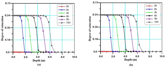Figure 1. (a) The curves of the RDITGCNFE solutions of infiltration moisture content at $t=2$ h, 4 h, ⋯, 10 h, respectively. (b) The curves of the TGCNFE solutions of infiltration moisture content at $t=2$ h, 4 h, ⋯, 10 h, respectively.

In order to explain that the RDITGCNFE format outbalances the TGCNFE format, we also find the TGCNFE solutions of infiltration moisture content at $t=2$ h, 4 h, ⋯, 10 h, as shown at Figure 1b. It is worth noting that, in the actual applications, it is not necessary to calculate the TGCNFE solutions, which can be replaced by the observations on the coarse grid division ${\Im }_H$ and fine grid division ${\Im }_h$ and to follow the above four steps directly to find the RDITGCNFE solutions.

It can be easily seen by comparing the curves in Figure 1a,b that the RDITGCNFE solutions are very closed to the TGCNFE solutions at $t=2$ h, 4 h, ⋯, 10 h.

By the above divisions ${\Im }_H$ and ${\Im }_h$, we can reckon that the TGCNFE format has $({10}^4+{10}^5)$ unknowns in each iteration, but the RDITGCNFE format has only $2\times 6$ unknowns in the same iteration. Hence, when the RDITGCNFE format is used to find the numerical solutions for the unsaturated soil water flow problem it can greatly reduce unknowns so as to greatly mitigate the calculated workload, save the CPU computing time, lessen the accumulation of computation errors, and enhance the computation efficiency.

In order to further reveal the advantages of the RDITGCNFE format, we recorded the errors and the CPU runtime of both TGCNFE and RDITGCNFE solutions at $t=2$ h, 4 h, ⋯, 10 h, calculated by Problems 6 and 7, respectively, as shown in Table 2.

Table 2. The CPU runtime and errors of the TGCNFE and RDITGCNFE solutions.

		TGCNFE Solutions		RDITGCNFE Solutions
$\mathit{t}$	$\mathit{k}$	Errors	CPU Runtime	Errors	CPU Runtime
2 h	720,000	$1.413612\times {10}^{-4}$	6348 s	$2.212436\times {10}^{-4}$	121 s
4 h	1,440,000	$2.827223\times {10}^{-4}$	12,697 s	$2.323865\times {10}^{-4}$	243 s
6 h	2,160,000	$4.240236\times {10}^{-4}$	19,145 s	$2.434971\times {10}^{-4}$	362 s
8 h	2,880,000	$5.653848\times {10}^{-4}$	25,394 s	$2.545943\times {10}^{-4}$	480 s
10 h	3,600,000	$7.028058\times {10}^{-4}$	31,745 s	$2.657882\times {10}^{-4}$	598 s

The errors for the TGCNFE solutions and the RDECNFE solutions in Table 2 are approximatively reckoned by $\parallel {\theta }_h^{k+1}-{\theta }_h^k{\parallel }_0$ and $\parallel {\theta }_d^{k+1}-{\theta }_d^k{\parallel }_0$, respectively, which are the accumulation of computation errors throughout the entire time domain.

The data of Table 2 have also signified that, as the time node moves forward, the CPU runtime to find the classical TGCNFE solutions (including 110,000 unknowns at each iteration) increased promptly, but the CPU runtime to find the RDITGCNFE solutions (only including 12 unknowns at the same iteration) increased very slowly. For example, when $t=10$ h, the CPU runtime for finding the classical TGCNFE solution is approximately 53 times that for finding the RDITGCNFE solution. In other words, the RDITGCNFE format can significantly save computation time. In addition, because the TGCNFE format contains too many unknowns, the errors of classical TGCNFE solutions gradually accumulate in the calculation process, while the RDITGCNFE format contains very few unknowns so that the errors of the RDITGCNFE solutions accumulate slowly. However, the numerical calculation errors are in agreement with the theory errors, both being $O({10}^{-4})$. It is further proven that the RDITGCNFE format is much better than the classical TGCNFE format and is valid for finding the solutions for the unsaturated soil water flow problem.

4.2. The Numerical Tests for the 10th Soil Parameters

As shown in Table 1, the 10th soil parameters imply that ${\theta }_s=0.60$, ${\psi }_s=-20$ cm, $K_s=1.6\times {10}^{-4}$ cm/s, $b=9.2$, and ${\theta }_r/{\theta }_s=0.487$. If still taking $Z=1000$ cm and the spatial step $h=0.01$ cm on the fine grid division ${\Im }_h$, we also divide $\overline{\Omega }=[0,1000]$ into 100,000 equal fine intervals. In order to meet $H^2=O(h)$, the coarse grid division ${\Im }_H$ is still taken as $H=0.1$ cm. The initial and boundary conditions of the unsaturated soil water flow problem are taken as follows:

$$\begin{array}{ccc}& & \left\{\begin{array}{cc}\theta (z,0)={\theta }_0(z)=0,\hfill & z\in [0,1000],\hfill \\ \theta (0,t)=0.60,\hfill & t\in (0,t_e],\hfill \\ \theta (1000,t)=\beta (t)=0,\hfill & t\in (0,t_e].\hfill \end{array}\right.\hfill \end{array}$$

Thus, if still taking the time step $\Delta t=0.01$ s, when $l=1$ and $\sqrt{{\lambda }_{Y(d_Y+1)}}=\sqrt{{\lambda }_{y(d_y+1)}}=O({10}^{-4})$, according to Theorems 2 and 4, the theory errors can also reach $O({10}^{-4})$.

The RDITGCNFE solutions of infiltration moisture content at $t=6$ h, 12 h, ⋯, 30 h for the unsaturated soil water flow problem may be found by the four steps in Section 4.1, as shown in the curves in Figure 2a.

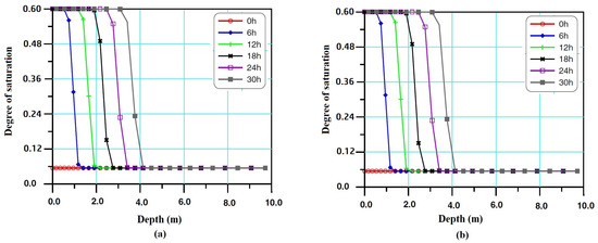
Figure 2. (a) The curves of the RDITGCNFE solutions of infiltration moisture content at $t=6$ h, 12 h, ⋯, 30 h, respectively. (b) The curves of the TGCNFE solutions of infiltration moisture content at $t=6$ h, 12 h, ⋯, 30 h, respectively.

In order to explain that the RDITGCNFE format outbalances the TGCNFE format, we also find the TGCNFE solutions of infiltration moisture content at $t=6$ h, 12 h, ⋯, 30 h, as shown in Figure 2b.

It can also be easily seen by comparing the curves in Figure 2a,b that the RDITGCNFE solutions are also very closed to the TGCNFE solutions at $t=6$ h, 12 h, ⋯, 30 h.

In order to further reveal the advantages of the RDITGCNFE format, we also recorded the errors and the CPU runtime for both the TGCNFE and RDITGCNFE solutions at $t=6$ h, 12 h, ⋯, 30 h, calculated by Problems 6 and 7, as shown in Table 3.

Table 3. The CPU runtime and errors of the TGCNFE and the RDITGCNFE solutions.

		TGCNFE Solutions		RDITGCNFE Solutions
$\mathit{t}$	$\mathit{k}$	Errors	CPU Runtime	Errors	CPU Runtime
6 h	2,160,000	$2.832523\times {10}^{-4}$	6348 s	$2.212436\times {10}^{-4}$	361 s
12 h	4,320,000	$4.665045\times {10}^{-4}$	19,046 s	$2.323865\times {10}^{-4}$	723 s
18 h	6,480,000	$6.797067\times {10}^{-4}$	38,089 s	$2.434971\times {10}^{-4}$	1085 s
24 h	8,640,000	$8.665094\times {10}^{-4}$	76,175 s	$2.545943\times {10}^{-4}$	1444 s
30 h	10,800,000	$9.863285\times {10}^{-4}$	95,220 s	$2.657882\times {10}^{-4}$	1806 s

The errors for the TGCNFE solutions and the RDECNFE solutions in Table 3 are also approximatively reckoned by $\parallel {\theta }_h^{k+1}-{\theta }_h^k{\parallel }_0$ and $\parallel {\theta }_d^{k+1}-{\theta }_d^k{\parallel }_0$.

The data of Table 3 have also further signified that when the time node moves forward, the CPU runtime for calculating the classical TGCNFE solutions (also including 110,000 unknowns at each iteration) increased promptly, but the CPU runtime for calculating the RDITGCNFE solutions (only including 12 unknowns at the same iteration) also increased very slowly. For example, when $t=30$ h, the CPU runtime for calculating the classical TGCNFE solution is also approximately 53 times that for calculating the RDITGCNFE solution, namely the RDITGCNFE format can significantly save computation time. Moreover, the TGCNFE format has too many unknowns so that the errors of classical TGCNFE solutions also gradually accumulate in the calculation process, while the RDITGCNFE format has very few unknowns so that the errors of the RDITGCNFE solutions also accumulate slowly. However, the numerical calculation errors are in agreement with the theory errors, both being $O({10}^{-4})$. It is proven once again that the RDITGCNFE format obviously outbalances the classical TGCNFE format and is beneficial for solving the unsaturated soil water flow problem.

5. Conclusions and Discussions

In this paper, we have designed a new TSDCN scheme and a new TGCNFE format as well as a new RDITGCNFE format for the unsaturated soil water flow problem. We have austerely demonstrated the existence and stability as well as the error estimates for the TSDCN solutions and the TGCNFE solutions as well as for the RDECNFE solutions, theoretically. We have also resorted to two sets of numerical tests to testify the rightness of the obtained theory results and exhibited the superiority of the RDITGCNFE format. It is worth noting that the TSDCN scheme and the TGCNFE format, as well as a new RDITGCNFE format for the unsaturated soil water flow problem, are first established in this paper. They are completely different from the existing formats. Without doubt, the RDITGCNFE format is also different from the existing POD-based FE reduced-dimension formats, with only first-order time precision and conditional convergence, such as the reduced-dimension format in [37]. Therefore, it is original and new.

Although we herein have developed the RDITGCNFE format for the unsaturated soil flow problem and simulated the moisture content of two types of soil parameters in Table 1, the method in this paper can simulate the moisture content of other types of soil parameters in Table 1 and can generalize to more complicated unsteady nonlinear PDEs, even actual engineering and industry problems, such as the axisymmetric rotating truncated cone made of functionally graded porous materials reinforced by graphene platelets under a thermal loading in [41]. Hence, the RDITGCNFE format has very capacious applied space.

However, because the RDITGCNFE method in this paper only includes the moisture content, it cannot directly calculate moisture flux for the unsaturated soil water flow problem. If the water flux is introduced as in the literature [37], and then the dimensionality reduction model including water content and water flux is established with the dimensionality reduction technique proposed in this paper, the dimensionality reduction solutions of moisture content and moisture flux can be calculated simultaneously. This will be a very interesting area of study.

References

- Xie, Z.; Zeng, Q.; Dai, Y.J.; Wang, B. Numerical simulation of an unsaturated flow equation. Sci. China Ser. D 1998, 41, 429–436. [Google Scholar] [CrossRef]
- Bear, J. Dynamics of Fluids in Porous Media; American Elsevier Publishing Company: New York, NY, USA, 1972. [Google Scholar]
- Lei, Z.D.; Yang, S.X.; Xie, S.C. Soil Hydrodynamics; Tsinghua University Press: Beijing, China, 1988. (In Chinese) [Google Scholar]
- Rahimi, A.; Rahardjo, H.; Leong, E. Effect of range of soil-water characteristic curve measurements on estimation of permeability function. Eng. Geol. 2015, 185, 96–104. [Google Scholar] [CrossRef]
- Li, Y.; Vanapalli, S.K. Models for predicting the soil-water characteristic curves for coarse and fine-grained soils. J. Hydrol. 2022, 612, 128248. [Google Scholar] [CrossRef]
- Yoon, S.; Chang, S.; Park, D. Investigation of soil-water characteristic curves for compacted bentonite considering dry density. Prog. Nucl. Energ. 2022, 151, 104318. [Google Scholar] [CrossRef]
- Dai, Y.; Zeng, Q. A land surface model (IAP94) for climate studies, Part I: Formulation and validation in off-line experiments. Adv. Atmos. Sci. 1997, 14, 433–460. [Google Scholar]
- Ye, D.; Zeng, Q.; Guo, Y. Contemporary Climatic Research; Climatic Press: Beijing, China, 1991. (In Chinese) [Google Scholar]
- Xie, Z.; Zeng, Q.; Dai, Y.; Wang, B. Application of finite element method to unsaturated soil flow problem. Clim. Environ. Res. 1998, 28, 73–81. [Google Scholar]
- Luo, Z.D.; Xie, Z.; Zhu, J.; Zeng, Q. Mixed finite element method and numerical simulation for the unsaturated soil water flow problem. Math. Numer. Sin. 2003, 25, 113–128. [Google Scholar]
- Ghannadi, P.; Kourehli, S.S.; Nguyen, A. The Differential Evolution Algorithm: An Analysis of More than Two Decades of Application in Structural Damage Detection (2001–2022). In Data Driven Methods for Civil Structural Health Monitoring and Resilience; CRC Press: Boca Raton, FL, USA, 2024; pp. 14–57. [Google Scholar]
- Xu, J. A novel two-grid method for semilinear elliptic equations. SIAM J. Sci. Comput. 1994, 15, 231–237. [Google Scholar] [CrossRef]
- Shi, D.; Liu, Q. An efficient nonconforming finite element two-grid method for Allen-Cahn equation. Appl. Numer. Math. 2019, 98, 374–380. [Google Scholar] [CrossRef]
- Shi, D.; Wang, R. Unconditional superconvergence analysis of a two-grid finite element method for nonlinear wave equations. Appl. Numer. Mat. 2020, 150, 38–50. [Google Scholar] [CrossRef]
- Luo, Z.; Chen, G. Proper Orthogonal Decomposition Methods for Partial Differential Equations; Academic Press of Elsevier: London, UK, 2019. [Google Scholar]
- Alekseev, A.K.; Bistrian, D.A.; Bondarev, A.E.; Navon, I.M. On linear and nonlinear aspects of dynamic mode decomposition. Int. J. Numer. Meth. Fl. 2016, 82, 348–371. [Google Scholar] [CrossRef]
- Du, J.; Navon, I.M.; Zhu, J.; Fang, F.; Alekseev, A.K. Reduced order modeling based on POD of a parabolized Navier-Stokes equations model II Trust region POD 4D VAR data assimilation. Comput. Math. Appl. 2013, 65, 380–394. [Google Scholar] [CrossRef]
- Li, H.; Song, Z. A reduced-order energy-stability-preserving finite difference iterative scheme based on POD for the Allen-Cahn equation. J. Math. Anal. Appl. 2020, 491, 124245. [Google Scholar] [CrossRef]
- Li, H.; Song, Z. A reduced-order finite element method based on proper orthogonal decomposition for the Allen-Cahn model. J. Math. Anal. Appl. 2021, 500, 125103. [Google Scholar] [CrossRef]
- Teng, F.; Luo, Z.D. A natural boundary element reduced-dimension model for uniform high-voltage transmission line problem in an unbounded outer domain. Comput. Appl. Math. 2024, 43, 106. [Google Scholar] [CrossRef]
- Zhu, S.; Dede, L.; Quarteroni, A. Isogeometric analysis and proper orthogonal decomposition for parabolic problems. Numer. Math. 2017, 135, 333–370. [Google Scholar] [CrossRef]
- Kunisch, K.; Volkwein, S. Galerkin proper orthogonal decomposition methods for a general equation in fluid dynamischs. SIAM J. Numer. Anal. 2002, 40, 492–515. [Google Scholar] [CrossRef]
- Li, K.; Huang, T.Z.; Li, L.; Lanteri, S.; Xu, L.; Li, B. A Reduced-Order Discontinuous Galerkin Method Based on POD for Electromagnetic Simulation. IEEE Trans. Antennas Propag. 2018, 66, 242–254. [Google Scholar] [CrossRef]
- Hinze, M.; Kunkel, M. Residual based sampling in POD model order reduction of drift-diffusion equations in parametrized electrical networks. J. Appl. Math. Mech. 2012, 92, 91–104. [Google Scholar] [CrossRef]
- Stefanescu, R.; Navon, I.M. POD/DEIM nonlinear model order reduction of an ADI implicit shallow water equations model. J. Comput. Phys. 2013, 237, 95–114. [Google Scholar] [CrossRef]
- Zokagoa, J.M.; Soulaǐmani, A. A POD-based reduced-order model for free surface shallow water flows over real bathymetries for Monte-Carlo-type applications. Comput. Methods Appl. Mech. Eng. 2012, 221–222, 1–23. [Google Scholar] [CrossRef]
- Baiges, J.; Codina, R.; Idelsohn, S. Explicit reduced-order models for the stabilized finite element approximation of the incompressible Navier-Stokes equations. Int. J. Numer. Meth. Fl. 2013, 72, 1219–1243. [Google Scholar] [CrossRef]
- Luo, Z.D. The reduced-order extrapolating method about the Crank–Nicolson finite element solution coefficient vectors for parabolic type equation. Mathematics 2020, 8, 1261. [Google Scholar] [CrossRef]
- Luo, Z.; Jiang, W. A reduced-order extrapolated technique about the unknown coefficient vectors of solutions in the finite element method for hyperbolic type equation. Appl. Numer. Math. 2020, 158, 123–133. [Google Scholar] [CrossRef]
- Zeng, Y.; Luo, Z. The reduced-dimension technique for the unknown solution coefficient vectors in the Crank–Nicolson finite element method for the Sobolev equation. J. Math. Anal. Appl. 2022, 513, 126207. [Google Scholar] [CrossRef]
- Luo, Z. A finite element reduced-dimension method for viscoelastic wave equation. Mathematics 2022, 10, 3066. [Google Scholar] [CrossRef]
- Luo, Z. The dimensionality reduction of Crank–Nicolson mixed finite element solution coefficient vectors for the unsteady Stokes equation. Mathematics 2022, 10, 2273. [Google Scholar] [CrossRef]
- Yang, X.; Luo, Z. An unchanged aasis function and preserving accuracy Crank-Nicolson finite element reduced-dimension method for symmetric tempered fractional diffusion equation. Mathematics 2022, 10, 3630. [Google Scholar] [CrossRef]
- Lumley, J.L. Coherent Structures in Turbulence, Transition and Turbulence; Meyer, R.E., Ed.; Academic Press: New York, NY, USA, 1981; pp. 215–242. [Google Scholar]
- Fukunaga, K. Introduction to Statistical Recognition; Academic Press: New York, NY, USA, 1990. [Google Scholar]
- Jolliffe, I. Principal Component Analysis; Springer: Berlin/Heidelberg, Germany, 2002. [Google Scholar]
- Luo, Z.D.; Li, Y.J. A preserving precision mixed finite element dimensionality reduction method for unsaturated flow problem. Mathematics 2022, 10, 4391. [Google Scholar] [CrossRef]
- Luo, Z. The Foundations and Applications of Mixed Finite Element Methods; Chinese Science Press: Beijing, China, 2006. (In Chinese) [Google Scholar]
- Zhang, G.; Lin, Y. Notes on Functional Analysis; Peking University Press: Beijing, China, 2011. (In Chinese) [Google Scholar]
- Zhang, W. Finite Difference Methods for Patial Differential Equations in Science Computation; Higher Education Press: Beijing, China, 2006. (In Chinese) [Google Scholar]
- Babaei, M.; Kiarasi, F.; Asemi, K.; Dimitri, R.; Tornabene, F. Transient thermal stresses in FG porous rotating truncated cones reinforced by graphene platelets. Appl. Sci. 2022, 12, 3932. [Google Scholar] [CrossRef]
Disclaimer/Publisher’s Note: The statements, opinions and data contained in all publications are solely those of the individual author(s) and contributor(s) and not of MDPI and/or the editor(s). MDPI and/or the editor(s) disclaim responsibility for any injury to people or property resulting from any ideas, methods, instructions or products referred to in the content. |
© 2024 by the authors. Licensee MDPI, Basel, Switzerland. This article is an open access article distributed under the terms and conditions of the Creative Commons Attribution (CC BY) license (https://creativecommons.org/licenses/by/4.0/).