An Augmented Social Network Search Algorithm for Optimal Reactive Power Dispatch Problem

Abstract

Optimal Reactive Power Dispatch (ORPD) is one of the main challenges in power system operations. ORPD is a non-linear optimization task that aims to reduce the active power losses in the transmission grid, minimize voltage variations, and improve the system voltage stability. This paper proposes an intelligent augmented social network search (ASNS) algorithm for meeting the previous aims compared with the social network search (SNS) algorithm. The social network users’ dialogue, imitation, creativity, and disputation moods drive the core of the SNS algorithm. The proposed ASNS enhances SNS performance by boosting the search capability surrounding the best possible solution, with the goal of improving its globally searched possibilities while attempting to avoid getting locked in a locally optimal one. The performance of ASNS is evaluated compared with SNS on three IEEE standard grids, IEEE 30-, 57-, and 118-bus test systems, for enhanced results. Diverse comparisons and statistical analyses are applied to validate the performance. Results indicated that ASNS supports the diversity of populations in addition to achieving superiority in reducing power losses up to 22% and improving voltage profiles up to 90.3% for the tested power grids.

1. Introduction

1.1. Motivation

With the recent massive increase in the cost of petroleum fuel and its direct and indirect impact on people’s daily lives, focus has shifted to optimizing active and reactive power flow in order to improve the economics and security of power system operations. Furthermore, increasing power consumption is critical for assisting the electrical power industry in planning and ensuring the appropriate operation of electrical power infrastructure [1,2]. Optimal Power Flow (OPF) is a non-convex, non-continuous, non-linear, large-scale, and constrained optimization problem through which control variables are optimized while satisfying both equality and inequality constraints.

The process of reaching parameter values that minimize the overall function is called optimization. Most search algorithms suffer from local minimum where the algorithm manages to find the minimal value within the nearby points but perhaps fails to reach the minimal value in all other possible places in the problem state space. The key point is to find global optima. Global optimization is a major issue that faces search algorithms. The key motivation of this research is to reach a global optima in the ORPD problem work space [3].

ORPD is one of the challenges of OPF and one of the most important responsibilities in the power system network operation [3,4]. The primary goal of the ORPD is to reduce real power losses and voltage variations while improving system voltage stability, considering several equality and inequality constraints, including voltages of generators, power flows through the lines, voltages of load buses, reactive power production, and transformer taps. Furthermore, ORPD aims to determine the best-operating settings of the control variables, such as transformer tap, generator voltage, and the number of compensation devices to be switched [5].

1.2. Literature Review

In recent years, a range of novel and meta-heuristic optimization techniques have been effectively presented for solving engineering problems. They are becoming increasingly prominent in several academic fields for tackling difficult optimization problems. These stochastic techniques are applied in several aspects of power system optimization. An improved chaotic harmony search optimizer has been introduced, integrating the chaotic patterns for generating random numbers with uniform distribution to solve the dispatch problem while combining environmental and economic objectives [6]. In [7], a biogeography-based optimizer (BBO) has been used for OPF issues with valve point non-linearities, but it has only been evaluated for small IEEE 9-bus and 30-bus systems. In [8], a modified version of the Slime-Mould algorithm (SMA) has been applied to solve the economic-emission dispatch problem, with updated equations from the sine–cosine technique included to increase the SMA’s performance. In addition, a moth flame algorithm has been utilized for the unit commitment problem in order to find the optimal scheduling of the generation units [9]. Furthermore, an artificial gorilla algorithm has been developed for solving the multi-dimensional optimal power flow problem [10], while a genetic algorithm combining a time series has been presented to search for the optimal allocation of reactive power compensation devices considering the impacts of distributed generators [11].

Over the past few years, many optimizers have been introduced to tackle the ORPD issues. Conventional optimization approaches such as linear programming [12], the Newton method [13], quadratic programming [14], and the interior-point method [15] were the most widely employed optimizers in the early years. In [16], a fuzzy-based procedure (FLP) approach was used to maximize the impact of preventive control activities related to reactive power to overcome any emergency circumstance that arose. FLP was used in this work to reduce violation limitations and provide an appropriate reactive power reserve for multi-operating scenarios. However, these approaches frequently have drawbacks, such as converging to the nearest optimum, incapability of dealing with non-linear and non-convex limitations, discontinuity forms of objective functions, and situations with many local minimum locations. As a result, new strategies for overcoming these limitations have to be developed.

Evolutionary computing optimizers have been used for solving the ORPD as QEA [17], PSO [18], hybrid PSO [19], BFA [20], adaptive real-coded GA [21], CLPSO [22], harmony search algorithm [23], GSA [24], DE algorithm [25], hybrid PSO and ICA [26], and exchange market algorithm [27].

Recently, a novel improved ALO algorithm [28,29], GB-WCA [30], multi-objective ALO algorithm [31], hybrid swarm intelligence [32], enhanced teaching learning-based optimization algorithm [33], ILAO [34], tunicate swarm algorithm [35], and AEO [36] have been employed to solve the OPRD with consideration of different constraints. In [37], an improved variant of the evaporation rate water cycle algorithm (ERWCA) has been presented to regulate the directional overcurrent relays in power systems. In this study, an oppositional learning strategy with Levy-flight was incorporated into ERWCA to prevent landing on the local optimum and increase the convergence rate, and it was validated on the CEC’2017 test suite and compared to other algorithms. In [38], a beetle antenna search algorithm was implemented to address the optimal active power dispatch in addition to enhancing the electrical performance of power networks by reducing fuel expenditure, air pollution, and power losses.

In The hybrid multi-swarm PSO algorithm was demonstrated in [25] to overcome the problem of OPRD while increasing the voltage profile and reducing real power loss. In [39], the EFA has been utilized to solve the ORPD and optimally active problems. In [40], the MODE has been characterized as solving the OPRD by reducing the power loss, the voltage deviation, and increasing the voltage stability. In [41], the convex quadratic optimization program has been elaborated to sustain the voltage bus even in the unbalanced distribution system. In [42], QODE has been successfully applied to solve the ORPD problem by reducing the power loss, improving the voltage profile, and increasing the voltage stability.

While in [43], FA has been combined with the APT-FPSO and applied to the ORPD problem with IEEE 30-bus, IEEE 57-bus, and IEEE 118-bus, considering the voltage stability index and voltage magnitude deviations. In [44], the ABC algorithm has been applied on ORPD IEEE 30- and 57-bus grids with consideration of voltage stability enhancement, real power loss minimization, and voltage deviation minimization. In [45], SHADE has been applied to ORPD IEEE 30-bus and 57-bus with steady-state voltage deviation and real power loss. To address the reactive power flow issue in power systems, accelerated bio-inspired optimization (ABO) was used [46]. Despite the fact that the results were significant, the obtained operating points in this study required feasibility validations.

In [47], a SCA was being used to handle the ORPD issue more efficiently than other meta-heuristic techniques. However, because this was a single objective minimization work, only power losses were considered. In [48], a WOA has been utilized to solve the ORPD task with applications on the IEEE 14-bus, IEEE 30-bus, and practical Algerian electrical network. In this study, the performance of WOA showed efficient performance compared to PSO and PSO-TVAC. However, the reported comparisons were only performed as a single objective optimization for network losses. In [49], a SBDE algorithm has been presented to handle the ORPD issue and achieve the maximum reduction of grid losses. However, the performance assessment of the presented SBDE algorithm compared with the GA was only applied to small grids of IEEE 14- and IEEE 30-bus grids.

In 2022, different studies have been proposed to solve ORPD issues, as in [50], an IMPA is introduced. IMPA improved the marine predator algorithm exploration and exploitation techniques by updating the predator position to be near the best predator using spiral movement. The IMPA was only tested using the IEEE 30-bus system and showed superiority over the original MPA. In [51], the CTFWO algorithm was introduced. The CTFWO algorithm enhances the exploration rate of the conventional TFWO using chaotic maps. The CTFWO was tested on two bus systems, the IEEE 30-bus and IEEE 57-bus. In [52], the authors introduced the CAC-DE hybrid approach, through which the best compromise solution is found using Fuzzy Logic. CAC-DE has effectively reduced the power loss, but it has not performed the same for the Voltage Stability Index. Furthermore, the authors proposed new algorithms in radial distribution networks for reducing energy loss and capacitor investment in order to reduce costs [53]. They proposed a hybridization of evolutionary algorithms with a sensitivity-based decision-making technique for the optimal planning of shunt capacitors [54] and a novel combined evolutionary algorithm for the optimal planning of distributed generators [55]. Finally, ref. [56] finds optimal solutions for the placement of reactive and active power generation components in distribution networks using a high-performance meta-heuristic algorithm.

1.3. Research Gap

The SNS algorithm was driven by social networking participants in various moods such as imitation, discussion, disputation, and creativity in attitudes used to express people’s new ideas on current events [57]. To begin, an imitation mood is created in which people must evaluate the viewpoints of other individuals in order to copy other users in expressing their particular opinions. Secondly, the dialogue mood is simulated, in which people may link and share the perspectives of others. Thirdly, the disputation mood is simulated, in which people can debate their opinions with a group of other users. Fourthly, the creativity mood is simulated, in which people analyze a topic that is generally related to their fresh convictions. According to [58], the SNS algorithm was used for OPF in its traditional configuration, but its related reliability required additional supports and adaptations in the fields of power simulations and optimizations, mathematical benchmarking frameworks, and complex engineering challenges. As a result, in this article, an ASNS algorithm for multi-dimensional ORPD in power grids is presented. Two enhancements are incorporated to improve the performance of the SNS algorithm. In the beginning, an effective exploitation strategy is intended to increase the seeking of the best view by all users. Second, because exploiting support is necessary towards the end of iterations, an adjustable variable is provided for this procedure. As this value grows, so does the level of support for the exploiting feature provided by the offered effective strategy [59].

1.4. Problem Statement

ORPD is one of the most important responsibilities in power system network operations. It targets determining the best-operating settings of the control variables, such as transformer tap, generator voltage, and the number of compensation devices to be switched. The primary goal of the ORPD is to reduce real power losses and voltage variations while improving system voltage stability. Several equality and inequality constraints must be handled, including voltages of generators, power flows through the lines, voltages of load buses, reactive power production, and transformer taps.

1.5. Major Contributions of this Study and Paper Organization

The following are the major contributions described in this work:

• A novel ASNS algorithm with an effective exploitation strategy is introduced.
• A novel ASNS algorithm-inspired scheme for handling the ORPD problem is offered and scrutinized on three typical IEEE test grids of different sizes.
• A test is executed to authenticate the statistical efficacy of the suggested ASNS-inspired scheme.
• The suggested ASNS algorithm presents a robust and straightforward solution for the ORPD problem under two-goal functions of minimizing grid losses and voltage deviations.
• The simulation results disclose the dominance of the suggested ASNS algorithm over many solvers that were recently reported in the literature.

The following portions of this work are organized as follows: Section 2 presents the design framework for the ORPD optimization problem. Section 3 also establishes the basic SNS and the suggested ASNS, whereas Section 4 defines the discussions and simulation findings. Finally, Section 5 concludes this paper.

2. ORPD Formulation

In the ORPD issue, the decision variables are the generator voltages that are denoted by (VG₁, VG₂, …, VG_NG), the transformer tap settings that are denoted by (Ta₁, Ta₂, …, Ta_NT), and the reactive power (VAr) supplied by switched capacitors and reactors, which are denoted by (Qr₁, Qr₂, …, Qr_Nr), respectively. The values NG, Nr, and NT indicate the number of generators, the number of VAr sources, and the number of on-load tap transformers. The dependent variables include load bus voltage magnitudes, VAr outputs of the generators, and transmission line loadings, which are demonstrated by (VL₁, …, VL_NPQ), (QG₁, QG₂, …, QG_NG), and (SF₁, …, SF_NL), respectively. The values NPQ and NL indicate the number of load buses and the number of transmission lines. As a result, the ORPD problem may be mathematically stated as shown in the following equation:

$$\begin{gathered} {\mathit{Min} F}_n={\{f}_1{(X}_u{,X}_v{),f}_2{(X}_u{,X}_v)\} \\ \mathrm{Subjected} \mathrm{to}: {M(X}_u{,X}_v)=0 \mathrm{and} {N(X}_u{,X}_v)\le 0 \end{gathered}$$

(1)

2.1. Problem Objectives

The primary goal of the ORPD issue is to reduce two technical objectives: real power losses in the transmission grid and voltage variations across the buses. Therefore, both technical objectives are investigated as follows:

2.1.1. Total Grid Losses

The minimization of TGLs in MW can be computed as [60]:

$$TGLs={\displaystyle \sum _{i=1}^{Nb}{\displaystyle \sum _{j=1}^{Nb}{G}_{ij}{(V}_i{}^2{+V}_j{}^2}-{2(V}_i{V}_j{cos \theta }_{ij})}$$

(2)

2.1.2. Voltage Profile Improvement

The voltage profile gets improved by reducing the total voltage deviation (TVD) for the buses by 1 p.u. as follows:

$$VD={\displaystyle \sum _{i=1}^{N_b}\left|V_i-V_{ref}\right|}$$

(3)

2.1.3. Voltage Stability Improvement

This objective function is introduced in order to improve voltage stability by decreasing the maximum voltage stability index (L-index), which is used in [61]. The L-index for each bus j (L_j) is established as follows:

$$L_j=\left|1-{\displaystyle \sum _{i=1}^{N_g}{F}_{ji}\frac{V_i}{V_j}\angle ({\theta }_{ij}+{\delta }_i-{\delta }_j)}\right|$$

(4)

$$F_{ji}={\left[Y_{LL}\right]}^{-1}\left[Y_{LG}\right]$$

(5)

To increase the system’s VSI, the maximum L-index should be reduced as follows:

$$VSI=Max (L_j)j=1,2,........N_b$$

(6)

2.2. Problem Constraints

2.2.1. The Inequality Constraints

The power system has to satisfy different inequality constraints corresponding to the operational variables. For the decision variables, Equations (7)–(9) describe the inequality constraints of the generator voltages, the transformer tap settings, and the reactive power injected into switched capacitors and reactors, respectively [62].

$${VG}_{{}_k}^{min}\le {VG}_{{}_k}\le {VG}_{{}_k}^{max}, k=1:NG$$

(7)

$${Ta}_l^{min}\le {Ta}_l\le {Ta}_l^{max}, l=1:NT$$

(8)

$${Qr}_s^{max}\le {Qr}_s\le {Qr}_s^{max}, s=1:Nr$$

(9)

For the dependent variables, Equations (10)–(12) describe the inequality constraints of the load bus voltage magnitudes, the reactive power outputs of the generators, and transmission line loadings, respectively:

$${VL}_m^{min}\le {VL}_m\le {VL}_m^{max}, m=1:NPQ$$

(10)

$$\left|{SF}_L\right|\le {SF}_L^{max}, L=1:NL$$

(11)

$${QG}_{{}_k}^{min}\le {QG}_{{}_k}\le {QG}_{{}_k}^{max}, k=1:NG$$

(12)

2.2.2. The Equality Constraints

These constraints are represented by the load flow balance equations, as denoted in Equations (13) and (14):

$${Pg}_i-{PL}_i-V_i{\displaystyle \sum _{j=1}^{Nb}{V}_j}{(G}_{ij}{cos \theta }_{ij}+B_{ij}{sin \theta }_{ij})=0, i=1, \dots , \mathit{Nb}$$

(13)

$${\mathit{Qg}}_i-{\mathit{QL}}_i+{\mathit{Qr}}_i-V_i{\displaystyle \sum _{j=1}^{\mathit{Nb}}{V}_j}{(G}_{\mathit{ij}}{\mathit{sin}\theta }_{\mathit{ij}}-B_{\mathit{ij}}{\mathit{cos}\theta }_{\mathit{ij}})=0, i=1,2, \dots , \mathit{Nb}$$

(14)

where Pg_i is the output power of each generator (i); PL_i and QL_i are the active and reactive power demands of each load (i); B_ij is the mutual susceptance between bus i and j, respectively; G_ij is the conductance of every line connecting buses i and j; θ, V, and N_b are the phase angle, voltage, and number of buses, respectively; and Qg_i is the VAr output of each generator (i).

3. Proposed ASNS for Solving the ORPD Problem

3.1. Basic SNS Algorithm

The SNS framework is derived from participants on social networking sites, where people try to be attractive and express a variety of moods [57]. Such attitudes are techniques for sharing people’s fresh perspectives on a new occurrence. Firstly, the imitation mood is simulated, in which people must consider the perspectives of various individuals to emulate other users in expressing their personal thoughts. Secondly, the dialogue mood is simulated, in which people may link and share the perspectives of others. Thirdly, the disputation mood is simulated, in which people can debate their opinions with a group of other users. Fourthly, the creativity mood is simulated, in which people analyze a topic that is generally related to their fresh convictions. The four inspired moods of the SNS are mathematically described as:

3.1.1. Imitation

If there is a new event with an interesting notion, members can imitate renowned people by attempting to publish a thread that discusses this topic. This state of mind could be expressed as follows:

$$U_{i,new}=U_j+r_1\times r_2\times (U_i-U_j)$$

(15)

3.1.2. Dialogue

People may learn more about an event by exchanging thoughts with one another from various points of view and then generating a fresh perspective on the event. This state of mind can be expressed numerically as:

$$U_{i,new}=U_k+r_1\times [sign(f_i-f_j)(U_i-U_j)]$$

(16)

The term [sign(f_i − f_j)(U_i − U_j)] illustrates the diversity in the viewpoints of the users.

3.1.3. Disputation

People in this mood can communicate and advocate their viewpoints with remarks or discussions; however, they could be persuaded by other established commentators to exchange ideas about a specific issue. This state of mind can be expressed as:

$$U_{i,new}=U_i+r_1\times \left[U_{mean}-((1+round(r_1))\times U_i)\right]$$

(17)

where the mean vector within a group or commenters’ views of friends is defined in Equation (18):

$$U_{mean}=\frac{1}{N_{group}}{\displaystyle \sum _{u=1}^{N_{group}}{U}_u}$$

(18)

3.1.4. Creativity

Users can express themselves creatively and innovatively regarding a given topic. As a result, a fresh concept will be generated, and this mood can be expressed as:

$$U_{i,new}^d=t_2{U}_j^d+(1-r_2)(r_1\times (U{B}^d-L{B}^d)+L{B}^d)$$

(19)

3.1.5. Rules Related to the Network

Each social network defines a set of roles for its users, and these roles are regarded by all users from shared perspectives. The following factors are used to limit the users’ perspectives:

$$U_{k,new}=\min (U_{k,new},U{B}_k)\&U_{k,new}=\max (U_{k,new},L{B}_k),k=1:D$$

(20)

3.1.6. Rules for Publishing

The SNS method is produced by various moods, in which every user’s viewpoint is modified and fresh views are adopted based on their merit. To demonstrate, if the new idea is superior to the existing one, it will be approved. As a result, the value of a new idea can be quantitively estimated by its fitness function as follows:

$$U_i=\{\begin{array}{ll}{U}_i& f(U_{i,new})>f(U_i)\\ U_{i,new}& f(U_{i,new})<f(U_i)\end{array}$$

(21)

To design SNS, the starting viewpoint for every user may be created as:

$$U_0=(rand(0,1)\times (UB-LB))+LB$$

(22)

3.2. ASNS with an Effective Exploitation Strategy

To increase the performance of the algorithm, an ASNS algorithm with EES is used. The performance of the SNS algorithm is improved with two adjustments. In the beginning, an EES is intended to improve the search capability for of all users. As a result, the basic SNS’s upgrading process has been adjusted, and the viewpoints of many users have been altered as follows:

$$U_{i,new}^d=U_{best}^d+t\times r$$

(23)

$$r=U_i-U_j$$

(24)

$$t=rand(0,1)$$

(25)

Second, because exploitation support is required at the end of iterations, an adjustable parameter (α) is created using Equation (26) [63,64]:

$$\alpha =\frac{t}{2\ast T^{\mathit{max}}}$$

(26)

Using this formula, this parameter is grown directly proportional to the number of iterations until it reaches 0.5 of its upper level. The offered EES gives more support for the exploitative feature as this value increases. The suggested EES in Equation (26) is not engaged until more than half of the iterations have been completed, as indicated in [64]. As a consequence of this stance, the ASNS’s superior diversifying skills in uncovering newer prospective sectors are retained. Moreover, since the variable (α) grows directly proportional to the number of repetitions, the proposed EES is integrated with increasing likelihood. Consequently, the greater the number of repetitions, the further the search is reduced to the region encircling the user’s greatest viewpoint. This phase fosters exploitation while simultaneously enabling the discovery of a diverse variety of new viable locations.

According to this method, considerable assistance aims at boosting the search capability of the basic SNS algorithm to surround the best perspective solution, to improve its globally searching possibilities, and to avoid getting locked in a locally optimal solution.

3.3. Proposed ASNS with EES for Solving the ORPD Problem

When dealing with the mentioned ORPD problems, the equality and inequality restrictions are considered. The NRA is used to meet the equality criteria that defines power flow balancing equations. It represents the steady-state operation of electricity networks and satisfies the balancing restrictions.

As a result, the NRA, which is employed by MATPOWER, constitutes a critical foundation for showing three-phase power grids [65]. Furthermore, the decision/dependent variable constraints must be preserved. The operational limitations of independent variables in Equations (7)–(9) can be rewritten as follows:

$$V{G}_{{}_i}=\{\begin{array}{cc}V{G}_i^{\min }& if V{G}_{{}_i}\le V{G}_{{}_i}^{\min }\\ V{G}_{{}_i}^{\max }& if V{G}_{{}_i}\ge V{G}_i^{\max }\end{array}, i=1:NG$$

(27)

$$T{a}_l=\{\begin{array}{cc}T{a}_l^{\min }& if T{a}_l\le T{a}_l^{\min }\\ T{a}_l^{\max }& if T{a}_l\ge T{a}_l^{\max }\end{array}, l=1:NT$$

(28)

$$Q{r}_s=\{\begin{array}{cc}Q{r}_s^{\min }& if Q{r}_s\le Q{r}_s^{\min }\\ Q{r}_s^{\max }& if Q{r}_s\ge Q{r}_s^{\max }\end{array}, s=1:Nr$$

(29)

As demonstrated, the variables keep reaching their limits; however, if one of them exceeds the limit, it is reproduced at random within the necessary bounds. Furthermore, the fitness function broadens and penalizes the restrictions of the second classification. As a result, if the user vectors surpass any of the relevant limitations, they will be eliminated in the following round. As stated in Equation (30), those notions can be utilized to create the considered fitness.

$$F=f_j+Pe{n}_1{\displaystyle \sum _{m=1}^{NPQ}\Delta V{L}_m^2}+Pe{n}_2{\displaystyle \sum _{L=1}^{NPQ}\Delta S{F}_L^2}+Pe{n}_3{\displaystyle \sum _{k=1}^{NPQ}\Delta Q{G}_k^2}$$

(30)

where f_j indicates each fitness function; Pen₁ is the penalty coefficient for any violation in load voltage; Pen₂ is the penalty coefficient for any violation in reactive power output from generators; and Pen₃ is the penalty coefficient for any violation in line power flow. Where ΔVL_m, ΔSF_L, and ΔQG_k are presented as:

$$\Delta V{L}_m=\{\begin{array}{cc}V{L}_m^{\min }-V{L}_m& if V{L}_m<V{L}_m^{\min }\\ V{L}_m^{\max }-V{L}_m& if V{L}_m>V{L}_m^{\max }\end{array}$$

(31)

$$\Delta S{F}_L=S{F}_L^{\max }-S{F}_L if S{F}_L>S{F}_L^{\max }$$

(32)

$$\Delta Q{G}_k=\{\begin{array}{cc}Q{G}_k^{\min }-Q{G}_k& if Q{G}_k<Q{G}_k^{\min }\\ Q{G}_k^{\max }-Q{G}_k& if Q{G}_k>Q{G}_k^{\max }\end{array}$$

(33)

Figure 1 displays the stages of the designed ASNS for ORPD.

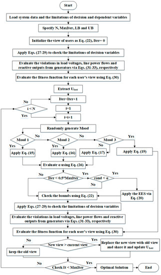
Figure 1. Proposed ASNS for solving the ORPD problem.

4. Simulation Results

Three distinct standard IEEE grids were utilized as case studies for comparative purposes to investigate the capacity to handle the ORPD challenge as well as the resilience of the suggested ASNS in finding high-quality solutions. The SNS and ASNS algorithms were implemented in the MATLAB software language. The data for three power grids are provided in Table 1, and the entire dataset is derived from [29], while all the limits on control variables used here for all test systems are summarized in Appendix A. The three power grids represent real case studies, where the IEEE 30-bus grid test case represents a simple approximation of the American Electric Power system, while the IEEE 57-bus and IEEE 118-bus grids represent simple approximations of the American Electric Power system in the U.S. Midwest [66].

Table 1. Information from the studied systems.

Case Study	Number of Branches	Number of Loads	Number of Generators	Number of Control Variables	Number of Transformers	Number of Compensators
IEEE 30-bus grid	41	24	6	19	4	9
IEEE 57-bus grid	80	50	7	25	15	3
IEEE 118-bus grid	186	64	54	75	9	12

The SNS and the suggested ASNS algorithms were implemented by adjusting the size of the population and the maximum number of iterations to 50 and 300 for the first grid, 100 and 300 for the second grid, and 100 and 600 for the third grid.

The relation of proposed method parameters to system parameters can be clearly described with Equation (34):

$$Population=\left[\begin{array}{lll}V{G}_{1,i}(i=1:NG)& T{a}_{1,l}(l=1:NT)& Q{r}_{1,s}(s=1:Nr)\\ V{G}_{2,i}(i=1:NG)& T{a}_{2,l}(l=1:NT)& Q{r}_{2,s}(s=1:Nr)\\ .& & \\ .& & \\ V{G}_{N,i}(i=1:NG)& T{a}_{N,l}(l=1:NT)& Q{r}_{N,s}(s=1:Nr)\end{array}\right]$$

(34)

The findings of each approach were acquired for each study case by executing 30 tests. The following two cases are being investigated:

• Case 1: Minimization of the TGLs described in Equation (2).
• Case 2: Minimization of the TVD described in Equation (3).
• Case 3: Minimization of the VSI described in Equation (6).

4.1. Results of the First Grid

As illustrated in Figure 2, this grid comprises of 30-bus and 41-branch generators, 4 on-load tap changing transformers, and 9 shunted compensators. The entire dataset for lines, buses, and the limits of reactive power generation is utilized [67,68]. The limits for the generator voltage and tap settings are 1.1000 and 0.9000 p.u., respectively. The limits of voltage for the load buses are considered to be 1.0500 and 0.9500 p.u., respectively. The SNS and proposed ASNS algorithms are implemented in the first case, and the best control settings are presented in Table 2. The basic SNS algorithm reduces TGLs from 5.7960 MW to 4.5208 MW when compared to the initial case; however, the proposed ASNS algorithm achieves the lowest power losses of 4.5206 MW when compared to 5.7960 MW in the initial instance. This is a 22% reduction. The resulting solutions are contrasted with previously reported findings for minimizing the losses and utilizing the same circumstances, as summarized in Table 2, which shows that the proposed ASNS algorithm outperforms numerous strategies in minimizing the TGLs. ILAO [34], SCA [47], WOA [48], HFA [69], QOTLBO [70], CLPSO [22], ABC [28], ALO [28], MPA [50], MFA [71], and AEO [36] achieve TGLs of 4.5217, 4.7086, 4.5943, 4.529, 4.5594, 4.5615, 4.6110, 4.5900, 4.5335, 4.5340, and 4.5262, respectively.

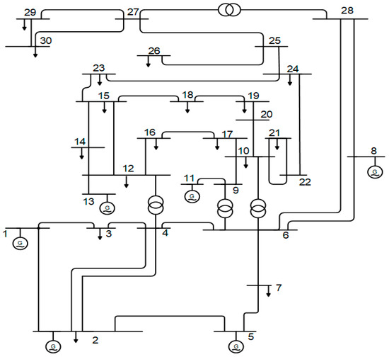
Figure 2. IEEE 30-bus grid [72].

Table 2. Optimal results for Case 1 of the IEEE 30-bus grid.

Variables	Initial Case	SNS	Proposed ASNS	ILAO * [34]	SCA * [47]	WOA * [48]	HFA * [69]
VG 1	1.0500	1.1000	1.0999	1.1000	1.1000	1.1000	1.1000
VG 2	1.0400	1.0946	1.0941	1.0944	1.1000	1.0963	1.0543
VG 5	1.0100	1.0751	1.0741	1.0944	1.0869	1.0789	1.0751
VG 8	1.0100	1.0768	1.0759	1.0767	1.0870	1.0774	1.0869
VG 11	1.0500	1.0544	1.0907	1.1000	1.1000	1.0955	1.1000
VG 13	1.0500	1.0905	1.0824	1.1000	1.0800	1.0929	1.1000
Ta 6–9	1.0780	1.0746	0.9871	1.0300	1.0500	0.9936	0.9801
Ta 6–10	1.0690	0.9080	1.0185	0.900	1.0500	0.9867	0.9500
Ta 4–12	1.0320	1.0000	0.9992	0.9800	1.0500	1.0214	0.9702
Ta 28–27	1.0680	0.9686	0.9669	0.9600	1.0500	0.9867	0.9700
Qr 10	0.0000	16.6738	11.8166	4.9900	4.6310	3.1695	4.7003
Qr 12	0.0000	19.4818	24.57618	5.0000	3.0890	2.0477	4.7061
Qr 15	0.0000	3.9071	3.7694	5.0000	5.0000	4.2956	4.7007
Qr 17	0.0000	5.5106	5.4730	5.0000	4.6970	2.6782	2.3059
Qr 20	0.0000	4.0268	3.5115	3.8000	2.1290	4.8116	4.8035
Qr 21	0.0000	9.7636	10.0785	5.0000	3.1910	4.8163	4.9026
Qr 23	0.0000	0.9029	1.3975	3.3500	5.0000	3.5739	4.8040
Qr 24	0.0000	6.8624	6.6386	5.0000	4.3880	4.1953	4.8053
Qr 29	0.0000	2.2385	2.1505	1.4400	3.5750	2.0009	3.3984
TGLs	5.7960	4.5208	4.5206	4.5217	4.7086	4.5943	4.5290
Variables	QOTLBO * [70]	CLPSO * [22]	ABC * [28]	MFA * [71]	AEO * [36]	ALO * [28]	MPA * [50]
VG 1	1.1000	1.1000	1.1000	1.1000	1.1000	1.1000	1.1000
VG 2	1.0942	1.1000	1.0971	1.0943	1.0944	1.0953	1.0949
VG 5	1.0745	1.0795	1.0866	1.0747	1.0751	1.0767	1.0761
VG 8	1.0765	1.1000	1.0800	1.0766	1.077	1.0788	1.078
VG 11	1.1000	1.1000	1.0850	1.1000	1.1000	1.1000	1.0873
VG 13	1.0999	1.1000	1.1000	1.1000	1.1000	1.1000	1.1000
Ta 6–9	1.0664	0.9154	1.0700	1.0433	1.0392	1.0100	0.9807
Ta 6–10	0.9000	0.9000	0.9500	0.9000	0.9000	0.9900	1.0222
Ta 4–12	0.9949	0.9000	1.0200	0.9791	0.9729	1.0200	0.9765
Ta 28–27	0.9714	0.9397	1.1000	0.9647	0.9632	1.0000	0.9707
Qr 10	5.0000	4.9265	5.0000	5.0000	4.9948	4.0000	1.7900
Qr 12	5.0000	5.0000	0.0000	5.0000	4.9963	2.0000	4.8300
Qr 15	5.0000	5.0000	2.0000	4.8055	4.8409	4.0000	3.9700
Qr 17	5.0000	5.0000	5.0000	5.0000	4.9985	3.0000	4.9900
Qr 20	4.4500	5.0000	4.0000	4.0623	4.2895	2.0000	4.2200
Qr 21	5.0000	5.0000	5.0000	5.0000	5.0000	4.0000	4.6100
Qr 23	2.8300	5.0000	4.0000	2.5193	2.6464	3.0000	4.6900
Qr 24	5.0000	5.0000	5.0000	5.0000	4.9998	5.0000	4.1200
Qr 29	2.5600	5.0000	4.0000	2.1925	2.2293	5.0000	3.2900
TGLs	4.5594	4.5615	4.611	4.5340	4.5262	4.59	4.5335

* The techniques in the comparisons are not coded by the authors but are employed by their creators.

Furthermore, the convergent properties of the proposed ASNS and SNS for Case 1 of the IEEE 30-bus grid are depicted in Figure 3. As shown, the curve describes the minimization of the total power losses throughout the iterations, while the small shape provides a zoning on the range [4.5–4.85] MW. The variation of the losses starts at a high value of 6.4500 MW at the fifth iteration and continues decreasing, reaching 4.5892, 4.5313, and 4.5206 MW at iterations 100, 200, and 300, respectively.

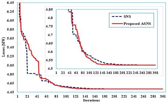
Figure 3. Convergence features of the ASNS and SNS for Case 1 of the IEEE 30-bus grid.

Figure 4 depicts the voltage levels acquired employing the SNS and ASNS algorithms. It is confirmed that the voltages on all system buses maintain within the acceptable voltage limitations. In addition, the voltages employed by the suggested SNS and ASNS are significantly higher than in the initial case.

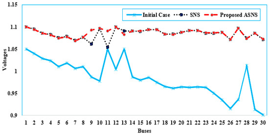
Figure 4. Voltage Profile of the proposed ASNS and SNS for Case 1 of the IEEE 30-bus grid.

In the second case, the minimization of TVD is considered where the SNS and proposed ASNS algorithms are executed, and the optimal control variables are shown in Table 3. The basic SNS algorithm reduces TVD from 0.8691 p.u. to 0.0846 p.u. when compared to the initial case; however, the proposed ASNS algorithm achieves the lowest TVD value of 0.08435 p.u. when compared to 0.8691 p.u. in the initial instance. This is a 90.3 percent reduction. The resulting solutions are contrasted with previously reported findings for minimizing the losses and utilizing the same circumstances, as summarized in Table 3, which shows that the proposed ASNS algorithm outperforms numerous strategies in minimizing the TGLs. LAO, ILAO [34], IPG-PSO [73], improved GSA [74], HFA [69], and QOTLBO achieved TVDs of 0.0945, 0.0876, 0.0892, 0.08968, 0.0980, and 0.0856, respectively.

Table 3. Optimal results for Case 2 of the IEEE 30-bus grid.

	Initial Case	SNS	Proposed ASNS	LAO * [34]	ILAO * [34]	IPG-PSO * [73]	Improved GSA * [74]	HFA * [69]	QOTLBO * [70]
VG 1	1.0500	1.0040	1.0041	1.0286	0.9942	1.0122	1.0085	1.0035	1.0005
VG 2	1.0400	1.0000	0.9999	0.9702	0.9563	1.0083	1.0057	1.0164	0.9919
VG 5	1.0100	1.0000	1.0000	1.0683	1.0689	1.0168	1.0192	1.0195	1.0217
VG 8	1.0100	1.0023	1.0033	0.9983	0.9919	1.0102	1.0103	1.0182	1.0147
VG 11	1.0500	1.0001	1.0000	1.0134	1.0650	1.0222	1.0184	0.9823	0.9950
VG 13	1.0500	1.0000	1.0001	1.0027	1.0436	1.0075	1.0079	1.0155	1.0447
Ta 6–9	1.0780	1.0074	1.0038	1.0100	1.0900	1.0390	1.0340	0.9900	1.0076
Ta 6–10	1.0690	1.0992	1.0814	0.9700	0.9400	0.9000	0.9000	0.9000	0.9030
Ta 4–12	1.0320	1.0196	1.0225	0.9700	1.0400	0.9759	0.9840	0.9800	1.0472
Ta 28–27	1.0680	0.9946	0.9816	0.9700	0.9800	0.9686	0.9780	0.9600	0.9674
Qr 10	0.0000	5.9271	12.0240	0.0000	0.0200	5.0000	5.0000	3.2000	4.8700
Qr 12	0.0000	12.6348	21.6595	2.0400	3.9900	1.8472	5.0000	0.5000	3.0400
Qr 15	0.0000	9.9277	3.9063	4.9900	4.5000	5.0000	5.0000	4.9000	5.0000
Qr 17	0.0000	9.3855	5.5190	0.3700	1.0800	0.0026	0.0000	0.1000	0.0000
Qr 20	0.0000	12.9420	12.6443	4.6400	4.6700	5.0000	5.0000	3.8000	5.0000
Qr 21	0.0000	16.4084	12.5312	0.0100	0.0200	5.0000	5.0000	5.0000	5.0000
Qr 23	0.0000	2.3579	3.3287	3.8800	4.9800	4.9915	5.0000	5.0000	5.0000
Qr 24	0.0000	12.3446	11.7143	4.0100	5.0000	4.9378	5.0000	3.9000	5.0000
Qr 29	0.0000	6.1102	3.8151	2.5300	4.7900	2.5206	4.9500	1.5000	2.5600
TGLs	5.7960	5.9001	5.7765	5.6154	6.2794	5.7429	5.7500	5.7500	6.4962
TVD	0.8691	0.0846	0.08435	0.0945	0.0876	0.0892	0.08968	0.0980	0.0856

* The techniques in the comparisons are not coded by the authors but are employed by their creators.

Furthermore, the convergent properties of the proposed ASNS and SNS for Case 2 of the IEEE 30-bus grid are depicted in Figure 5. As shown, the curve describes the minimization of the throughput of the iterations, while the small shape provides the range [0.08–0.2] p.u. The TVD starts at a high value of 1.4052 p.u. at the fifth iteration and continues decreasing, reaching 658, 0.1076, 0.09821, and 0.0856 p.u. at iterations 50, 100, 200, and 300, respectively.

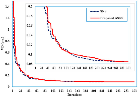
Figure 5. Convergence features of the proposed ASNS and SNS for Case 2 of the IEEE 30-bus grid.

Figure 6 depicts the voltage values acquired employing the proposed SNS and ASNS algorithms. As shown, the voltages employing the suggested SNS and ASNS are significantly better than in the initial case. Based on the suggested SNS and ASNS, the voltages at all buses are very close to the preferred flat voltage of 1 p.u.

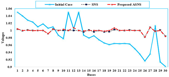
Figure 6. Voltage Profile of the proposed ASNS and SNS for Case 2 of the IEEE 30-bus grid.

In the third case, the minimization of VSI is considered where the SNS and ASNS algorithms are executed, and the optimal control variables are shown in Table 4. The basic SNS algorithm reduces VSI from 0.1720 p.u. to 0.1248 p.u. when compared to the initial case; however, the proposed ASNS algorithm achieves the lowest VSI index of 0.1243 p.u. when compared to 0.1720 p.u. in the initial instance. This is a 27.7 percent reduction.

Table 4. Optimal results for Case 3 of the IEEE 30-bus grid.

	Initial Case	SNS	Proposed ASNS
VG 1	1.0500	1.0990	1.0998
VG 2	1.0400	1.0933	1.0945
VG 5	1.0100	1.0671	1.1000
VG 8	1.0100	1.0869	1.1000
VG 11	1.0500	1.0998	1.0991
VG 13	1.0500	1.0997	1.0993
Ta 6–9	1.0780	0.9896	1.0351
Ta 6–10	1.0690	0.9355	0.9001
Ta 4–12	1.0320	1.0076	1.0315
Ta 28–27	1.0680	0.9545	0.9618
Qr 10	0.0000	5.5187	0.2385
Qr 12	0.0000	15.0421	18.0726
Qr 15	0.0000	0.4000	3.1113
Qr 17	0.0000	2.2772	8.5207
Qr 20	0.0000	5.4560	9.9379
Qr 21	0.0000	4.5358	2.0944
Qr 23	0.0000	7.4148	0.2498
Qr 24	0.0000	0.1587	0
Qr 29	0.0000	0.0183	0.0005
TGLs	5.7960	5.9001	4.9165
TVD	0.8691	2.7656	2.7286
VSI	0.1720	0.1248	0.1243

Table 5 compares the resulting solutions to previously reported findings in order to minimize the VSI objective. Furthermore, the convergent properties of the proposed ASNS and SNS for Case 3 of the IEEE 30-bus grid are depicted in Figure 7. As shown, the curve describes the minimization of the throughput of the iterations, while the small shape is provided on the range [0.1230–0.1480] p.u. The VSI starts at a high value of 0.1511 p.u. at the fifth iteration and continues decreasing, reaching 0.1259, 0.1249, and 0.1243 p.u. at iterations 100, 200, and 300, respectively.

Table 5. Comparative results for Case 3 of the IEEE 30-bus grid.

Method	VSI (p.u.)
Proposed ASNS	0.1243
SNS	0.1248
ABC * [44]	0.1280
GA * [75]	0.1807
SQP * [76]	0.1570
RGA * [76]	0.1386
CMAES * [76]	0.1382

* The techniques in the comparisons are not coded by the authors but are employed by their creators.

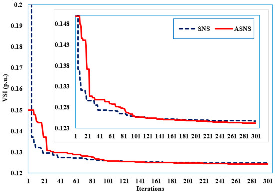
Figure 7. Convergence features of the proposed ASNS and SNS for Case 3 of the IEEE 30-bus grid.

As shown, the proposed ASNS algorithm outperforms numerous strategies in minimizing the VSI. ABC [44], GA [75], SQP, RGA, and CMAES [76] achieve VSIs of 0.1280, 0.1807, 0.1570, 0.1386, and 0.1382, respectively.

On the other side, taking into consideration the tap-changing transformers and shunt capacitors as discrete variables, Table 6 shows the corresponding results of the proposed ASNS algorithm for the three cases studied above. As shown, the outcomes are very similar. For the first case, the TGLs are minimized from 5.7960 to 4.5206 and 4.5222 MW, considering the continuous and discrete nature of tap-changing transformers and shunt capacitors. Furthermore, the TVD is minimized from 0.8691 to 0.08435 and 0.1037 p.u., while the VSI is minimized from 0.1720 to 0.1243 and 0.1241 p.u., respectively, considering the continuous and discrete nature of tap-changing transformers and shunt capacitors.

Table 6. Results for Cases 1–3 of the IEEE 30-bus grid considering the continuous and discrete nature of tap-changing transformers and shunt capacitors.

		Case 1 (TGLs Minimization)		Case 2 (TVD Minimization)		Case 3 (VSI Minimization)
	Initial Case	Continuous	Discrete	Continuous	Discrete	Continuous	Discrete
VG 1	1.0500	1.0999	1.0999	1.0041	1.0041	1.0998	1.0998
VG 2	1.0400	1.0941	1.0941	0.9999	0.9999	1.0945	1.0945
VG 5	1.0100	1.0741	1.0741	1.0000	1.1000	1.1000	1.1000
VG 8	1.0100	1.0759	1.0759	1.0033	1.0033	1.1000	1.1000
VG 11	1.0500	1.0907	1.0907	1.0000	1.1000	1.0991	1.0991
VG 13	1.0500	1.0824	1.0824	1.0001	1.0001	1.0993	1.0993
Ta 6–9	1.0780	0.9871	0.9800	1.0038	1.1000	1.0351	1.0400
Ta 6–10	1.0690	1.0185	1.0200	1.0814	1.0800	0.9001	0.9000
Ta 4–12	1.0320	0.9992	1.0000	1.0225	1.0300	1.0315	1.0300
Ta 28–27	1.0680	0.9669	0.9700	0.9816	0.9800	0.9618	0.9600
Qr 10	0.0000	11.8166	12.0000	12.0240	12.0000	0.2385	0.0000
Qr 12	0.0000	24.5761	25.0000	21.6595	22.0000	18.0726	18.0000
Qr 15	0.0000	3.7694	4.0000	3.9063	4.0000	3.1113	3.0000
Qr 17	0.0000	5.4730	5.0000	5.5190	6.0000	8.5207	9.0000
Qr 20	0.0000	3.5115	4.0000	12.6443	13.0000	9.9379	10.0000
Qr 21	0.0000	10.0785	10.0000	12.5312	13.0000	2.0944	2.0000
Qr 23	0.0000	1.3975	1.0000	3.3287	3.0000	0.2498	0.0000
Qr 24	0.0000	6.6386	7.0000	11.7143	12.0000	0.0000	0.0000
Qr 29	0.0000	2.1505	2.0000	3.8151	4.0000	0.0005	0.0000
TGLs	5.7960	4.5206	4.5222	5.7765	5.7884	4.9165	4.9185
TVD	0.8691	2.5863	2.5924	0.08435	0.1037	2.7286	2.7249
VSI	0.1720	0.1260	0.1264	0.1511	0.1506	0.1243	0.1241

4.2. Results of the Second Grid

The second grid comprises of 57-bus, 80-line, 7-generator and 15 on-load tap changing transformers, and 3 shunted compensators. The limits for the generator voltage and tap settings are 1.1000 and 0.9000 p.u., respectively. The minimum and maximum values for the shunt reactive power injections at buses 18, 25, and 53 are 10.0000, 5.9000, and 6.3000 MVAr, respectively.

In the first case, the SNS and proposed ASNS algorithms are implemented, and the best control settings are presented in Table 7. Furthermore, their convergent properties are depicted in Figure 8. The basic SNS algorithm reduces TGLs from 27.8640 MW to 23.9700 MW when compared to the initial case; however, the proposed ASNS algorithm achieves the lowest power losses of 23.8440 MW when compared to 27.8640 MW in the initial instance. This is a 14.42 % reduction.

Table 7. Optimal results for Cases 1–3 of the IEEE 57-bus grid.

		Case 1		Case 2		Case 3
	Initial Case	SNS	ASNS	SNS	ASNS	SNS	ASNS
VG 1	1.0400	1.0600	1.0600	1.0096	1.0093	1.0600	1.0398
VG 2	1.0100	1.0506	1.0508	1.0000	1.0001	1.0359	1.0266
VG 3	0.9850	1.0448	1.0451	1.0018	1.0021	1.0100	1.0202
VG 6	0.9800	1.0385	1.0405	1.0003	1.0004	0.9967	1.0234
VG 8	1.0050	1.0600	1.0600	1.0071	1.0038	1.0196	1.0392
VG 9	0.9800	1.0282	1.0287	0.9891	0.9876	1.0010	1.0108
VG 12	1.0150	1.0363	1.0351	1.0206	1.0214	1.0278	1.0406
Ta 4–18	0.9700	0.9001	1.0015	1.0124	0.9222	0.9042	0.9190
Ta 4–18	0.9780	1.0994	0.9264	0.9749	1.0603	0.9246	0.9900
Ta 21–20	1.0430	1.0357	1.0129	0.9808	0.9767	1.1000	1.0978
Ta 24–25	1.0000	1.0895	1.0221	1.0769	1.0806	0.9129	0.9001
Ta 24–25	1.0000	0.9340	1.0244	0.9922	1.0543	0.9412	1.0064
Ta 24–26	1.0430	0.9922	1.0070	0.9984	1.0007	1.0502	1.0629
Ta 7–29	0.9670	0.9538	0.9476	0.9951	0.9951	0.9134	0.9119
Ta 34–32	0.9750	0.9598	0.9612	0.9266	0.9165	0.9014	0.9000
Ta 11–41	0.9550	0.9002	0.9043	0.9016	0.9000	0.9007	0.9003
Ta 15–45	0.9550	0.9342	0.9335	0.9133	0.9190	0.9124	0.9223
Ta 14–46	0.9000	0.9294	0.9206	0.9628	0.9548	0.9003	0.9023
Ta 10–51	0.9300	0.9318	0.9282	0.9940	0.9974	0.9033	0.9141
Ta 13–49	0.8950	0.9113	0.9001	0.9000	0.9001	0.9272	0.9060
Ta 11–43	0.9580	0.9369	0.9175	0.9311	0.9407	0.9156	0.9038
Ta 40–56	0.9580	1.0019	1.0041	1.0093	0.9895	1.0397	1.0974
Ta 39–57	0.9800	0.9887	0.9733	0.9099	0.9025	0.9773	1.0901
Ta 9–55	0.9400	0.9424	0.9400	0.9902	0.9891	0.9580	0.9130
Qr 18	10.0000	22.4644	12.9690	11.8506	11.4394	10.6182	25.4222
Qr 25	5.9000	13.2932	14.9441	18.3588	20.0403	0.0006	0.2065
Qr 53	6.3000	12.5535	12.4807	28.6528	29.1235	22.3590	0.1518
TGLs	27.8640	23.9692	23.8441	28.3819	28.5729	26.1348	26.5536
TVD	1.3586	2.9201	3.4179	0.6520	0.6405	2.4676	2.9997
VSI	0.3000	0.2658	0.2604	0.2990	0.3031	0.2591	0.2542

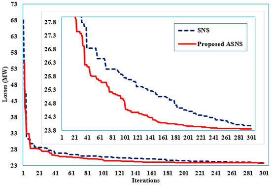
Figure 8. Convergence features of the proposed ASNS and SNS for Case 1 of the IEEE 57-bus grid.

The minimization of TVD is considered in the second case. Furthermore, the optimal control variables are shown in Table 7, while the convergent properties of the SNS and proposed ASNS algorithms are depicted in Figure 9. The basic SNS algorithm reduces TVD from 1.3586 p.u. to 0.6520 p.u. when compared to the initial case; however, the proposed ASNS algorithm achieves the lowest TVD of 0.6400 p.u. when compared to 1.3586 p.u. in the initial instance. This is a 52.85 percent reduction. For this case, Figure 10 depicts the voltage values acquired employing the proposed SNS and ASNS algorithms. As shown, there have been great improvements in the voltages based on the SNS and ASNS, where the voltages at all buses are very close to the preferred flat voltage of 1.0000 p.u. In addition, the minimum voltage of 0.9359 p.u. at bus 31 is greatly enhanced to be 1.0000 and 0.9800 p.u. based on the SNS and ASNS algorithms, respectively.

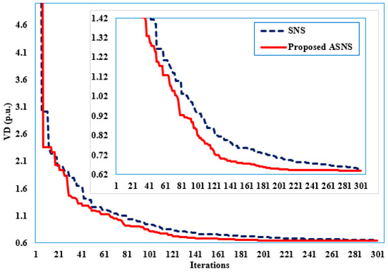
Figure 9. Convergence features of the proposed ASNS and SNS for Case 2 of the IEEE 57-bus grid.

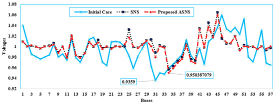
Figure 10. Voltage Profile of the proposed ASNS and SNS for Case 2 of the IEEE 57-bus grid.

The minimization of VSI is considered in the third case. Furthermore, the optimal control variables are shown in Table 7, while the convergent properties of the SNS and proposed ASNS algorithms are depicted in Figure 11. The basic SNS algorithm reduces VSI from 0.3000 p.u. to 0.2591 p.u. when compared to the initial case; however, the proposed ASNS algorithm achieves the lowest VSI of 0.2542 p.u. when compared to 0.3000 p.u. in the initial instance, with a reduction of 15.33%.

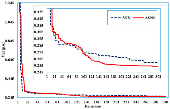
Figure 11. Convergence features of the proposed ASNS and SNS for Case 3 of the IEEE 57-bus grid.

Table 8 illustrates a comparative result of the obtained objectives based on the SNS and ASNS algorithms and other reported findings of several recent algorithms. For the first case, the proposed ASNS obtains the lowest minimum, mean, and maximum TGLs of 23.8441, 23.9695, and 24.4367, respectively. This comparison derives the superior performance of the proposed ASNS against BSA [77], SCA [47], SMA [78], improved SMA [78], SOA [79], ABC [44], and PSO-ICA [26]. Despite the improved SMA [78], which provides the lowest standard deviation of 0.0617 , the maximum TGLs recorded by the proposed ASNS of 24.4367 MW are better than the best TGLs obtained by it with 24.5856 MW.

Table 8. Comparative results for Cases 1 and 2 of the IEEE 57-bus grid.

Case 1 (TGLs Minimization)
Method	Min	Mean	Max	Std
Proposed ASNS	23.8441	23.9695	24.4367	0.1119
SNS	23.9692	24.7606	26.1838	0.7348
BSA * [77]	25.3980	24.8382	24.3744	0.2960
SCA * [47]	24.0540	24.6940	25.5270	0.3450
SMA * [78]	24.9009	25.5487	26.0263	0.2346
Improved SMA * [78]	24.5856	24.7079	24.8927	0.0617
SOA * [79]	24.2655	-	-	-
ABC * [44]	24.1025	-	-	-
PSO-ICA * [26]	25.5856	-	-	-
Case 2 (TVD Minimization)
	Min	Mean	Max	Std
Proposed ASNS	0.6405	0.6653	0.7230	0.0208
SNS	0.6520	0.7018	0.8237	0.0408
OGSA * [80]	0.6982	-	-	-
GB-WCA * [30]	0.6501	-	-	-
WCA * [30]	0.6631	-	-	-
Case 3 (VSI Minimization)
	Min	Mean	Max	Std
Proposed ASNS	0.2542	0.2586	0.2680	0.0029
SNS	0.2591	0.2650	0.2714	0.0036
HBO * [81]	0.6291	-	-	-
Improved HBO * [81]	0.5085	-	-	-

* The techniques in the comparisons are not coded by the authors but are employed by their creators.

For the second case, the proposed ASNS obtains the lowest minimum, mean, and maximum TVD of 0.6405, 0.6653, and 0.7230, while the basic SNS achieves counterparts of 0.6520, 0.7018, and 0.8237, respectively. This comparison derives the superior performance of the proposed ASNS against the oppositional GSA (OGSA) [80], GB-WCA [30], and WCA [30], which acquire TVDs of 0.6982, 0.6501, and 0.6631, respectively. For the third case, the proposed ASNS obtains the lowest minimum, mean, and maximum VSIs of 0.2542, 0.2586, 0.2,680, and 0.0029, while the basic SNS achieves counterparts of 0.2591, 0.2650, 0.2714, and 0.0036, respectively. This comparison derives the superior performance of the proposed ASNS against HBO [81], and improved HBO [81] which acquire TVDs of 0.6291 and 0.5085, respectively.

4.3. Results of the Third Grid (Large-Scale Case Study)

The proposed SNS and ASNS optimizers are implemented to solve the ORPD problem for the large-scale IEEE 118-bus power grid, and to illustrate and appraise their competency in solving larger-scale ORPD challenges. The grid’s complete data can be obtained in [65]. In the first case, the SNS and proposed ASNS algorithms are implemented, and the best control settings are presented in Table 9. Furthermore, their convergent properties are depicted in Figure 12. The proposed ASNS algorithm successfully achieves the minimum TGL of 85.9111 MW, whereas the basic SNS algorithm reduces it to 87.3385 MW.

Table 9. Optimal results for Case 1 of the IEEE 118-bus grid.

Variable	SNS	ASNS	Variable	SNS	ASNS	Variable	SNS	ASNS
VG 1	0.9506	0.9424	VG 62	0.9679	0.9720	VG 113	0.9682	0.9708
VG 4	0.9809	0.9713	VG 65	1.0036	1.0597	VG 116	0.9963	1.0572
VG 6	0.9715	0.9623	VG 66	0.9983	0.9985	Ta 8	1.0466	1.0461
VG 8	1.0470	1.0478	VG 69	1.0111	1.0045	Ta 32	1.0758	1.0498
VG 10	1.0598	1.0598	VG 70	0.9683	0.9717	Ta 36	1.0589	1.0477
VG 12	0.9673	0.9592	VG 72	0.9659	0.9679	Ta 51	1.0330	1.0495
VG 15	0.9553	0.9562	VG 73	0.9658	0.9673	Ta 93	1.0057	1.0796
VG 18	0.9610	0.9578	VG 74	0.9562	0.9593	Ta 95	1.0310	1.0859
VG 19	0.9543	0.9543	VG 76	0.9404	0.9400	Ta 102	0.9728	1.0262
VG 24	0.9746	0.9899	VG 77	0.9738	0.9730	Ta 107	0.9306	1.0104
VG 25	1.0073	1.0202	VG 80	0.9860	0.9835	Ta 127	1.0020	1.0570
VG 26	1.0591	1.0600	VG 85	0.9584	0.9726	Qr 34	4.1112	6.0706
VG 27	0.9635	0.9713	VG 87	0.9491	0.9657	Qr 44	6.7088	1.7000
VG 31	0.9559	0.9589	VG 89	0.9730	0.9913	Qr 45	26.5882	29.9781
VG 32	0.9589	0.9679	VG 90	0.9511	0.9627	Qr 46	1.2823	20.4191
VG 34	0.9628	0.9547	VG 91	0.9517	0.9658	Qr 48	9.3371	14.3187
VG 36	0.9584	0.9498	VG 92	0.9583	0.9730	Qr 74	22.5637	29.9500
VG 40	0.9554	0.9496	VG 99	0.9677	0.9691	Qr 79	29.9349	29.9540
VG 42	0.9582	0.9545	VG 100	0.9688	0.9741	Qr 82	27.7066	28.6906
VG 46	0.9699	0.9721	VG 103	0.9631	0.9583	Qr 83	10.5665	12.9289
VG 49	0.9847	0.9841	VG 104	0.9529	0.9445	Qr 105	18.8040	29.4293
VG 54	0.9534	0.9491	VG 105	0.9522	0.9451	Qr 107	17.9742	27.4281
VG 55	0.9518	0.9474	VG 107	0.9497	0.9418	Qr 110	10.9274	20.1976
VG 56	0.9518	0.9480	VG 110	0.9554	0.9468	TGLs	87.3385	85.9111
VG 59	0.9692	0.9679	VG 111	0.9629	0.9533	TVD	4.5467	4.8383
VG 61	0.9710	0.9733	VG 112	0.9489	0.9400

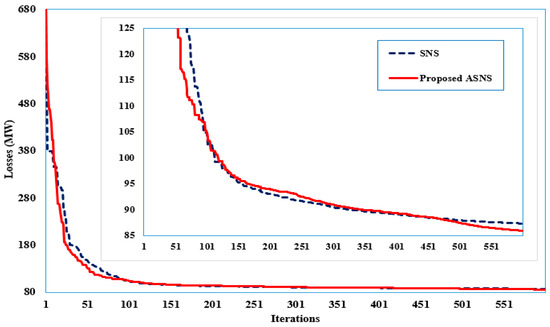
Figure 12. Convergence features of the proposed ASNS and SNS for Case 1 of the large-scale IEEE 118-bus grid.

For the second case, Table 10 illustrates a comparative result for the obtained objectives based on the SNS and ASNS algorithms and other reported findings of several recent algorithms. As shown, the proposed ASNS obtains the lowest minimum, mean, and maximum TGLs of 85.9111, 87.8445, and 89.7491 MW, respectively. This comparison derives the superior performance of the proposed ASNS against MPA [78], SMA [78], improved SMA [78], OGSA [80], GB-WCA [30], WCA [30], and PSO-ICA [26]. In the second case, the minimization of TVD is considered, and the optimal control variables are shown in Table 11, where the convergent properties of the SNS and proposed ASNS algorithms are depicted in Figure 13. The proposed ASNS algorithm successfully achieves the minimum TVD of 2.9878 p.u., whereas the basic SNS algorithm reduces it to 3.1799 p.u.

Table 10. Comparative results for Case 1 of the IEEE 118-bus grid.

Method	Min	Mean	Max	Std
Proposed ASNS	85.9111	87.8445	89.7491	1.0300
SNS	87.3385	89.0330	90.1690	0.6735
MPA * [78]	115.6104	117.2336	119.3328	1.0301
SMA * [78]	116.6795	118.0399	118.8109	0.5734
Improved SMA * [78]	114.7325	115.2126	115.6699	0.2520
OGSA * [80]	126.9900	-	-	-
GB-WCA * [30]	121.4700	-	-	-
WCA * [30]	131.8300	-	-	-
PSO-ICA * [26]	116.8550	-	-	-

* The techniques in the comparisons are not coded by the authors but are employed by their creators.

Table 11. Optimal results for Case 2 of the IEEE 118-bus grid.

Variable	SNS	ASNS	Variable	SNS	ASNS	Variable	SNS	ASNS
VG 1	0.9817	0.9813	VG 62	0.9580	0.9542	VG 113	0.9970	0.9575
VG 4	0.9978	1.0008	VG 65	0.9912	0.9660	VG 116	0.9558	0.9770
VG 6	0.9958	0.9998	VG 66	0.9925	0.9766	Ta 8	0.9180	0.9664
VG 8	0.9911	0.9999	VG 69	0.9995	1.0002	Ta 32	0.9899	1.0290
VG 10	0.9984	0.9997	VG 70	0.9786	0.9878	Ta 36	1.0241	0.9283
VG 12	0.9973	1.0000	VG 72	1.0026	1.0017	Ta 51	1.0331	1.0032
VG 15	0.9541	0.9568	VG 73	1.0024	1.0001	Ta 93	1.0512	0.9707
VG 18	0.9463	0.9508	VG 74	0.9551	0.9606	Ta 95	1.0378	0.9477
VG 19	0.9443	0.9485	VG 76	0.9405	0.9513	Ta 102	0.9966	0.9811
VG 24	1.0074	1.0030	VG 77	0.9833	0.9938	Ta 107	0.9489	0.9339
VG 25	1.0008	1.0048	VG 80	1.0096	1.0187	Ta 127	1.0156	1.0137
VG 26	0.9876	0.9878	VG 85	0.9644	0.9740	Qr 34	2.3968	8.3187
VG 27	0.9833	1.0096	VG 87	0.9998	1.0012	Qr 44	27.2772	23.1574
VG 31	1.0044	1.0019	VG 89	0.9609	0.9661	Qr 45	28.9069	29.6803
VG 32	0.9862	0.9965	VG 90	1.0034	1.0009	Qr 46	4.6377	28.9136
VG 34	0.9545	0.9591	VG 91	0.9544	0.9503	Qr 48	5.1663	16.6178
VG 36	0.9483	0.9522	VG 92	0.9504	0.9552	Qr 74	12.7093	9.0686
VG 40	0.9890	0.9990	VG 99	0.9905	1.0002	Qr 79	20.9656	26.9882
VG 42	1.0040	0.9979	VG 100	0.9597	0.9668	Qr 82	24.6778	29.6204
VG 46	1.0002	1.0131	VG 103	0.9552	0.9665	Qr 83	27.8694	29.0008
VG 49	1.0072	0.9941	VG 104	0.9483	0.9537	Qr 105	9.6319	0.1302
VG 54	0.9524	0.9533	VG 105	0.9534	0.9548	Qr 107	7.2698	14.0471
VG 55	0.9464	0.9506	VG 107	0.9983	1.0017	Qr 110	14.8929	26.5572
VG 56	0.9493	0.9507	VG 110	0.9483	0.9659	TGLs	100.0307	99.9273
VG 59	0.9604	0.9552	VG 111	0.9490	0.9589	TVD	3.1799	2.9878
VG 61	0.9611	0.9596	VG 112	0.9560	0.9794

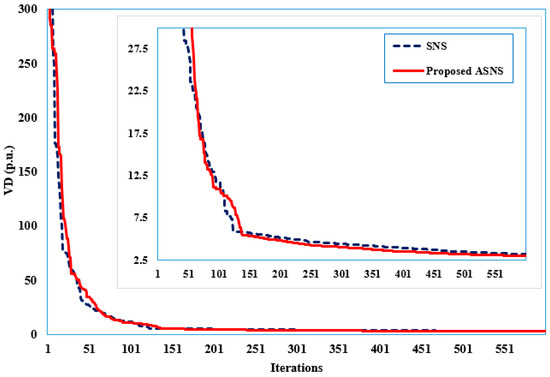
Figure 13. Convergence features of the ASNS and SNS for Case 2 of IEEE 118-bus grid.

The minimization of VSI is considered in the second case. Furthermore, the optimal control variables are shown in Table 12, while the convergent properties of the SNS and proposed ASNS algorithms are depicted in Figure 14. The proposed ASNS algorithm successfully achieves the minimum VSI of 0.0620 p.u., where the basic SNS algorithm reduces it to 0.0645 p.u.

Table 12. Optimal results for Case 3 of the IEEE 118-bus grid.

Variable	SNS	ASNS	Variable	SNS	ASNS	Variable	SNS	ASNS
VG 1	0.9402	0.9402	VG 62	0.9506	0.9408	VG 113	0.9477	0.9658
VG 4	0.9652	0.9806	VG 65	0.9521	0.9802	VG 116	0.9405	0.9453
VG 6	0.9670	0.9593	VG 66	0.9920	0.9648	Ta 8	0.9208	0.9000
VG 8	0.9572	0.9400	VG 69	1.0571	1.0544	Ta 32	0.9891	1.0238
VG 10	1.0040	0.9866	VG 70	0.9813	0.9749	Ta 36	0.9116	0.9758
VG 12	0.9637	0.9553	VG 72	0.9408	0.9474	Ta 51	0.9338	0.9004
VG 15	0.9446	0.9463	VG 73	0.9582	0.9427	Ta 93	0.9425	0.9352
VG 18	0.9516	0.9429	VG 74	0.9673	0.9569	Ta 95	0.9648	0.9470
VG 19	0.9413	0.9428	VG 76	0.9408	0.9400	Ta 102	0.9721	1.1000
VG 24	0.9461	0.9778	VG 77	0.9611	0.9628	Ta 107	0.9031	0.9202
VG 25	0.9746	0.9471	VG 80	0.9591	0.9627	Ta 127	0.9231	0.9042
VG 26	0.9726	0.9542	VG 85	0.9403	0.9404	Qr 34	2.2060	25.8409
VG 27	0.9576	0.9731	VG 87	0.9626	0.9533	Qr 44	29.9001	29.9736
VG 31	0.9427	0.9457	VG 89	0.9551	0.9564	Qr 45	29.6673	29.9865
VG 32	0.9400	0.9565	VG 90	0.9468	0.9410	Qr 46	3.7885	3.6437
VG 34	0.9516	1.0280	VG 91	0.9476	0.9561	Qr 48	3.3209	28.1680
VG 36	0.9443	1.0238	VG 92	0.9443	0.9433	Qr 74	18.1443	14.3624
VG 40	0.9400	1.0403	VG 99	0.9679	0.9400	Qr 79	24.6361	29.8855
VG 42	1.0600	1.0484	VG 100	0.9621	0.9513	Qr 82	23.6569	27.7690
VG 46	1.0600	1.0591	VG 103	0.9496	0.9560	Qr 83	4.1180	0.3922
VG 49	1.0394	1.0311	VG 104	0.9407	0.9400	Qr 105	19.6368	3.2235
VG 54	0.9482	0.9423	VG 105	0.9403	0.9451	Qr 107	16.2616	22.6529
VG 55	0.9451	0.9400	VG 107	0.9554	0.9774	Qr 110	0.2012	5.5425
VG 56	0.9466	0.9419	VG 110	0.9430	0.9474	TGLs	107.2403	106.9493
VG 59	0.9401	0.9414	VG 111	0.9568	0.9403	TVD	5.8744	5.7535
VG 61	0.9545	0.9471	VG 112	0.9401	0.9589	VSI	0.0645	0.0620

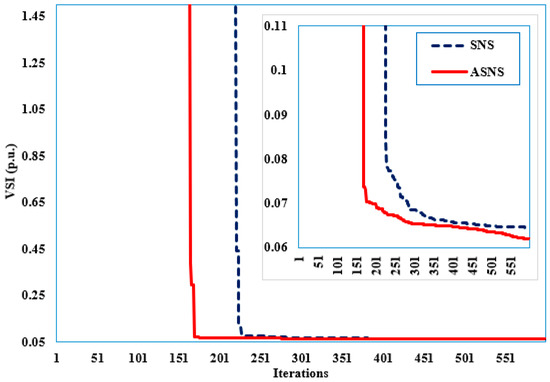
Figure 14. Convergence features of the proposed ASNS and SNS for Case 3 of the IEEE 118-bus grid.

4.4. SNS versus Proposed ASNS: Statistical Comparisons

To justify the rate of convergence of the proposed ASNS, the computational times (CPU times) of the SNS and ASNS are tabulated for the IEEE 30-, 57-, and 118-bus systems in Table 13. As shown, there is no significant difference between the SNS and ASNS in the computation time when solving the ORPD problem. In addition, the validation of the generators’ reactive power is demonstrated for IEEE 30-, 57-, and 118-bus systems, as stated in Appendix A.

Table 13. Average computational time per iteration using ASNS and SNS.

	SNS	Proposed ASNS
IEEE 30-bus systems	0.7222	0.6690
IEEE 57-bus systems	2.1332	2.1979
IEEE 118-bus systems	4.031	4.1401

For the sake of assessing the robustness study, the acquired minimum values of the TGLs and TVDs of the 30-runs are analyzed using the SNS and the proposed ASNS algorithms. Their spread and centers for both cases studied of the IEEE 30-, IEEE 57-, and IEEE 118-bus grids are described in Figure 15 via a Box and Whiskers plot. Furthermore, Table 14 displays the detailed robustness indices for Cases 1–3 of the IEEE 30-bus grid, and the percentage of improvement is evaluated to illustrate the difference between the results achieved by using SNS and ASNS regarding the medium-test system IEEE 30. Additionally, Figure 16 describes the obtained fitness values for both cases for the large-scale IEEE 118-bus grid. To investigate the analysis of the SNS and ASNS in terms of average success rate and convergence characteristics, minimizing the losses (Case 1) for the IEEEE 30-bus system is considered. At various percentages of convergence, including 70, 80, 90, and 100%, the absolute difference between the best and worst, its percentage, and the success rate are computed. Table 15 tabulates the related absolute difference between the best and worst and the best percentage, while Figure 17 depicts the regarded success rate. To investigate the robustness of the proposed algorithm parameters on the system behavior, the algorithm parameters are varied in terms of the number of search individuals and the maximum number of iterations, and the success rate is computed for minimizing the losses (Case 1) for the IEEE 30-bus system. The results are tabulated in Table 16.

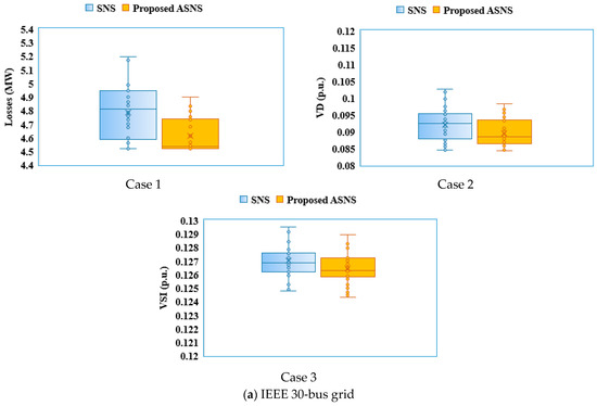
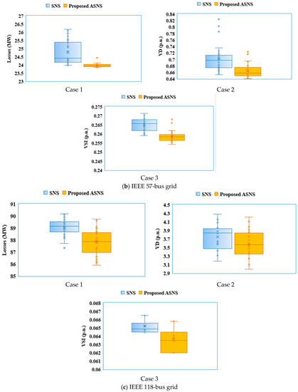
Figure 15. Box and Whiskers plot for the SNS and proposed ASNS of the IEEE 30-, IEEE 57-, and IEEE 118-bus grids.

Table 14. Detailed robustness indices for Cases 1-3 of the IEEE 30-bus grid.

	SNS	Proposed ASNS	% Improve	SNS	Proposed ASNS	% Improve	SNS	Proposed ASNS	% Improve
Min.	4.5208	4.5206	0.0036	0.084611	0.08435	0.3085	0.0652	0.0637	2.1955
Mean	4.7870	4.6154	3.5852	0.092111	0.089639	2.6837	0.0665	0.0658	1.0783
Max.	5.1931	4.8988	5.6675	0.102589	0.098258	4.2217	0.2714	0.2679	1.2360
Standard deviation	0.1916	0.1254	34.5600	0.0050	0.0041	18.7139	0.0036	0.0029	17.3804

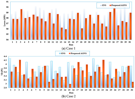
Figure 16. Obtained fitness values for SNS and proposed ASNS of the IEEE 118-bus grids.

Table 15. Absolute difference between the best and worst of SNS and ASNS for minimizing the losses (Case 1) for the IEEE 30-bus system.

	At 100% Convergence		At 90% Convergence		At 80% Convergence		At 70% Convergence
	SNS	ASNS	SNS	ASNS	SNS	ASNS	SNS	ASNS
|Best-worst| (MW)	0.6723	0.3781	0.6991	0.4451	0.7427	0.5441	0.7828	0.6340
|Best-worst| (%)	14.8700	8.3600	15.4600	10.0400	16.4300	12.0400	17.3100	14.0800

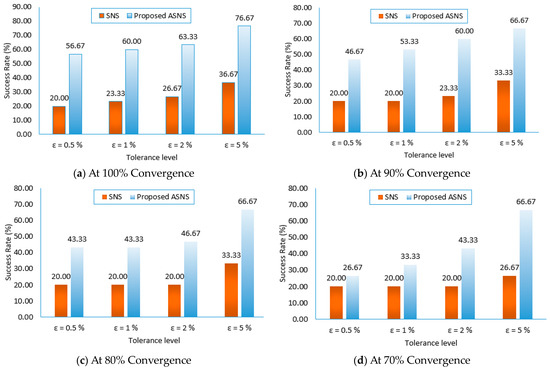
Figure 17. Success rates of SNS and ASNS for Case 1 for the IEEE 30-bus system.

Table 16. Success rates for different values of the ASNS parameters used for minimizing the losses (Case 1) for the IEEE 30-bus system.

Items and Values		Number of Search Individuals
		15	25	40	50
Maximum number of iterations	150	0.0000%	10.0000%	16.6667%	20.0000%
	200	3.3334%	16.6667%	16.6667%	33.3334%
	250	3.3334%	16.6667%	20.0000%	56.6667%
	300	6.6667%	16.6667%	26.6667%	76.6667%

Moreover, the effectiveness and performance of the envisaged ASNS and SNS are explored on 25 benchmark functions classified into unimodal, multimodal, fixed, and variable-dimension benchmark functions. Table 17 tabulates their full data in terms of their names, variable lengths, and permissible experiment intervals. The number of search individuals is 30 for the SNS and improved ASNS algorithms, and the maximum number of iterations is 1000. The simulations are performed thirty times. For this purpose, Table 17 provides detailed comparisons in terms of the mean, best, and standard deviation using ASNS and SNS as benchmark functions.

Table 17. Comparisons of the mean, best, and standard deviation using ASNS and SNS for benchmark functions.

Fun. No.	Name	Ranges	Dim.	Mean		Standard Deviation		Best
				ASNS	SNS	ASNS	SNS	ASNS	SNS
F1	Beale	[−4.5, 4.5]	2	0	0	0.0000	0.0000	0	0
F2	Schaffer No. 4	[−100, 100]	2	0.292579	0.292579	6.9100 × 10−17	6.9100 × 10−17	0.292579	0.292579
F3	Salomon	[−100, 100]	30	0.099873	0.099873	7.7500 × 10−14	1.9300 × 10−9	0.099873	0.099873
F4	Leon	[−1.2, 1.2]	2	0	1.16 × 10−26	0.0000	5.4100 × 10−26	0	1.23 × 10−32
F5	Zettl	[−5, 10]	2	−0.00172	−0.00224	1.0670 × 10−3	1.0970 × 10−3	−0.00351	−0.00377
F6	Sphere	[−100, 100]	30	3.0079 × 10−160	1.1789 × 10−147	9.5051 × 10−160	5.7805 × 10−147	7.1727 × 10−167	2.9501 × 10−152
F7	Schwefel’s 2.20	[−100, 100]	30	1.40367 × 10−81	2.58878 × 10−75	2.3913 × 10−81	6.4732 × 10−75	3.98714 × 10−83	2.44512 × 10−77
F8	Brown	[−1, 4]	30	2.6755 × 10−163	1.4484 × 10−151	0.0000	3.9041 × 10−151	1.3097 × 10−167	4.2958 × 10−156
F9	Powell Singular	[−4, 5]	30	1.69066 × 10−20	3.93264 × 10−10	8.7726 × 10−20	2.1540 × 10−9	4.43765 × 10−30	1.82433 × 10−38
F10	Perm 0,D,Beta	[−5, 5]	5	0.062787588	0.111982376	0.086737	0.16016	0.002908003	0.001297683
F11	Sum Squares	[−10, 10]	30	6.4142 × 10−161	1.1355 × 10−149	2.1289 × 10−160	2.5163 × 10−149	1.4778 × 10−165	2.6613 × 10−152
F12	Adjiman	[−1, 2]	2	−1.81123	−1.80019	0.18895	0.20109	−2.02181	−2.0201
F13	Bird	[−2pi, 2pi]	2	−82.1769	−75.2806	20.711	21.134	−106.193	−106.656
F14	Hartman 3	[0, 1]	3	−3.43303	−3.41297	0.27033	0.33938	−3.85014	−3.84113
F15	Cross-in-tray	[−10, 10]	2	−2.01815	−2.01409	0.046780	0.052864	−2.06206	−2.06043
F16	Cross leg table	[−10, 10]	2	−0.00011	−0.00011	1.4600 × 10−5	1.4900 × 10−5	−0.00014	−0.00015
F17	Crowned cross	[−10, 10]	2	0.001192	0.001317	1.6300 × 10−5	7.0700 × 10−4	0.00118	0.001177
F18	Helical Valley	[−10, 10]	3	6.69 × 10−82	5.79 × 10−46	2.5500 × 10−81	3.1700 × 10−45	6.96 × 10−91	1.61 × 10−64
F19	Shubert	[−10, 10]	2	−88.996	−77.3831	41.2951	44.065	−177.796	−179.212
F20	Periodic	[−10, 10]	30	1.044367	1.43648	0.053020	0.081863	1.001063	1.266691
F21	Qing	[−500, 500]	30	1.177906	5.138242	1.4770	13.791	0.103473	0.066978
F22	Alpine N. 1	[−10, 10]	30	1.83 × 10−83	2.46 × 10−77	2.5400 × 10−83	6.8600 × 10−77	1.26 × 10−85	4.67 × 10−79
F23	Xin-She Yang	[−5, 5]	30	1.79 × 10−75	2.44 × 10−54	9.6700 × 10−75	1.3400 × 10−53	8.23 × 10−94	6.89 × 10−72
F24	Wayburn Seader 3	[−500, 500]	2	19.10588	19.10588	1.4800 × 10−14	1.7800 × 10−14	19.10588	19.10588
F25	Dixon and Price	[−10, 10]	30	0.666666677	0.666666692	2.0899 × 10−8	4.7866 × 10−8	0.666666667	0.666666667

4.5. Discussion Analysis

The proposed ASNS and the original SNS algorithms derive adequate validation of the practical constraints related to the generators’ reactive power, which is demonstrated for IEEE 30-, 57-, and 118-bus systems. Based on the statistical comparisons via Figure 15, the proposed ASNS algorithm shows superior performance compared to the SNS algorithm for all cases studied of the IEEE 30-, IEEE 57-, and IEEE 118-bus grids.

For the IEEE 30-bus grid (Figure 15a), the proposed ASNS algorithm obtains the lowest minimum, mean, and maximum TGLs in the first case of 4.5207, 4.6154, and 4.8987 MW, respectively. Similarly, in the second case, it obtains the lowest minimum, mean, and maximum TVDs of 0.0843, 0.0896, and 0.0983 MW, respectively. Furthermore, the proposed ASNS algorithm provides the smallest standard deviations of TGLs of 0.1254 and TVD of 0.0041, respectively, relative to the SNS algorithm with TGLs of 0.1916 and TVD of 0.005.

As shown in Table 14, great improvement in the standard deviation is obtained with 34.5600, 18.7139, and 17.3804%, respectively, for Cases 1–3. Added to that, a great improvement in the maximum value is obtained with 5.6675, 4.2217, and 1.2360%, respectively, for Cases 1–3. Furthermore, significant improvements in the mean value are obtained with 3.5852, 2.6837, and 1.0783%, respectively, for Cases 1–3. For obtaining the minimum value, the obtained improvement is 0.0036, 0.3085, and 2.1955%, respectively, for Cases 1–3.

Similar findings are attained for the IEEE-57 bus grid (Figure 15b), where the proposed ASNS algorithm provides the smallest standard deviations of TGLs of 0.1119 and TVDs of 0.0207, respectively, relative to the SNS algorithm with TGLs of 0.7348 and TVDs of 0.0407.

For the IEEE 118-bus grid (Figure 15c), the proposed ASNS algorithm provides higher standard deviations of TGLs of 1.0300 and TVDs of 0.3300, respectively, relative to the SNS algorithm with TGLs of 0.6735 and TVDs of 0.3079. Despite that, the majority of the obtained fitness values for both cases are significantly lower than their counterparts using the SNS algorithm, as described in Figure 16.

From both Table 15 and Figure 17, the ASNS provides higher exploitation ability, which is increased with increasing the convergence level. It can be noted that:

• The proposed ASNS always achieves a lower difference percentage compared to the SNS. At 100% convergence, it has 8.36% while the SNS has 14.87%.
• The proposed ASNS always achieves a higher success rate compared to the SNS.
• At 90% and 100% convergence, the proposed ASNS provides approximately 2.5 times the success rate compared to the SNS. At 70% and 80% convergence, the ASNS provides approximately double the success rate of the SNS.

Furthermore, as shown in Table 16, increasing the maximum number of iterations increases the success rate. For example, at 50 search individuals, the success rate increases from 20% at 150 iterations to 33.33% at 200 iterations to 56.66% at 250 iterations to 76.66% at 300 iterations. Furthermore, the higher the number of search individuals, the higher the improvement of the success rate. For example, at 300 iterations, the success rate increased from 6.66% at 15 search individuals to 16.66% at 25 search individuals to 26.66% at 40 search individuals to 76.66% at 50 search individuals.

Nevertheless, higher robustness and effectiveness of the proposed improvements to the ASNS algorithm are demonstrated since the proposed ASNS successfully obtains the lowest mean, best, and standard deviation for the majority of the considered benchmark functions, as shown in Table 17.

4.6. Parameter Tuning of SNS and ASNS Algorithms

To demonstrate parameter tuning, the SNS and ASNS algorithms are used with varying numbers of search agents and iterations while power loss minimization is considered. At first, the IEEE 30-bus system is simulated, and Figure 18 describes the corresponding curves for both algorithms.

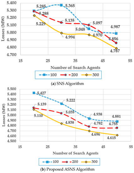
Figure 18. Parameter Tuning of SNS and ASNS Algorithms for Case 1 for the IEEE 30-bus system.

As shown, the lowest power losses are achieved at 50 search agents and 300 iterations for both algorithms. Therefore, the SNS and ASNS algorithms are set to have these characteristics as stated in Table A1 in Appendix A. Furthermore, for both algorithms, increasing the number of iterations and the search agents results in reduced power losses. The proposed ASNS algorithm shows great superiority compared to the original SNS for most of the combinations of the iterations and the search agents. For example, at 300 iterations, the proposed ASNS algorithm provides a reduction in power losses of 2.29, 3.11, 5.51, and 3.59% at a number of search agents of 20, 30, 40, and 50, respectively.

Furthermore, the IEEE 57-bus system is simulated, and Figure 19 depicts the relevant contours for both methods. As demonstrated, the suggested ASNS algorithm outperforms the original SNS for the majority of cycles and search agent combinations. At 100 rounds, the suggested ASNS algorithm reduces power losses by 2.29, 3.71, 4.28, and 4.76% at search agent counts of 30, 40, and 50, respectively. At 200 rounds, the suggested ASNS algorithm reduces power losses by 4.36, 5.76, and 4.83% at search agent counts of 30, 40, and 50, respectively. At 300 rounds, the suggested ASNS algorithm improves power losses by 3.97, 3.95, and 3.19% at search agent counts of 30, 40, and 50, respectively.

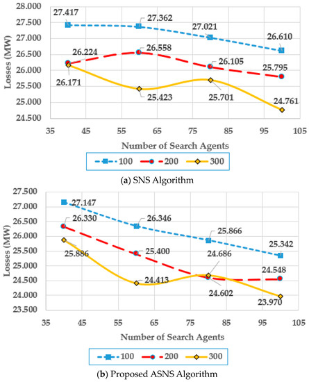
Figure 19. Parameter Tuning of SNS and ASNS Algorithms for Case 1 for IEEE 57-bus system.

Furthermore, for both algorithms, increasing the number of iterations and search agents results in a greater decrease in power losses. Both methods attain the lowest power losses at 100 search agents and 300 iterations. As a result, the SNS and ASNS algorithms are configured to have the traits listed in Table A1 in Appendix A.

Finally, the IEEE 118-bus system is simulated, and Figure 20 describes the corresponding curves for both algorithms.

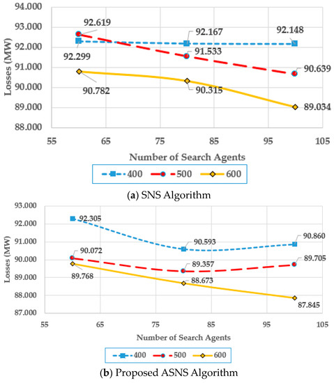
Figure 20. Parameter Tuning of SNS and ASNS Algorithms for Case 1 for the IEEE 118-bus system.

As demonstrated, the suggested ASNS algorithm outperforms the original SNS for most of the repetition and search agent combinations. For example, at 600 iterations, the proposed ASNS algorithm provides a reduction in power losses of 1.12, 1.82, and 1.34% at a number of search agents of 60, 80, and 100, respectively. Furthermore, for both algorithms, increasing the number of iterations and search agents results in a greater decrease in power losses. Both algorithms attain the lowest power losses at 100 search agents and 600 rounds. Therefore, the SNS and ASNS algorithms are set to have these characteristics as stated in Table A1 in Appendix A.

5. Conclusions

This study introduces an intelligent optimizer used for finding the optimal scheduling of reactive ORPD power resources (i.e., ASNS). ASNS aims to reduce real power losses and voltage variations while avoiding falling into local optima through two strategies: effective exploitation and adaptable parameter strategies. Simulations were conducted using three standard grids, the IEEE 30-, 57-, and 118-bus. The performance validation across companies’ diverse comparisons and statistical analyses is compared with the state of the art. The proposed analysis demonstrates the capability of the ASNS to tackle the ORPD issues with effective and robust performance. The proposed ASNS shows superiority over the state of the art and achieves a great reduction of power losses ( 22%, 14.42%, and 1.62%) and a higher improvement of voltage profiles of 90.3%, 52.85%, and 6.07% for IEEE 30-, IEEE 57-, and IEEE 118-bus grids, respectively. Furthermore, the simulation results show that the ASNS algorithm supports the diversity of populations.

The main objectives that are usually utilized in the ORPD problem are power loss, voltage profile, and voltage stability. Usually, they are very important measures that reflect the technical performance of the steady state operating condition of the system under study. On the other side, some other objectives could be considered for future work, such as reactive power reserve margin maximization and loadability enhancement. Therefore, the future of this study covers two categories. The first aims to solve other complex problems such as OPF for different power system requirements, adding new constraints and limitations for AC/DC grids with the high penetration of renewable energy resources. On the other hand, from the standpoint of solution methodology, developing other optimization algorithms to solve the considered problems.

References

- Chen, X.; Li, K.; Xu, B.; Yang, Z. Biogeography-based learning particle swarm optimization for combined heat and power economic dispatch problem. Knowl.-Based Syst. 2020, 208, 106463. [Google Scholar] [CrossRef]
- Acharya, S.; Ganesan, S.; Kumar, D.V.; Subramanian, S. A multi-objective multi-verse optimization algorithm for dynamic load dispatch problems. Knowl.-Based Syst. 2021, 231, 107411. [Google Scholar] [CrossRef]
- Naderi, E.; Narimani, H.; Pourakbari-Kasmaei, M.; Cerna, F.V.; Marzband, M.; Lehtonen, M. State-of-the-Art of Optimal Active and Reactive Power Flow: A Comprehensive Review from Various Standpoints. Processes 2021, 9, 1319. [Google Scholar] [CrossRef]
- Bentouati, B.; Khelifi, A.; Shaheen, A.M.; El-Sehiemy, R.A. An enhanced moth-swarm algorithm for efficient energy management based multi dimensions OPF problem. J. Ambient Intell. Humaniz. Comput. 2020, 12, 1–21. [Google Scholar] [CrossRef]
- Muhammad, Y.; Khan, R.; Raja, M.A.Z.; Ullah, F.; Chaudhary, N.I.; He, Y. Solution of optimal reactive power dispatch with FACTS devices: A survey. Energy Rep. 2020, 6, 2211–2229. [Google Scholar] [CrossRef]
- Rezaie, H.; Kazemi-Rahbar, M.H.; Vahidi, B.; Rastegar, H. Solution of combined economic and emission dispatch problem using a novel chaotic improved harmony search algorithm. J. Comput. Des. Eng. 2019, 6, 447–467. [Google Scholar] [CrossRef]
- Roy, P.K.; Ghoshal, S.P.; Thakur, S.S. Biogeography based optimization for multi-constraint optimal power flow with emission and non-smooth cost function. Expert Syst. Appl. 2010, 37, 8221–8228. [Google Scholar] [CrossRef]
- Hassan, M.H.; Kamel, S.; Abualigah, L.; Eid, A. Development and application of slime mould algorithm for optimal economic emission dispatch. Expert Syst. Appl. 2021, 182, 115205. [Google Scholar] [CrossRef]
- Bhadoria, A.; Marwaha, S. Moth flame optimizer-based solution approach for unit commitment and generation scheduling problem of electric power system. J. Comput. Des. Eng. 2020, 7, 668–683. [Google Scholar] [CrossRef]
- Shaheen, A.; Ginidi, A.; El-Sehiemy, R.; Elsayed, A.; Elattar, E.; Dorrah, H.T. Developed Gorilla Troops Technique for Optimal Power Flow Problem in Electrical Power Systems. Mathematics 2022, 10, 1636. [Google Scholar] [CrossRef]
- Lujano-Rojas, J.M.; Zubi, G.; Dufo-Lopez, R.; Bernal-Agustin, J.L.; Atencio-Guerra, J.L.; Catalao, J.P.S. Embedding quasi-static time series within a genetic algorithm for stochastic optimization: The case of reactive power compensation on distribution systems. J. Comput. Des. Eng. 2020, 7, 177–194. [Google Scholar] [CrossRef]
- Deeb, N.I.; Shahidehpour, S.M. An Efficient Technique for Reactive Power Dispatch Using a Revised Linear Programming Approach. Electr. Power Syst. Res. 1988, 15, 121–134. [Google Scholar] [CrossRef]
- Venkatesh, S.V.; Liu, W.H.E.; Papalexopoulos, A.D. A Least Squares Solution for Optimal Power Flow Sensitivity Calculation. IEEE Trans. Power Syst. 1992, 7, 1394–1401. [Google Scholar] [CrossRef]
- Quintana, V.H.; Santos-Nieto, M. Reactive-power dispatch by successive quadratic programming. IEEE Trans. Energy Convers. 1989, 4, 425–435. [Google Scholar] [CrossRef]
- Granville, S. Opiimal reactive dispatch through interior point methods. IEEE Trans. Power Syst. 1994, 9, 136–146. [Google Scholar] [CrossRef]
- El-Sehiemy, R.A.; El Ela, A.A.A.; Shaheen, A. A multi-objective fuzzy-based procedure for reactive power-based preventive emergency strategy. Int. J. Eng. Res. Afr. 2015, 13, 91–102. [Google Scholar] [CrossRef]
- Vlachogiannis, J.G.; Lee, K.Y. Quantum-inspired evolutionary algorithm for real and reactive power dispatch. IEEE Trans. Power Syst. 2008, 23, 1627–1636. [Google Scholar] [CrossRef]
- Yoshida, H.; Kawata, K.; Fukuyama, Y.; Takayama, S.; Nakanishi, Y. A Particle swarm optimization for reactive power and voltage control considering voltage security assessment. IEEE Trans. Power Syst. 2000, 15, 1232–1239. [Google Scholar] [CrossRef]
- Esmin, A.A.A.; Lambert-Torres, G.; Zambroni de Souza, A.C. A hybrid particle swarm optimization applied to loss power minimization. IEEE Trans. Power Syst. 2005, 20, 859–866. [Google Scholar] [CrossRef]
- Tripathy, M.; Mishra, S. Bacteria foraging-based solution to optimize both real power loss and voltage stability limit. IEEE Trans. Power Syst. 2007, 22, 240–248. [Google Scholar] [CrossRef]
- Subbaraj, P.; Rajnarayanan, P.N. Optimal reactive power dispatch using self-adaptive real coded genetic algorithm. Electr. Power Syst. Res. 2009, 79, 374–381. [Google Scholar] [CrossRef]
- Mahadevan, K.; Kannan, P.S. Comprehensive learning particle swarm optimization for reactive power dispatch. Appl. Soft Comput. 2010, 10, 641–652. [Google Scholar] [CrossRef]
- Sivasubramani, S.; Swarup, K.S. Multi-objective harmony search algorithm for optimal power flow problem. Int. J. Electr. Power Energy Syst. 2011, 33, 745–752. [Google Scholar] [CrossRef]
- Duman, S.; Sönmez, Y.; Güvenç, U.; Yörükeren, N. Optimal reactive power dispatch using a gravitational search algorithm. IET Gener. Transm. Distrib. 2012, 6, 563–576. [Google Scholar] [CrossRef]
- Singh, H.; Srivastava, L. Modified Differential Evolution algorithm for multi-objective VAR management. Int. J. Electr. Power Energy Syst. 2014, 55, 731–740. [Google Scholar] [CrossRef]
- Mehdinejad, M.; Mohammadi-Ivatloo, B.; Dadashzadeh-Bonab, R.; Zare, K. Solution of optimal reactive power dispatch of power systems using hybrid particle swarm optimization and imperialist competitive algorithms. Int. J. Electr. Power Energy Syst. 2016, 83, 104–116. [Google Scholar] [CrossRef]
- Rajan, A.; Malakar, T. Exchange market algorithm based optimum reactive power dispatch. Appl. Soft Comput. 2016, 43, 320–336. [Google Scholar] [CrossRef]
- Mouassa, S.; Bouktir, T.; Salhi, A. Ant lion optimizer for solving optimal reactive power dispatch problem in power systems. Eng. Sci. Technol. an Int. J. 2017, 20, 885–895. [Google Scholar] [CrossRef]
- Li, Z.; Cao, Y.; Van Dai, L.; Yang, X.; Nguyen, T.T. Finding solutions for optimal reactive power dispatch problem by a novel improved antlion optimization algorithm. Energies 2019, 12, 2968. [Google Scholar] [CrossRef]
- Heidari, A.A.; Ali Abbaspour, R.; Rezaee Jordehi, A. Gaussian bare-bones water cycle algorithm for optimal reactive power dispatch in electrical power systems. Appl. Soft Comput. J. 2017, 57, 657–671. [Google Scholar] [CrossRef]
- Mouassa, S.; Bouktir, T. Multi-objective ant lion optimization algorithm to solve large-scale multi-objective optimal reactive power dispatch problem. COMPEL Int. J. Comput. Math. Electr. Electron. Eng. 2019, 38, 304–324. [Google Scholar] [CrossRef]
- Shareef, S.M.; Srinivasa Rao, R. Optimal reactive power dispatch under unbalanced conditions using hybrid swarm intelligence. Comput. Electr. Eng. 2018, 69, 183–193. [Google Scholar] [CrossRef]
- Lenin, K. Minimization of real power loss by enhanced teaching learning based optimization algorithm Corresponding Author. Int. J. Robot. Autom. 2020, 9, 1–5. [Google Scholar] [CrossRef]
- Ebeed, M.; Ali, A.; Mosaad, M.I.; Kamel, S. An improved lightning attachment procedure optimizer for optimal reactive power dispatch with uncertainty in renewable energy resources. IEEE Access 2020, 8, 168721–168731. [Google Scholar] [CrossRef]
- El-Sehiemy, R.A. A novel single/multi-objective frameworks for techno-economic operation in power systems using tunicate swarm optimization technique. J. Ambient Intell. Humaniz. Comput. 2022, 13, 1073–1091. [Google Scholar] [CrossRef]
- Mouassa, S.; Jurado, F.; Bouktir, T.; Raja, M.A.Z. Novel design of artificial ecosystem optimizer for large-scale optimal reactive power dispatch problem with application to Algerian electricity grid. Neural Comput. Appl. 2021, 33, 7467–7490. [Google Scholar] [CrossRef]
- Korashy, A.; Kamel, S.; Houssein, E.H.; Jurado, F.; Hashim, F.A. Development and Application of Evaporation Rate Water Cycle Algorithm for Optimal Coordination of Directional Overcurrent Relays. Expert Syst. Appl. 2021, 185, 115538. [Google Scholar] [CrossRef]
- Qian, J.; Wang, P.; Pu, C.; Chen, G. Joint application of multi-object beetle antennae search algorithm and BAS-BP fuel cost forecast network on optimal active power dispatch problems. Knowl.-Based Syst. 2021, 226, 107149. [Google Scholar] [CrossRef]
- Liang, R.H.; Wang, J.C.; Chen, Y.T.; Tseng, W.T. An enhanced firefly algorithm to multi-objective optimal active/reactive power dispatch with uncertainties consideration. Int. J. Electr. Power Energy Syst. 2015, 64, 1088–1097. [Google Scholar] [CrossRef]
- Basu, M. Multi-objective optimal reactive power dispatch using multi-objective differential evolution. Int. J. Electr. Power Energy Syst. 2016, 82, 213–224. [Google Scholar] [CrossRef]
- Robbins, B.A.; Domínguez-García, A.D. Optimal Reactive Power Dispatch for Voltage Regulation in Unbalanced Distribution Systems. IEEE Trans. Power Syst. 2016, 31, 2903–2913. [Google Scholar] [CrossRef]
- Basu, M. Quasi-oppositional differential evolution for optimal reactive power dispatch. Int. J. Electr. Power Energy Syst. 2016, 78, 29–40. [Google Scholar] [CrossRef]
- Nasouri Gilvaei, M.; Jafari, H.; Jabbari Ghadi, M.; Li, L. A novel hybrid optimization approach for reactive power dispatch problem considering voltage stability index. Eng. Appl. Artif. Intell. 2020, 96, 103963. [Google Scholar] [CrossRef]
- Ettappan, M.; Vimala, V.; Ramesh, S.; Kesavan, V.T. Optimal reactive power dispatch for real power loss minimization and voltage stability enhancement using Artificial Bee Colony Algorithm. Microprocess. Microsyst. 2020, 76, 103085. [Google Scholar] [CrossRef]
- Biswas, P.P.; Suganthan, P.N.; Mallipeddi, R.; Amaratunga, G.A.J. Optimal reactive power dispatch with uncertainties in load demand and renewable energy sources adopting scenario-based approach. Appl. Soft Comput. 2019, 75, 616–632. [Google Scholar] [CrossRef]
- Zhang, X.; Yu, T.; Yang, B.; Cheng, L. Accelerating bio-inspired optimizer with transfer reinforcement learning for reactive power optimization. Knowl.-Based Syst. 2017, 116, 26–38. [Google Scholar] [CrossRef]
- Saddique, M.S.; Bhatti, A.R.; Haroon, S.S.; Sattar, M.K.; Amin, S.; Sajjad, I.A.; ul Haq, S.S.; Awan, A.B.; Rasheed, N. Solution to optimal reactive power dispatch in transmission system using meta-heuristic techniques―Status and technological review. Electr. Power Syst. Res. 2020, 178, 106031. [Google Scholar] [CrossRef]
- ben oualid Medani, K.; Sayah, S.; Bekrar, A. Whale optimization algorithm based optimal reactive power dispatch: A case study of the Algerian power system. Electr. Power Syst. Res. 2018, 163, 696–705. [Google Scholar] [CrossRef]
- Suresh, V.; Kumar, S.S. Optimal reactive power dispatch for minimization of real power loss using SBDE and DE-strategy algorithm. J. Ambient Intell. Humaniz. Comput. 2020, 1–15. [Google Scholar] [CrossRef]
- Ebeed, M.; Alhejji, A.; Kamel, S.; Jurado, F. Solving the Optimal Reactive Power Dispatch Using Marine Predators Algorithm Considering the Uncertainties in Load and Wind-Solar Generation Systems. Energies 2020, 13, 4316. [Google Scholar] [CrossRef]
- Abd-El Wahab, A.M.; Kamel, S.; Hassan, M.H.; Mosaad, M.I.; AbdulFattah, T.A. Optimal Reactive Power Dispatch Using a Chaotic TurbulentFlow of Water-Based Optimization Algorithm. Mathematics 2022, 10, 346. [Google Scholar] [CrossRef]
- PG, A.K.; Devaraj, D. Hybrid CAC-DE in optimal reactive power dispatch (ORPD) for renewable energy cost reduction. Sustain. Comput. Inform. Syst. 2022, 35, 100688. [Google Scholar] [CrossRef]
- Kien, L.C.; Nguyen, T.T.; Pham, T.D.; Nguyen, T.T. Cost reduction for energy loss and capacitor investment in radial distribution networks applying novel algorithms. Neural Comput. Appl. 2021, 33, 15495–15522. [Google Scholar] [CrossRef]
- Mahfoud, R.J.; Alkayem, N.F.; Sun, Y.; Haes Alhelou, H.; Siano, P.; Parente, M. Improved hybridization of evolutionary algorithms with a sensitivity-based decision-making technique for the optimal planning of shunt capacitors in radial distribution systems. Appl. Sci. 2020, 10, 1384. [Google Scholar] [CrossRef]
- Jamil Mahfoud, R.; Sun, Y.; Faisal Alkayem, N.; Haes Alhelou, H.; Siano, P.; Shafie-khah, M. A novel combined evolutionary algorithm for optimal planning of distributed generators in radial distribution systems. Appl. Sci. 2019, 9, 3394. [Google Scholar] [CrossRef]
- Le Kien, C.; Tuyet, Y.; Thi, N.; Phan, T.M.; Nguyen, T.T. Finding Optimal Solutions for the Placement of Reactive and Active Power Generation Components in Distribution Networks Using a High-Performance Metaheuristic Algorithm. Int. Trans. Electr. Energy Syst. 2022, 2022, 3761983. [Google Scholar]
- Talatahari, S.; Bayzidi, H.; Saraee, M. Social Network Search for Global Optimization. IEEE Access 2021, 9, 92815–92863. [Google Scholar] [CrossRef]
- El-Sehiemy, R.; Elsayed, A.; Shaheen, A.; Elattar, E.; Ginidi, A. Scheduling of Generation Stations, OLTC Substation Transformers and VAR Sources for Sustainable Power System Operation Using SNS Optimizer. Sustainability 2021, 13, 11947. [Google Scholar] [CrossRef]
- Shaheen, A.M.; Elsayed, A.M.; Ginidi, A.R.; El-Sehiemy, R.A.; Elattar, E. Enhanced social network search algorithm with powerful exploitation strategy for PV parameters estimation. Energy Sci. Eng. 2022, 10, 1398–1417. [Google Scholar] [CrossRef]
- Shaheen, A.M.; El-Sehiemy, R.A.; Farrag, S.M. A novel framework for power loss minimization by modified wind driven optimization algorithm. In Proceedings of the 2018 International Conference on Innovative Trends in Computer Engineering, ITCE, Aswan, Egypt, 19–21 February 2018; IEEE: Piscataway, NJ, USA, 2018; Volume 2018. [Google Scholar]
- Shaheen, A.M.; Spea, S.R.; Farrag, S.M.; Abido, M.A. A review of meta-heuristic algorithms for reactive power planning problem. Ain Shams Eng. J. 2018, 9, 215–231. [Google Scholar] [CrossRef]
- Shaheen, A.M.; El-Sehiemy, R.A.; Farrag, S.M. Optimal reactive power dispatch using backtracking search algorithm. Aust. J. Electr. Electron. Eng. 2016, 13, 200–210. [Google Scholar] [CrossRef]
- Ginidi, A.R.; Elsayed, A.M.; Shaheen, A.M.; Elattar, E.E.; El-Sehiemy, R.A. A Novel Heap based Optimizer for Scheduling of Large-scale Combined Heat and Power Economic Dispatch. IEEE Access 2021, 9, 83695–83708. [Google Scholar] [CrossRef]
- Shaheen, A.M.; Elsayed, A.M.; Ginidi, A.R.; El-Sehiemy, R.A.; Elattar, E. A heap-based algorithm with deeper exploitative feature for optimal allocations of distributed generations with feeder reconfiguration in power distribution networks. Knowl.-Based Syst. 2022, 241, 108269. [Google Scholar] [CrossRef]
- Zimmerman, R.D.; Murillo-Sánchez, C.E.; Thomas, R.J. Matpower [Software]. Available online: https://matpower.org (accessed on 2 January 2023).
- Electric Grid Test Cases. Available online: https://electricgrids.engr.tamu.edu/electric-grid-test-cases/ (accessed on 2 January 2023).
- Elattar, E.E.; Shaheen, A.M.; Elsayed, A.M.; El-Sehiemy, R.A. Optimal power flow with emerged technologies of voltage source converter stations in meshed power systems. IEEE Access 2020, 8, 166963–166979. [Google Scholar] [CrossRef]
- Ghasemi, M.; Taghizadeh, M.; Ghavidel, S.; Aghaei, J.; Abbasian, A. Solving optimal reactive power dispatch problem using a novel teaching-learning-based optimization algorithm. Eng. Appl. Artif. Intell. 2015, 39, 100–108. [Google Scholar] [CrossRef]
- Rajan, A.; Malakar, T. Optimal reactive power dispatch using hybrid Nelder-Mead simplex based firefly algorithm. Int. J. Electr. Power Energy Syst. 2015, 66, 9–24. [Google Scholar] [CrossRef]
- Mandal, B.; Roy, P.K. Optimal reactive power dispatch using quasi-oppositional teaching learning based optimization. Int. J. Electr. Power Energy Syst. 2013, 53, 123–134. [Google Scholar] [CrossRef]
- Mei, R.N.S.; Sulaiman, M.H.; Mustaffa, Z.; Daniyal, H. Optimal reactive power dispatch solution by loss minimization using moth-flame optimization technique. Appl. Soft Comput. 2017, 59, 210–222. [Google Scholar]
- Shaheen, A.M.; El-Sehiemy, R.A.; Ginidi, A.R.; Ghoneim, S.S.M.; Alharthi, M.M. Multi-objective jellyfish search optimizer for efficient power system operation based on multi-dimensional OPF framework. Energy 2021, 237, 121478. [Google Scholar] [CrossRef]
- Polprasert, J.; Ongsakul, W.; Dieu, V.N. Optimal reactive power dispatch using improved pseudo-gradient search particle swarm optimization. Electr. Power Compon. Syst. 2016, 44, 518–532. [Google Scholar] [CrossRef]
- Chen, G.; Liu, L.; Zhang, Z.; Huang, S. Optimal reactive power dispatch by improved GSA-based algorithm with the novel strategies to handle constraints. Appl. Soft Comput. 2017, 50, 58–70. [Google Scholar] [CrossRef]
- Devaraj, D.; Roselyn, J.P. Genetic algorithm based reactive power dispatch for voltage stability improvement. Int. J. Electr. Power Energy Syst. 2010, 32, 1151–1156. [Google Scholar] [CrossRef]
- Jeyadevi, S.; Baskar, S.; Babulal, C.K.; Willjuice Iruthayarajan, M. Solving multiobjective optimal reactive power dispatch using modified NSGA-II. Int. J. Electr. Power Energy Syst. 2011, 33, 219–228. [Google Scholar] [CrossRef]
- Shaheen, A.M.; El-Sehiemy, R.A.; Farrag, S.M. Integrated Strategies of Backtracking Search Optimizer for Solving Reactive Power Dispatch Problem. IEEE Syst. J. 2018, 12, 424–433. [Google Scholar] [CrossRef]
- Wei, Y.; Zhou, Y.; Luo, Q.; Deng, W. Optimal reactive power dispatch using an improved slime mould algorithm. Energy Rep. 2021, 7, 8742–8759. [Google Scholar] [CrossRef]
- Dai, C.; Chen, W.; Zhu, Y.; Zhang, X. Seeker optimization algorithm for optimal reactive power dispatch. IEEE Trans. Power Syst. 2009, 24, 1218–1231. [Google Scholar]
- Shaw, B.; Mukherjee, V.; Ghoshal, S.P. Solution of reactive power dispatch of power systems by an opposition-based gravitational search algorithm. Int. J. Electr. Power Energy Syst. 2014, 55, 29–40. [Google Scholar] [CrossRef]
- Elsayed, S.K.; Kamel, S.; Selim, A.; Ahmed, M. An Improved Heap-Based Optimizer for Optimal Reactive Power Dispatch. IEEE Access 2021, 9, 58319–58336. [Google Scholar] [CrossRef]
Disclaimer/Publisher’s Note: The statements, opinions and data contained in all publications are solely those of the individual author(s) and contributor(s) and not of MDPI and/or the editor(s). MDPI and/or the editor(s) disclaim responsibility for any injury to people or property resulting from any ideas, methods, instructions or products referred to in the content. |
© 2023 by the authors. Licensee MDPI, Basel, Switzerland. This article is an open access article distributed under the terms and conditions of the Creative Commons Attribution (CC BY) license (https://creativecommons.org/licenses/by/4.0/).