Effect of Impaired B-Cell and CTL Functions on HIV-1 Dynamics

Abstract

This paper formulates and analyzes two mathematical models that describe the within-host dynamics of human immunodeficiency virus type 1 (HIV-1) with impairment of both cytotoxic T lymphocytes (CTLs) and B cells. Both viral transmission (VT) and cellular infection (CT) mechanisms are considered. The second model is a generalization of the first model that includes distributed time delays. For the two models, we establish the non-negativity and boundedness of the solutions, find the basic reproductive numbers, determine all possible steady states and establish the global asymptotic stability properties of all steady states by means of the Lyapunov method. We confirm the theoretical results by conducting numerical simulations. We conduct a sensitivity analysis to show the effect of the values of the parameters on the basic reproductive number. We discuss the results, showing that impaired B cells and CTLs, time delay and latent CT have significant effects on the HIV-1 dynamics.

1. Introduction

Human immunodeficiency virus type 1 (HIV-1), which attacks the immune system, is one of the most dangerous viruses that infect the human body and may lead to death. CD4${}^{+}$T cells are the main target of HIV-1. When the concentration of these cells reaches less than 200 cells/mm${}^3$, the infected person is classified as an acquired immune deficiency syndrome (AIDS) patient [1]. AIDS is the most advanced stage of the disease. When the immune system weakens as a result of infection with this virus, the patient becomes vulnerable to opportunistic diseases such as tuberculosis, infections and some types of cancer. HIV-1 remains a major global public health problem. World Health Organization reported that at the end of 2022, there were about 39 million people living with HIV-1 in the world [2]. The adaptive immune response has an effective role in resisting and fighting viruses that attack the human body. Adaptive immune response depends on two basic components: cytotoxic T lymphocytes (CTLs) and B cells. CTLs kill HIV-1-infected cells, while B cells produce antibodies to neutralize the HIV-1 particles. The cost of experiments to evaluate the interactions between viruses, target cells and immune cells is high. Therefore, mathematical modeling of viral infections is an essential way to obtain deep knowledge of the dynamics of infections caused by viruses within a host. Nowak and Bangham [3] formulated the basic HIV-1 infection model that is considered a solid foundation for deep knowledge of the interactions of free HIV-1 particles (P) with healthy CD4${}^{+}$T cells (M), which cause the appearance of infected CD4${}^{+}$T cells (W). This model was extended to include the effect of the CTLs (G) (see, e.g., [4,5,6,7,8,9,10]) and B cells (U) (see, e.g., [11,12,13,14,15,16,17,18]). Wodarz [19] developed a virus dynamics model under the effect of both CTL and B-cell responses as:

$$\begin{array}{cc}\hfill \mathrm{Healthy}{\mathrm{CD}4}^{+}\mathrm{T}\mathrm{cells}:& \frac{dM\left(t\right)}{dt}=\underset{\mathrm{Production}\mathrm{of}\mathrm{healthy}\mathrm{cells}}{\underbrace{\mu }}-\underset{\mathrm{Natural}\mathrm{death}}{\underbrace{{\eta }_{M}M\left(t\right)}}-\underset{\mathrm{Infectious}\mathrm{transmission}}{\underbrace{\psi M\left(t\right)P\left(t\right)}},\hfill \end{array}$$

(1)

$$\begin{array}{cc}\hfill \mathrm{Actively}\mathrm{infected}\mathrm{cells}:& \frac{dW\left(t\right)}{dt}=\underset{\mathrm{Infectious}\mathrm{transmission}}{\underbrace{\psi M\left(t\right)P\left(t\right)}}-\underset{\mathrm{Natural}\mathrm{death}}{\underbrace{{\eta }_{W}W\left(t\right)}}-\underset{\mathrm{Killing}\mathrm{of}\mathrm{actively}\mathrm{infected}\mathrm{cells}}{\underbrace{\tau G\left(t\right)W\left(t\right)}},\hfill \end{array}$$

(2)

$$\begin{array}{cc}\hfill \mathrm{Free}\mathrm{HIV}-1\mathrm{particles}:& \frac{dP\left(t\right)}{dt}=\underset{\mathrm{Burst}\mathrm{size}}{\underbrace{\vartheta W\left(t\right)}}-\underset{\mathrm{Natural}\mathrm{death}}{\underbrace{{\eta }_{P}P\left(t\right)}}-\underset{\mathrm{Neutralization}\mathrm{of}\mathrm{HIV}-1}{\underbrace{\beta U\left(t\right)P\left(t\right)}},\hfill \end{array}$$

(3)

$$\begin{array}{cc}\hfill \mathrm{CTLs}:& \frac{dG\left(t\right)}{dt}=\underset{\mathrm{CTLs}\mathrm{stimulation}}{\underbrace{\gamma W\left(t\right)G\left(t\right)}}-\underset{\mathrm{Natural}\mathrm{death}}{\underbrace{{\eta }_{G}G\left(t\right)}},\hfill \end{array}$$

(4)

$$\begin{array}{cc}\hfill \mathrm{B}-\mathrm{cells}:& \frac{dU\left(t\right)}{dt}=\underset{\mathrm{B}-\mathrm{cell}\mathrm{stimulation}}{\underbrace{\alpha P\left(t\right)U\left(t\right)}}-\underset{\mathrm{Natural}\mathrm{death}}{\underbrace{{\eta }_{U}U\left(t\right)}},\hfill \end{array}$$

(5)

where $M\left(t\right)$, $W\left(t\right)$, $P\left(t\right)$, $G\left(t\right)$ and $U\left(t\right)$ are the concentrations of healthy CD4${}^{+}$T cells, actively infected cells, free HIV-1 particles, CTLs and B cells, respectively, at time t. Models (1)–(5) were developed in many works (see, e.g., [20,21,22,23]).

Models (1)–(5) assume that the infection occurs via a viral transmission (VT) mode. However, several researchers have reported that HIV-1 can be directly transferred from an infected CD$4^{+}$T cell to a healthy CD$4^{+}$T cell through the formation of virological synapses [24]. Cellular transmission (CT) mode has a considerable impact on HIV-1 replication when compared with the VT mode: up to 100–1000 times faster [25].

Virus dynamics models with CT were developed in several works by including (i) B cells [26,27,28], (ii) CTLs [29,30], and (iii) both B-cells and CTLs [31,32,33]. In these papers, it was assumed that the CT is only due to the actively infected cells. However, it was reported in [34,35] that latently infected cells can also infect healthy CD$4^{+}$T cells through a CT mechanism. In [36], models (1)–(5) were extended by including latently infected cells and considering that latently and actively infected cells share a mode of CT:

$$\begin{array}{cc}\hfill {\displaystyle \frac{dM\left(t\right)}{dt}}& =\mu -{\eta }_{M}M\left(t\right)-{\psi }_{1}M\left(t\right)P\left(t\right)-{\psi }_{2}M\left(t\right)N\left(t\right)-{\psi }_{3}M\left(t\right)W\left(t\right),\hfill \end{array}$$

(6)

$$\begin{array}{cc}\hfill {\displaystyle \frac{dN\left(t\right)}{dt}}& ={\psi }_{1}M\left(t\right)P\left(t\right)+{\psi }_{2}M\left(t\right)N\left(t\right)+{\psi }_{3}M\left(t\right)W\left(t\right)-(\theta +{\eta }_N)N\left(t\right),\hfill \end{array}$$

(7)

$$\begin{array}{cc}\hfill {\displaystyle \frac{dW\left(t\right)}{dt}}& =\theta N\left(t\right)-{\eta }_{W}W\left(t\right)-\tau G\left(t\right)W\left(t\right),\hfill \end{array}$$

(8)

$$\begin{array}{cc}\hfill {\displaystyle \frac{dP\left(t\right)}{dt}}& =\vartheta W\left(t\right)-{\eta }_{P}P\left(t\right)-\beta U\left(t\right)P\left(t\right),\hfill \end{array}$$

(9)

$$\begin{array}{cc}\hfill {\displaystyle \frac{dG\left(t\right)}{dt}}& =\gamma W\left(t\right)G\left(t\right)-{\eta }_{G}G\left(t\right),\hfill \end{array}$$

(10)

$$\begin{array}{cc}\hfill {\displaystyle \frac{dU\left(t\right)}{dt}}& =\alpha P\left(t\right)U\left(t\right)-{\eta }_{U}U\left(t\right),\hfill \end{array}$$

(11)

where $N\left(t\right)$ is the concentration of latently infected cells at time t. Latently infected cells are activated at a rate of $\theta N$ and die at a rate of ${\eta }_{N}N$. Healthy CD4${}^{+}$T cells become infected when they are contacted by HIV-1, latently infected cells and actively infected cells at rates of ${\psi }_{1}MP$, ${\psi }_{2}MW$ and ${\psi }_{3}MW$, respectively.

Models (1)–(5) and (6)–(11) assume that the existence of viruses and infected cells may stimulate the adaptive immune response and ignore the possibility that they could cause immune suppression, which is known as immunity impairment. It was reported in [37] that HIV-1 can cause impairment in immune response. Several virus dynamics models have been formulated taking into account CTL impairment (see, e.g., [38,39,40,41,42,43,44,45,46]) or B-cell impairment (see, e.g., [47,48,49,50]). However, modeling the virus dynamics with impairment of both CTLs and B cells has not been studied before.

The objective of this work is to present two within-host HIV-1 models with a CT mechanism considering the impairment of both CTLs and B cells. Latently and actively infected cells share a CT mode. The second model incorporates three distinct distributed delays. For each model, we establish the non-negativity and boundedness of solutions, calculate the basic reproductive number, find the model’s steady states, investigate the global stability aspects of steady states, illustrate the theoretical outcomes via numerical simulation and discuss the reported results.

2. HIV-1 Model with Impaired B-Cell and CTL Functions

2.1. Model Description

We present an HIV-1 dynamics model with impaired B-cell and CTL functions by assuming that healthy CD4${}^{+}$T cells become infected when they are contacted by HIV-1 particles or latently or actively infected cells. We propose the following model:

$$\left\{\begin{array}{cc}{\displaystyle \frac{dM\left(t\right)}{dt}}\hfill & =\mu -{\eta }_{M}M\left(t\right)-{\psi }_{1}M\left(t\right)P\left(t\right)-{\psi }_{2}M\left(t\right)N\left(t\right)-{\psi }_{3}M\left(t\right)W\left(t\right),\hfill \\ {\displaystyle \frac{dN\left(t\right)}{dt}}\hfill & ={\psi }_{1}M\left(t\right)P\left(t\right)+{\psi }_{2}M\left(t\right)N\left(t\right)+{\psi }_{3}M\left(t\right)W\left(t\right)-(\theta +{\eta }_N)N\left(t\right),\hfill \\ {\displaystyle \frac{dW\left(t\right)}{dt}}\hfill & =\theta N\left(t\right)-{\eta }_{W}W\left(t\right)-\tau G\left(t\right)W\left(t\right),\hfill \\ {\displaystyle \frac{dP\left(t\right)}{dt}}\hfill & =\vartheta W\left(t\right)-{\eta }_{P}P\left(t\right)-\beta U\left(t\right)P\left(t\right),\hfill \\ {\displaystyle \frac{dG\left(t\right)}{dt}}\hfill & =\gamma W\left(t\right)-{\eta }_{G}G\left(t\right)-\delta G\left(t\right)W\left(t\right),\hfill \\ {\displaystyle \frac{dU\left(t\right)}{dt}}\hfill & =\alpha P\left(t\right)-{\eta }_{U}U\left(t\right)-\kappa U\left(t\right)P\left(t\right),\hfill \end{array}\right.$$

(12)

where the terms $\delta GW$ and $\kappa UP$ represent the CTL and B-cell impairment rates, respectively. All the parameters are positive.

2.2. Model Analysis

2.2.1. Properties of Solutions

Lemma 1. 

For system (12), there exists a positively invariant compact set:

$$\begin{array}{cc}\hfill \Omega & =\left\{\left(M,N,W,P,G,U\right)\in {\mathbb{R}}_{\ge 0}^6:0\le M\left(t\right),N\left(t\right),W\left(t\right)\le {\Lambda }_1,0\le P\left(t\right)\le {\Lambda }_2,\right.\hfill \\ \hfill & \left.0\le G\left(t\right)\le {\Lambda }_3,0\le U\left(t\right)\le {\Lambda }_4\right\}.\hfill \end{array}$$

The proof of Lemma 1 is given in Appendix A.

2.2.2. Reproductive Number and Steady States

Lemma 2. 

There exists a basic reproductive number (${\Re }_0=\frac{M_0\left({\psi }_1\vartheta \theta +{\psi }_2{\eta }_P{\eta }_W+{\psi }_3\theta {\eta }_P\right)}{{\eta }_P{\eta }_W\left(\theta +{\eta }_N\right)}$) for system (12) such that

(i) 

The system always has an infection-free steady state ($Q_0$); and

(ii) 

If ${\Re }_0>1$, the system also has an infected steady state ($Q_1$).

The proof of Lemma 2 is given in Appendix A.

2.2.3. Stability of Steady States $Q_0$ and $Q_1$

Theorem 1. 

If ${\Re }_0<1$, then the infection-free steady state ($Q_0$) of system (12) is locally asymptotically stable (L.A.S).

The proof of Theorem 1 is given in Appendix A.

In the next theorems, we prove the global stability of steady states. Let a function ($\Pi$) be defined as $\Pi :(0,\infty )\to [0,\infty )$, $\Pi \left(z\right)=z-1-\ln \left(z\right)$ and $\left(M,N,W,P,G,U\right)=\left(M\left(t\right),N\left(t\right),W\left(t\right),P\left(t\right),G\left(t\right),U\left(t\right)\right).$ Consider a function (${\Theta }_i\left(M,N,W,P,G,U\right))$ and let ${\Phi }_i^{{}^{\prime }}$ be the largest invariant subset of ${\Phi }_i=\left\{\left(M,N,W,P,G,U\right):\frac{d{\Theta }_i}{dt}=0\right\}$, $i=0,1$.

Theorem 2. 

For system (12), if ${\Re }_0\le 1$, then $Q_0$ is globally asymptotically stable (G.A.S).

Theorem 3. 

For system (12), if ${\Re }_0>1$, then $Q_1$ is G.A.S.

The proof of Theorems 2 and 3 are given in Appendix A.

2.3. Comparison of Results

To show the importance of including the latent CT mechanism in our proposed models, we consider model (12) under the effect of three types of antiviral drug therapy as:

$$\left\{\begin{array}{cc}{\displaystyle \frac{dM\left(t\right)}{dt}}\hfill & =\mu -{\eta }_{M}M\left(t\right)-(1-{\ell }_1){\psi }_{1}M\left(t\right)P\left(t\right)-(1-{\ell }_2){\psi }_{2}M\left(t\right)N\left(t\right)\hfill \\ \hfill & -(1-{\ell }_3){\psi }_{3}M\left(t\right)W\left(t\right),\hfill \\ {\displaystyle \frac{dN\left(t\right)}{dt}}\hfill & =(1-{\ell }_1){\psi }_{1}M\left(t\right)P\left(t\right)+(1-{\ell }_2){\psi }_{2}M\left(t\right)N\left(t\right)\hfill \\ \hfill & +(1-{\ell }_3){\psi }_{3}M\left(t\right)W\left(t\right)-(\theta +{\eta }_N)N\left(t\right),\hfill \\ {\displaystyle \frac{dW\left(t\right)}{dt}}\hfill & =\theta N\left(t\right)-{\eta }_{W}W\left(t\right)-\tau G\left(t\right)W\left(t\right),\hfill \\ {\displaystyle \frac{dP\left(t\right)}{dt}}\hfill & =\vartheta W\left(t\right)-{\eta }_{P}P\left(t\right)-\beta U\left(t\right)P\left(t\right),\hfill \\ {\displaystyle \frac{dG\left(t\right)}{dt}}\hfill & =\gamma W\left(t\right)-{\eta }_{G}G\left(t\right)-\delta G\left(t\right)W\left(t\right),\hfill \\ {\displaystyle \frac{dU\left(t\right)}{dt}}\hfill & =\alpha P\left(t\right)-{\eta }_{U}U\left(t\right)-\kappa U\left(t\right)P\left(t\right),\hfill \end{array}\right.$$

(13)

where ${\ell }_1\in [0,1]$ is the efficacy of antiviral therapy in blocking VT. Moreover, ${\ell }_2\in [0,1]$ and ${\ell }_3\in [0,1]$ are the efficacies of therapy in blocking latent CT and active CT, respectively [51].

The basic reproductive number of system (13) is:

$${\Re }_0={\displaystyle \frac{(1-{\ell }_1)M_0\vartheta \theta {\psi }_1}{{\eta }_P{\eta }_W\left(\theta +{\eta }_N\right)}}+{\displaystyle \frac{(1-{\ell }_2)M_0{\psi }_2}{\theta +{\eta }_N}}+{\displaystyle \frac{(1-{\ell }_3)M_0\theta {\psi }_3}{{\eta }_W\left(\theta +{\eta }_N\right)}}.$$

We assume that $\ell ={\ell }_1={\ell }_2={\ell }_3$ and obtain:

$${\Re }_0^{\ell }=(1-\ell )\left[{\displaystyle \frac{M_0\vartheta \theta {\psi }_1}{{\eta }_P{\eta }_W\left(\theta +{\eta }_N\right)}}+{\displaystyle \frac{M_0{\psi }_2}{\theta +{\eta }_N}}+{\displaystyle \frac{M_0\theta {\psi }_3}{{\eta }_W\left(\theta +{\eta }_N\right)}}\right]=(1-\ell ){\Re }_0.$$

Now, we calculate the drug efficacy (ℓ) that makes ${\Re }_0^{\ell }\le 1$ and stabilizes $Q_0$ of system (13) as:

$$1\ge \ell \ge {\tilde{\ell }}_{\min }=\max \left\{0,1-\frac{1}{{\Re }_0}\right\}.$$

(14)

When we ignore the latent CT mechanism in model (13), we obtain

$$\left\{\begin{array}{cc}{\displaystyle \frac{dM\left(t\right)}{dt}}\hfill & =\mu -{\eta }_{M}M\left(t\right)-(1-\ell ){\psi }_{1}M\left(t\right)P\left(t\right)-(1-\ell ){\psi }_{3}M\left(t\right)W\left(t\right),\hfill \\ {\displaystyle \frac{dN\left(t\right)}{dt}}\hfill & =(1-\ell ){\psi }_{1}M\left(t\right)P\left(t\right)+(1-\ell ){\psi }_{3}M\left(t\right)W\left(t\right)-(\theta +{\eta }_N)N\left(t\right),\hfill \\ {\displaystyle \frac{dW\left(t\right)}{dt}}\hfill & =\theta N\left(t\right)-{\eta }_{W}W\left(t\right)-\tau G\left(t\right)W\left(t\right),\hfill \\ {\displaystyle \frac{dP\left(t\right)}{dt}}\hfill & =\vartheta W\left(t\right)-{\eta }_{P}P\left(t\right)-\beta U\left(t\right)P\left(t\right),\hfill \\ {\displaystyle \frac{dG\left(t\right)}{dt}}\hfill & =\gamma W\left(t\right)-{\eta }_{G}G\left(t\right)-\delta G\left(t\right)W\left(t\right),\hfill \\ {\displaystyle \frac{dU\left(t\right)}{dt}}\hfill & =\alpha P\left(t\right)-{\eta }_{U}U\left(t\right)-\kappa U\left(t\right)P\left(t\right),\hfill \end{array}\right.$$

(15)

and the basic reproductive number of model (15) is given by

$${\hat{\Re }}_0^{\ell }=(1-\ell )\left[{\displaystyle \frac{M_0\vartheta \theta {\psi }_1}{{\eta }_P{\eta }_W\left(\theta +{\eta }_N\right)}}+{\displaystyle \frac{M_0\theta {\psi }_3}{{\eta }_W\left(\theta +{\eta }_N\right)}}\right]=(1-\ell ){\hat{\Re }}_0.$$

We determine the drug efficacy (ℓ) that makes ${\hat{\Re }}_0^{\ell }\le 1$ and stabilizes $Q_0$ of system (15) as:

$$1\ge \ell \ge {\hat{\ell }}_{\min }=\max \left\{0,1-\frac{1}{{\hat{\Re }}_0}\right\}.$$

(16)

Clearly, ${\hat{\Re }}_0<{\Re }_0$; then, comparing Equations (14) and (16), we obtain ${\hat{\ell }}_{\min }\le {\tilde{\ell }}_{\min }$. Therefore, applying drugs with efficacies (ℓ) such that ${\hat{\ell }}_{\min }\le \ell <{\tilde{\ell }}_{\min }$ guarantees that ${\hat{\Re }}_0^{\ell }\le 1$. Then, the $Q_0$ of system (15) is G.A.S; however, ${\Re }_0^{\ell }>1$, and the $Q_0$ of system (13) is unstable. Consequently, the drug therapies designed using a model that does not consider the latent CT mechanism may be inaccurate or insufficient to eradicate the viruses from the body. Therefore, our proposed models are more relevant in describing the HIV-1 dynamics than the models presented in [44,45,49,50].

3. Model with Distributed Time Delays

3.1. Model Description

Now, we extend system (12) by incorporating three distributed time delays as:

$$\left\{\begin{array}{cc}{\displaystyle \frac{dM\left(t\right)}{dt}}\hfill & =\mu -{\eta }_{M}M\left(t\right)-{\psi }_{1}M\left(t\right)P\left(t\right)-{\psi }_{2}M\left(t\right)N\left(t\right)-{\psi }_{3}M\left(t\right)W\left(t\right),\hfill \\ {\displaystyle \frac{dN\left(t\right)}{dt}}\hfill & ={\int }_0^{{\varrho }_1}{h}_1\left(\upsilon \right)e^{-k_1\upsilon }M(t-\upsilon )({\psi }_{1}P(t-\upsilon )+{\psi }_{2}N(t-\upsilon )\hfill \\ \hfill & +{\psi }_{3}W(t-\upsilon ))d\upsilon -(\theta +{\eta }_N)N\left(t\right),\hfill \\ {\displaystyle \frac{dW\left(t\right)}{dt}}\hfill & =\theta {\int }_0^{{\varrho }_2}{h}_2\left(\upsilon \right)e^{-k_2\upsilon }N(t-\upsilon )d\upsilon -{\eta }_{W}W\left(t\right)-\tau G\left(t\right)W\left(t\right),\hfill \\ {\displaystyle \frac{dP\left(t\right)}{dt}}\hfill & =\vartheta {\int }_0^{{\varrho }_3}{h}_3\left(\upsilon \right)e^{-k_3\upsilon }W(t-\upsilon )d\upsilon -{\eta }_{P}P\left(t\right)-\beta U\left(t\right)P\left(t\right),\hfill \\ {\displaystyle \frac{dG\left(t\right)}{dt}}\hfill & =\gamma W\left(t\right)-{\eta }_{G}G\left(t\right)-\delta G\left(t\right)W\left(t\right),\hfill \\ {\displaystyle \frac{dU\left(t\right)}{dt}}\hfill & =\alpha P\left(t\right)-{\eta }_{U}U\left(t\right)-\kappa U\left(t\right)P\left(t\right),\hfill \end{array}\right.$$

(17)

where the probability that healthy CD4${}^{+}$T cells will survive $\upsilon$ time units after being contacted by HIV-1 particles or infected cells at time $t-\upsilon$ and become latently infected cells at time t is demonstrated by $h_1\left(\upsilon \right)e^{-k_1\upsilon }$. The term $h_2\left(\upsilon \right)e^{-k_2\upsilon }$ is the probability that latently infected cells will become actively infected cells at time t after surviving $\upsilon$ time units. Moreover, the factor $h_3\left(\upsilon \right)e^{-k_3\upsilon }$ represents the probability of new HIV-1 particles becoming mature at time t after surviving $\upsilon$ time units, where $k_i,i=1,2,3$ are positive constants. $\upsilon$ is the delay parameter taken from a probability distribution function ($h_i\left(\upsilon \right)$) over the time interval ($[0,{\varrho }_i],$ $i=1,2,3$ where ${\varrho }_i$ is the limit superior of the delay period). Function $h_i\left(\upsilon \right),$ $i=1,2,3$ satisfies the following conditions:

$$\begin{array}{cccccc}{h}_i\left(\upsilon \right)>0,& {\int }_0^{{\varrho }_i}{h}_i\left(\upsilon \right)d\upsilon =1,& \mathrm{and}& {\int }_0^{{\varrho }_i}{h}_i\left(\upsilon \right)e^{-q\upsilon }d\upsilon <\infty ,& \mathrm{where}& q>0.\end{array}$$

Let ${\overline{H}}_i\left(\upsilon \right)=h_i\left(\upsilon \right)e^{-k_i\upsilon }$ and $H_i={\int }_0^{{\varrho }_i}{\overline{H}}_i\left(\upsilon \right)d\upsilon ,$ $i=1,2,3.$ Therefore, $0<H_i\le 1,$ $i=1,2,3.$

The initial conditions of system (17) are:

$$\left\{\begin{array}{cccc}M\left(r\right)=a_1\left(r\right),\hfill & N\left(r\right)=a_2\left(r\right),\hfill & W\left(r\right)=a_3\left(r\right),\hfill & \\ P\left(r\right)=a_4\left(r\right),\hfill & G\left(r\right)=a_5\left(r\right),\hfill & U\left(r\right)=a_6\left(r\right)\hfill & \\ a_j\left(r\right)\ge 0,\hfill & j=1,2,\dots ,6,\hfill & r\in [-\varrho ,0],\hfill & \varrho =\max \{{\varrho }_1,{\varrho }_2,{\varrho }_3\},\hfill \end{array}\right.$$

(18)

where $a_j\left(r\right)\in C([-\varrho ,0],{\mathbb{R}}_{\ge 0}),$ $j=1,2,\dots ,6$ and $C=$ $C\left(\left[-\varrho ,0\right],{\mathbb{R}}_{\ge 0}\right)$ is the Banach space of continuous functions with norm $∥a_j∥=\underset{-\varrho \le \zeta \le 0}{\sup }\left|a_j\left(\zeta \right)\right|$ for all $a_j\in C$. Therefore, system (17), with initial conditions (18), has a unique solution achieved using the standard theory of functional differential equations [52,53]. Other variables and parameters have definitions similar to those demonstrated in Section 2.

3.2. Model Analysis

3.2.1. Basic Properties of Solutions

Lemma 3. 

For system (17) with initial conditions (18), there exists a positively invariant compact set ($\hat{\Omega }$),

$$\begin{array}{cc}\hfill \hat{\Omega }& =\left\{(M,N,W,P,G,U)\in C_{\ge 0}^6:∥M\left(t\right)∥\le {\hat{\Lambda }}_1,∥N\left(t\right)∥\le {\hat{\Lambda }}_1,\right.\hfill \\ \hfill & \left.∥W\left(t\right)∥\le {\hat{\Lambda }}_2,∥G\left(t\right)∥\le {\hat{\Lambda }}_3,∥P\left(t\right)∥\le {\hat{\Lambda }}_4,∥U\left(t\right)∥\le {\hat{\Lambda }}_5\right\}.\hfill \end{array}$$

The proof of Lemma 3 is given in Appendix A.

3.2.2. Reproduction Number and Steady States

Lemma 4. 

There exists a basic reproductive number (${\tilde{\Re }}_0=\frac{H_1{\tilde{M}}_0\left(H_2\theta \left(H_3{\psi }_1\vartheta +{\psi }_3{\eta }_P\right)+{\psi }_2{\eta }_P{\eta }_W\right)}{{\eta }_P{\eta }_W\left(\theta +{\eta }_N\right)}$) for system (17) such that:

(i) 

The system always has an infection-free steady state (${\tilde{Q}}_0$); and

(ii) 

If ${\tilde{\Re }}_0>1$, the system also has an infected steady state (${\tilde{Q}}_1$).

The proof of Lemma 4 is given in Appendix A.

3.2.3. Stability of Steady States ${\tilde{Q}}_0$ and ${\tilde{Q}}_1$

Here, we investigate the global stability aspects of steady states. Consider a function (${\tilde{\Theta }}_i\left(M,N,W,P,G,U\right)$), and let ${\overline{\Phi }}_i^{{}^{\prime }}$ be the largest invariant subset of ${\overline{\Phi }}_i=\left\{\left(M,N,W,P,G,U\right)\right.$ $\left.:\frac{d{\tilde{\Theta }}_i}{dt}=0\right\}$, $i=0,1$.

Theorem 4. 

For system (17), if ${\tilde{\Re }}_0\le 1$, then ${\tilde{Q}}_0$ is G.A.S and unstable when ${\tilde{\Re }}_0>1.$

Theorem 5. 

For system (17), if ${\tilde{\Re }}_0>1$, then ${\tilde{Q}}_1$ is G.A.S.

The proof of Theorems 4 and 5 are given in Appendix A.

3.3. Numerical Simulation for Model (12)

3.3.1. Effect of $\psi$${}_i,$ $i=1,2,3,$ $\delta$ and $\kappa$ on Stability of Steady States

Here, we solve system (12) numerically with the parameter values given in Table 1. To establish the stability of steady states for system (12), we select three different initial conditions as given below:

Table 1. Parameters of model (12).

Parameter	Value	Reference	Parameter	Value	Reference
$\mu$	10	[54]	$\vartheta$	2.6	[55]
${\eta }_M$	0.01	[54]	${\eta }_P$	2.4	[55]
${\psi }_1$	varied	-	$\beta$	0.06	[56]
${\psi }_2$	varied	-	$\gamma$	0.025	[41]
${\psi }_3$	varied	-	${\eta }_G$	0.2	[41]
$\theta$	0.2	[54]	$\delta$	varied	-
${\eta }_N$	0.17	[54]	$\alpha$	0.01	[54]
${\eta }_W$	0.8	[41]	${\eta }_U$	0.3	[54]
$\tau$	0.04	[41]	$\kappa$	varied	-

I.C.1: $\left(M\right(0),N(0),W(0),P(0),G(0),U(0\left)\right)=(800,4,2,1,0.3,0.04)$,

I.C.2:   $\left(M\right(0),N(0),W(0),P(0),G(0),U(0\left)\right)=(740,5,1.6,1.5,0.2,0.06),$

I.C.3: $\left(M\right(0),N(0),W(0),P(0),G(0),U(0\left)\right)=(700,6.5,1,2,0.1,0.08)$.

We consider two cases:

Stability of ${\mathbf{Q}}_{\mathbf{0}}$. We let ${\psi }_1=0.0003,$ ${\psi }_2=0.0002,$ ${\psi }_3=0.0001,$ $\delta =0.001$ and $\kappa =0.001$. This yields ${\Re }_0=0.8277<1$. Figure 1 shows that the trajectories of the solution starting with I.C.1–I.C.3 end up in the steady state ($Q_0=(1000,0,0,0,0,0)$). In fact, this shows that $Q_0$ is G.A.S based on Theorem 2. This case means that the infection will die out.

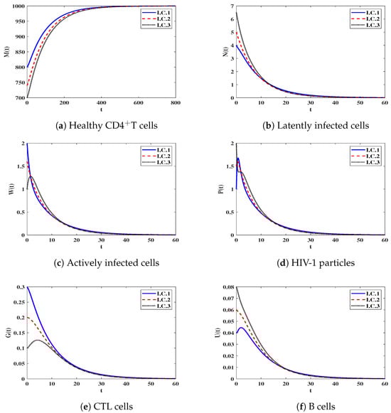
Figure 1. The behavior of solution trajectories of system (12) in the case of ${\Re }_0\le 1$.

Stability of ${\mathbf{Q}}_{\mathbf{1}}$. We let ${\psi }_1=0.001,$ ${\psi }_2=0.0001,$ ${\psi }_3=0.0005,$ $\delta =0.001$ and $\kappa =0.001$. With such a choice, we obtain ${\Re }_0=1.3401>1$. Clearly, the steady state ($Q_1$) exists when ${\Re }_0>1$ with $Q_1=(752.915,6.678,1.653,1.788,0.205,0.059)$. Figure 2 demonstrates that the numerical outcomes are in agreement with the result of Theorem 3, as the solutions of system (12) end up at $Q_1$ when ${\Re }_0>1$ for I.C.1–I.C.3. This case indicates the persistence of HIV-1 infection.

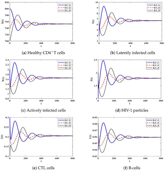
Figure 2. The behavior of solution trajectories of system (12) in case of ${\Re }_0>1$.

3.3.2. Effect of Impaired CTLs and B-Cells

To study the effect of impaired CTLs and B cells, we fix the parameters at ${\psi }_1=0.001,$ ${\psi }_2=0.0001$ and ${\psi }_3=0.0005$ and vary parameters $\delta$ and $\kappa$. We consider the following initial condition:

I.C.4: $\left(M\right(0),N(0),W(0),P(0),G(0\left)\right)=(750,6.8,1.7,1.8,0.1,0.03)$.

We note from Table 2 that increases in $\delta$ and $\kappa$ lead to a reductions in the number of B cells and CTL cells, which, in turn, emphasizes the high number of latently and actively infected cells, as well as HIV-1 particles. Consequently, the number of healthy CD$4^{+}$T cells is decreased. Figure 3 shows that the impairment of immune response has no effect on the stability criteria of the steady states because the ${\Re }_0$ parameter is free of $\delta$ and $\kappa$.

Table 2. Effect of the impairment parameters on the steady states.

$\mathit{\delta }$	$\mathit{\kappa }$	Steady States
$0,$	0	$Q_1=\left(752.967,6.677,1.652,1.787,0.207,0.06\right)$
$0.05,$	$0.06$	$Q_1=\left(751.051,6.728,1.67,1.807,0.147,0.044\right)$
$0.2,$	$0.4$	$Q_1=\left(748.737,6.791,1.691,1.831,0.079,0.018\right)$
$2.4,$	$1.2$	$Q_1=\left(746.589,6.849,1.711,1.854,0.01,0.007\right)$

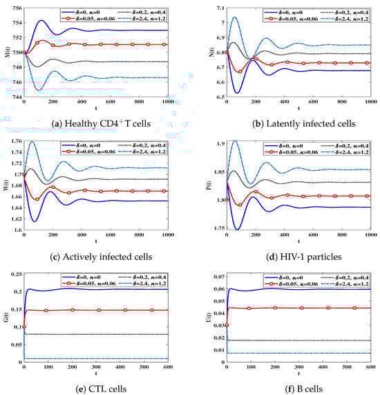
Figure 3. The behavior of solution trajectories of system (12) with different values of $\delta$ and $\kappa$.

3.4. Numerical Simulation for Model (17)

For numerical purposes, we select a specific form of the probability distributed functions ($h_i\left(\upsilon \right),$ $i=1,2,3$) as follows:

$$h_i\left(\upsilon \right)={\delta }_{*}\left(\upsilon -{\upsilon }_i\right),{\upsilon }_i\in \left[0,{\varrho }_i\right],i=1,2,3,$$

where ${\delta }_{*}(.)$ is the Dirac delta function. As ${\varrho }_i\to \infty ,$ we obtain

$${\int }_0^{\infty }{h}_i\left(\upsilon \right)d\upsilon =1,i=1,2,3.$$

Moreover,

$$H_i={\int }_0^{\infty }{\delta }_{*}\left(\upsilon -{\upsilon }_i\right)e^{-k_i\upsilon }d\upsilon =e^{-k_i{\upsilon }_i},i=1,2,3.$$

Hence, we obtain

$$\left\{\begin{array}{cc}{\displaystyle \frac{dM\left(t\right)}{dt}}\hfill & =\mu -{\eta }_{M}M\left(t\right)-{\psi }_{1}M\left(t\right)P\left(t\right)-{\psi }_{2}M\left(t\right)N\left(t\right)-{\psi }_{3}M\left(t\right)W\left(t\right),\hfill \\ {\displaystyle \frac{dN\left(t\right)}{dt}}\hfill & =e^{-k_1{\upsilon }_1}M\left(t-{\upsilon }_1\right)\left({\psi }_{1}P\left(t-{\upsilon }_1\right)+{\psi }_{2}N\left(t-{\upsilon }_1\right)\right.\hfill \\ \hfill & \left.+{\psi }_{3}W\left(t-{\upsilon }_1\right)\right)-(\theta +{\eta }_N)N\left(t\right),\hfill \\ {\displaystyle \frac{dW\left(t\right)}{dt}}\hfill & =\theta e^{-k_2{\upsilon }_2}N\left(t-{\upsilon }_2\right)-{\eta }_{W}W\left(t\right)-\tau G\left(t\right)W\left(t\right),\hfill \\ {\displaystyle \frac{dP\left(t\right)}{dt}}\hfill & =\vartheta e^{-k_3{\upsilon }_3}W\left(t-{\upsilon }_3\right)-{\eta }_{P}P\left(t\right)-\beta U\left(t\right)P\left(t\right),\hfill \\ {\displaystyle \frac{dG\left(t\right)}{dt}}\hfill & =\gamma W\left(t\right)-{\eta }_{G}G\left(t\right)-\delta G\left(t\right)W\left(t\right),\hfill \\ {\displaystyle \frac{dU\left(t\right)}{dt}}\hfill & =\alpha P\left(t\right)-{\eta }_{U}U\left(t\right)-\kappa U\left(t\right)P\left(t\right).\hfill \end{array}\right.$$

(19)

For system (19), the basic reproductive number is given as:

$${\tilde{\Re }}_{0\left(19\right)}=\frac{{\tilde{M}}_0{e}^{-k_1{\upsilon }_1}\left(\theta e^{-k_2{\upsilon }_2}\left({\psi }_1\vartheta e^{-k_3{\upsilon }_3}+{\psi }_3{\eta }_P\right)+{\psi }_2{\eta }_P{\eta }_W\right)}{{\eta }_P{\eta }_W\left(\theta +{\eta }_N\right)}.$$

(20)

Impact of Time Delays on Stability of Steady States

Here, we study the effectiveness of delay values on the dynamics of system (19). To do so, we select ${\psi }_1=0.001,$ ${\psi }_2=0.0001,$ ${\psi }_3=0.0005,$ $\delta =0.001,$ $\kappa =0.001,$ $k_1=0.1,$ $k_2=0.2$ and $k_3=0.3.$ The other parameters are taken from Table 1. Moreover, the delay parameters (${\upsilon }_i,$ $i=1,2,3$) are varied. The dependence of ${\tilde{\Re }}_{0\left(19\right)}$ as presented in Equation (20), on the values of ${\upsilon }_i$ causes a remarkable change in the stability of steady states as long as the ${\upsilon }_i$ parameters are changed. Let us consider following delay values:

DV1: ${\upsilon }_1=0.007$, ${\upsilon }_2=0.006$, ${\upsilon }_3=0.005$.

DV2: ${\upsilon }_1=0.08$, ${\upsilon }_2=0.07$, ${\upsilon }_3=0.09$.

DV3: ${\upsilon }_1=0.2$, ${\upsilon }_2=0.4$, ${\upsilon }_3=0.5$.

DV4: ${\upsilon }_1=0.4$, ${\upsilon }_2=0.6$, ${\upsilon }_3=0.7$.

DV5: ${\upsilon }_1=0.5$, ${\upsilon }_2=0.784$, ${\upsilon }_3=0.8$.

DV6: ${\upsilon }_1=0.9$, ${\upsilon }_2=1.1$, ${\upsilon }_3=1.2$.

• We solve system (19) under the following initial condition:

I.C.5: $\left(M\right(r),N(r),W(r),P(r),G(r),U(r\left)\right)=(850,2,0.5,0.5,0.06,0.02)$, $r\in [-\upsilon ,0],$ $\upsilon =\max \{{\upsilon }_1,{\upsilon }_2,{\upsilon }_3\}$.

In Table 3, we present the values of ${\tilde{\Re }}_{0\left(19\right)}$ for selected values of ${\upsilon }_i,$ $i=1,2,3$. We observe that an increase in the ${\upsilon }_i$ parameters leads to a remarkable decrease in the values of ${\tilde{\Re }}_{0\left(19\right)}$. The numerical solutions are shown in Figure 4. We find that increasing of time delays increases the concentration of healthy CD$4^{+}$T cells and decreases the concentration of other compartments.

Table 3. The variation of ${\tilde{\Re }}_{0\left(19\right)}$ with respect to ${\varrho }_i$.

Delay Parameters (${\mathit{\upsilon }}_1,{\mathit{\upsilon }}_2,{\mathit{\upsilon }}_3$)	Steady States	${\tilde{\mathit{\Re }}}_{0\left(19\right)}$
$0.007,0.006,0.005$	${\tilde{Q}}_{1\left(19\right)}=(754.718,6.625,1.638,1.769,0.203,0.059)$	$1.337$
$0.08,0.07,0.09$	${\tilde{Q}}_{1\left(19\right)}=(777.899,5.955,1.455,1.532,0.181,0.051)$	$1.296$
$0.2,0.4,0.5$	${\tilde{Q}}_{1\left(19\right)}=(879.981,3.18,0.73,0.681,0.091,0.023)$	$1.141$
$0.4,0.6,0.7$	${\tilde{Q}}_{1\left(19\right)}=(950.874,1.276,0.282,0.248,0.035,0.008)$	$1.053$
$0.5,0.784,0.8$	${\tilde{Q}}_{0\left(19\right)}=(1000,0,0,0,0,0)$	1
$0.9,1.1,1.2$	${\tilde{Q}}_{0\left(19\right)}=(1000,0,0,0,0,0)$	$0.869$

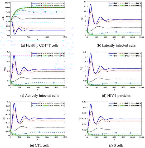
Figure 4. The influence of time delay parameters on the behavior of solution trajectories of system (19).

3.5. Sensitivity Analysis

3.5.1. Sensitivity Analysis for Model (12)

The main goal of a sensitivity analysis is to identify the variable that carries the greatest risk. We apply partial derivatives to calculate the sensitivity index when variables vary based on parameters. The normalized forward sensitivity index of ${\Re }_0$ is expressed using the following parameter:

$${\Xi }_{\aleph }=\frac{\aleph }{{\Re }_0}\frac{\partial {\Re }_0}{\partial \aleph },$$

(21)

where ℵ is a given parameter. We use Equation (21) to determine the sensitivity indices for each parameter given in ${\Re }_0$ based on the values listed in Table 1 with ${\psi }_1=0.001$, ${\psi }_2=0.0001$ and ${\psi }_3=0.0005$. Table 4 and Figure 5 show the value of the sensitivity index of ${\Re }_0$. It is evident that $\mu$, ${\psi }_1$, ${\psi }_2$, ${\psi }_3$, $\vartheta$ and $\theta$ have positive index values. Consequently, there is a correlation between increased in the values of these parameters and the endemicity of the HIV-1 disease. The other indices are negative, which means that when the values of ${\eta }_M$, ${\eta }_P$, ${\eta }_N$ and ${\eta }_W$ increase, the value of ${\Re }_0$ decreases. Obviously, the most crucial parameters in terms of sensitivity are $\mu$, ${\psi }_1$ and $\vartheta$, while ${\psi }_2$, ${\psi }_3$ and $\theta$ are the least crucial. The parameters of CTL and B-cell responsiveness, $\gamma$ and $\alpha$, respectively, have no effect on ${\Re }_0$.

Table 4. Sensitivity index of ${\Re }_0$ for model (12).

Parameter ℵ	Value of ${\mathsf{\Xi }}_{\mathsf{\aleph }}$	Parameter ℵ	Value of ${\mathsf{\Xi }}_{\mathsf{\aleph }}$
$\mu$	1	$\vartheta$	$0.546$
${\eta }_M$	$-1$	$\theta$	$0.258$
${\psi }_1$	$0.546$	${\eta }_P$	$-0.546$
${\psi }_2$	$0.202$	${\eta }_N$	$-0.459$
${\psi }_3$	$0.252$	${\eta }_W$	$-0.798$

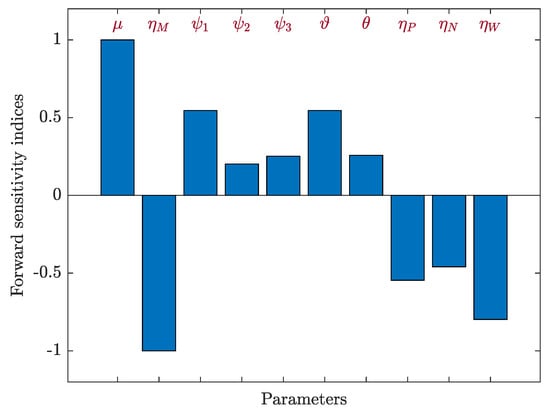
Figure 5. Forward sensitivity analysis of the ${\Re }_0$ parameters of system (12).

3.5.2. Sensitivity Analysis for Model (19)

We used Equation (21) with respect to ${\tilde{\Re }}_{0\left(19\right)}$ to determine the sensitivity indices for each parameter in ${\tilde{\Re }}_{0\left(19\right)}$ based on the parameter values in Table 1 and the following values: ${\psi }_1=0.001$, ${\psi }_2=0.0001$, ${\psi }_3=0.0005$, $k_1=0.1$, $k_2=0.2$, $k_3=0.3$, ${\upsilon }_1=0.2$, ${\upsilon }_2=0.4$ and ${\upsilon }_3=0.5$. Table 5 and Figure 6 show the value of the sensitivity index of ${\tilde{\Re }}_{0\left(19\right)}$. Since $\mu$, ${\psi }_1$, ${\psi }_2$, ${\psi }_3$, $\vartheta$ and $\theta$ have positive indices, an increase in these values results in an increase in the endemicity of the HIV-1 disease. Increasing negative index values, i.e., ${\eta }_P$, ${\eta }_N$, ${\eta }_W$, $k_1$, $k_2$, $k_3$, ${\upsilon }_1$, ${\upsilon }_2$ and ${\upsilon }_3$, results in a decrease in the value of ${\tilde{\Re }}_{0\left(19\right)}$. We can see that $\mu$, ${\psi }_1$ and $\vartheta$ are the most effective parameters, and ${\psi }_2$, ${\psi }_3$ and $\theta$ are the least effective.

Table 5. Sensitivity index of ${\tilde{\Re }}_{0\left(19\right)}$ of model (19).

Parameter ℵ	Value of ${\mathsf{\Xi }}_{\mathsf{\aleph }}$	Parameter ℵ	Value of ${\mathsf{\Xi }}_{\mathsf{\aleph }}$
$\mu$	1	${\eta }_N$	$-0.459$
${\eta }_M$	$-1$	${\eta }_W$	$-0.768$
${\psi }_1$	$0.5$	$k_1$	$-0.02$
${\psi }_2$	$0.232$	$k_2$	$-0.061$
${\psi }_3$	$0.268$	$k_3$	$-0.075$
$\vartheta$	$0.5$	${\upsilon }_1$	$-0.02$
$\theta$	$0.227$	${\upsilon }_2$	$-0.061$
${\eta }_P$	$-0.5$	${\upsilon }_3$	$-0.075$

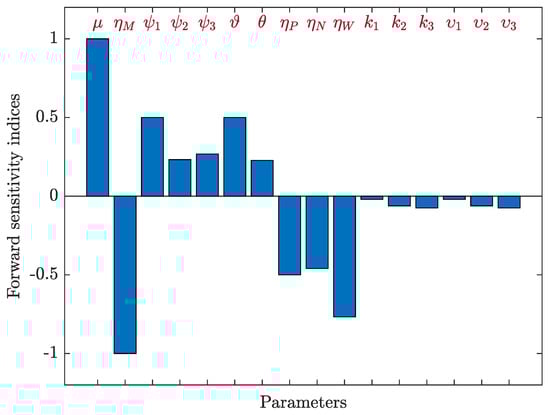
Figure 6. Forward sensitivity analysis of the ${\tilde{\Re }}_{0\left(19\right)}$ parameters of system (19).

4. Conclusions and Discussion

In this study, we developed two models to get insights into the effect of impaired CTL and B-cell functions on HIV-1 dynamics. These models consist of six compartments: healthy CD$4^{+}$T cells, latently infected cells, actively infected cells, free HIV-1 particles, CTLs and B cells. To be more realistic, we assumed that the healthy CD$4^{+}$T cells became infected by coming into contact with free HIV-1 particles, latently infected cells and actively infected cells. In the second model, we included three distributed time delays to improve precision. We showed that the solutions of the models are non-negative and bounded. We found that the models have two steady states: an infection-free steady state ($Q_0$ or ${\tilde{Q}}_0$) and an infected steady state ($Q_1$ or ${\tilde{Q}}_1$). We calculated the basic reproductive numbers (${\Re }_0$ or ${\tilde{\Re }}_0$) that control the existence of the two steady states and their global stability. The ${\Re }_0$ number (or ${\tilde{\Re }}_0$) is based on three terms: the first is due to the VT mechanism, the second is the effect of the latent CT mechanism and the third term is the influence of the active CT mechanism. For each model, we built up Lyapunov functions and employed L.I.P to examine the global asymptotic stability of the two steady states. We showed that if ${\Re }_0\le 1$ (or ${\tilde{\Re }}_0\le 1$), then $Q_0$ (or ${\tilde{Q}}_0$) is G.A.S, with the HIV-1 infection going extinct eventually. From a control point of view, ${\Re }_0\le 1$ (or ${\tilde{\Re }}_0\le 1$) can be achieved by designing a different class of antiviral drug therapies. On the other hand, if ${\Re }_0>1$ (or ${\tilde{\Re }}_0>1$), then $Q_0$ (or ${\tilde{Q}}_0$) is unstable, and $Q_1$ (or ${\tilde{Q}}_1$) is G.A.S; then, the HIV-1 infection is chronic. We executed some numerical simulations to emphasize our theoretical outcomes. We determined that the numerical results are in agreement with the theoretical results.

We discussed the effect of B-cell and CTL impairment, time delay and the latent CT mechanism on the dynamics of HIV-1. We showed that weak adaptive immunity significantly affects the progression of the disease. Furthermore, enlarging the delay period can decrease the basic reproductive number (${\tilde{\Re }}_0$) and inhibit HIV-1 replication. This provides some insights for the development of a new class of HIV-1 treatment to prolong the delay period. Furthermore, we found that ignoring the latent CT mechanism in the HIV-1 dynamics model causes an underestimation of the basic reproductive number; thus, the designed drug doses may be inaccurate or insufficient to clear the virus from the body. This shows the importance of including the latent CT mechanism in our proposed models. In addition, we conducted a sensitivity analysis to show how ${\Re }_0$ (or ${\tilde{\Re }}_0$) can be affected by the values of all parameters of the proposed models given certain data.

The main limitation of the present work is that we did not use real data to estimate the values of the model’s parameters. In [57], virus concentration measurements were obtained from the peripheral blood of ten patients collected at three labs. The authors used the following 3D HIV-1 model:

$$\begin{array}{cc}\hfill {\displaystyle \frac{dM\left(t\right)}{dt}}& =\mu -{\eta }_{M}M\left(t\right)-\psi M\left(t\right)P\left(t\right),\hfill \end{array}$$

(22)

$$\begin{array}{cc}\hfill {\displaystyle \frac{dW\left(t\right)}{dt}}& =\psi M\left(t\right)P\left(t\right)-{\eta }_{W}W\left(t\right),\hfill \end{array}$$

(23)

$$\begin{array}{cc}\hfill {\displaystyle \frac{dP\left(t\right)}{dt}}& =\vartheta W\left(t\right)-{\eta }_{P}P\left(t\right),\hfill \end{array}$$

(24)

and estimated only four parameters: ${\eta }_M$, $\psi$, ${\eta }_W$ and $\vartheta$. In [58], the model (22)–(24) was fitted to a clinical dataset to estimate the dynamic parameters in six HIV-1-infected individuals administered antiretroviral treatment. The ${\eta }_M$, $\psi$, ${\eta }_W$ and N parameters were estimated, where $N=\vartheta /{\eta }_W$ is the number of new virions produced by each infected cell during its lifetime. We note that the number of parameters to be estimated in our model (12) is 18. A minimum number of measurements is required to identify the model’s parameters (see e.g., [58,59]). When only the virus can be measured, a large number of measurements is needed to estimate the parameters of our model, which is a difficult task. Frequently, only viral load data are available, and in this case, not all parameters can be identified independently [57,58]. When identifying HIV-1 models, there are typically few data available [60]. A patient receiving effective therapy often has his or her viral load checked every three to four months, which is too infrequent to capture the dynamic characteristics [60]. Ciupe et al. [61] used the data presented in [57] to estimate some of the model’s parameters. We obtained more data than reported in [57]; however, these data may not be sufficient to uniquely determine the 18 parameters of our model. Thus, the theoretical results obtained in this paper need to be tested against empirical findings when real data become available.

Future Works

Model (17) can be improved by:

• Modify the model by adding the diffusion of all compartments as:

  $$\begin{array}{cc}\hfill \frac{\partial M(t,\phi )}{\partial t}-{\varsigma }_M\Delta M\left(t,\phi \right)& =\mu -{\eta }_{M}M\left(t,\phi \right)-{\psi }_{1}M\left(t,\phi \right)P\left(t,\phi \right)-{\psi }_{2}M\left(t,\phi \right)N\left(t,\phi \right),\hfill \\ \hfill & -{\psi }_{3}M\left(t,\phi \right)W\left(t,\phi \right)\hfill \\ \hfill \frac{\partial N\left(t,\phi \right)}{\partial t}-{\varsigma }_N\Delta N\left(t,\phi \right)& ={\int }_0^{{\varrho }_1}{h}_1\left(\upsilon \right)e^{-k_1\upsilon }M\left(t-\upsilon ,\phi \right)\left({\psi }_{1}P\left(t-\upsilon ,\phi \right)+{\psi }_{2}N\left(t-\upsilon ,\phi \right)\right.\hfill \\ \hfill & \left.+{\psi }_{3}W\left(t-\upsilon ,\phi \right)\right)d\upsilon -(\theta +{\eta }_N)N\left(t,\phi \right),\hfill \\ \hfill \frac{\partial W\left(t,\phi \right)}{\partial t}-{\varsigma }_W\Delta W\left(t,\phi \right)& =\theta {\int }_0^{{\varrho }_2}{h}_2\left(\upsilon \right)e^{-k_2\upsilon }N\left(t-\upsilon ,\phi \right)d\upsilon -{\eta }_{W}W\left(t,\phi \right)-\tau G(t,\phi )W(t,\phi ),\hfill \\ \hfill \frac{\partial P\left(t,\phi \right)}{\partial t}-{\varsigma }_P\Delta P\left(t,\phi \right)& =\vartheta {\int }_0^{{\varrho }_3}{h}_3\left(\upsilon \right)e^{-k_3\upsilon }W\left(t-\upsilon ,\phi \right)d\upsilon -{\eta }_{P}P\left(t,\phi \right)-\beta U(t,\phi )P(t,\phi ),\hfill \\ \hfill \frac{\partial G\left(t,\phi \right)}{\partial t}-{\varsigma }_G\Delta G\left(t,\phi \right)& =\gamma W(t,\phi )-{\eta }_{G}G(t,\phi )-\delta G(t,\phi )W(t,\phi ),\hfill \\ \hfill \frac{\partial U\left(t,\phi \right)}{\partial t}-{\varsigma }_U\Delta U\left(t,\phi \right)& =\alpha P(t,\phi )-{\eta }_{U}U(t,\phi )-\kappa U(t,\phi )P(t,\phi ),\hfill \end{array}$$

  where $\phi$ is the position, $\Delta =\frac{{\partial }^2}{\partial {\phi }^2}$ and ${\varsigma }_u$ is the diffusion coefficient of compartment u.
• Using real data to estimate the model’s parameters;
• Considering the age structure in the infected cells;
• Considering viral mutations.

These points will be left for future consideration.

References

- Wodarz, D.; Levy, D.N. Human immunodeficiency virus evolution towards reduced replicative fitness in vivo and the development of AIDS. Proc. R. Soc. Biol. Sci. 2007, 274, 2481–2491. [Google Scholar] [CrossRef]
- Available online: https://www.who.int/data/gho/data/themes/hiv-aids (accessed on 1 September 2023).
- Nowak, M.A.; Bangham, C.R.M. Population dynamics of immune responses to persistent viruses. Science 1996, 272, 74–79. [Google Scholar] [CrossRef]
- Nowak, M.A.; May, R.M. Virus Dynamics; Oxford University Press: New York, NY, USA, 2000. [Google Scholar]
- Lv, C.; Huang, L.; Yuan, Z. Global stability for an HIV-1 infection model with Beddington-DeAngelis incidence rate and CTL immune response. Commun. Nonlinear Sci. Numer. Simul. 2014, 19, 121–127. [Google Scholar] [CrossRef]
- Jiang, C.; Kong, H.; Zhang, G.; Wang, K. Global properties of a virus dynamics model with self-proliferation of CTLs. Math. Appl. Sci. Eng. 2021, 2, 123–133. [Google Scholar] [CrossRef]
- Ren, J.; Xu, R.; Li, L. Global stability of an HIV infection model with saturated CTL immune response and intracellular delay. Math. Biosci. Eng. 2020, 18, 57–68. [Google Scholar] [CrossRef] [PubMed]
- Wang, A.P.; Li, M.Y. Viral dynamics of HIV-1 with CTL immune response. Discret. Contin. Dyn. Syst. Ser. B 2021, 26, 2257–2272. [Google Scholar] [CrossRef]
- Yang, Y.; Xu, R. Mathematical analysis of a delayed HIV infection model with saturated CTL immune response and immune impairment. J. Appl. Math. Comput. 2022, 68, 2365–2380. [Google Scholar] [CrossRef]
- Chen, C.; Zhou, Y. Dynamic analysis of HIV model with a general incidence, CTLs immune response and intracellular delays. Math. Comput. Simul. 2023, 212, 159–181. [Google Scholar] [CrossRef]
- Wodarz, D.; May, R.M.; Nowak, M.A. The role of antigen-independent persistence of memory cytotoxic T lymphocytes. Int. Immunol. 2000, 12, 467–477. [Google Scholar] [CrossRef]
- Elaiw, A.M.; AlShamrani, N.H. Global stability of humoral immunity virus dynamics models with nonlinear infection rate and removal. Nonlinear Anal. Real World Appl. 2015, 26, 161–190. [Google Scholar] [CrossRef]
- Wang, S.; Zou, D. Global stability of in host viral models with humoral immunity and intracellular delays. Appl. Math. Model. 2012, 36, 1313–1322. [Google Scholar] [CrossRef]
- Tang, S.; Teng, Z.; Miao, H. Global dynamics of a reaction–diffusion virus infection model with humoral immunity and nonlinear incidence. Comput. Math. Appl. 2019, 78, 786–806. [Google Scholar] [CrossRef]
- Zheng, T.; Luo, Y.; Teng, Z. Spatial dynamics of a viral infection model with immune response and nonlinear incidence. Z. Für Angew. Math. Und Phys. 2023, 74, 124. [Google Scholar] [CrossRef] [PubMed]
- Kajiwara, T.; Sasaki, T.; Otani, Y. Global stability for an age-structured multistrain virus dynamics model with humoral immunity. J. Appl. Math. Comput. 2020, 62, 239–279. [Google Scholar] [CrossRef]
- Dhar, M.; Samaddar, S.; Bhattacharya, P. Modeling the effect of non-cytolytic immune response on viral infection dynamics in the presence of humoral immunity. Nonlinear Dyn. 2019, 98, 637–655. [Google Scholar] [CrossRef]
- Murase, A.; Sasaki, T.; Kajiwara, T. Stability analysis of pathogen-immune interaction dynamics. J. Math. Biol. 2005, 51, 247–267. [Google Scholar] [CrossRef]
- Wodarz, D. Hepatitis C virus dynamics and pathology: The role of CTL and antibody responses. J. Gen. Virol. 2003, 84, 1743–1750. [Google Scholar] [CrossRef] [PubMed]
- Wang, J.; Pang, J.; Kuniya, T.; Enatsu, Y. Global threshold dynamics in a five-dimensional virus model with cell-mediated, humoral immune responses and distributed delays. Appl. Math. Comput. 2014, 241, 298–316. [Google Scholar] [CrossRef]
- Yan, Y.; Wang, W. Global stability of a five-dimensional model with immune responses and delay. Discret. Contin. Dyn. Syst. Ser. B 2012, 17, 401–416. [Google Scholar] [CrossRef]
- Dubey, P.; Dubey, U.S.; Dubey, B. Modeling the role of acquired immune response and antiretroviral therapy in the dynamics of HIV infection. Math. Comput. Simul. 2018, 144, 120–137. [Google Scholar] [CrossRef]
- Mondal, J.; Samui, P.; Chatterjee, A.N. Dynamical demeanour of SARS-CoV-2 virus undergoing immune response mechanism in COVID-19 pandemic. Eur. Phys. J. Spec. Top. 2022, 231, 3357–3370. [Google Scholar] [CrossRef]
- Sigal, A.; Kim, J.T.; Balazs, A.B.; Dekel, E.; Mayo, A.; Milo, R.; Baltimore, D. Cell-to-cell spread of HIV permits ongoing replication despite antiretroviral therapy. Nature 2011, 477, 95–98. [Google Scholar] [CrossRef]
- Martin, N.; Sattentau, Q. Cell-to-cell HIV-1 spread and its implications for immune evasion. Curr. Opin. HIV Aids 2009, 4, 143–149. [Google Scholar] [CrossRef] [PubMed]
- Dhar, M.; Samaddar, S.; Bhattacharya, P. Modeling the cell-to-cell transmission dynamics of viral infection under the exposure of non-cytolytic cure. J. Appl. Math. Comput. 2021, 65, 885–911. [Google Scholar] [CrossRef]
- Lin, J.; Xu, R.; Tian, X. Threshold dynamics of an HIV-1 virus model with both virus-to-cell and cell-to-cell transmissions, intracellular delay, and humoral immunity. Appl. Math. Comput. 2017, 315, 516–530. [Google Scholar] [CrossRef]
- Luo, Y.; Zhang, L.; Zheng, T.; Teng, Z. Analysis of a diffusive virus infection model with humoral immunity, cell-to-cell transmission and nonlinear incidence. Phys. A 2019, 535, 122415. [Google Scholar] [CrossRef]
- Wang, J.; Guo, M.; Liu, X.; Zhao, Z. Threshold dynamics of HIV-1 virus model with cell-to-cell transmission, cell-mediated immune responses and distributed delay. Appl. Math. Comput. 2016, 291, 149–161. [Google Scholar] [CrossRef]
- Cervantes-Perez, A.G.; Avila-Vales, E. Dynamical analysis of multipathways and multidelays of general virus dynamics model. Int. J. Bifurc. Chaos 2019, 29, 1950031. [Google Scholar] [CrossRef]
- Lin, J.; Xu, R.; Tian, X. Threshold dynamics of an HIV-1 model with both viral and cellular infections, cell-mediated and humoral immune responses. Math. Biosci. Eng. 2018, 16, 292–319. [Google Scholar] [CrossRef]
- Hattaf, K.; Yousfi, N. Modeling the adaptive immunity and both modes of transmission in HIV infection. Computation 2018, 6, 37. [Google Scholar] [CrossRef]
- Elaiw, A.M.; AlShamrani, N.H. Global stability of a delayed adaptive immunity viral infection with two routes of infection and multi-stages of infected cells. Commun. Nonlinear Sci. Numer. Simul. 2020, 86, 105259. [Google Scholar] [CrossRef]
- Agosto, L.; Herring, M.; Mothes, W.; Henderson, A. HIV-1-infected CD4+ T cells facilitate latent infection of resting CD4+ T cells through cell-cell contact. Cell 2018, 24, 2088–2100. [Google Scholar] [CrossRef] [PubMed]
- Wang, W.; Wang, X.; Guo, K.; Ma, W. Global analysis of a diffusive viral model with cell-to-cell infection and incubation period. Math. Methods Appl. Sci. 2020, 43, 5963–5978. [Google Scholar] [CrossRef]
- Elaiw, A.M.; AlShamrani, N.H.; Hobiny, A.D.; Abbas, I.A. Global stability of an adaptive immunity HIV dynamics model with silent and active cell-to-cell transmissions. AIP Adv. 2020, 10, 085216. [Google Scholar] [CrossRef]
- Lydyard, P.; Whelan, A.; Fanger, M. BIOS Instant Notes in Immunology; Taylor & Francis e-Library: New York, NY, USA, 2005. [Google Scholar]
- Regoes, R.; Wodarz, D.; Nowak, M.A. Virus dynamics: The effect to target cell limitation and immune responses on virus evolution. J. Theor. Biol. 1998, 191, 451–462. [Google Scholar] [CrossRef] [PubMed]
- Hu, Z.; Zhang, J.; Wang, H.; Ma, W.; Liao, F. Dynamics analysis of a delayed viral infection model with logistic growth and immune impairment. Appl. Math. Model. 2014, 38, 524–534. [Google Scholar] [CrossRef]
- Krishnapriya, P.; Pitchaimani, M. Modeling and bifurcation analysis of a viral infection with time delay and immune impairment. Jpn. J. Ind. Appl. Math. 2017, 34, 99–139. [Google Scholar] [CrossRef]
- Wang, S.; Song, X.; Ge, Z. Dynamics analysis of a delayed viral infection model with immune impairment. Appl. Math. Model. 2011, 35, 4877–4885. [Google Scholar] [CrossRef]
- Krishnapriya, P.; Pitchaimani, M. Analysis of time delay in viral infection model with immune impairment. J. Appl. Math. Comput. 2017, 55, 421–453. [Google Scholar] [CrossRef]
- Wang, Z.P.; Liu, X.N. A chronic viral infection model with immune impairment. J. Theor. Biol. 2007, 249, 532–542. [Google Scholar] [CrossRef]
- Alofi, B.S.; Azoz, S.A. Stability of general pathogen dynamic models with two types of infectious transmission with immune impairment. AIMS Math. 2020, 6, 114–140. [Google Scholar] [CrossRef]
- Elaiw, A.M.; Raezah, A.; Alofi, B.S. Dynamics of delayed pathogen infection models with pathogenic and cellular infections and immune impairment. AIP Adv. 2018, 8, 025323. [Google Scholar] [CrossRef]
- Zhang, L.; Xu, R. Dynamics analysis of an HIV infection modelwith latent reservoir, delayed CTL immune response and immune impairment. Nonlinear Anal. Model. Control. 2023, 28, 1–19. [Google Scholar] [CrossRef]
- Miao, H.; Abdurahman, X.; Teng, Z.; Zhang, L. Dynamical analysis of a delayed reaction-diffusion virus infection model with logistic growth and humoral immune impairment. Chaos Solitons Fractals 2018, 110, 280–291. [Google Scholar] [CrossRef]
- Elaiw, A.M.; Alshehaiween, S.F.; Hobiny, A.D. Global properties of HIV dynamics models including impairment of B-cell functions. J. Biol. Syst. 2020, 28, 1–25. [Google Scholar] [CrossRef]
- Elaiw, A.M.; Alshehaiween, S.F. Global stability of delay-distributed viral infection model with two modes of viral transmission and B-cell impairment. Math. Methods Appl. Sci. 2020, 43, 6677–6701. [Google Scholar] [CrossRef]
- Elaiw, A.M.; Alshehaiween, S.F.; Hobiny, A.D. Impact of B-cell impairment on virus dynamics with time delay and two modes of transmission. Chaos Solitons Fractals 2020, 130, 109455. [Google Scholar] [CrossRef]
- Wang, X.; Rong, L. HIV low viral load persistence under treatment: Insights from a model of cell-to-cell viral transmission. Appl. Math. Lett. 2019, 94, 44–51. [Google Scholar] [CrossRef]
- Hale, J.K.; Lunel, S.M.V. Introduction to Functional Differential Equations; Springer: New York, NY, USA, 1993. [Google Scholar]
- Kuang, Y. Delay Differential Equations with Applications in Population Dynamics; Academic Press: San Diego, CA, USA, 1993. [Google Scholar]
- Sahani, S.K.; Yashi. Effects of eclipse phase and delay on the dynamics of HIV infection. J. Biol. Syst. 2018, 26, 421–454. [Google Scholar] [CrossRef]
- Allali, K.; Danane, J.; Kuang, Y. Global analysis for an HIV infection model with CTL immune response and infected cells in eclipse phase. Appl. Sci. 2017, 7, 861. [Google Scholar] [CrossRef]
- Sun, C.; Li, L.; Jia, J. Hopf bifurcation of an HIV-1 virus model with two delays and logistic growth. Math. Model. Nat. Phenom. 2020, 15, 16. [Google Scholar] [CrossRef]
- Stafford, M.A.; Corey, L.; Cao, Y.; Daar, E.S.; Ho, D.D.; Perelson, A.S. Modeling plasma virus concentration during primary HIV infection. J. Theor. Biol. 2000, 203, 285–301. [Google Scholar] [CrossRef] [PubMed]
- Wu, H.; Zhu, H.; Miao, H.; Perelson, A.S. Parameter identifiability and estimation of HIV/AIDS dynamic models. Bull. Math. Biol. 2008, 70, 785–799. [Google Scholar] [CrossRef] [PubMed]
- Miao, H.; Xia, X.; Perelson, A.S.; Wu, H. On identifiability of nonlinear ODE models and applications in viral dynamics. SIAM Rev. 2011, 53, 3–39. [Google Scholar] [CrossRef] [PubMed]
- Luo, R.; Piovoso, M.J.; Martinez-Picado, J.; Zurakowski, R. HIV model parameter estimates from interruption trial data including drug efficacy and reservoir dynamics. PLoS ONE 2012, 7, e40198. [Google Scholar] [CrossRef] [PubMed]
- Ciupe, M.S.; Bivort, B.L.; Bortz, D.M.; Nelson, P.W. Estimating kinetic parameters from HIV primary infection data through the eyes of three different mathematical models. Math. Biosci. 2006, 200, 1–27. [Google Scholar] [CrossRef]
- Van den Driessche, P.; Watmough, J. Reproduction numbers and sub-threshold endemic equilibria for compartmental models of disease transmission. Math. Biosci. 2002, 180, 29–48. [Google Scholar] [CrossRef]
Disclaimer/Publisher’s Note: The statements, opinions and data contained in all publications are solely those of the individual author(s) and contributor(s) and not of MDPI and/or the editor(s). MDPI and/or the editor(s) disclaim responsibility for any injury to people or property resulting from any ideas, methods, instructions or products referred to in the content. |
© 2023 by the authors. Licensee MDPI, Basel, Switzerland. This article is an open access article distributed under the terms and conditions of the Creative Commons Attribution (CC BY) license (https://creativecommons.org/licenses/by/4.0/).