Polynomial-Based Non-Uniform Ternary Interpolation Surface Subdivision on Quadrilateral Mesh

Abstract

For non-uniform control polygons, a parameterized four-point interpolation curve ternary subdivision scheme is proposed, and its convergence and continuity are demonstrated. Following curve subdivision, a non-uniform interpolation surface ternary subdivision on regular quadrilateral meshes is proposed by applying the tensor product method. Analyses were conducted on the updating rules of parameters, proving that the limit surface is continuous. In this paper, we present a novel interpolation subdivision method to generate new virtual edge points and new face points of the extraordinary points of quadrilateral mesh. We also provide numerical examples to assess the validity of various interpolation methods.

1. Introduction

With the rapid development of information technology, digital multimedia information has penetrated into every corner of contemporary society, such as comics, point cloud reconstruction, etc. Classical geometric modeling methods, such as Bezier surface, B-spline surface, and NURBS surface models, have struggled to satisfy the needs of people. As a discrete modeling design method for curves and surfaces, the subdivision method is an organic combination of the polygonal mesh representation method and the parameter representation method and has become a research hot spot in the field of computer graphics, with its advantage of not being limited by topology. In 1978, Catmull and Clark [1] proposed a subdivision method to extend B-spline surfaces to arbitrary topological meshes. In the 1980s, Doo and Sabin [2] analyzed the continuity of B-spline surface subdivision on irregular meshes, marking the introduction of the surface subdivision technique in the field of surface modeling design.

Surface subdivision is based on an initial mesh; by adding new vertices and adjusting old vertices, a gradually denser mesh sequence is obtained. In this process, if the old vertex position is not modified, it is called interpolation subdivision (Kobbelt [3], Li [4,5]); otherwise, it is called approximation subdivision (Catmull-Clark, Loop [6], $\sqrt{2}$ [7], $\sqrt{3}$ [8], Ni [9]). Approximation subdivision is associated with higher continuity and smoothness than interpolation subdivision; however, it is easy to lose the geometric characteristics of the mesh or obtain a large fitting effect error.

If the subdivision rules do not change throughout the process, the subdivision is known as stationary subdivision (Catmull-Clark, Doo-Sabin, Chaikin [10], Dyn [11], Butterfly [12]); otherwise, it is known as non-stationary subdivision (NURSS [13], NURSSes [14], NULISS [15], NUISS [16]). In engineering applications, the non-stationary subdivision method is preferred relative to the stationary subdivision method for detail maintenance and is more practicable, although it is not as efficient as the static subdivision method in computing. If the control mesh is relatively uniform (the difference between side lengths is small) and has many control vertices, the designers tend is to use stationary subdivision.

In computer graphics and computer-aided design, geometric data parameterization has become an important processing tool that has been widely utilized in data fitting, grid operation, computer animation, and other fields [17,18,19,20,21]. In curve interpolation, the parameter values (also called knots) of the vertices of a given control point have a considerable influence on the generated curve because the knots can be regarded as the time when a particle passes through the control points in sequence along the curve. If uniform parameterization is adopted, the time for the particle to pass through each piecewise curve is the identical. In a longer piecewise curve, particles move at a higher velocity; if the next segment curve is shorter, the particle speed drops sharply, which causes the curve to self-intersect. In 1999, Daubechies [17] introduced non-uniform parameterization and proposed a non-uniform parameterized interpolation subdivision curve. In 2013, Beccari [15] applied the parameterization method to a surface, proposed a non-uniform parameterized surface subdivision method on regular quadrilateral meshes, and analyzed the continuity of the limit surface. Unfortunately, the author did not account for the surface subdivision of quadrilateral meshes with extraordinary points. In 2018, based on the relationship between B-spline curve and four-point interpolation subdivision schemes, Li [16] presented a non-uniform parameterized subdivision method for surface meshes with extraordinary points; however, the specific mask expression not provided in the paper.

In Beccari and Li’s papers, the limit surfaces with C¹ continuity were generated on the basis of four-point binary curve subdivision. In the process of surface generation, owing to the large number of vertices, edges, and faces involved, computer processing is more complicated, with a longer time required to generate the limit surface. Four-point ternary curve subdivision, as mentioned in [22,23,24,25], has a faster convergence speed, and the limit curve has better continuity. In 2018, using a different geometric method, Omar et al. [26] obtained subdivision schemes on quadrilateral mesh based on 2D Lagrange interpolation polynomials.

The main idea of this paper is to calculate the mask of a subdivision scheme by using the chord length parameter and Lagrangian basis function (polynomial-based, Similar to [27]). The four-point ternary curve subdivision scheme is constructed according to the mask. Surface subdivision is a natural generalization of curve subdivision on quadrilateral mesh.

In this thesis, the following aspects are considered:

(1).

A polynomial-based non-uniform four-point ternary interpolation curve subdivision method is proposed, and we prove that the limit curve of this scheme C¹ continuous;

(2).

For regular quadrilateral meshes, using four-point ternary curve subdivision and tensor product, we construct a ternary interpolation surface subdivision scheme on non-uniform regular quadrilateral meshes and prove that the limit surface is C¹ is continuous at any point;

(3).

By constructing virtual points for meshes with extraordinary points, a ternary interpolation method of new edge points and new face points of the extraordinary point is proposed. Due to the lack of an effective method, the convergence and G¹ continuity of the limit surface are illustrated by analyzing the change trend of the angles between normal vectors at the extraordinary points.

The remainder of this paper is organized as follows. In Section 2, we review the content of curve parameterization, define a non-uniform four-point ternary curve subdivision (NUFTCS) by parameterization, and prove the convergence of the subdivision scheme and the continuity of the limit curve. In Section 3, using tensor product combined with NUFTCS, a non-uniform local ternary interpolation surface subdivision (NULTISS) method is proposed under a regular quadrilateral mesh, and the continuity of the limit surface is analyzed. For extraordinary points, the rules of generating new edge points and new face points, as well as the empirical analysis, are presented in Section 4. In Section 5, we present some numerical examples of curve subdivision and surface subdivision, confirming the effectiveness of our proposed method. In Section 6, we summarize the study results and the introduce concepts for follow-up works.

2. Non-Uniform Four-Point Ternary Curve Subdivision (NUFTCS)

2.1. Parameterization of the Data Points

With the data points of the initial control polygon denoted by $\left\{P_i\left(x_i,y_i\right),i=0,1,2,\cdots \right\}$, we can construct a function ($y=f\left(x\right)$) by Lagrange polynomial interpolation to satisfy $f\left(x_i \right)=y_i,i=0,1,2,\cdots$. Parameterization of data points is the process of assigning parameter values to a set of ordered data points, as shown in Figure 1 (left). The parameterization of data points should reflect the nature of the interpolated data or the desired nature of the designer to the greatest extent possible. Commonly used data point parameterization methods include uniform parameterization, centripetal parameterization, and chordal parameterization, e.g.,

$$\left\{\begin{array}{c}{t}_0=0,\\ t_i=t_{i-1}+d_i, i=0,1,2,\cdots ,n, \end{array}\right.$$

(1)

where $d_{i-1}= \Vert P_i-P_{i-1}\Vert {}^{\alpha }$; $\alpha =0$ results in uniform parameterization, $\alpha =1$ results in chordal parameterization, and $\alpha =\frac{1}{2}$ corresponds to centripetal parameterization. Chordal parameterization is generally considered to be the most effective method of curve parameterization. In this study, it is used to construct the mask of curve subdivision.

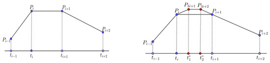
Figure 1. Parameterization of the data points. Left: $t_{i+k}$ is the parameter of the initial control point, $P_{i+k}$, $k=-1,0,1,2$. Right: $t_1^{*},t_2^{*}$ are the parameters of the new control points, $P_{3i+1}$ and $P_{3i+2}$, respectively.

2.2. Non-Uniform Four-Point Ternary Curve Subdivision (NUFTCS)

As shown in Figure 1 (right), let $P=\left\{P_i\right\}$,$i\in \mathbb{Z}$ be a set of data points and $T=\left\{t_i \right\},i\in \mathbb{Z}$ be the associated parameter set; then, $d_i=t_{i+1}-t_i= \Vert P_{i+1}-P_i\Vert ,i\in \mathbb{Z}$, introduces the notation ${\alpha }_i=\left[d_{i-1},d_i,d_{i+1}\right]$ (called the mask parameter).

Using $t_{i-1},t_i,t_{i+1},t_{i+2}$ as interpolation nodes, we can construct Lagrange basis functions:

$$L_{i,k}\left(t\right)={{\displaystyle \prod }}_{-1\le j\le 2,j\ne k} \frac{t-t_{i+k}}{t_{i+j}-t_{i+k}}, k=-1,0,1,2,i\in Z.$$

(2)

Substituting $t=t_1^{*}=\frac{2t_i+t_{i+1}}{3}$ into $L_{i,k}\left(t\right)$, obtain the mask of $P_{3i+1}$, denoted as $a_k \left({\alpha }_i\right)=L_{i,k} \left(t_1^{*}\right),k=-1,0,1,2$, such that

$$\left\{\begin{array}{c}{a}_{-1} \left({\alpha }_i\right)=\frac{-2{\left(d_i \right)}^2 \left(2d_i+3d_{i+1}\right)}{27d_{i-1} \left(d_{i-1}+d_i\right)\left(d_{i-1}+d_i+d_{i+1}\right)},\\ a_0 \left({\alpha }_i \right)=\frac{2\left(3d_{i-1}+d_i \right)\left(2d_i+3d_{i+1}\right)}{27d_{i-1}\left(d_i+d_{i+1}\right)},\\ a_1 \left({\alpha }_i\right)=\frac{\left(3d_{i-1}+d_i\right)\left(2d_i+3d_{i+1}\right)}{27d_{i+1} \left(d_{i-1}+d_i\right)},\\ a_2 \left({\alpha }_i\right)=\frac{-2{\left(d_i \right)}^2 \left(3d_{i-1}+d_i\right)}{27d_{i+1}\left(d_i+d_{i+1}\right)\left(d_{i-1}+d_i+d_{i+1}\right)}.\end{array}\right.$$

(3)

For example,

$$\begin{gathered} a_{-1}\left({\alpha }_i\right)=l_{i,-1}\left(t\right)={\left.\frac{\left(t-t_i\right)\left(t-t_{i+1}\right)\left(t-t_{i+2}\right)}{\left(t_{i-1}-t_i\right)\left(t_{i-1}-t_{i+1}\right)\left(t_{i-1}-t_{i+2}\right)}\right|}_{t=\frac{2t_i+t_{i+1}}{3}} \\ \hspace{1em}\hspace{1em}\hspace{1em}\hspace{1em}\hspace{1em}\hspace{1em}\hspace{1em}\hspace{1em}\hspace{1em}\hspace{1em}\hspace{1em}\hspace{1em}\hspace{1em}=\frac{\left(t_{i+1}-t_i\right)\cdot 2\left(t_{i+1}-t_i\right)\left(3t_{i+2}-t_{i+1}-2t_i\right)}{27\left(t_{i-1}-t_i\right)\left(t_{i-1}-t_{i+1}\right)\left(t_{i-1}-t_{i+2}\right)}=\frac{-2d_i^2\left(2d_i+3d_{i+1}\right)}{27d_{i-1}\left(d_{i-1}+d_i\right)\left(d_{i-1}+d_i+d_{i+1}\right)}. \end{gathered}$$

Substituting $t=t_2^{*}=\frac{t_i+2t_{i+1}}{3}$ into $L_{i,k}\left(t\right)$, we can obtain the mask of $P_{3i+2}$, denoted as $a_k \left({\beta }_i\right)=L_{i,k} \left(t_2^{*}\right),k=-1,0,1,2$, where ${\beta }_i=\left[d_{i+1},d_i,d_{i-1}\right]$,

$$\left\{\begin{array}{c}{a}_{-1} \left({\beta }_i\right)=\frac{-2{\left(d_i\right)}^2 \left(d_i+3d_{i+1}\right)}{27d_{i-1} \left(d_{i-1}+d_i\right)\left(d_{i-1}+d_i+d_{i+1}\right)},\\ a_0 \left({\beta }_i \right)=\frac{2\left(3d_{i-1}+2d_i \right)\left(d_i+3d_{i+1}\right)}{27d_{i-1}\left(d_i+d_{i+1}\right)},\\ a_1 \left({\beta }_i\right)=\frac{\left(3d_{i-1}+2d_i\right)\left(d_i+3d_{i+1}\right)}{27d_{i+1} \left(d_{i-1}+d_i\right)},\\ a_2 \left({\beta }_i\right)=\frac{-2{\left(d_i\right)}^2 \left(3d_{i-1}+2d_i\right)}{27d_{i+1}\left(d_i+d_{i+1}\right)\left(d_{i-1}+d_i+d_{i+1}\right)}.\end{array}\right.$$

(4)

For all $k\ge 0$, we can derive the $k$-level refinement rules of a non-uniform four-point ternary curve subdivision scheme (NUFTCS) as

$$\left\{\begin{array}{c}{P}_{3i}^{k+1}=P_i^k,\\ P_{3i+1}^{k+1}=a_{-1} \left({\alpha }_i^k\right)P_{i-1}^k+a_0 \left({\alpha }_i^k\right)P_i^k+a_1 \left({\alpha }_i^k\right)P_{i+1}^k+a_{i+2}\left({\alpha }_i^k\right)P_{i+2}^k,\\ P_{3i+2}^{k+1}=a_{-1} \left({\beta }_i^k\right)P_{i-1}^k+a_0 \left({\beta }_i^k\right)P_i^k+a_1 \left({\beta }_i^k\right)P_{i+1}^k+a_{i+2}\left({\beta }_i^k\right)P_{i+2}^k.\end{array}\right.$$

(5)

2.3. Convergence and Continuity Analysis of NUFTCS

In Figure 2 (left), a set of the $k$th lever refinement control polygon $\left\{P_{i-1}^k,P_i^k,P_{i+1}^k,P_{i+2}^k\right\}$ is given, and the associated parameter of the control points is {$t_{i-1}^k,t_i^k,t_{i+1}^k,t_{i+2}^k$}, let ${\stackrel{\rightharpoonup }{e}}_{i+1}^k=P_{i+1}^k-P_i^k$; then, $d_{i+1}^k= \Vert {\stackrel{\rightharpoonup }{e}}_{i+1}^k\Vert = \Vert P_{i+1}^k-P_i^k\Vert$. $f^k\left(t\right)$ denotes piecewise linear functions generated by $P_i^k,k=-1,0,1,2$. The parameters $t_1^{*}$ and $t_2^{*}$ associated with new points ($P_{3i+1}^{k+1}$ and $P_{3i+2}^{k+1}$) are $\frac{2t_i+t_{i+1}}{3}$ and $\frac{t_i+2t_{i+1}}{3}$, respectively.

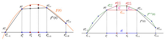
Figure 2. Left: the orange solid line ($f\left(t\right)$) is a polynomial function through $P_{i-1}^k,P_i^k,P_{i+1}^k,P_{i+2}^k$, and the piecewise broken line ($f^k\left(t\right)$) is a line through $P_{i-1}^k,P_i^k,P_{i+1}^k,P_{i+2}^k$. Right: insertion of the new points ($P_{3i+1}^{k+1}$ and $P_{3i+2}^{k+1}$).

Theorem 1. 

The NUFTCS scheme is convergent.

Proof of Theorem 1. 

In order to prove this conclusion, a continuous function ($f\left(t\right)$) is introduced. $\left\{P_{i-1}^k,P_i^k,P_{i+1}^k,P_{i+2}^k\right\}$ on the curve is associated with $f\left(t\right)$. Let $f\left(t\right)$ be a cubic polynomial generated by nodes $\left\{t_{i-1}^k,t_i^k,t_{i+1}^k,t_{i+2}^k\right\}$; then,

$$\begin{gathered} f\left(t\right)=f\left(t_i^k\right)+f\left[t_i^k,t_{i+1}^k \right]\left(t-t_i^k\right)+f\left[t_i^k,t_{i+1}^k,t_{i+2}^k \right]\left(t-t_i^k\right)\left(t-t_{i+1}^k\right) \\ +f\left[t_{i-1}^k,t_i^k,t_{i+1}^k,t_{i+2}^k \right]\left(t-t_{i-1}^k\right)\left(t-t_i^k\right)\left(t-t_{i+1}^k\right). \end{gathered}$$

Constructing $f^k\left(t\right)=f\left(t_i^k\right)+f\left[t_i^k,t_{i+1}^k \right]\left(t-t_i^k\right)$ as the chord passing through $P_i^k$ and $P_{i+1}^k$ yields

$$\begin{array}{c}\hspace{1em}\hspace{1em}\hspace{1em}\hspace{1em}f\left(t\right)-f^k\left(t\right)\\ \hspace{1em}\hspace{1em}\hspace{1em}\hspace{1em}\hspace{1em}\hspace{1em}=f\left[t_i^k,t_{i+1}^k,t_{i+2}^k \right]\left(t-t_i^k\right)\left(t-t_{i+1}^k\right)+f\left[t_{i-1}^k,t_i^k,t_{i+1}^k,t_{i+2}^k\right]\left(t-t_{i-1}^k\right)\left(t-t_i^k\right)\left(t-t_{i+1}^k\right)\\ =\frac{\left(t-t_i^k\right)\left(t-t_{i+1}^k\right)}{t_{i+2}^k-t_{i-1}^k}\left\{f\left[t_i^k,t_{i+1}^k,t_{i+2}^k\right]\left(t-t_{i-1}^k\right)+f\left[t_{i-1}^k,t_i^k,t_{i+1}^k \right]\left(t_{i+2}^k-t\right)\right\}.\end{array}$$

where $f\left[t_{i-1}^k,t_i^k,t_{i+1}^k,t_{i+2}^k \right]=\frac{f\left[t_i^k,t_{i+1}^k,t_{i+2}^k \left]+f\right[t_{i-1}^k,t_i^k,t_{i+1}^k\right]}{t_{i+2}^k-t_{i-1}^k}$.

Substituting $t_1^{*}=\frac{2t_i+t_{i+1}}{3}$ into $f\left(t\right)$ and $f^k\left(t\right)$ yields

$$\begin{array}{c}f\left(t_1^{*}\right)-f^k\left(t_1^{*}\right)=-\frac{2{\left(t_{i+1}^k-t_i^k\right)}^2}{9\left(t_{i+2}^k-t_{i-1}^k\right)} \times \\ \left\{f\left[t_i^k,t_{i+1}^k,t_{i+2}^k\right]\left(\frac{t_{i+1}^k-t_i^k}{3}+\left(t_i^k-t_{i-1}^k\right)\right) +f\left[t_{i-1}^k,t_i^k,t_{i+1}^k\right]\left(\frac{2\left(t_{i+1}^k-t_i^k\right)}{3}+\left(t_{i+2}^k-t_{i+1}^k\right)\right)\right\}.\end{array}$$

Let $a=\frac{t_i^k-t_{i-1}^k}{t_{i+1}^k-t_i^k}$, $b=\frac{t_{i+2}^k-t_{i+1}^k}{t_{i+1}^k-t_i^k}$; then,

$$f\left(t_1^{*}\right)-f^k\left(t_1^{*}\right)=-\frac{2{\left(t_{i+1}^k-t_i^k\right)}^2}{9\left(a+b+1\right)}\left\{f\left[t_i^k,t_{i+1}^k,t_{i+2}^k\right]\left(\frac{1}{3}+a\right)+f\left[t_{i-1}^k,t_i^k,t_{i+1}^k\right]\left(\frac{2}{3}+b\right)\right\}.$$

(6)

Let ${\stackrel{\rightharpoonup }{\lambda }}_i^k$ and ${\stackrel{\rightharpoonup }{\lambda }}_{i+1}^k$ be the vectors

$${\stackrel{\rightharpoonup }{\lambda }}_i^k=P_{3i+1}^{k+1}-\frac{2P_i^k+P_{i+1}^k}{3}, {\stackrel{\rightharpoonup }{\lambda }}_{i+1}^k=P_{3i+1}^{k+1}-\frac{P_i^k+2P_{i+1}^k}{3},$$

depicted in Figure 2 (right), and consider divided differences at $P_i^k$ and $P_{i+1}^k$,

$$P_i^{k,\left[1\right]}=\frac{P_i^k-P_{i-1}^k}{t_i^k-t_{i-1}^k}, P_{i+1}^{k,\left[1\right]}=\frac{P_{i+1}^k-P_i^k}{t_{i+1}^k-t_i^k}, P_i^{k,\left[2\right]}=\frac{P_i^{k,\left[1\right]}-P_{i-1}^{k,\left[1\right]}}{t_i^k-t_{i-1}^k}, P_{i+1}^{k,\left[2\right]}=\frac{P_{i+1}^{k,\left[1\right]}-P_i^{k,\left[1\right]}}{t_{i+1}^k-t_i^k}.$$

Combining (6), yields

$$\begin{array}{c}{\stackrel{\rightharpoonup }{\lambda }}_i^k=P_{3i+1}^{k+1}-\frac{2P_i^k+P_{i+1}^k}{3}=f\left(t_1^{*}\right)-f^k\left(t_1^{*}\right)\\ \hspace{1em}=-\frac{2{\left(t_{i+1}^k-t_i^k\right)}^2}{9\left(a+b+1\right)}\left\{P_i^{k,\left[2\right]}\left(\frac{1}{3}+a\right)+P_{i+1}^{k,\left[2\right]}\left(\frac{2}{3}+b\right)\right\}\\ \hspace{1em}=-\frac{2\left(t_{i+1}^k-t_i^k\right)}{9\left(a+b+1\right)}\left\{\left(\frac{a+1/3}{1+a}\left(P_{i+1}^{k,\left[1\right]}-P_i^{k,\left[1\right]}\right)\right)+\left(\frac{b+2/3}{1+b}\left(P_{i+2}^{k,\left[1\right]}-P_{i+1}^{k,\left[1\right]}\right)\right)\right\}.\end{array}$$

Because $\Vert P_i^{k,\left[1\right]}\Vert$ = 1 and $d_{i+1}^k=t_{i+1}^k-t_i^k$, let $a>b(>0)$; then,

$$\Vert {\stackrel{\rightharpoonup }{\lambda }}_i^k\Vert \le \frac{2d_{i+1}^k}{9\left(a+b+1\right)}\left(2\frac{a+1/3}{1+a}+2\frac{b+2/3}{1+b}\right)\le \frac{4}{9}\cdot \frac{d_{i+1}^k}{1+b}\le \frac{4}{9}{d}_{i+1}^k.$$

(7)

According to the definition of ${\stackrel{\rightharpoonup }{e}}_{i+1}^k$ and ${\stackrel{\rightharpoonup }{\lambda }}_i^k$, ${\stackrel{\rightharpoonup }{e}}_{i+1}^{k+1}=\frac{1}{3}{\stackrel{\rightharpoonup }{e}}_{i+1}^k+{\stackrel{\rightharpoonup }{\lambda }}_i^k$; then,

$$d_{i+1}^{k+1}= \Vert {\stackrel{\rightharpoonup }{e}}_{i+1}^{k+1}\Vert \le \frac{1}{3}\Vert {\stackrel{\rightharpoonup }{e}}_{i+1}^k\Vert + \Vert {\stackrel{\rightharpoonup }{\lambda }}_i^k\Vert =\frac{1}{3}{d}_{i+1}^k+\frac{4}{9}{d}_{i+1}^k=\frac{7}{9}{d}_{i+1}^k\le \cdots \le {\left(\frac{7}{9}\right)}^{k+1}{d}_{i+1}^0,$$

combined with Equation (7) yields $\underset{k\to +\infty }{\lim }\Vert {\stackrel{\rightharpoonup }{\lambda }}_i^k\Vert =0$.

Similarly, substituting $t_1^{*}=\frac{t_i+2t_{i+1}}{3}$ into $f\left(t\right)$ and $f^k\left(t\right)$ yields $\underset{k\to +\infty }{\lim }\Vert {\stackrel{\rightharpoonup }{\lambda }}_{i+1}^k\Vert =0$.

Because

$$\Vert f^{\left(k+1\right)} \left(t\right)-f^k\left(t\right){\Vert }_{\infty }=\underset{t\in R}{sup}\Vert f^{\left(k+1\right)} \left(t\right)-f^k\left(t\right)\Vert =\underset{t\in R}{sup}Max\left\{\Vert {\stackrel{\rightharpoonup }{\lambda }}_i^k\Vert , \Vert {\stackrel{\rightharpoonup }{\lambda }}_{i+1}^k\Vert \right\},$$

$$\underset{k\to +\infty }{\lim }\Vert f^{\left(k+1\right)} \left(t\right)-f^k\left(t\right){\Vert }_{\infty }=\underset{k\to +\infty }{lim}\underset{t\in R}{sup}Max\left\{\Vert {\stackrel{\rightharpoonup }{\lambda }}_i^k\Vert , \Vert {\stackrel{\rightharpoonup }{\lambda }}_{i+1}^k\Vert \right\}=0;$$

then, the scheme is convergent. □

Theorem 2. 

Let  $P={\left\{P_i^0 \right\}}_{i\in Z}$ be a set of initial points, between  $P_i^0,P_{i+1}^0,i\in Z$, the piecewise limit curve generated by NUFTCS is  $C^1$.

Proof of Theorem 2. 

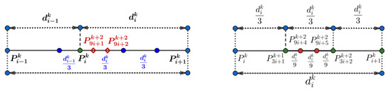
In the $k$-th refinement, the initial control points $P_i^0,P_{i+1}^0$ are replaced by $P_{3^{k}i}^k,P_{3^k\left(i+1\right)}^k,i\in Z$, and $P_{3^{k}i+j}^k,j=1,2,\cdots ,3^k-1$ is the new point generated by the subdivision scheme $\left(5\right)$. If $k=1$, the mask parameter to generate $P_{3i+1}^1$ and $P_{3i+2}^1$ is $\left[d_{i-1}^0,d_i^0,d_{i+1}^0\right]$, the mask is non-uniform, as shown in Figure 3 (left). If $k=2$, the mask parameter to generate $P_{9i+1}^2$ and $P_{9i+2}^2$ is $\left[\frac{d_{i-1}^0}{3},\frac{d_i^0}{3},\frac{d_i^0}{3}\right]$, so the mask is non-uniform too, but the mask parameter to generate $P_{9i+4}^2$ and $P_{9i+5}^2$ is $\left[\frac{d_i^0}{3},\frac{d_i^0}{3},\frac{d_i^0}{3}\right]$, so the mask is

$$\left\{\cdots ,0,0,-\frac{5}{81},-\frac{4}{81},0,\frac{10}{27},\frac{20}{27},1,\frac{20}{27},\frac{10}{27},0,-\frac{4}{81},-\frac{5}{81},0,0,\cdots \right\}.$$

Figure 3. After 1 subdivision, the update of the mask parameters of the subdivision (5). Left: the mask parameters to generate the $P_{9i+1}^2$ and $P_{9i+2}^2$. Right: the mask parameters to generate the $P_{9i+4}^2$ and $P_{9i+5}^2$.

Using the continuity proof method of uniform subdivision [11], the limit curve between points $P_i^0,P_{i+1}^0$ is $C^1$. □

Remark 1. 

The limit curve of the NUFTCS scheme is  $C^1$.

Proof of Remark 1. 

According to Theorems 1 and 2, the sequence $\left\{f^k\left(t\right),k\in N\right\}$ is a Cauchy sequence, and among $P_{i-1}^0, P_{i+1}^0$, and it uniformly converges to a piecewise differentiable function $f\left(t\right)$. Therefore, at point $P_i^0$, the limit curve of NUFTCS is $C^1$. Combination Theorem 2, in arbitrary points, the limit curve of NUFTCS scheme is $C^1$. □

3. Non-Uniform Local Ternary Interpolation Surface Subdivision (NULTISS) on Regular Quadrilateral Mesh

Regular mesh refers to a polyhedron shape consisting of points, edges, and surfaces among which the vertex $P_0$ is a three-dimensional space point with four and only four connected edges, i.e., $e_i,$i = 1,2,3,4. Each edge ($e_i$) is a straight-line segment connecting two vertices ($P_0,P_i, i=1,2,3,4$). Each surface ($S_i$) is composed of four edges, i.e., $e_i,$i = 1,2,3,4. Furthermore, each edge has two and only two connected faces, as shown in Figure 4 (left).

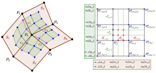
Figure 4. Left: notation for the initial mesh (consists of black dots ($P_0,P_i$), solid lines ($e_i$), and light-pink shaded quadrilateral faces ($S_i,i=1,2,3,4$)) and the new mesh after refinement (consists of $P_0$ new edge points (purple diamonds), new face points (blue dots), dotted lines, and light-green shaded quadrilateral faces). Right: the mask parameters of the interpolation points in the horizontal and vertical directions.

In regular quadrilateral meshes, as an advantageous alternative to tensor product construction, surface subdivision can better handle initial mesh with arbitrary topology. The purpose of this section is to naturally expand NUFTCS (5) to regular quadrilateral mesh and employ appropriate parameters to obtain a non-uniform surface subdivision scheme. Hereafter, this scheme is referred to as NULTISS (non-uniform local ternary interpolation surface subdivision).

3.1. Non-Uniform Parametric Surface Subdivision

Non-uniform parametric interpolation surface subdivision can be regarded as an iterative process. Let $M^k$ denote a kth lever regular quadrilateral mesh of 3D points; a mesh with new parameters ($M^{k+1}$) is generated according to the steps outlined below; for each refinement level $k\ge 1$, it

• Calculates the new edge points for each edge, as shown in Figure 4 (left; purple diamonds);
• Calculates the new surface points for each face, as shown in Figure 4 (left; blue dots);
• Constructs a new mesh, as shown in Figure 4 (left; light-green quadrangles).

• Creating new edges: Connecting new edge points on each edge, connecting new edge points with the “nearest” vertex, circularly connecting four new face points, and connecting new face points with the “nearest” new edge points;
• Create new faces: faces surrounded by four new edges.

Let $\left\{P_{i,j}^k, i, j\in \mathbb{Z}\right\}$ be the vertex set of the mesh ($M^k$), and $d_{i+1,j}^k=P_{i+1,j}^k-P_{i,j}^k, e_{i+1,j}^k=P_{i,j+1}^k-P_{i,j}^k$; accordingly, the mask parameters in the horizontal direction are ${\alpha }_{i,j}^k=\left[d_{i-1,j}^k, d_{i,j}^k, d_{i+1,j}^k\right]$ and ${\beta }_{i,j}^k=\left[d_{i+1,j}^k, d_{i,j}^k, d_{i-1,j}^k\right]$, whereas those in the vertical direction are ${\xi }_{i,j}^k=\left[e_{i,j-1}^k, e_{i,j}^k, e_{i,j+1}^k\right]$ and ${\eta }_{i,j}^k=\left[e_{i,j+1}^k, e_{i,j}^k, e_{i,j-1}^k\right]$, as shown in Figure 4 (right).

Using the curve subdivision scheme (5),

♦

Vertex points

$$P_{3i,3j}^{k+1}=P_{i,j}^k,$$

♦

Edge points

$$\left\{\begin{array}{c} P_{3i+1,3j}^{k+1}={\displaystyle \sum _{l=-1}^2}{a}_l\left({\alpha }_{i,j}^k\right)P_{i+l,j}^k, P_{3i+2,3j}^{k+1}={\displaystyle \sum _{l=-1}^2}{a}_l\left({\beta }_{i,j}^k\right)P_{i+l,j}^k,\\ P_{3i,3j+1}^{k+1}={\displaystyle \sum _{l=-1}^2}{a}_l\left({\xi }_{i,j}^k\right)P_{i,j+l}^k, P_{3i,3j+2}^{k+1}={\displaystyle \sum _{l=-1}^2}{a}_l\left({\eta }_{i,j}^k\right)P_{i,j+l}^k.\end{array}\right.$$

(8)

For the face points, using the idea of tensor product, we define an average parameterization as

$${\overline{d}}_i^k=\frac{{\displaystyle \sum _{j\in Z}}{d}_{i,j}^k }{\#\left\{d_{i,j}^k,j\in Z\right\}}, {\overline{e}}_i^k=\frac{{\displaystyle \sum _{i\in Z}}{e}_{i,j}^k }{\#\left\{e_{i,j}^k,i\in Z\right\}},$$

so that

$$\begin{gathered} {\overline{\alpha }}_i^k=\left[{\overline{d}}_{i-1}^k, {\overline{d}}_i^k, {\overline{d}}_{i+1}^k\right],\hspace{1em}{\overline{\beta }}_i^k=\left[{\overline{d}}_{i+1}^k, {\overline{d}}_i^k, {\overline{d}}_{i-1}^k\right], \\ {\overline{\xi }}_j^k=\left[{\overline{e}}_{j-1}^k, {\overline{e}}_j^k, {\overline{e}}_{j+1}^k\right],\hspace{1em}{\overline{\eta }}_i^k=\left[{\overline{e}}_{j+1}^k, {\overline{e}}_j^k, {\overline{e}}_{j-1}^k\right], \end{gathered}$$

are the mask parameters associated with the two mesh directions. Thus, the masks are calculated according to Equations (3) and (4), as shown in Figure 5 (Left).

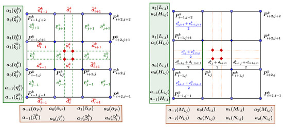
Figure 5. Mask parameterization of surface subdivision. Left: global non-uniform parameterization of surface subdivision Right: local non-uniform parameterization of surface subdivision.

♦

Face points

$$\left\{\begin{array}{c}{P}_{3i+1,3j+1}^{k+1}={\displaystyle \sum _{m=-1}^2}{\displaystyle \sum _{n=-1}^2}{a}_m({\overline{\alpha }}_i^k)a_n\left({\overline{\xi }}_j^k\right)P_{i+m,j+n}^k,\\ P_{3i+2,3j+1}^{k+1}={\displaystyle \sum _{m=-1}^2}{\displaystyle \sum _{n=-1}^2}{a}_m({\overline{\beta }}_i^k)a_n\left({\overline{\xi }}_j^k\right)P_{i+m,j+n}^k,\\ P_{3i+1,3j+2}^{k+1}={\displaystyle \sum _{m=-1}^2}{\displaystyle \sum _{n=-1}^2}{a}_m({\overline{\alpha }}_i^k)a_n\left({\overline{\eta }}_j^k\right)P_{i+m,j+n}^k,\\ P_{3i+2,3j+2}^{k+1}={\displaystyle \sum _{m=-1}^2}{\displaystyle \sum _{n=-1}^2}{a}_m({\overline{\beta }}_i^k)a_n\left({\overline{\eta }}_j^k\right)P_{i+m,j+n}^k.\end{array}\right.$$

(9)

3.2. Local Parametrization Surface Subdivision

Each subdivision step generates a refinement mesh with additional vertices, edges, and faces, as a consequence of which a suitable parameterization should be set in correspondence to the newly created edges. The method (tensor product) we choose to calculate the knot interval parameter (average parameter) affects the characteristics of the limit surface. In order to ensure that our subdivision rules can appropriately deal with non-uniform mesh, we propose a local parameterization method.

As shown in Figure 5 (right), when generating a new face point on a quadrilateral with $P_{i,j}^k,P_{i+1,j}^k,P_{i,j+1}^k,P_{i+1,j+1}^k$ as the vertex (the point may not be in the quadrilateral), in order to avoid the influence of “farther” points, we only consider the six parameters ($d_{i+k,j+l}^k,e_{i+k,j+l}^k,k=-1,0,1,l=0,1$) of the other four faces connected with one edge of the quadrilateral and adjust the parameters locally, resulting in a local subdivision scheme of the calculated face points.

As shown in Figure 5 (right), let

$${\tilde{d}}_{i,j}^k=\frac{d_{i,j}^k+d_{i,j+1}^k}{2},\hspace{1em}{\tilde{e}}_{i,j}^k=\frac{e_{i,j}^k+e_{i+1,j}^k}{2},$$

(10)

and four mask parameters in two directions are recorded as

$$\begin{gathered} M_{i,j}^k=\left\{{\tilde{d}}_{i-1,j}^k,\hspace{1em}{\tilde{d}}_{i,j}^k,\hspace{1em}{\tilde{d}}_{i+1,j}^k\right\}, N_{i,j}^k=\left\{{\tilde{d}}_{i+1,j}^k,\hspace{1em}{\tilde{d}}_{i,j}^k,\hspace{1em}{\tilde{d}}_{i-1,j}^k\right\}, \\ {H}_{i,j}^k=\left\{{\tilde{e}}_{i,j-1}^k,\hspace{1em}{\tilde{e}}_{i,j}^k,\hspace{1em}{\tilde{e}}_{i,j+1}^k\right\}, L_{i,j}^k=\left\{{\tilde{e}}_{i,j+1}^k,\hspace{1em}{\tilde{e}}_{i,j}^k,\hspace{1em}{\tilde{e}}_{i,j-1}^k\right\}, \end{gathered}$$

so that the face points can be calculation as

$$\left\{\begin{array}{c}{P}_{3i+1,3j+1}^{k+1}={{\displaystyle \sum }}_{m=-1}^2{{\displaystyle \sum }}_{n=-1}^2{a}_m\left(M_{i,j}^k\right)a_n\left(H_{i,j}^k\right)P_{i+m,j+n}^k,\hspace{1em}{P}_{3i+2,3j+1}^{k+1}={{\displaystyle \sum }}_{m=-1}^2{{\displaystyle \sum }}_{n=-1}^2{a}_m\left(N_{i,j}^k\right)a_n\left(H_{i,j}^k\right)P_{i+m,j+n}^k,\\ P_{3i+1,3j+2}^{k+1}={{\displaystyle \sum }}_{m=-1}^2{{\displaystyle \sum }}_{n=-1}^2{a}_m\left(M_{i,j}^k\right)a_n\left(L_{i,j}^k\right)P_{i+m,j+n}^k\hspace{1em}{P}_{3i+2,3j+2}^{k+1}={{\displaystyle \sum }}_{m=-1}^2{{\displaystyle \sum }}_{n=-1}^2{a}_m\left(N_{i,j}^k\right)a_n\left(L_{i,j}^k\right)P_{i+m,j+n}^k.\end{array}\right.$$

(11)

3.3. Convergence and Continuity of NULTISS

According to the mask calculation formula of curve subdivision, we refer to $d_i^k$ as the edge parameter. The mask parameter is composed of three adjacent edge parameters. Local parameterization surface subdivision is a non-stationary subdivision, and the mask changes with changes in the edge parameters. Furthermore, each subdivision generates a refined mesh with more vertices, edges, and surfaces. In order to analyze the shape of the limit surface according to the change rule of mask parameters, we redefine the vertex subscript and edge parameter subscript of the initial mesh, as indicated in Figure 6 (left and right) by the edge parameter subscript after two refinement steps.

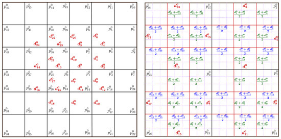
Figure 6. Left: vertex subscript and edge parameter subscript of the initial mesh. Right: edge parameter subscript after two refinement steps.

In particular, after one step of the subdivision algorithm, three different types of regions are identified (see Figure 7), which we call

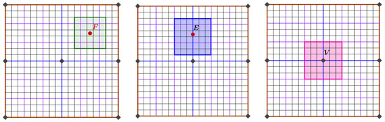
Figure 7. Three different types of regions. Left: the region surrounding the face point. Middle: the region surrounding the edge point. Right: the region surrounding the vertex.

• Tensor product regions, as shown in Figure 7 (left);
• Regions augmented across one edge, as shown in Figure 7 (middle);
• Regions augmented around a vertex, as shown in Figure 7 (right).

3.3.1. Parameter Updating Rules

(1)

Mask parameter updating rules for interior points in the region are generated by tensor product.

As shown in Figure 8 (left), let $P_0^0,P_1^0,P_2^0,P_{37}^0$ be the four vertices of an initial quadrilateral, and the parameters of its four edges are $d_1^0, d_5^0, d_3^0,d_{19}^0$. The points $F^1$ and $F^2$ are two face points on the refinement mesh generated after two subdivisions and three subdivisions, respectively. Because the subdivision scheme is a ternary interpolation subdivision, after $k$ subdivisions, the values of the edge parameters are $\frac{1}{3}$ of the average value of symmetrical edge parameters after $k-1$ subdivisions. According to Formula (8), the mask parameters in two directions used to generate $F^1$ are $[d_1^1,d_1^1,d_1^1$] and $\left[d_5^1,d_5^1,d_5^1\right]$, as shown in Figure 8 (left), where $d_1^1=\frac{d_1^0+d_3^0}{6}$ and $d_5^1=\frac{d_{18}^0+d_{19}^0}{6}$. According to mask computer Formulas (3) and (4), we can replace the mask parameters with [1, 1, 1] and [1, 1, 1], as shown in Figure 8 (right). Similarly, the mask parameters for $F^2$ are $\left[d_1^2,d_1^2,d_1^2\right]$ and $\left[d_5^2,d_5^2,d_5^2\right]$, as shown in Figure 8 (left), where $d_1^1=\frac{d_1^0+36d_3^0}{36}$ and $d_5^1=\frac{d_5^0+3d_{19}^0}{36}$ can also be replaced by $\left[1, 1, 1\right]$ and $\left[1, 1, 1\right]$, respectively.

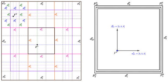
Figure 8. Updating of the mask parameters around the face point after two and three refinement steps. Left: the mask parameters of the face point $F^1$ and $F^2$. Right: according to (4), the mask parameters are replaced by $\left[1, 1, 1\right]$ and $\left[1, 1, 1\right]$.

Based on the above analysis, after several levels of refinement, for any point on the limit surface in the internal regions, the mask parameters that generate this point are uniform, as shown in Figure 8 (right).

(2)

Mask parameter updating rules for points in the region augmented across one edge

As shown in Figure 9, $P_0^0{P}_{19}^0$ and $P_0^0{P}_7^0$ are two initial edges connected with $P_0^0$. $E^1$ is the point in the regions augmented across edge $P_0^0{P}_{19}^0$, and $E^2$ is the point in the regions augmented across the edge $P_0^0{P}_7^0$, which were generated after two subdivisions and three subdivisions, respectively. The mask parameters in the two directions used to generate $E^1$ are $\left[d_{13}^1,d_1^1,d_1^1\right]$ and $\left[\frac{d_5^1+d_{19}^0}{2},\frac{d_5^1+d_{19}^0}{2},\frac{d_5^1+d_{19}^0}{2}\right]$, where $d_{13}^1=\frac{d_{13}^0+d_{23}^0}{2}$ and $d_1^1=\frac{d_1^0+d_3^0}{2}$. In a similar way, the second mask parameter can be changed to $\left[1, 1, 1\right]$. The mask parameters for $E^2$ are $\left[d_{13}^2,d_1^2,d_1^2\right]$ and $\left[1, 1, 1\right]$.

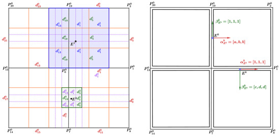
Figure 9. Updating of the mask parameters around the edge point after two subdivisions and three subdivisions. Left: after two subdivisions and three subdivisions, the mask parameters of $E^1$ and $E^2$. Right: the mask parameters after several subdivisions.

Based on the above analysis, it can be seen that for any point on the limit surface in the regions augmented across the edge, of the two mask parameters that generate this point, one is uniform and the other is non-uniform, as shown in Figure 9 (right).

(3)

Mask parameter updating rules for points in the region augmented around a vertex

As shown in Figure 10 (left), the initial mask parameters (${\alpha }_0^0$ and ${\beta }_0^0$) of $P_0^0$ are

$$\left[\frac{d_{13}^0+d_{23}^0}{2}, \frac{d_1^0+d_3^0}{2},\frac{d_1^0+d_3^0}{2}\right] \mathrm{and} \left[\frac{d_7^0+d_9^0}{2}, \frac{d_{19}^0+d_5^0}{2},\frac{d_{19}^0+d_5^0}{2}\right].$$

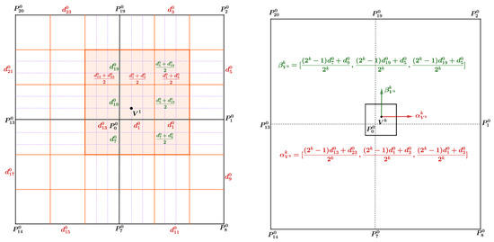
Figure 10. Left: updating of the mask parameters around the vertex after two subdivisions. Right: the mask parameters around the vertex after $k$ subdivisions.

$V^1$ is a face point generated after two subdivisions in the augmented region (Figure 10 (Left)) around vertex $P_0^0$. The mask parameters in two directions generated by Formula (10) are $\left[\frac{3d_{13}^0+d_{23}^0}{4}, \frac{3d_1^0+d_3^0}{4},\frac{3d_1^0+d_3^0}{4}\right]$ and $\left[\frac{3d_7^0+d_9^0}{4}, \frac{3d_{19}^0+d_5^0}{4},\frac{3d_{19}^0+d_5^0}{4}\right]$. If $V^k$ is a surface point generated after $k$ subdivisions, the mask parameters in the two directions (${\alpha }_0^k$ and ${\beta }_0^k$) for $V^k$ are

$$\left[\frac{\left(2^k-1\right)d_{13}^0+d_{23}^0}{2^k}, \frac{\left(2^k-1\right)d_1^0+d_3^0}{2^k},\frac{\left(2^k-1\right)d_1^0+d_3^0}{2^k}\right] \mathrm{and} \left[\frac{\left(2^k-1\right)d_7^0+d_9^0}{2^k}, \frac{\left(2^k-1\right)d_{19}^0+d_5^0}{2^k},\frac{\left(2^k-1\right)d_{19}^0+d_5^0}{2^k}\right],$$

as shown in Figure 10 (right).

3.3.2. Convergence and Continuity of NULTISS

In order to analyze the continuity of the limit surface, we first divide it into three patches, as shown in Figure 11 (left):

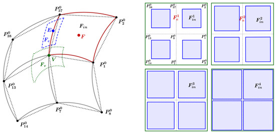
Figure 11. Three kinds of patches of the limit surface. Left: three types of limit surface. Right: the schematic diagram of the tensor product regions after 1, 2, 3 and 4 subdivisions.

• The surface patch corresponding to the tensor product region (denoted by $F_{in}$, i.e., the internal region surrounded by red solid lines);
• The surface patch corresponding to the region augmented across one edge (denoted by $F_e$, i.e., the internal region surrounded by blue dotted lines);
• The surface patch corresponding to the region augmented around a vertex (denoted by $F_v$, i.e., the internal region surrounded by green dotted lines).

Figure 11 (right) shows the change in patches $F_{in}$ and $F_e$ upon subsequent subdivisions; during the subdivision process, patch $F_{in}$ expands to the region corresponding to the initial quadrilateral, and patch $F_e$ shrinks to a curve (denoted by $F_e\backslash F_{in}$) corresponding to the initial edge.

Theorem 3. 

For any point ($F$) inside of  $F_{in}$, NULTISS generates a  $C^1$-continuous limit surface at this point.

Proof of Theorem 3. 

Based on the analysis presented in Section 3.3.1 (1), we can see that the mask parameters in two directions from a point ($F$) are uniform after several subdivisions. Thus, in these regions, the scheme converges to the tensor product surface generated by a $C^1$ uniform four-point ternary scheme so that the limit surface at $F$ is $C^1$ continuous. □

Theorem 4. 

For any point ($E$) inside of  $F_e\backslash F_{in}$, the limit surface generated at E by NULTISS is  $C^1$ continuous.

Proof of Theorem 4. 

On the one hand, according to the analysis presented in Section 3.3.1 (2), the mask parameters for point $E$ in one direction (along the direction of the intersection of two inner surfaces) are uniform, so $F_e\backslash F_{in}$ is a limit curve obtained by a uniform four-point ternary subdivision scheme. On the other hand, this curve is the intersection of two $C^1$ continuous surface patches corresponding to two adjacent initial quadrilaterals. Accordingly, for any point ($E$) inside of $F_e\backslash F_{in}$, the limit surface generated at this point by NULTISS is $C^1$ continuous. □

What follows is proof of the convergence and continuity of the limit surface at the vertex.

In this paper, the Lagrange interpolation basis function ($L_i\left(t\right),i=-1,0,1,2$) is used to obtain the mask. Because $L_i\left(t\right)$ is a cubic polynomial function, at any closed interval ($\left[a,b\right]$), it is bounded and Lipschitz continuous; then, for any $t_1,t_2\in ℝ$, there exists a constant $M>0$ independent of $a, b$. Accordingly,

$$\left|L_i\left(t_1\right)-L_i\left(t_2\right)\right|\le M\left(t_1-t_2\right).$$

Non-uniform tensor product stationary subdivision method: $V_0$ is the initial vertex, and ${\alpha }_0=\left[a,b,b\right]$ and ${\beta }_0=\left[c,d,d\right]$ are the initial mask parameters; therefore, according to Formulas (3) and (4), we can obtain the mask ($a_l\left({\alpha }_0\right),a_l\left({\beta }_0\right),l=-1, 0, 1, 2$). Let $V_1^k$ (as $P_{3i+1,3j+1}^k$) be the face points on the surface obtained after $k$ subdivisions; the mask for $V_1^k$ is still $a_l\left({\alpha }_0\right),a_l\left({\beta }_0\right)$. It can be easily observed that the mask is independent of level $k$, and this operator is a stationary subdivision operator on the initial mesh. Let the parameter in the horizontal direction of $V_0$ be $t_{0,x}$ and that in the vertical direction be $t_{0,y}$; then, the parameters of $V_1^k$ are denoted by $t_{1,x}^k$, $t_{1,y}^k$, and $t_{1,x}^k=t_{0,x}+\frac{b}{3^k}$, $t_{1,y}^k=t_{0,y}+\frac{d}{3^k}$. Thus, the mask for $V_1^k$ can be expressed as

$$a_l({\alpha }_1^k)=a_l \left({\alpha }_0\right)=L_l\left(t_{1,x}^k\right), a_l\left({\beta }_1^k\right)=a_l\left({\beta }_0\right)=L_l\left(t_{1,y}^k\right), l=-1, 0, 1, 2.$$

Non-uniform tensor product non-stationary subdivision method: Assume that $V_2^k$ is a face with points generated after $k$ subdivision by NULTISS. The mask parameters for $V_2^k$ are denoted by ${\alpha }_2^k$ and ${\beta }_2^k$ according to the instructions (3) presented in Section 3.3.1. Then, ${\alpha }_2^k=\left[a+\frac{A}{2^k},b+\frac{B}{2^k},b+\frac{B}{2^k}\right]$, ${\beta }_2^k=\left[c+\frac{C}{2^k},d+\frac{D}{2^k},d+\frac{D}{2^k} \right]$, where $A,B,C,D\in ℝ$. The horizontal direction parameter for $V_2^k$ is denoted by $t_{2,x}^k$; then, $t_{2,x}^k=t_{0,x}+\frac{b}{3^k}+\frac{B}{3·2^k}$. The vertical direction parameter is denoted by $t_{2,y}^k$; then, $t_{2,y}^k=t_{0,y}+\frac{d}{3^k}+\frac{D}{3·2^k}$. Therefore, the mask used to compute $V_2^k$ can be expressed as $a_i({\alpha }_2^k)=L_i\left(t_{2,x}^k\right)$, $a_i\left({\beta }_2^k\right)=L_i\left(t_{2,y}^k\right)$.

• If $t_{1,x}^k,t_{2,x}^k\in I_x≔\left[0,max\left\{a+2b,a+2b+\frac{A}{2}+B\right\}\right]$, then

  $$\left|a_i\left({\alpha }_2^k\right)-a_i\left({\alpha }_1^k\right)\right|=\left|L_i\left(t_{2,x}^k\right)-L_i\left(t_{1,x}^k\right)\right|\le M_1·\frac{\left|B\right|}{3·2^k},$$

  where $M_1$ is a constant independent of $k$.
• If $t_{1,y}^k,t_{2,y}^k\in I_y≔\left[0,max\left\{c+2d,c+2d+\frac{C}{2}+D\right\}\right]$, then

  $$\left|a_i\left({\beta }_2^k\right)-a_i\left({\beta }_1^k\right)\right|=\left|L_i\left(t_{2,y}^k\right)-L_i\left(t_{1,y}^k\right)\right|\le M_2·\frac{\left|D\right|}{3·2^k},$$

  where $M_2$ is a constant independent of $k$.

Theorem 5. 

At any point ($V$) in the augmented region of the initial vertex, the local matrix operator ($M_2^k=\left(m_{i,j}^2\right)$) of NULTISS is asymptotically equivalent to the local matrix operator ($M_1=\left(m_{i,j}^1\right)$) of the non-uniform tensor product stationary subdivision scheme.

Proof of Theorem 5. 

Let $V_1^k$ be a point generated by non-uniform stationary tensor product surface subdivision and $V_2^k$ be the point generated by NULTISS; therefore,

$$\begin{gathered} V_1^k={{\displaystyle \sum }}_{s=-1}^2{{\displaystyle \sum }}_{l=-1}^2{a}_s\left({\alpha }_1^k\right)a_l\left({\beta }_1^k\right)P_{i+s,j+l}^{k-1}={{\displaystyle \sum }}_{s=-1}^2{{\displaystyle \sum }}_{l=-1}^2{L}_s\left(t_{1,x}^k\right)L_l\left(t_{1,y}^k\right)P_{i+s,j+l}^{k-1}, \\ {V}_2^k={{\displaystyle \sum }}_{s=-1}^2{{\displaystyle \sum }}_{l=-1}^2{a}_s\left({\alpha }_2^k\right)a_l\left({\beta }_2^k\right)P_{i+s,j+l}^{k-1}={{\displaystyle \sum }}_{s=-1}^2{{\displaystyle \sum }}_{l=-1}^2{L}_s\left(t_{2,x}^k\right)L_l\left(t_{2,y}^k\right)P_{i+s,j+l}^{k-1}. \end{gathered}$$

We obtain

$$\begin{array}{c}{V}_1^k-V_2^k\\ ={{\displaystyle \sum }}_{s=-1}^2{{\displaystyle \sum }}_{l=-1}^2{L}_s\left(t_{1,x}^k\right)L_l\left(t_{1,y}^k\right)P_{i+s,j+l}^{k-1}-{{\displaystyle \sum }}_{s=-1}^2{{\displaystyle \sum }}_{l=-1}^2{L}_s\left(t_{2,x}^k\right)L_l\left(t_{2,y}^k\right)P_{i+s,j+l}^{k-1}\\ ={{\displaystyle \sum }}_{s=-1}^2\{{{\displaystyle \sum }}_{l=-1}^2[L_s\left(t_{1,x}^k\right)L_l\left(t_{1,y}^k\right)-L_s\left(t_{2,x}^k\right)L_l\left(t_{2,y}^k\right)]P_{i+s,j+l}^{k-1}\}\\ ={{\displaystyle \sum }}_{s=-1}^2\{{{\displaystyle \sum }}_{l=-1}^2[L_l\left(t_{1,y}^k\right)(L_s\left(t_{1,x}^k\right)-L_s\left(t_{2,x}^k\right))-L_s\left(t_{2,x}^k\right)(L_l\left(t_{2,y}^k\right)-L_l\left(t_{1,y}^k\right))]P_{i+s,j+l}^{k-1}\}, \end{array}$$

therefore,

$$\begin{array}{c}{{\displaystyle \sum }}_j|m_{i,j}^1-m_{i,j}^2|\\ =\left|{{\displaystyle \sum }}_{s=-1}^2\right\{{{\displaystyle \sum }}_{l=-1}^2[L_l\left(t_{1,y}^k\right)(L_s\left(t_{1,x}^k\right)-L_s\left(t_{2,x}^k\right))-L_s\left(t_{2,x}^k\right)(L_l\left(t_{2,y}^k\right)-L_l\left(t_{1,y}^k\right))]\}\\ \le {{\displaystyle \sum }}_{s=-1}^2\{{{\displaystyle \sum }}_{l=-1}^2[L_l\left(t_{1,y}^k\right)|L_s\left(t_{1,x}^k\right)-L_s\left(t_{2,x}^k\right)|+L_s\left(t_{2,x}^k\right)|L_l\left(t_{2,y}^k\right)-L_l\left(t_{1,y}^k\right)|]\}\\ \le {{\displaystyle \sum }}_{s=-1}^2{{\displaystyle \sum }}_{l=-1}^2[L_l\left(t_{1,y}^k\right)·M_1·\frac{\left|B\right|}{3·2^k}+L_s\left(t_{2,x}^k\right)·M_2·\frac{\left|D\right|}{3·2^k}].\end{array}$$

Let $M=max\left\{M_1·\left|B\right|,M_2·\left|D\right|\right\}$; the,

$${{\displaystyle \sum }}_j\left|m_{i,j}^1-m_{i,j}^2 \right|\le \frac{M}{3·2^k}{{\displaystyle \sum }}_{s=-1}^2{{\displaystyle \sum }}_{l=-1}^2[L_l\left(t_{1,y}^k\right)+L_s\left(t_{2,x}^k\right)]=\frac{M}{3·2^k}.$$

So

$${{\displaystyle \sum }}_{k\in Z}\Vert M_2^k-M_1{\Vert }_{\infty }=Ma{x}_i{{\displaystyle \sum }}_j\left|m_{i,j}^1-m_{i,j}^2 \right|\le \frac{M}{3·2^k} .$$

This concludes the proof. □

Theorem 6. 

The NULTISS rule generates a$C^1$continuous limit surface at any point.

Proof of Theorem 6. 

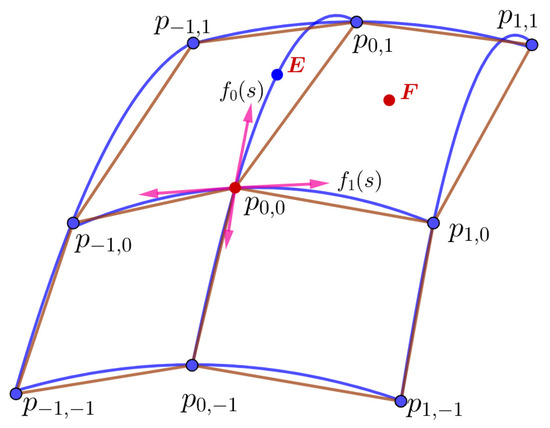
As shown in Figure 12, Theorem 3 shows that within the initial surface patch, any point ($F$) on the limit surface is $C^1$ continuous, and four surface patches surrounded by nine vertices $P_{i,j}^0,i,j=-1,0,1$ are continuous.

Figure 12. Notations for the continuous proof at a regular vertex.

According to Theorem 4, at any point ($E$) on the intersection curves ($f_0\left(s\right), f_1\left(s\right)$), the limit surface is $C^1$ continuous.

Theorem 5 shows that the local matrix operator of NULTISS at the initial vertex is asymptotically equivalent to the local matrix operator of the non-uniform tensor product scheme. Because the limit curve of four-point ternary curve subdivision is $C^1$ continuous, the limit surface generated by the tensor product is also $C^1$ continuous, so the limit surface of NULTISS is also $C^1$ continuous at the vertex.

Synthesis of the above points shows that the limit surface is $C^1$ continuous at any point. □

4. NULTISS on Irregular Quadrilateral Mesh

4.1. Construction Method of Virtual Points

Let $p_j^0$ be an extraordinary point with valance $n$; $\{p_j^{1,k},k=1,2,\cdots ,n\}$ is a set of edge points connected to $p_j^0$, $\{q_j^{1,k},k=1,2,\cdots ,n\}$ is the set of vertex points symmetrical to $p_j^0$ on the quadrilateral mesh, and $d_j^{1,k}= \Vert p_j^{1,k}-p_j^0\Vert$, ${\tilde{d}}_j^{1,k}= \Vert q_j^{1,k}-p_j^0\Vert$, as shown in Figure 13.

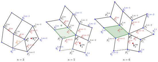
Figure 13. Notations for the construction of virtual points at an extraordinary point.

To compute the edge points on the $m$-th edge ($p_j^0{p}_j^m$) according to Formula (8) and the face points in the $m$-th quadrilateral region according to Formula (11), we need to find a virtual point ($V_j^m$) similar to the method described in [3]. Therefore, let

$$\begin{gathered} V_j^m=\frac{1}{A}\left[\frac{4}{n} {\displaystyle \sum }_{k=1}^n\left(d_j^{1,m-3+k}\cdot p_j^{1,1,m-3+k}\right)-{\displaystyle \sum }_{l=-1}^1{d}_j^{1,m+l}\cdot p_j^{1,m+l}\right] \\ +B\left[\frac{4}{n}{\displaystyle \sum }_{k=1}^n{\tilde{d}}_j^{m-3+k}\cdot p_j^{m-3+k}-{\displaystyle \sum }_{l=-2}^1{\tilde{d}}_j^{1,m+l}\cdot q_j^{1,m+l}\right], \end{gathered}$$

(12)

where

$$A={{\displaystyle \sum }}_{k=1}^n\frac{4d_j^{1,m-3+k}}{n}-d_j^{1,m-1}-d_j^{1,m}-d_j^{1,m+1},$$

and

$$B=-\frac{{\left(d_j^{1,m}\right)}^2\left(d_j^{1,m}+d_j^{1,m-2}\right)}{\left(d_j^{2,m}+d_j^{1,m}\right)\left(3d_j^{2,m}+d_j^{1,m}\right)\left(d_j^{2,m}+d_j^{1,m}+d_j^{1,m-2}\right)}.$$

Note: if $n=4$, then $V_j^m=p_j^{m-2}$.

4.2. Construction of New Edge Points and Face Points of the Extraordinary Point

As show in Figure 14 (Left), assume that $p_j^0 p_j^{1,m}$ is the $m$-th edge of the extraordinary point ($p_j^0$). $V_j^{m,0}$ is the initial virtual point calculated by (12) (Figure 14 (right)). The initial chordal parameter is denoted by $d_j^{0,m}= \Vert V_j^{m,0}-p_j^0\Vert$, and the initial mask parameters are denoted as

$${\alpha }_j^{m,0}=\left[d_j^{2,m},d_j^{1,m},d_j^{0,m}\right], {\beta }_j^{m,0}=\left[d_j^{0,m},d_j^{1,m},d_j^{2,m}\right].$$

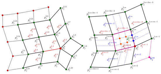
Figure 14. Notations for the construction of new edge points and face points at the extraordinary point. Left: an initial control mesh, where $p_j^0$ is the extraordinary point. Right: By generating virtual point $V_j^m$, irregular quadrilateral mesh is transformed into regular mesh.

Then, the mask parameters of the $k$th subdivision are

$${\alpha }_j^{m,k}=\left[d_j^{2,m,k},d_j^{1,m,k},d_j^{0,m,k}\right], {\beta }_j^{m,k}=\left[d_j^{0,m,k},d_j^{1,m,k},d_j^{2,m,k}\right],$$

Therefore, the new edge points (blue points, as shown in Figure 14 (right)) in the $k+1$-th subdivision scheme can be computed as

$$\left\{\begin{array}{c}{p}_j^{2,m,k+1}=a_{-1}\left({\alpha }_j^{m,k}\right)p_j^{2,m,k}+a_0\left({\alpha }_j^{m,k}\right)p_j^{1,m,k}+a_1\left({\alpha }_j^{m,k}\right)p_j^0+a_2\left({\alpha }_j^{m,k}\right)V_j^{m,k},\\ p_j^{1,m,k+1}=a_{-1}\left({\beta }_j^{m,k}\right)p_j^{2,k}+a_0\left({\beta }_j^{m,k}\right)p_j^{1,m,k}+a_1\left({\beta }_j^{m,k}\right)p_j^0+a_2\left({\beta }_j^{m,k}\right)V_j^{m,k}.\end{array}\right.$$

Let

$${\overline{d}}_j^{2,m+1,k}=\frac{d_j^{2,m+1,k}+d_j^{2,n+4m-1,k}}{2}, {\overline{d}}_j^{1,m+1,k}=\frac{d_j^{1,m+1,k}+d_j^{1,n+2m-1,k}}{2}, {\overline{d}}_j^{1,m-1,k}=\frac{d_j^{1,m-1,k}+d_j^{1,n+2m-2,k}}{2},$$

and

$${\overline{d}}_j^{1,m+2,k}=\frac{d_j^{1,m+2,k}+d_j^{1,n+2m+1,k}}{2}, {\overline{d}}_j^{1,m,k}=\frac{d_j^{1,m,k}+d_j^{1,n+2m,k}}{2}, {\overline{d}}_j^{2,m,k}=\frac{d_j^{2,m}+d_j^{2,n+4m-2,k}}{2}.$$

For the chordal parameter after $k$ subdivisions, the mask parameters of $\left(k+1\right)$th subdivision are

$$\begin{gathered} {\alpha }_j^{m,k}=\left[{\overline{d}}_j^{2,m+1,k},{\overline{d}}_j^{1,m+1,k},{\overline{d}}_j^{1,m-1,k}\right], {\beta }_j^{m,k}=\left[{\overline{d}}_j^{1,m-1,k},{\overline{d}}_j^{1,m+1,k},{\overline{d}}_j^{2,m+1,k}\right], \\ {\xi }_j^{m,k}=\left[{\overline{d}}_j^{1,m+2,k},{\overline{d}}_j^{1,m,k},{\overline{d}}_j^{2,m,k}\right], {\eta }_j^{m,k}=\left[{\overline{d}}_j^{2,m,k},{\overline{d}}_j^{1,m,k},{\overline{d}}_j^{1,m+2,k}\right], \end{gathered}$$

And the new face points in the $\left(k+1\right)$th subdivision can be computed as

$$\begin{gathered} p_j^{2,n+m,k+1}=\overrightarrow{a}\left({\alpha }_j^{m,k}\right)\cdot A\cdot \overrightarrow{a}{\left({\xi }_j^{m,k}\right)}^T, p_j^{2,n+3m,k+1}=\overrightarrow{a}\left({\beta }_j^{m,k}\right)\cdot A\cdot \overrightarrow{a}{\left({\xi }_j^{m,k}\right)}^T, \\ {p}_j^{2,n+3m-2,k+1}=\overrightarrow{a}\left({\alpha }_j^{m,k}\right)\cdot A\cdot \overrightarrow{a}{\left({\eta }_j^{m,k}\right)}^T, p_j^{2,n+3m-1,k+1}=\overrightarrow{a}\left({\beta }_j^{m,k}\right)\cdot A\cdot \overrightarrow{a}{\left({\eta }_j^{m,k}\right)}^T. \end{gathered}$$

where $\overrightarrow{a}\left(\ast \right)=\left[a_{-1}\left(\ast \right),a_0\left(\ast \right),a_1\left(\ast \right),a_2\left(\ast \right)\right]$ is the mask,

$$A=\left(\begin{array}{cccc}{p}_j^{2,n+3m-1,k}& p_j^{2,n+3m-2,k}& p_j^{2,m,k}& p_j^{2,n+3m-3,k}\\ p_j^{2,n+3m,k}& p_j^{1,n+m,k}& p_j^{1,m,k}& p_j^{1,n+m-1,k}\\ p_j^{2,m+1,k}& p_j^{1,m+1,k}& p_j^0& p_j^{1,m-1,k}\\ p_j^{2,n+3m+1,k}& p_j^{1,n+m+1,k}& p_j^{1,m+2,k}& V_j^{0,0,k}\end{array}\right).$$

4.3. The Continuity of NULTISS at the Extraordinary Point

Because the method proposed in this paper is parametric and non-uniform, it is difficult to analyze the characteristics of the subdivision matrix at an extraordinary point. According to the method described in [16], we provide a numerical analysis below using specific examples.

At the extraordinary point ($P_i^k$) obtained after $k$ subdivisions, let ${\stackrel{\rightharpoonup }{v}}_{i,j}^k$ be the normal vector of the plane determined by $P_i^k$ and the adjacent points ($P_{i,j}^k$, $P_{i,j+1}^k$), as shown in Figure 15, i.e.,

$${\stackrel{\rightharpoonup }{v}}_{i,j}^k=\stackrel{\rightharpoonup }{P_i^k{P}_{i,j}^k}\times \stackrel{\rightharpoonup }{P_i^k{P}_{i,j+1}^k}.$$

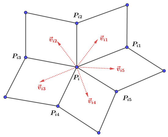
Figure 15. The normal vectors at the extraordinary point.

The angle ${\theta }_{i,j}^k$ of the two vectors ${\stackrel{\rightharpoonup }{v}}_{i,j}^k$ and ${\stackrel{\rightharpoonup }{v}}_{i,j+1}^k$ can be calculated as

$${\theta }_{i,j}^k=\arccos \frac{\left|{\stackrel{\rightharpoonup }{v}}_{i,j}^k\cdot {\stackrel{\rightharpoonup }{v}}_{i,j+1}^k\right|}{\Vert {\stackrel{\rightharpoonup }{v}}_{i,j}^k\Vert \cdot \Vert {\stackrel{\rightharpoonup }{v}}_{i,j+1}^k\Vert },$$

where ${\theta }_i^k=\underset{1\le j\le n}{max}{\theta }_{i,j}^k$ is the maximum angle of normal vectors at point $P_i^k$, and $n$ is the valance of $P_i^k$.

We assumed an initial mesh with the largest angle between the normal vectors for the experiments. The initial mesh is the nail with cross-shape mesh, and the vertices with valances of 3, 5, and 6 were tested after $k$ subdivisions. The result is shown in Table 1. All our experimentation shows that the limit surfaces are $G^1$ at the extraordinary points.

Table 1. The maximum angle between normal vectors of the extraordinary points with different valances.

$\mathbf{Valance} \mathbf{of} \mathit{n}$	$\mathit{k}=0$	$\mathit{k}=1$	$\mathit{k}=3$	$\mathit{k}=5$	$\mathit{k}=7$	$\mathit{k}=9$
$n=3$	1.5807	1.1219	0.6724	0.2132	0.0134	0.0062
$n=5$	1.5807	1.4567	0.9290	0.2614	0.0241	0.0035
$n=6$	1.5807	1.5628	1.0799	0.3132	0.0071	0.0021

5. Numerical Examples

5.1. Numerical Experiments on Subdivision with UNFTCS

We conclude by presenting some numerical experimentation in order to demonstrate the quality of NUFTCS limit curves, as shown in Figure 16. We randomly selected six control vertices on a unit circle and generated the limit curve using NUFTCS. The red curve is the limit curve generated by NUFTCS, and the green curve is the real curve (left). We applied NUFTCS to the curve control polygon of space with 40 points, and the limit curve is shown in Figure 16 (right).

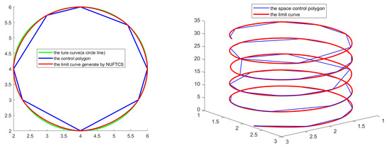
Figure 16. Subdivision curve with different control polygons. Left: planar control polygon (blue solid line); the red curve is the limit curve with NUFTCS, and the green curve is the real curve. Right: the space control polygon with 40 points, and the limit curve of the space control polygon generated by NUFTCS.

5.2. Numerical Experiments on Subdivision with NULTISS on Regular Quadrilateral Mesh

Below, we provide two examples of the NULTISS limit surface, as shown in Figure 17 and Figure 18. The first is a tire with a regular but non-uniform quadrilateral mesh. After three subdivisions, the mesh is dense and has a good lighting effect. The second example is a mesh formed by taking some points on the sphere.

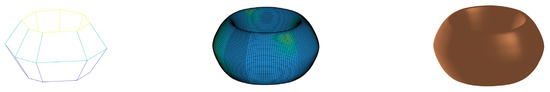
Figure 17. Subdivision surface of space with NULTISS. Left to right: initial mesh; mesh after three refinements; surface with lighting after three refinements.

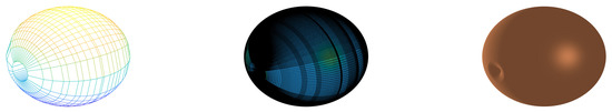
Figure 18. Subdivision surface of space with NULTISS. Left to right: initial mesh; mesh after two refinements; surface with lighting after three refinements.

5.3. Numerical Experiments on Subdivision with NULTISS on Irregular Quadrilateral Mesh

Below, we present an example of the NULTISS limit surface on irregular quadrilateral mesh, as shown in Figure 19. The model is a nail with a cross shape; the extraordinary points of the initial mesh of the model have three different valences, i.e., 3, 5, and 6; the chord length is refined twice, and an adequate mesh shape is obtained.

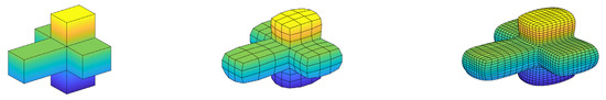
Figure 19. Subdivision surface of space with NULTISS. Left to right; initial mesh; mesh after one refinement; mesh after two refinements.

6. Discussion

In this paper, a novel method of curve subdivision based on non-uniform four-point ternary interpolation is proposed. Compared with uniform interpolation, the limit curve generated by our proposed method can avoid self-intersection and can effectively reflect the geometric characteristics of the control polygon. Moreover, using a tensor product, we also propose a non-uniform ternary surface subdivision scheme. In contrast to the method proposed in [16], this scheme has specific subdivision rules and formats on regular quadrilateral meshes, as well as mask calculation formula. In contrast to the method described in [15], we propose specific subdivision rules for extraordinary points. The effectiveness and superiority of our method are demonstrated by specific model examples.

Because subdivision rules are not limited by topology, we will further expand the application of the methods proposed in this paper in practical problems, such as point cloud reconstruction, grid optimization [28], etc. With respect to point cloud reconstruction, we will utilize point cloud compression technology, feature extraction technology, and a quadrilateral mesh generation method [29] to establish quadrilateral mesh, then use the method proposed in this paper to generate a limit surface.

References

- Catmull, E.; Clark, J. Recursively generated B-spline surfaces on arbitrary topological meshes. Comput. Aided Des. 1978, 10, 350–355. [Google Scholar] [CrossRef]
- Doo, D.; Sabin, M. Behaviour of recursive division surfaces near extraordinary points. Comput. Aided Des. 1978, 10, 356–360. [Google Scholar] [CrossRef]
- Kobbelt, L. Interpolatory subdivision on open quadrilateral nets with arbitrary topology. Comput. Graph. Forum 1996, 15, 400–410. [Google Scholar] [CrossRef]
- Li, G.; Ma, W. Interpolatory ternary subdivision surfaces. Comput. Aided Geom. Des. 2006, 23, 45–77. [Google Scholar] [CrossRef]
- Li, G.; Ma, W.; Bao, H. A New Interpolatory Subdivision for Quadrilateral Meshes. Comput. Graph. Forum 2005, 24, 3–16. [Google Scholar] [CrossRef]
- Loop, C. Smooth subdivision surfaces based on triangles. In Curve and Surface Fitting: Saint Malo; Cohen, A., Schumaker, L., Eds.; Nashboro Press: Brentwood, UK, 2002; Volume 12. [Google Scholar]
- Li, G.; Ma, W.; Bao, H. √2-Subdivision for quadrilateral meshes. Vis. Comput. 2004, 20, 180–198. [Google Scholar] [CrossRef]
- Kobbelt, L. √3-Subdivision. In Proceedings of the ACM Computer Graphics (Proceedings of SIGGRAPH ’2000), New Orleans, LA, USA, 23–28 July 2000; pp. 103–112. [Google Scholar]
- Ni, T.; Nasri, A.; Peters, J. Ternary subdivision for quadrilateral meshes. Comput. Aided Geom. Des. 2007, 24, 361–370. [Google Scholar] [CrossRef]
- Chaikin, G. An Algorithm for High-Speed Curve Generation. Comput. Graph. Image Process. 1974, 3, 346–349. [Google Scholar] [CrossRef]
- Dyn, N.; Levin, D.; Gregory, J. A four-point interpolatory subdivision scheme for curve design. Comput. Aided Geom. Des. 1987, 4, 257–268. [Google Scholar] [CrossRef]
- Dyn, N.; Levin, D. A butterfly subdivision scheme for surface interpolation with tension control. ACM Trans. Graph. 1990, 9, 160–169. [Google Scholar] [CrossRef]
- Sederberg, T.W.; Zheng, J.; Sewell, D.; Malcolm, S. Non-Uniform Recursive Subdivision Surfaces. In Proceedings of the ACM Computer Graphics (Proceedings of SIGGRAPH ’98), Orlando, FL, USA, 19–24 July 1998. [Google Scholar]
- Qin, K.; Wang, H. Continuity of non-uniform recursive subdivision surfaces. Sci. China Ser. E 2000, 5, 461–472. [Google Scholar]
- Beccari, C.; Casciola, G.; Romani, L. Non-uniform non-tensor product local interpolatory subdivision surfaces. Comput. Aided Geom. Des. 2013, 30, 357–373. [Google Scholar] [CrossRef]
- Li, X.; Chang, Y. Non-uniform interpolatory subdivision surface. Appl. Math. Comput. 2018, 324, 239–253. [Google Scholar] [CrossRef]
- Daubechies, I.; Guskov, I.; Sweldens, W. Regularity of irregular subdivision. Constr. Approx. 1999, 15, 381–426. [Google Scholar] [CrossRef]
- Lee, E. Choosing nodes in parametric curve interpolation. Comput. Aided Des. 1989, 21, 363–370. [Google Scholar] [CrossRef]
- Kuznetsov, E.; Yakimovich, A.Y. The best parameterization for parametric interpolation. J. Comput. Appl. Math. 2006, 191, 239–245. [Google Scholar] [CrossRef]
- Hussain, S.M.; Rehman, A.U.; Baleanu, D.; Nisar, K.S.; Ghaffar, A.; Abdul Karim, S.A. Generalized 5-Point Approximating Subdivision Scheme of Varying Arity. Mathematics 2020, 8, 474. [Google Scholar] [CrossRef]
- Beccari, C.; Casciola, G.; Romani, L. Non-uniform interpolatory curve subdivision with edge parameters built upon compactly supported fundamental splines. BIT Numer. Math. 2011, 51, 781–808. [Google Scholar] [CrossRef]
- Hassan, M.; Ivrissimitzis, I.; Dodgson, N.; Sabin, M. An interpolating 4-point C2 ternary stationary subdivision scheme. Comput. Aided Geom. Des. 2002, 19, 1–18. [Google Scholar] [CrossRef]
- Peng, K.; Tan, J.; Li, Z.; Zhang, L. Fractal behavior of a ternary 4-point rational interpolation subdivision scheme. Math. Comput. Appl. 2018, 23, 65. [Google Scholar] [CrossRef]
- Ashraf, P.; Nawaz, B.; Baleanu, D.; Nisar, K.S.; Ghaffar, A.; Khan, M.; Akram, S. Analysis of Geometric Properties of Ternary Four-Point Rational Interpolating Subdivision Scheme. Mathematics 2020, 8, 338. [Google Scholar] [CrossRef]
- Wang, H.; Kaihuai, Q. Improved Ternary Subdivision Interpolation Scheme. Tsinghua Sci. Technol. 2005, 10, 5. [Google Scholar] [CrossRef]
- Omar, M.; Khan, F. Generalized Subdivision Surface Scheme Based on 2D Lagrange Interpolating Polynomial and its Error Estimation. Commun. Math. Appl. 2018, 9, 447–458. [Google Scholar]
- Beccari, C.; Casciola, G.; Romani, L. Polynomial-based non-uniform interpolatory subdivision with features control. J. Comput. Appl. Math. 2011, 235, 4754–4769. [Google Scholar] [CrossRef]
- Jung, S.; Yoon, Y.T.; Huh, J.-H. An Efficient Micro Grid Optimization Theory. Mathematics 2020, 8, 560. [Google Scholar] [CrossRef]
- Zhu, J.Z.; Zienkiewicz, O.C.; Hinton, E.; Wu, J. A new approach to the development of automatic quadrilateral mesh generation. Int. J. Numer. Methods Eng. 1991, 32, 849–866. [Google Scholar] [CrossRef]
Disclaimer/Publisher’s Note: The statements, opinions and data contained in all publications are solely those of the individual author(s) and contributor(s) and not of MDPI and/or the editor(s). MDPI and/or the editor(s) disclaim responsibility for any injury to people or property resulting from any ideas, methods, instructions or products referred to in the content. |
© 2023 by the authors. Licensee MDPI, Basel, Switzerland. This article is an open access article distributed under the terms and conditions of the Creative Commons Attribution (CC BY) license (https://creativecommons.org/licenses/by/4.0/).