Dynamics of a Discrete Leslie–Gower Model with Harvesting and Holling-II Functional Response

Abstract

Recently, Christian Cortés García proposed and studied a continuous modified Leslie–Gower model with harvesting and alternative food for predator and Holling-II functional response, and proved that the model undergoes transcritical bifurcation, saddle-node bifurcation and Hopf bifurcation. In this paper, we dedicate ourselves to investigating the bifurcation problems of the discrete version of the model by using the Center Manifold Theorem and bifurcation theory, and obtain sufficient conditions for the occurrences of the transcritical bifurcation and Neimark–Sacker bifurcation, and the stability of the closed orbits bifurcated. Our numerical simulations not only illustrate corresponding theoretical results, but also reveal new dynamic chaos occurring, which is an essential difference between the continuous system and its corresponding discrete version.

1. Introduction and Preliminaries

The growth and relationship between species that coexist in the same environment can be modeled by a system of ordinary differential equations of the following form:

$$\dot{u}=f(u,\alpha ),$$

(1)

where $u\in R^n$, with $n\ge 1$, represents the species population size; $\alpha \in R^m$, with $m\ge 1$ and non-negative entries, is a parameter vector; and f: $\Omega$$\subset R^n$ × $R^m$ → $R^n$ is a continuous differentiable function. The mathematical analysis of Model (1) consists of determining all its possible dynamics, such as the existence and local stability of its equilibria, the existence of possible periodic trajectories, local bifurcation and global bifurcation by performing the variations on the parameter $\alpha$, etc. For related work, refer to [1,2] and the references cited therein.

In the past two decades, population biology has been greatly developed [3,4,5,6,7,8]. Ecologists are interested in mathematically describing the interaction and growth between two species, predator and prey, with equal probability of being consumed or captured and independence of their location. Assume that the growth of prey is subject to the carrying capacity $K\ge 0$ of the environment, the growth of the predator under the quality of the utilization of consumed prey $n\ge 0$ and the possible alternative food available $c\ge 0$ in the environment for new births. Then, a model describing the dynamics of prey $x(t)$ and predator $y(t)$ is given by

$$\left\{\begin{array}{c}\dot{x}=rx(1-{\displaystyle \frac{x}{K}})-{\displaystyle \frac{axy}{x+b}},\hfill \\ \dot{y}=sy(1-{\displaystyle \frac{y}{nx+c}}),\hfill \end{array}\right.$$

(2)

where $r,s\ge 0$ are the intrinsic growth rates of prey and predator, respectively. The predator functional response, which describes the change in the number of prey attacked by the predator in a unit of time, is described by a Holling-II type function $f(x)=\frac{ax}{x+b}$, with $a\ge 0$ is the maximum per capita consumption rate of the predator, and $b\ge 0$ is the semi-saturating rate of capture [9]. In particular, Model (2) follows the guidelines proposed by Leslie [10], which assume that the environmental carrying capacity to the predator should be proportional to the abundance of prey, and has become a basis to propose new models describing the behaviors between prey and predator [11,12,13,14,15,16,17,18].

Recently, Christian Cortés García [1] pointed out that by assuming that the predator can be harvested and the prey is protected from the predator if it is below the value $P>0$, Model (2) is modified to the following form:

$$\left\{\begin{array}{c}\dot{x}=rx(1-{\displaystyle \frac{x}{K}})-{\displaystyle \frac{ϵaxy}{x+b}},\hfill \\ \dot{y}=sy(1-{\displaystyle \frac{y}{ϵnx+c}})-qEy,\hfill \end{array}\right.$$

(3)

where $q>0$ is the catchability coefficient, $E>0$ the harvesting effort and

$$ϵ=\left\{\begin{array}{cc}1,\hfill & \mathrm{if}\mathrm{x}>\mathrm{P},\hfill \\ 0,\hfill & \mathrm{if}\mathrm{x}<\mathrm{P}.\hfill \end{array}\right.$$

We consider in this paper the case of x > P, and Model (3) is modified into

$$\left\{\begin{array}{c}\dot{x}=rx(1-{\displaystyle \frac{x}{K}})-{\displaystyle \frac{axy}{x+b}},\hfill \\ \dot{y}=sy(1-{\displaystyle \frac{y}{nx+c}})-qEy.\hfill \end{array}\right.$$

(4)

Model (4) was studied in [1], where it is mainly proved that Model (4) undergoes transcritical bifurcation, saddle-node bifurcation and Hopf bifurcation.

Generally speaking, it is impossible to obtain an exact solution for a complex differential equation system. So, many researchers derive the corresponding approximate solution by computer [19,20,21,22,23,24]. What the computer considers is the discrete points in the calculation process; so, the discrete model has practical significance in deriving the numerical solution. This motivates us to study the corresponding discrete model.

For a given continuous system, there are many different discrete methods, including the Euler forward difference scheme, the Euler backward difference scheme, the semi-discretization method, etc. Since the semi-discretization method does not need to consider the step size, one less parameter can be considered using this method, thus simplifying the calculation. So, in this paper, we use the semi-discretization method, which has been applied in many studies [25,26,27,28].

First, to facilitate later calculations, we can use the scaling $X={\displaystyle \frac{x}{K}}$, $Y={\displaystyle \frac{ay}{rK}}$ and $T=rt$ to non-dimensionalize System (4) to reduce the number of system parameters, and the dimensionless system obtained is as follows:

$$\left\{\begin{array}{c}{\displaystyle \frac{dX}{dT}}=X(1-X)-{\displaystyle \frac{XY}{X+j}},\hfill \\ {\displaystyle \frac{dY}{dT}}=fY-{\displaystyle \frac{gY}{X+h}},\hfill \end{array}\right.$$

(5)

in which

$$f={\displaystyle \frac{s-qE}{r}},g={\displaystyle \frac{s}{an}},h={\displaystyle \frac{c}{nK}},j={\displaystyle \frac{b}{K}}.$$

Notice that if $s\le qE$, it follows that System (5) only has trivial non-negative equilibria (0, 0) and (1, 0) because, from the second equation of System (5), one can see that $Y=0$. So, to avoid the trivial case, we always assume $s>qE$ in the sequel.

Next, we use the semi-discretization method to consider the discrete version of System (5). For this, suppose that $\left[T\right]$ denotes the greatest integer not exceeding T. Consider the average change rate of System (5) at integer number points

$$\left\{\begin{array}{c}\frac{1}{X(T)}\frac{dX(T)}{dT}=(1-X(\left[T\right]))-\frac{Y([T])}{X([T])+j},\hfill \\ \frac{1}{Y(T)}\frac{dY(T)}{dT}=f-\frac{g}{X([T])+h}.\hfill \end{array}\right.$$

(6)

It is easy to see that System (6) has piecewise constant arguments, and that a solution $(X(T),Y(T))$ of System (6) for $T\in [0,+\infty )$ possesses the following characteristics:

• On the interval $[0,+\infty )$, $X(T)$ and $Y(T)$ are continuous;
• When $T\in [0,+\infty )$, except possibly for the points $T\in \{0,1,2,3,\cdots \}$, $\frac{dX(T)}{dT}$ and $\frac{dY(T)}{dT}$ exist everywhere.

Integrating (6) over the interval [n,T] for any $T\in [n,n+1)$ and $n=0,1,2,\cdots$, one obtains the following system:

$$\left\{\begin{array}{c}X(T)=X_n{e}^{(1-X_n)-\frac{Y_n}{X_n+j}}(T-n),\hfill \\ Y(T)=Y_n{e}^{f-\frac{g}{X_n+h}}(T-n),\hfill \end{array}\right.$$

(7)

where $X_n=X(n)$ and $Y_n=Y(n)$.

Letting $T\to {(n+1)}^{-}$ in (7) leads to

$$\left\{\begin{array}{c}{X}_{n+1}=X_n{e}^{1-X_n-\frac{Y_n}{X_n+j}},\hfill \\ Y_{n+1}=Y_n{e}^{f-\frac{g}{X_n+h}},\hfill \end{array}\right.$$

(8)

where the parameters $f,g,h,j>0$ are the same as in System (5). In this paper, we mainly focus on the bifurcations of System (8).

The structure of the paper is as follows. In Section 2, we solve the fixed points of System (8), whose stability is obtained by using an important lemma. In Section 3, we derive the sufficient conditions for the occurrences of the transcritical bifurcation and Neimark–Sacker bifurcation and the stability of the closed orbits of System (8) bifurcated by using the Center Manifold Theorem and bifurcation theory. In Section 4, we present numerical simulations to illustrate corresponding theoretical results and reveal some new dynamics.

2. Existence and Stability of Fixed Points

In this section, we first consider the existence of the fixed points of System (8).

The fixed points of System (8) satisfy

$$X=X{e}^{1-X-\frac{Y}{X+j}},\left[5pt\right]Y=Y{e}^{f-\frac{g}{X+h}}.$$

Since System (8) is a biological system, we need to consider the biological significance of the system, and the fixed points we derive must be non-negative. By calculating, we find that System (8) has only four non-negative fixed points: one non-isolated fixed point $P_1=(0,Y_1)$ for $g=fh$ and any $Y_1>0$, and three isolated fixed points: $P_0=(0,0)$, $P_2=(1,0)$ and $P_3=(X_3,Y_3)$ for $fh<g<f(h+1)$, where

$$X_3=\frac{g-fh}{f},Y_3=(1-X_3)(X_3+j)=\frac{f(h+1)-g}{f}(\frac{g-fh}{f}+j).$$

The Jacobian matrix of System (8) at any fixed point $P(X,Y)$ takes the following form:

$$J(P)=\left(\begin{array}{cc}\left[1+X\left(\frac{Y}{{(X+j)}^2}-1\right)\right]e^{1-X-\frac{Y}{X+j}}& -\frac{X}{X+j}{e}^{1-X-\frac{Y}{X+j}}\\ \frac{gY}{{(X+h)}^2}{e}^{f-\frac{g}{X+h}}& e^{f-\frac{g}{X+h}}\end{array}\right).$$

The characteristic polynomial of the Jacobian matrix $J(P)$ reads

$$F(\lambda )={\lambda }^2-p\lambda +q,$$

where

$$\begin{array}{cc}\hfill p& =Tr(J(P))=\left[1+X\left(\frac{Y}{{(X+j)}^2}-1\right)\right]e^{1-X-\frac{Y}{X+j}}+e^{f-\frac{g}{X+h}},\hfill \\ \hfill q& =Det(J(P))=\left[1+X\left(\frac{Y}{{(X+j)}^2}-1\right)\right]e^{1-X-\frac{Y}{X+j}+f-\frac{g}{X+h}}\hfill \\ & +\frac{gXY}{(X+j){(X+h)}^2}{e}^{f-\frac{g}{X+h}+1-X-\frac{Y}{X+j}}.\hfill \end{array}$$

In the process of analyzing the stability of the fixed points of System (8), we need to use the following definition and lemma (p. 1682, [14]; p. 422, [29]).

Definition 1.

Let $P(X,Y)$ be a fixed point of System (8) with multipliers ${\lambda }_1$ and ${\lambda }_2$.

(i)

If $|{\lambda }_1|<1$ and $|{\lambda }_2|<1$, then the fixed point $P(X,Y)$ is called sink, so a sink is locally asymptotically stable.

(ii)

If $|{\lambda }_1|>1$ and $|{\lambda }_2|>1$, then the fixed point $P(X,Y)$ is called source, so a source is locally asymptotically unstable.

(iii)

If $|{\lambda }_1|<1$ and $|{\lambda }_2|>1$(or $|{\lambda }_1|>1$ and $|{\lambda }_2|<1$), then the fixed point $P(X,Y)$ is called saddle.

(iv)

If either $|{\lambda }_1|=1$ or $|{\lambda }_2|=1$, then the fixed point $P(X,Y)$ is called non-hyperbolic.

Lemma 1.

Let $F(\lambda )={\lambda }^2+B\lambda +C$, where B and C are two real constants. Suppose ${\lambda }_1$ and ${\lambda }_2$ are two roots of $F(\lambda )=0$. Then, the following statements hold:

(i)

If $F(1)>0,$ then

(i.1)

$|{\lambda }_1|<1$ and $|{\lambda }_2|<1$ if and only if $F(-1)>0$ and $C<1$;

(i.2)

${\lambda }_1=-1$ and ${\lambda }_2\ne -1$ if and only if $F(-1)=0$ and $B\ne 2$;

(i.3)

$|{\lambda }_1|<1$ and $|{\lambda }_2|>1$ if and only if $F(-1)<0$;

(i.4)

$|{\lambda }_1|>1$ and $|{\lambda }_2|>1$ if and only if $F(-1)>0$ and $C>1$;

(i.5)

${\lambda }_1$ and ${\lambda }_2$ are a pair of conjugate complex roots and, $|{\lambda }_1|=|{\lambda }_2|=1$ if and only if $-2<B<2$ and $C=1$;

(i.6)

${\lambda }_1={\lambda }_2=-1$ if and only if $F(-1)=0$ and $B=2$.

(ii)

If $F(1)=0,$ namely, 1 is one root of $F(\lambda )=0$, then the another root λ satisfies $\left|\lambda \right|=(<,>)1$ if and only if $\left|C\right|=(<,>)1.$

(iii)

If $F(1)<0,$ then $F(\lambda )=0$ has one root lying in $(1,\infty )$. Moreover,

(iii.1)

the other root λ satisfies $\lambda <(=)-1$ if and only if $F(-1)<(=)0$;

(iii.2)

the other root $-1<\lambda <1$ if and only if $F(-1)>0$.

For the stability of the isolated fixed points $P_0$, $P_2$ and $P_3$ and the non-isolated fixed point $P_1$, according to Definition 1 and Lemma 1, we can obtain Theorem 1, Theorem 2, Theorem 3 and Theorem 4, respectively.

Theorem 1.

The following statements about the isolated fixed point $P_0=(0,0)$ of System (8) are true:

• If $f<{\displaystyle \frac{g}{h}}$, then $P_0$ is a saddle;
• If $f={\displaystyle \frac{g}{h}}$, then $P_0$ is non-hyperbolic;
• If $f>{\displaystyle \frac{g}{h}}$, then $P_0$ is a source.

Proof. 

The Jacobian matrix $J(P_0)$ of System (8) at the fixed point $P_0=(0,0)$ is given by

$$J(P_0)=\left(\begin{array}{cc}e& 0\\ 0& e^{f-{\displaystyle \frac{g}{h}}}\end{array}\right).$$

Obviously, $|{\lambda }_1|=e>1$ and $|{\lambda }_2|=e^{f-{\displaystyle \frac{g}{h}}}$, If $f<\frac{g}{h}$, then $|{\lambda }_2|<1$, $P_0$ is a saddle. If $f=\frac{g}{h}$, then $|{\lambda }_2|=1$, $P_0$ is non-hyperbolic. If $f>\frac{g}{h}$, then $|{\lambda }_2|>1$, $P_0$ is a source. The proof is finished. □

Theorem 2.

The following statements for the isolated fixed point $P_2=(1,0)$ of System (8) are true:

• If $f<\frac{g}{h+1}$, then $P_2$ is a sink;
• If $f=\frac{g}{h+1}$, then $P_2$ is non-hyperbolic;
• If $f>\frac{g}{h+1}$, then $P_2$ is a saddle.

Proof. 

The Jacobian matrix of System (8) at the fixed point $P_2=(1,0)$ is

$$J(P_2)=\left(\begin{array}{cc}0& -\frac{1}{j+1}\\ 0& e^{f-\frac{g}{h+1}}\end{array}\right).$$

Obviously, $|{\lambda }_1|=0<1$ and $|{\lambda }_2|=e^{f-\frac{g}{h+1}}$. If $f<\frac{g}{h+1}$, implying $|{\lambda }_2|<1$, then $P_2$ is a sink. If $f=\frac{g}{h+1}$, then $|{\lambda }_2|=1$, therefore $P_2$ is non-hyperbolic. If $f>\frac{g}{h+1}$, then $|{\lambda }_2|>1$, so $P_2$ is a saddle. The proof is complete. □

Theorem 3.

When $fh<g<f(h+1)$, $P_3=(\frac{g-fh}{f},\frac{f(h+1)-g}{f}(\frac{g-fh}{f}+j))$ is a positive isolated fixed point of System (8). Let

$$j_0={\displaystyle \frac{g[f(h+1)-g]-(g-fh)[g(f+1)-f^2(h+1)]}{f[g(f+1)-f^2(h+1)]}}$$

for $g(f+1)-f^2(h+1)>0$. Then, the following statements for the fixed point $P_3$ in Table 1 are true.

Table 1. Properties of the fixed point $P_3=(\frac{g-fh}{f},\frac{f(h+1)-g}{f}(\frac{g-fh}{f}+j))$.

Conditions			Eigenvalues	Properties
$f\le h$	$\frac{f^2(h+1)}{f+1}<g$	$j<j_0$	$|{\lambda }_1|>1,|{\lambda }_2|>1$	source
		$j=j_0$	$|{\lambda }_1|=1,|{\lambda }_2|=1$	non-hyperbolic
		$j>j_0$	$|{\lambda }_1|<1,|{\lambda }_2|<1$	sink
$f>h$	$g\le \frac{f^2(h+1)}{f+1}$		$|{\lambda }_1|>1,|{\lambda }_2|>1$	source
	$\frac{f^2(h+1)}{f+1}<g$	$j<j_0$	$|{\lambda }_1|>1,|{\lambda }_2|>1$	source
		$j=j_0$	$|{\lambda }_1|=1,|{\lambda }_2|=1$	non-hyperbolic
		$j>j_0$	$|{\lambda }_1|<1,|{\lambda }_2|<1$	sink

Proof. 

The Jacobian matrix of System (8) at the fixed point $P_3$ can be simplified as follows:

$$J(P_3)=\left(\begin{array}{cc}1+X_3({\displaystyle \frac{1-X_3}{X_3+j}}-1)& -{\displaystyle \frac{X_3}{X_3+j}}\\ g(1-X_3){\displaystyle \frac{X_3+j}{{(X_3+h)}^2}}& 1\end{array}\right).$$

The characteristic polynomial of Jacobian matrix $J(P_3)$ reads as

$$F(\lambda )={\lambda }^2-p\lambda +q,$$

(9)

where

$$p=Tr(J(P_3))=2+X_3(\frac{1-X_3}{X_3+j}-1),$$

$$q=Det(J(P_3))=1+X_3(\frac{1-X_3}{X_3+j}-1)+g{X}_3{\displaystyle \frac{1-X_3}{{(X_3+h)}^2}}.$$

By calculating, we obtain

$$F(1)=g{X}_3{\displaystyle \frac{1-X_3}{{(X_3+h)}^2}}>0,$$

and

$$F(-1)=2+2(1-X_3)+2X_3{\displaystyle \frac{1-X_3}{X_3+j}}+g{X}_3{\displaystyle \frac{1-X_3}{{(X_3+h)}^2}}>0.$$

Notice $q-1=X_3[\frac{1-X_3}{X_3+j}-1+\frac{g(1-X_3)}{{(X_3+h)}^2}].$ So, we have

$$\begin{array}{cc}\hfill q<(=,>)1& \iff \frac{1-X_3}{X_3+j}-1+\frac{g(1-X_3)}{{(X_3+h)}^2}<(=,>)0\hfill \\ & \iff \frac{1}{fj+g-fh}<(=,>)\frac{g(f+1)-f^2(h+1)}{g[f(h+1)-g]}\hfill \\ & \iff f(g(f+1)-f^2(h+1))j\hfill \\ & >(=,<)g[f(h+1)-g]-(g-fh)(g(f+1)-f^2(h+1)).\hfill \end{array}$$

• If $f\le h$, then $\frac{f^2(h+1)}{f+1}\le fh<g<f(h+1)$, so $g(f+1)-f^2(h+1)>0$. Let $j_0={\displaystyle \frac{g[f(h+1)-g]-(g-fh)(g(f+1)-f^2(h+1))}{f(g(f+1)-f^2(h+1))}}.$ Hence, we have:

  (a)

  For $j<j_0$, $q>1$, implying $|{\lambda }_1|>1,|{\lambda }_2|>1$, then $P_3$ is a source.

  (b)

  For $j=j_0$, $q=1$. In addition, by calculation, one finds $-2<p<2$. So, ${\lambda }_1$ and ${\lambda }_2$ are a pair of conjugate complex roots with $|{\lambda }_1|=|{\lambda }_2|=1$. This displays $P_3$ is non-hyperbolic.

  (c)

  For $j>j_0$, $q<1$. Then, $|{\lambda }_1|<1,|{\lambda }_2|<1$, so $P_3$ is a sink.

• If $f>h$, then $fh<\frac{f^2(h+1)}{f+1}<f(h+1)$.

  (a)

  For $fh<g\le \frac{f^2(h+1)}{f+1}$, $g(f+1)-f^2(h+1)\le 0$. Obviously, $\frac{1}{fj+g-fh}>0\ge \frac{g(f+1)-f^2(h+1)}{g[f(h+1)-g]}$. So, $q>1$. Hence, $|{\lambda }_1|>1,|{\lambda }_2|>1$, then $P_3$ is a source.

  (b)

  For $\frac{f^2(h+1)}{f+1}<g<f(h+1)$, $g(f+1)-f^2(h+1)>0$. The conclusions are the same as three cases in the previous 1 (a), (b) and (c).

The above analysis is summarized in Table 1. The proof is finished. □

Theorem 4.

When $g=fh$, for any $Y_1>0$, $P_1=(0,Y_1)$ is a non-isolated fixed point of System (8). Moreover, the following statements hold about this non-isolated fixed point:

• If $j<Y_1$, then $P_1$ is a sink;
• If $j=Y_1$, then $P_1$ is non-hyperbolic;
• If $j>Y_1$, then $P_1$ is a sink.

Proof. 

For the proof of this theorem, refer to the proof of Theorem 2. □

3. Bifurcation Analysis

In this section, we analyze the local bifurcation problems of the fixed points $P_2$ and $P_3$ by using the Center Manifold Theorem and bifurcation theory. For related work, refer to [2,30,31,32,33,34].

3.1. For the Fixed Point $P_2=(1,0)$

Through Theorem 2, we can know that a bifurcation of System (8) at the fixed point $P_2$ may occur in the space of parameters

$$(f,g,h,j)\in S_{E_{+}}=\{(f,g,h,j)\in R_{+}^4|f>0,g>0,h>0,j>0\}.$$

In fact, we have the following result.

Theorem 5.

Set the parameters $(f,g,h,j)\in S_{E_{+}}$. Let $f_0=\frac{g}{h+1}$, then System (8) undergoes a transcritical bifurcation at the fixed point $P_2$ when the parameter f varies in a small neighborhood of $f_0$.

Proof. 

To make the proof process straightforward, we divide the process into the following five steps.

• The first step. Let $u_n=X_n-1,v_n=Y_n-0$, which transforms the fixed point $P_2=(1,0)$ to the origin $O(0,0)$, and System (8) to

  $$\left\{\begin{array}{c}{u}_{n+1}=(u_n+1)e^{-u_n-\frac{v_n}{u_n+j+1}}-1,\hfill \\ v_{n+1}=v_n{e}^{f-\frac{g}{u_n+h+1}}.\hfill \end{array}\right.$$

  (10)
• The second step. Giving a small perturbation $f^{*}$ of the parameter f, i.e., $f^{*}=f-f_0$, with $0<|f^{*}|\ll 1$, System (10) is perturbed into

  $$\left\{\begin{array}{c}{u}_{n+1}=(u_n+1)e^{-u_n-\frac{v_n}{u_n+j+1}}-1,\hfill \\ v_{n+1}=v_n{e}^{f^{*}+f_0-\frac{g}{u_n+h+1}}.\hfill \end{array}\right.$$

  (11)

  Letting $f_{n+1}^{*}=f_n^{*}=f^{*},$ System (11) can be written as

  $$\left\{\begin{array}{c}{u}_{n+1}=(u_n+1)e^{-u_n-\frac{v_n}{u_n+j+1}}-1,\hfill \\ v_{n+1}=v_n{e}^{f_n^{*}+f_0-\frac{g}{u_n+h+1}},\hfill \\ f_{n+1}^{*}=f_n^{*}.\hfill \end{array}\right.$$

  (12)
• The third step. Taylor expansion of System (12) at $(u_n,v_n,f_n^{*})=(0,0,0)$ obtains the form:

  $$\left\{\begin{array}{cc}{u}_{n+1}=\hfill & a_{100}{u}_n+a_{010}{v}_n+a_{200}{u}_n^2+a_{020}{v}_n^2+a_{110}{u}_n{v}_n\hfill \\ & +a_{300}{u}_n^3+a_{030}{v}_n^3+a_{210}{u}_n^2{v}_n+a_{120}{u}_n{v}_n^2+o({\rho }_1^3),\hfill \\ v_{n+1}=\hfill & b_{100}{u}_n+b_{010}{v}_n+b_{001}{f}_n^{*}+b_{200}{u}_n^2+b_{020}{v}_n^2\hfill \\ \hfill & +b_{002}{f_n^{*}}^2+b_{110}{u}_n{v}_n+b_{101}{u}_n{f}_n^{*}+b_{011}{v}_n{f}_n^{*}\hfill \\ \hfill & +b_{300}{u}_n^3+b_{030}{v}_n^3+b_{003}{f_n^{*}}^3+b_{210}{u}_n^2{v}_n\hfill \\ \hfill & +b_{120}{u}_n{v}_n^2+b_{021}{v}_n^2{f}_n^{*}+b_{201}{u}_n^2{f}_n^{*}+b_{102}{u}_n{f_n^{*}}^2\hfill \\ \hfill & +b_{012}{v}_n{f_n^{*}}^2+b_{111}{u}_n{v}_n{f}_n^{*}+o({\rho }_1^3),\hfill \\ f_{n+1}^{*}=\hfill & f_n^{*},\hfill \end{array}\right.$$

  (13)

  where ${\rho }_1=\sqrt{u_n^2+v_n^2+{(f_n^{*})}^2},$

  $$\begin{array}{cc}\hfill a_{100}& =0,a_{010}=-\frac{1}{j+1},a_{200}=-\frac{1}{2},a_{020}=\frac{1}{2{(j+1)}^2},a_{110}=\frac{1}{{(j+1)}^2},\hfill \\ \hfill a_{300}& =\frac{1}{3},a_{030}=-\frac{1}{6{(j+1)}^3},a_{210}=\frac{1}{2(j+1)}-\frac{1}{{(j+1)}^3},a_{120}=\frac{1}{{(j+1)}^3},\hfill \\ \hfill b_{100}& =b_{001}=b_{200}=b_{020}=b_{002}=b_{101}=b_{300}=b_{030}=b_{003}=b_{201}=b_{120}=\hfill \\ \hfill b_{021}& =b_{102}=0,b_{010}=b_{011}=1,b_{110}=\frac{g}{{(h+1)}^2},b_{012}=\frac{1}{2},\hfill \\ \hfill b_{210}& =\frac{g^2}{2{(h+1)}^4}-\frac{g}{{(h+1)}^3},b_{111}=\frac{g}{{(h+1)}^2}.\hfill \end{array}$$

  Let

  $$J(P_2)=\left(\begin{array}{ccc}{a}_{100}& a_{010}& 0\\ b_{100}& b_{010}& 0\\ 0& 0& 1\end{array}\right)\mathrm{i}.\mathrm{e}.,J(P_2)=\left(\begin{array}{ccc}0& -\frac{1}{j+1}& 0\\ 0& 1& 0\\ 0& 0& 1\end{array}\right).$$

  Then, some computations show the three eigenvalues of $J(P_2)$ as

  $${\lambda }_1=0,{\lambda }_{2,3}=1,$$

  and the corresponding eigenvectors

  $${({\xi }_1,{\eta }_1,{\phi }_1)}^T={(1,0,0)}^T,{({\xi }_2,{\eta }_2,{\phi }_2)}^T={(-1,j+1,0)}^T,$$

  $${({\xi }_3,{\eta }_3,{\phi }_3)}^T={(0,0,1)}^T.$$
• The fourth step.

  $$\mathrm{Take}T=\left(\begin{array}{ccc}1& -1& 0\\ 0& j+1& 0\\ 0& 0& 1\end{array}\right),\mathrm{then}{T}^{-1}=\left(\begin{array}{ccc}1& \frac{1}{j+1}& 0\\ 0& \frac{1}{j+1}& 0\\ 0& 0& 1\end{array}\right).$$

  Taking the following transformation:

  $${(u_n,v_n,f_n^{*})}^T=T{(M_n,N_n,{\delta }_n)}^T,$$

  System (13) is changed into the following form:

  $$\left\{\begin{array}{c}{M}_{n+1}=F(M_n,N_n,{\delta }_n)+o({\rho }_2^3),\hfill \\ N_{n+1}=N_n+G(M_n,N_n,{\delta }_n)+o({\rho }_2^3),\hfill \\ {\delta }_{n+1}={\delta }_n,\hfill \end{array}\right.$$

  (14)

  where ${\rho }_2=\sqrt{M_n^2+N_n^2+{\delta }_n^2}$,

  $$\begin{array}{cc}\hfill F(M_n,N_n,{\delta }_n)& =m_{200}{M}_n^2+m_{020}{N}_n^2+m_{002}{{\delta }_n}^2+m_{110}{M}_n{N}_n+m_{101}{M}_n{\delta }_n\hfill \\ \hfill & +m_{011}{N}_n{\delta }_n+m_{300}{M}_n^3+m_{030}{N}_n^3+m_{003}{{\delta }_n}^3+m_{210}{M}_n^2{N}_n\hfill \\ \hfill & +m_{120}{M}_n{N}_n^2+m_{201}{M}_n^2{\delta }_n+m_{102}{M}_n{{\delta }_n}^2+m_{021}{N}_n^2{\delta }_n\hfill \\ \hfill & +m_{012}{N}_n{{\delta }_n}^2+m_{111}{M}_n{N}_n{\delta }_n,\hfill \\ \hfill G(M_n,N_n,{\delta }_n)& =l_{200}{M}_n^2+l_{020}{N}_n^2+l_{002}{{\delta }_n}^2+l_{110}{M}_n{N}_n+l_{101}{M}_n{\delta }_n\hfill \\ \hfill & +l_{011}{N}_n{\delta }_n+l_{300}{M}_n^3+l_{030}{N}_n^3+l_{003}{{\delta }_n}^3+l_{210}{M}_n^2{N}_n\hfill \\ \hfill & +l_{120}{M}_n{N}_n^2+l_{201}{M}_n^2{\delta }_n+l_{102}{M}_n{{\delta }_n}^2+l_{021}{N}_n^2{\delta }_n\hfill \\ \hfill & +l_{012}{N}_n{{\delta }_n}^2+l_{111}{M}_n{N}_n{\delta }_n,\hfill \end{array}$$

  $$\begin{array}{cc}\hfill m_{200}& =-\frac{1}{2},m_{020}=-(\frac{1}{j+1}+F_4),m_{002}=0,m_{110}=\frac{1}{j+1}+F_4+1,\hfill \\ \hfill m_{101}& =0,m_{011}=1,m_{300}=\frac{1}{3},m_{030}=\frac{1}{j+1}-F_2+F_1-F_3,m_{003}=0,\hfill \\ \hfill m_{210}& =-(F_2-F_1+F_3+\frac{1}{2}),m_{120}=-\left[\frac{1}{j+1}-\frac{2}{{(j+1)}^2}+\frac{g^2}{{(h+1)}^4}-\frac{2g}{{(h+1)}^3}\right],\hfill \\ \hfill m_{201}& =0,m_{102}=0,m_{021}=\frac{g}{{(h+1)}^2},m_{012}=\frac{1}{2},m_{111}=-\frac{g}{{(h+1)}^2},\hfill \end{array}$$

  $$\begin{array}{cc}\hfill l_{200}& =l_{002}=0,l_{020}=-\frac{g}{{(h+1)}^2},l_{110}=\frac{g}{{(h+1)}^2},l_{101}=0,l_{011}=1,\hfill \\ \hfill l_{300}& =0,l_{030}=G_1,l_{003}=0,l_{210}=G_1,l_{120}=-\left[\frac{g^2}{{(h+1)}^4}-\frac{2g}{{(h+1)}^3}\right],\hfill \\ \hfill l_{201}& =0,l_{102}=0,l_{021}=-\frac{g}{{(h+1)}^2},l_{012}=\frac{1}{2},l_{111}=\frac{g}{{(h+1)}^2},\hfill \end{array}$$

  with

  $$\begin{array}{cc}\hfill F_1& =\frac{g^2}{2{(h+1)}^4},F_2=\frac{1}{{(j+1)}^2},F_3=\frac{g}{{(h+1)}^3},F_4=\frac{g}{{(h+1)}^2},\hfill \\ \hfill G_1& =\frac{g^2}{2{(h+1)}^4}-\frac{g}{{(h+1)}^3}.\hfill \end{array}$$
• The fifth step. Suppose on the center manifold

  $$M_n=h(N_n,{\delta }_n)=h_{20}{N}_n^2+h_{11}{N}_n{\delta }_n+h_{02}{\delta }_n^2+o({\rho }_3^2),$$

  where ${\rho }_3=\sqrt{N_n^2+{\delta }_n^2}$, then,

  $$\begin{array}{cc}\hfill M_{n+1}=h(N_{n+1},{\delta }_{n+1})& =h_{20}{N}_{n+1}^2+h_{11}{N}_{n+1}{\delta }_{n+1}+h_{02}{\delta }_{n+1}^2+o({\rho }_3^2)\hfill \\ \hfill & =h_{20}{(N_n+G(h(N_n,{\delta }_n),N_n,{\delta }_n))}^2\hfill \\ \hfill & +h_{11}(N_n+G(h(N_n,{\delta }_n),N_n,{\delta }_n)){\delta }_n\hfill \\ \hfill & +h_{02}{\delta }_n^2+o({\rho }_3^2).\hfill \end{array}$$

  But

  $$\begin{array}{c}\hfill M_{n+1}=F(h(N_n,{\delta }_n),N_n,{\delta }_n)+o({\rho }_2^3),\end{array}$$

  so, we obtain the center manifold equation

  $$\begin{array}{cc}\hfill F(h(N_n,{\delta }_n),N_n,{\delta }_n)& =h_{20}{(N_n+G(h(N_n,{\delta }_n),N_n,{\delta }_n))}^2\hfill \\ \hfill & +h_{11}(N_n+G(h(N_n,{\delta }_n),N_n,{\delta }_n)){\delta }_n\hfill \\ \hfill & +h_{02}{\delta }_n^2+o({\rho }_3^2).\hfill \end{array}$$

  Comparing the corresponding coefficients of terms with the same orders in the above center manifold equation, we obtain

  $$h_{20}=-(\frac{1}{j+1}+\frac{g}{{(h+1)}^2}),h_{11}=1,h_{02}=0.$$

  So, System (14) restricted to the center manifold takes as

  $$\begin{array}{cc}\hfill N_{n+1}& =f(N_n,{\delta }_n):=N_n+G(h(N_n,{\delta }_n),N_n,{\delta }_n)+o({\rho }_3^2)\hfill \\ \hfill & =N_n+(l_{020}+l_{110}{h}_{20})N_n^2+(l_{110}{h}_{11}+1)N_n{\delta }_n+(l_{030}+l_{210}{h}_{20})N_n^3\hfill \\ \hfill & +(l_{210}{h}_{11}+l_{012})N_n^2{\delta }_n+l_{012}{N}_n{\delta }_n^2+o({\rho }_3^3)\hfill \\ \hfill & =N_n-{\displaystyle \frac{g}{{(h+1)}^2}}[1+{\displaystyle \frac{1}{j+1}}+{\displaystyle \frac{g}{{(h+1)}^2}}]N_n^2+[{\displaystyle \frac{g}{{(h+1)}^2}}+1]N_n{\delta }_n\hfill \\ \hfill & +[{\displaystyle \frac{g^2}{2{(h+1)}^4}}-{\displaystyle \frac{g}{{(h+1)}^3}}][1-{\displaystyle \frac{1}{j+1}}-{\displaystyle \frac{g}{{(h+1)}^2}}]N_n^3\hfill \\ \hfill & +[{\displaystyle \frac{g^2}{2{(h+1)}^4}}-{\displaystyle \frac{g}{{(h+1)}^3}}+{\displaystyle \frac{1}{2}}]N_n^2{\delta }_n+{\displaystyle \frac{1}{2}}{N}_n{\delta }_n^2+o({\rho }_3^3).\hfill \end{array}$$

  Thereout, one has

  $$\begin{array}{cc}\hfill f(N_n,{\delta }_n){|}_{(0,0)}& =0,\frac{\partial f}{\partial N_n}{|}_{(0,0)}=1,\frac{\partial f}{\partial {\delta }_n}{|}_{(0,0)}=0,\hfill \\ \hfill \frac{{\partial }^{2}f}{\partial N_n\partial {\delta }_n}{|}_{(0,0)}& =l_{110}{h}_{11}+1=\frac{g}{{(h+1)}^2}\ne 0,\hfill \\ \hfill \frac{{\partial }^{2}f}{\partial N_n^2}{|}_{(0,0)}& =2(l_{020}+l_{110}{h}_{20})=-\frac{2g}{{(h+1)}^2}\left[1+\frac{1}{j+1}+\frac{g}{{(h+1)}^2}\right]\ne 0.\hfill \end{array}$$

  In view of the literature (p. 507, (21.1.42)–(21.1.46), [35]), we see that all the conditions for the occurrence of a transcritical bifurcation are established. Hence, there exists a transcritical bifurcation of System (8) at the fixed point $P_2$. The proof is complete. □

3.2. For the Fixed Point $P_3=(X_3,Y_3)=(\frac{g-fh}{f},\frac{f(h+1)-g}{f}(\frac{g-fh}{f}+j))$

The fixed point $P_3=(\frac{g-fh}{f},\frac{f(h+1)-g}{f}(\frac{g-fh}{f}+j))$ is a positive one of System (8) if and only if $fh<g<f(h+1)$. Theorem 3 displays that, regardless of $f\le h$ or $f>h$, for $g(f+1)-f^2(h+1)>0$, when j goes through the critical value $j_0={\displaystyle \frac{g[f(h+1)-g]-(g-fh)[g(f+1)-f^2(h+1)]}{f[g(f+1)-f^2(h+1)]}}$, the dimensional numbers vary for the stable manifold and the unstable manifold of the fixed point $P_3$. So, a bifurcation will occur. In fact, we find a Neimark–Sacker bifurcation to happen in the space of parameters $(f,g,h,j)\in S_{E_{+}}=\{(f,g,h,j)\in R_{+}^4|f>0,g>0,h>0,j>0,g(f+1)-f^2(h+1)>0\}$.

In order to show the process clearly, we carry out the following steps.

• The first step. Take the changes of variables $u_n=X_n-X_3,v_n=Y_n-y_3$, which transform the fixed point $P_3=(X_3,Y_3)$ to the origin $O(0,0)$, and System (8) into

  $$\left\{\begin{array}{c}{u}_{n+1}=(u_n+X_3)e^{1-u_n-X_3-\frac{v_n+Y_3}{u_n+X_3+j}}-X_3,\hfill \\ v_{n+1}=(v_n+Y_3)e^{f-\frac{g}{u_n+X_3+h}}-Y_3.\hfill \end{array}\right.$$

  (15)
• The second step. Give a small perturbation $j^{*}$ of the parameter j, i.e., $j^{*}=j-j_0$, then the perturbation of System (15) can be regarded as follows:

  $$\left\{\begin{array}{c}{u}_{n+1}=(u_n+X_3)e^{1-u_n-X_3-\frac{v_n+Y_3}{u_n+X_3+j^{*}+j_0}}-X_3,\hfill \\ v_{n+1}=(v_n+Y_3)e^{f-\frac{g}{u_n+X_3+h}}-Y_3.\hfill \end{array}\right.$$

  (16)

The corresponding characteristic equation of the linearized equation of System (16) at the fixed point (0, 0) can be expressed as

$$F(\lambda )={\lambda }^2-p(j^{*})\lambda +q(j^{*}),$$

where

$$p(j^{*})=2+X_3(\frac{1-X_3}{j^{*}+j_0+X_3}-1),$$

and

$$q(j^{*})=1+X_3(\frac{1-X_3}{j^{*}+j_0+X_3}-1)+\frac{g{X}_3(1-X_3)}{{(h+X_3)}^2}.$$

It is easy to derive $p^2(j^{*})-4q(j^{*})<0$ when $j^{*}=0$, then the two roots of $F(\lambda )=0$ are as follows:

$${\lambda }_{1,2}(j^{*})=\frac{p(j^{*})\pm \sqrt{p^2(j^{*})-4q(j^{*})}}{2}=\frac{p(j^{*})\pm i\sqrt{4q(j^{*})-p^2(j^{*})}}{2},$$

moreover,

$$(|{\lambda }_{1,2}(j^{*})|){|}_{j^{*}=0}=\sqrt{q(j^{*})}{|}_{j^{*}=0}=\sqrt{1+X_3(\frac{1-X_3}{j_0+X_3}-1)+\frac{g{X}_3(1-X_3)}{{(h+X_3)}^2}}=1,$$

and

$$\left(\frac{d|{\lambda }_{1,2}(j^{*})|}{d{j}^{*}}\right){|}_{j^{*}=0}=-\frac{X_3(1-X_3)}{2{(j_0+X_3)}^2}<0.$$

The occurrence of the Neimark–Sacker bifurcation requires the following conditions to be satisfied:

Hypothesis 1.

$\left(\frac{d|{\lambda }_{1,2}(j^{*})|}{d{j}^{*}}\right){|}_{j^{*}=0}\ne 0;$

Hypothesis 2.

${\lambda }_{1,2}^i(0)\ne 1,i=1,2,3,4.$

The transversal condition (Hypothesis 1) has been proven. Now consider the non-degenerate condition (Hypothesis 2). Since $p(j^{*}){|}_{j^{*}=0}=2+X_3(\frac{1-X_3}{j_0+X_3}-1)$ and $q(j^{*}){|}_{j^{*}=0}=1$, we have

$${\lambda }_{1,2}(0)=\frac{2+{\displaystyle \frac{X_3(1-2X_3-j_0)}{j_0+X_3}}\pm i\sqrt{{\displaystyle \frac{4g{X}_3(1-X_3)}{{(h+X_3)}^2}}-X_3^2{({\displaystyle \frac{1-2X_3-j_0}{j_0+X_3}})}^2}}{2}.$$

Note $1-2X_3=\frac{f+2fh-g}{f}<j_0$, i.e., $1-2X_3-j_0<0$, then it is easy to derive ${\lambda }_{1,2}^m(0)\ne 1$ for all $m=1,2,3,4$. So, Hypothesis 1 and Hypothesis 2 hold. According to (pp. 517–522, [35]), all of the conditions are satisfied for Neimark–Sacker bifurcation to occur.

• The third step. In order to derive the normal form of System (16), we expand System (16) at the origin into power series up to third order form to obtain

  $$\left\{\begin{array}{cc}{u}_{n+1}=\hfill & c_{10}{u}_n+c_{01}{v}_n+c_{20}{u}_n^2+c_{11}{u}_n{v}_n+c_{02}{v}_n^2\hfill \\ & +c_{30}{u}_n^3+c_{21}{u}_n^2{v}_n+c_{12}{u}_n{v}_n^2+c_{03}{v}_n^3+o({\rho }_4^3),\hfill \\ v_{n+1}=\hfill & d_{10}{u}_n+d_{01}{v}_n+d_{20}{u}_n^2+d_{11}{u}_n{v}_n+d_{02}{v}_n^2\hfill \\ & +d_{30}{u}_n^3+d_{21}{u}_n^2{v}_n+d_{12}{u}_n{v}_n^2+d_{03}{v}_n^3+o({\rho }_4^3),\hfill \end{array}\right.$$

  (17)

  where ${\rho }_4=\sqrt{u_n^2+v_n^2},$

  $$\begin{array}{cc}\hfill c_{10}& =U_1+U_1{U}_8{X}_3,c_{01}=-\frac{U_1{X}_3}{j_0+X_3},c_{20}=U_1{U}_8+U_1{U}_5{X}_3,\hfill \\ \hfill c_{11}& =-(\frac{U_1}{j_0+X_3}+U_1{U}_3{X}_3),c_{02}=\frac{U_1{X}_3}{U_{11}},\hfill \\ \hfill c_{30}& =U_1{U}_5+U_1{X}_3\left[U_8{U}_4+\frac{Y_3}{{(j_0+X_3)}^4}-\frac{U_9{Y}_3}{{(j_0+X_3)}^3}\right],\hfill \\ \hfill c_{21}& =-\{U_1{U}_3+U_1{X}_3[U_8{U}_2-\frac{Y_3}{2{(j_0+X_3)}^4}+\frac{1}{{(j_o+X_3)}^3}-\frac{U_9}{{(j_0+X_3)}^2}\hfill \\ & +\frac{U_4}{j_0+X_3}\left]\right\},\hfill \end{array}$$

  $$\begin{array}{cc}\hfill c_{12}& =\frac{U_1}{U_{11}}+U_1{X}_3(\frac{U_2}{j_0+X_3}-\frac{1}{U_7}+\frac{U_8}{U_{10}}),c_{03}=-\frac{U_1{X}_3}{6{(j_0+X_3)}^3}.\hfill \\ \hfill d_{10}& =\frac{V_{1}g{Y}_3}{{(h+X_3)}^2},d_{01}=V_1,d_{20}=-V_1{V}_2{Y}_3,d_{11}=\frac{V_{1}g}{{(h+X_3)}^2},d_{02}=0,\hfill \\ \hfill d_{30}& =-V_1{Y}_3\left\{\frac{g^2}{2{(h+X_3)}^5}-\frac{g}{{(h+X_3)}^4}+\frac{g\left[{\displaystyle \frac{g}{2{(h+X_3)}^3}}-{\displaystyle \frac{g^2}{6{(h+X_3)}^4}}\right]}{{(h+X_3)}^2}\right\},\hfill \\ \hfill d_{21}& =-V_1{V}_2,d_{12}=0,d_{03}=0,\hfill \end{array}$$

  in which

  $$\begin{array}{cc}\hfill U_1& =e^{1-\frac{Y_3}{j_0+X_3}-X_3}=1,U_2=\frac{U_8}{6(j_0+X_3)}-\frac{1}{U_{11}}+\frac{U_6}{j_0+X_3},\hfill \\ \hfill U_3& =\frac{U_8}{2(j_0+X_3)}-\frac{1}{{(j_0+X_3)}^2}+\frac{U_9}{j_0+X_3},U_4=U_6{U}_8-\frac{Y_3}{U_7},\hfill \\ \hfill U_5& =U_8{U}_9-\frac{Y_3}{{(j_0+X_3)}^3},U_6=\frac{Y_3}{U_{10}}-\frac{1}{6},U_7=2{(j_0+X_3)}^3,\hfill \\ \hfill U_8& =\frac{Y_3}{{(j_0+X_3)}^2}-1,U_9=\frac{Y_3}{U_{11}}-\frac{1}{2},U_{10}=6{(j_0+X_3)}^2,U_{11}=2{(j_0+X_3)}^2,\hfill \\ \hfill V_1& =e^{f-\frac{g}{h+X_3}}=1,V_2=\frac{g}{{(h+X_3)}^3}-\frac{g^2}{2{(h+X_3)}^4}.\hfill \end{array}$$

  Let

  $$J(P_3)=\left(\begin{array}{cc}{c}_{10}& c_{01}\\ d_{10}& d_{01}\end{array}\right),\mathrm{namely},J(P_3)=\left(\begin{array}{cc}1+K& -\frac{X_3}{j_0+X_3}\\ \frac{g{Y}_3}{(h+X_3)2}& 1\end{array}\right).$$

  It is easy to derive that the two eigenvalues of the matrix $J(P_3)$ are

  $${\lambda }_{1,2}=(1+\frac{1}{2}K)\pm \beta i,$$

  where $K=X_3\left[\frac{Y_3}{{(j_0+X_3)}^2}-1\right]$, $\beta =\frac{\sqrt{4g{X}_3(1-X_3){(X_3+j_0)}^2-X_3^2{(1-2X_3-j_0)}^2{(h+X_3)}^2}}{2(h+X_3)(j_0+X_3)}$, with the corresponding eigenvectors $v_{1,2}=\left(\begin{array}{c}-\frac{X_3}{j_0+X_3}\\ -\frac{1}{2}K\end{array}\right)\pm i\left(\begin{array}{c}0\\ \beta \end{array}\right)$.

Let

$$T=\left(\begin{array}{cc}0& -\frac{X_3}{j_0+X_3}\\ \beta & -\frac{1}{2}K\end{array}\right),\mathrm{then},T^{-1}=\left(\begin{array}{cc}-\frac{(j_0+X_3)K}{2X_3\beta }& \frac{1}{\beta }\\ -\frac{j_0+X_3}{X_3}& 0\end{array}\right).$$

Make a change of variables

$${(u,v)}^T=T{(M,N)}^T,$$

then, System (17) is transformed as follows

$$\left\{\begin{array}{cc}M\to \hfill & (1+\frac{1}{2}K)M-\beta N+\overline{F}(M,N)+o({\rho }_5^3),\hfill \\ N\to \hfill & \beta M+(1+\frac{1}{2}K)N+\overline{G}(M,N)+o({\rho }_5^3),\hfill \end{array}\right.$$

(18)

where ${\rho }_5=\sqrt{M^2+N^2},$

$$\overline{F}(M,N)=e_{20}{M}^2+e_{11}MN+e_{02}{N}^2+e_{30}{M}^3+e_{21}{M}^{2}N+e_{12}M{N}^2+e_{03}{N}^3,$$

$$\overline{G}(M,N)=f_{20}{M}^2+f_{11}MN+f_{02}{N}^2+f_{30}{M}^3+f_{21}{M}^{2}Y+f_{12}M{N}^2+f_{03}{N}^3,$$

$$\begin{array}{cc}\hfill e_{20}& =\frac{c_{02}\beta K}{2c_{01}},e_{11}=\frac{c_{01}{c}_{11}K+2c_{01}^2{d}_{11}-c_{02}{K}^2}{2c_{01}},\hfill \\ \hfill e_{02}& =\frac{4c_{01}^2(c_{20}K+2c_{01}{d}_{20}-d_{11}K)+K^2(c_{02}K-2c_{01}{c}_{11})}{8c_{01}\beta },e_{30}=\frac{c_{03}{\beta }^{2}K}{2c_{01}},\hfill \\ \hfill e_{21}& =\frac{(2c_{01}{c}_{12}-3c_{03}K)\beta K}{4c_{01}},e_{12}=\frac{c_{01}{c}_{21}K-c_{12}{K}^2}{2}+\frac{3c_{03}{K}^3}{8c_{01}},\hfill \\ \hfill e_{03}& =\frac{8c_{01}^3(c_{30}K+2c_{01}{d}_{30})-K^2(4c_{01}^2{c}_{21}+c_{03}{K}^2-2c_{01}{c}_{12}K)}{16c_{01}\beta },\hfill \\ \hfill f_{20}& =\frac{c_{02}}{c_{01}}{\beta }^2,f_{11}=c_{11}\beta -\frac{c_{02}}{c_{01}}\beta K,f_{02}=c_{01}{c}_{20}-\frac{1}{2}{c}_{11}K+\frac{c_{02}}{4c_{01}}{K}^2,\hfill \\ \hfill f_{30}& =\frac{c_{03}}{c_{01}}{\beta }^3,f_{21}=c_{12}{\beta }^2-\frac{3c_{03}}{2c_{01}}{\beta }^{2}K,f_{12}=c_{01}{c}_{21}\beta -c_{12}\beta K+\frac{3c_{03}}{4c_{01}}\beta K^2,\hfill \\ \hfill f_{03}& =c_{30}{c}_{01}^2-\frac{1}{2}{c}_{01}{c}_{21}K+\frac{1}{4}{c}_{12}{K}^2-\frac{c_{03}}{8c_{01}}{K}^3.\hfill \end{array}$$

Furthermore,

$$\begin{array}{cc}\hfill {\overline{F}}_{MM}& =\frac{c_{02}\beta K}{c_{01}},{\overline{F}}_{MN}=\frac{c_{01}{c}_{11}K+2c_{01}^2{d}_{11}-c_{02}{K}^2}{2c_{01}},{\overline{F}}_{MMM}=\frac{3c_{03}{\beta }^{2}K}{c_{01}},\hfill \\ \hfill {\overline{F}}_{NN}& =\frac{4c_{01}^2(c_{20}K+2c_{01}{d}_{20}-d_{11}K)+K^2(c_{02}K-2c_{01}{c}_{11})}{4c_{01}\beta },\hfill \\ \hfill {\overline{F}}_{MMN}& =c_{12}\beta K-\frac{3c_{03}\beta K^2}{2c_{01}},{\overline{F}}_{MNN}=c_{01}{c}_{21}K-c_{12}{K}^2+\frac{3c_{03}{K}^3}{4c_{01}},\hfill \\ \hfill {\overline{F}}_{NNN}& =\frac{3c_{01}^3(c_{30}K+2c_{01}{d}_{30})}{c_{01}\beta }-\frac{3K^2(4c_{01}^2{c}_{21}+c_{03}{K}^2-2c_{01}{c}_{12}K)}{8c_{01}\beta },\hfill \\ \hfill {\overline{G}}_{MM}& =\frac{2c_{02}{\beta }^2}{c_{01}},{\overline{G}}_{XY}=c_{11}\beta -\frac{c_{02}\beta K}{c_{01}},{\overline{G}}_{NN}=2c_{01}{c}_{20}-c_{11}K+\frac{c_{02}{K}^2}{2c_{01}},\hfill \\ \hfill {\overline{G}}_{MMM}& =\frac{6c_{03}{\beta }^3}{c_{01}},{\overline{G}}_{MMN}=2c_{12}{\beta }^2-\frac{3c_{03}{\beta }^{2}K}{c_{01}},\hfill \end{array}$$

$\begin{array}{cc}\hfill {\overline{G}}_{MNN}& =2c_{01}{c}_{21}\beta -2c_{12}\beta K+\frac{3c_{03}\beta K^2}{2c_{01}},\hfill \\ \hfill {\overline{G}}_{NNN}& =6c_{30}{c}_{01}^2-3c_{01}{c}_{21}K+\frac{3}{2}{c}_{12}{K}^2-\frac{3c_{03}{K}^3}{4c_{01}}.\hfill \end{array}$

• The fourth step. In order to determinate the stability and orientation of the bifurcated closed orbit of System (18), we need to calculate the discriminating quantity

  $$L=-Re\left(\frac{(1-2{\lambda }_1){\lambda }_2^2}{1-{\lambda }_1}{\zeta }_{20}{\zeta }_{11}\right)-\frac{1}{2}|{\zeta }_{11}{|}^2-{\left|{\zeta }_{02}\right|}^2+Re({\lambda }_2{\zeta }_{21}),$$

  (19)

  and L is required not to be zero, where

  $$\begin{array}{cc}\hfill {\zeta }_{20}& =\frac{1}{8}[{\overline{F}}_{MM}-{\overline{F}}_{NN}+2{\overline{G}}_{MN}+i({\overline{G}}_{MM}-{\overline{G}}_{NN}-2{\overline{F}}_{MN})],\hfill \\ \hfill {\zeta }_{11}& =\frac{1}{4}[{\overline{F}}_{MM}+{\overline{F}}_{NN}+i({\overline{G}}_{MM}+{\overline{G}}_{NN})],\hfill \\ \hfill {\zeta }_{02}& =\frac{1}{8}[{\overline{F}}_{MM}-{\overline{F}}_{NN}-2{\overline{G}}_{MN}+i({\overline{G}}_{MM}-{\overline{G}}_{NN}+2{\overline{F}}_{MN})],\hfill \\ \hfill {\zeta }_{21}& =\frac{1}{16}[{\overline{F}}_{MMM}+{\overline{F}}_{MNN}+{\overline{G}}_{MMN}+{\overline{G}}_{NNN}+i({\overline{G}}_{MMM}+{\overline{G}}_{MNN}-{\overline{F}}_{MMN}\hfill \\ & -{\overline{F}}_{NNN})].\hfill \end{array}$$

  By calculation, we obtain

  $$\begin{array}{cc}\hfill {\zeta }_{20}& =\frac{1}{8}(-\frac{4c_{01}^2(c_{20}K+2c_{01}{d}_{20}-d_{11}K)+K^2(c_{02}K-2c_{01}{c}_{11})}{4c_{01}\beta }\hfill \\ & +\frac{(2c_{01}{c}_{11}-c_{02}K)\beta }{c_{01}})+\frac{1}{8}\left(\frac{c_{02}(K^2+4{\beta }^2)}{2c_{01}}-2c_{01}(c_{20}+d_{11})\right)i,\hfill \\ \hfill {\zeta }_{11}& =\frac{1}{4}\left(\frac{c_{02}\beta K}{c_{01}}+\frac{4c_{01}^2(c_{20}K+2c_{01}{d}_{20}-d_{11}K)+K^2(c_{02}K-2c_{01}{c}_{11})}{4c_{01}\beta }\right)\hfill \\ & +\frac{1}{4}\left(\frac{c_{02}(4{\beta }^2+K^2)}{2c_{01}}+2c_{01}{c}_{20}-c_{11}K\right)i,\hfill \\ \hfill {\zeta }_{02}& =\frac{1}{8}(-\frac{4c_{01}^2(c_{20}K+2c_{01}{d}_{20}-d_{11}K)+K^2(c_{02}K-2c_{01}{c}_{11})}{4c_{01}\beta }\hfill \\ & +\frac{(3c_{02}K-2c_{01}{c}_{11})\beta }{c_{01}})+\frac{1}{4}\left(\frac{c_{02}(4{\beta }^2-3K^2)}{4c_{01}}+c_{11}K+c_{01}(d_{11}-c_{20})\right)i,\hfill \end{array}$$

  $$\begin{array}{cc}\hfill {\zeta }_{21}& =\frac{1}{16}\left(2c_{01}(3c_{30}{c}_{01}-c_{21}K)+c_{12}(\frac{1}{2}{K}^2+2{\beta }^2)\right)+\frac{1}{16}(\beta (2c_{01}{c}_{21}-3c_{12}K)\hfill \\ & +\frac{3c_{03}\beta (K^2+2{\beta }^2)}{c_{01}}+\frac{3K^2(4c_{01}^2{c}_{21}+c_{03}{K}^2-2c_{01}{c}_{12}K)}{8c_{01}\beta }\hfill \\ & -\frac{3c_{01}^3(c_{30}K+2c_{01}{d}_{30})}{c_{01}\beta })i.\hfill \end{array}$$

  To summarize the above analysis, we obtain the following consequence.

Theorem 6.

Assume the parameters f, g, h and j in the space

$$S_{E_{+}}=\{(f,g,h,j)\in R_{+}^4|f>0,g>0,h>0,j>0,g(f+1)>f^2(h+1)\}.$$

Denote $j_0={\displaystyle \frac{g[f(h+1)-g]-(g-fh)[g(f+1)-f^2(h+1)]}{f[g(f+1)-f^2(h+1)]}}$, and let L be defined as above (19). If the parameter j varies in a small neighborhood of $j_0$, then System (8) at the fixed point $P_3$ undergoes a Neimark–Sacker bifurcation. In addition, if $L<(or>)0$, then an attracting (or repelling) invariant closed curve bifurcates from the fixed point $P_3$ for $j>(or<)j_0$.

Remark 1.

The occurrence of Neimark–Sacker bifurcation means that the prey and the predator may coexist at this time.

4. Numerical Simulation

In this section, we use the bifurcation diagrams, phase portraits and Lyapunov exponents of System (8) to illustrate our theoretical results and further reveal some new dynamical behaviors to occur as the parameters vary by MATLAB software (Matlab 2019).

Firstly, we fix the parameter values $f=0.2$, $g=0.1$, $h=0.1$, let $j\in (0.1,0.7)$ and take the initial values $(X_3,Y_3)=(0.4,0.2)$, $(0.4,0.2)$ and $(0.4,0.48)$ in Figure 1, Figure 2 and Figure 3, respectively.

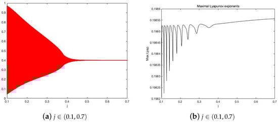
Figure 1. Bifurcation of System (8) in $(j,x)$–plane and maximal Lyapunov exponent.

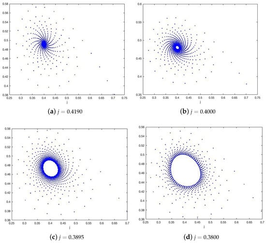
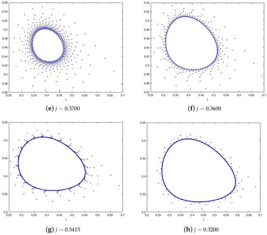
Figure 2. Phase portraits of System (8) with $f=0.2$, $g=0.1$ and $h=0.1$ and different j when the initial value $(x_0,y_0)=(0.4,0.2).$

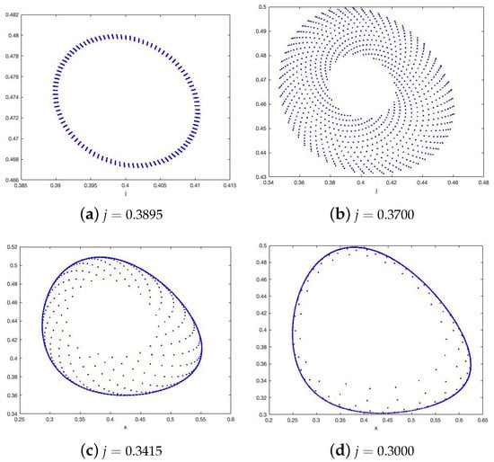
Figure 3. Phase portraits for System (8) with $f=0.2$, $g=0.1$ and $h=0.1$ and different j when the initial value $(x_0,y_0)=(0.4,0.48).$

Figure 1a shows the bifurcation diagram of System (8) on the $(j,x)$-plane, from which the fixed point $P_3=(0.4000,0.47373)$ is stable when $j>j_0=0.3895$ while unstable when $j<j_0$. Hence, a Neimark–Sacker bifurcation occurs at the fixed point $P_3$ when $j=j_0$, whose multipliers are ${\lambda }_{1,2}=0.9520\pm 0.3061i$ with $|{\lambda }_{1,2}|=1$. The corresponding maximum Lyapunov exponent diagram of System (8) is plotted in Figure 1b, from which we can easily see that the maximal Lyapunov exponents are always positive when the parameter $j\in (0.1,0.7)$. That is to say, at this time, chaos occurs. This is a kind of new phenomenon whose continuous system does not exist.

Figure 2a–h and Figure 3a–d show that the dynamical properties of the fixed point $P_3$ change from stable to unstable as the value of the parameter j decreases and there is an occurrence of invariant closed curve around $P_3$ when $j=j_0$, which agrees with the result of Theorem 6.

From the phase portraits in Figure 2 and Figure 3, we infer the stability of $P_3$. Figure 2e–h show that the closed curve is stable outside, while Figure 3a–d indicate that the closed curve is stable inside for the fixed point $P_3$ as long as the assumptions of Theorem 6 hold.

5. Conclusions

In this paper, we mainly give a detailed analysis of the bifurcations of System (8), which is the discrete version of a modified Leslie– Gower model with harvesting and alternative food for predator and Holling-II functional response [1]. We first derive that System (8) has four non-negative fixed points $P_0=(0,0),P_1=(0,Y_1),P_2=(1,0)$ and $P_3=(\frac{g-fh}{f},(1-\frac{g-fh}{f})(\frac{g-fh}{f}+j))$, and obtain the stability of the fixed points by using Definition 1 and Lemma 1. Then, we obtain the sufficient conditions for the occurrences of the transcritical bifurcation at the fixed point $P_2$ and Neimark–Sacker bifurcation at the fixed point $P_3$ by using the Center Manifold Theorem and bifurcation theory. Finally, we present numerical simulations to confirm corresponding theoretical results and reveal new dynamics of System (8), where chaos may appear. This is also the biggest difference between the continuous system and its corresponding discrete version.

References

- García, C.C. Bifurcations on a discontinuous Leslie–Gower model with harvesting and alternative food for predators and Holling II functional response. Commun. Nonliner Sci. Numer Simul. 2023, 116, 106800. [Google Scholar] [CrossRef]
- Kuznetsov, Y.A.; Kuznetsov, I.A.; Kuznetsov, Y. Elements of Applied Bifurcation Theory; Springer: Berlin/Heidelberg, Germany, 1998; p. 112. [Google Scholar]
- Cai, Y.L.; Gui, Z.J.; Zhang, X.B.; Shi, H.B.; Wang, W.M. Bifurcations and pattern formation in a predator-prey model. Int. J. Bifurc. Chaos 2018, 28, 1850140. [Google Scholar] [CrossRef]
- Guan, X.N.; Wang, W.M.; Cai, Y.L. Spatiotemporal dynamics of a Leslie–Gower predator-prey model incorporating a prey refuge. Nonlinear Anal. Real World Appl. 2011, 12, 2385–2395. [Google Scholar] [CrossRef]
- Luo, Y.T.; Zhang, L.; Teng, Z.D.; DeAngelis, D.L. A parasitism-mutualism-predation model consisting of crows, cuckoos and cats with stage-structure and maturation delays on crows and cuckoos. J. Theor. Biol. 2018, 446, 212–228. [Google Scholar] [CrossRef] [PubMed]
- Zhang, G.; Luo, Y.T.; Zhang, L.; Teng, Z.D.; Zheng, T.T. Coexistence for an almost periodic predator-prey model with intermittent predation driven by discontinuous prey dispersal. Discrete Dyn. Nat. Soc. 2017, 2017, 7037245. [Google Scholar]
- Wang, J.; Cai, Y.L.; Fu, S.M.; Wang, W.M. The effect of the fear factor on the dynamics of a predator-prey model incorporating the prey refuge. Chaos 2019, 29, 083109. [Google Scholar] [CrossRef] [PubMed]
- Zhang, H.S.; Cai, Y.L.; Fu, S.M.; Wang, W.M. Impact of the fear effect in a prey-predator model incorporating a prey refuge. Appl. Math. Comput. 2019, 356, 328–337. [Google Scholar]
- Xiang, C.; Huang, J.C.; Wang, H. Linking bifurcation analysis of Holling–Tanner model with generalist predator to a changing environment. Stud. Appl. Math. 2022, 149, 124–163. [Google Scholar] [CrossRef]
- Leslie, P.H. Some further notes on the use of matrices in population mathematics. Biometrika 1948, 35, 213–245. [Google Scholar] [CrossRef]
- Nindjin, A.F.; Aziz-Alaoui, M.A.; Cadivel, M. Analysis of a predator–prey model with modified Leslie–Gower and Holling-type II schemes with time delay. Nonlinear Anal. Real World Appl. 2006, 7, 1104–1118. [Google Scholar]
- González-Olivares, E.; Mena-Lorca, J. A Rojas-Palma and JD. Flores, Dynamical complexities in the Leslie–Gower predator–prey model as consequences of the Allee effect on prey. Appl. Math. Model. 2011, 35, 366–381. [Google Scholar] [CrossRef]
- Zhang, N.; Chen, F.G.; Su, Q.Q.; Wu, T. Dynamic behaviors of a harvesting Leslie-Gower predator-prey model. Discrete Dyn. Nat. Soc. 2011, 2011, 473949. [Google Scholar] [CrossRef]
- Yue, Q. Dynamics of a Modified Leslie–Gower Predator–Prey Model with Holling-Type II Schemes and a Prey Refuge; SpringerPlus: Berlin/Heidelberg, Germany, 2016; Volume 5, p. 461. [Google Scholar]
- Ávila-Vales, E.; Estrella-González, Á.; Esquivel, E.R. Bifurcations of a Leslie-Gower predator prey model with Holling type III functional response and Michaelis-Menten prey harvesting. arXiv 2017, arXiv:1711.08081. [Google Scholar]
- Ruiz, P.C.T.; Berrío, L.M.G.; González, E. Una clase de modelo de depredación del tipo Leslie-Gower con respuesta funcional racional no monotónica y alimento alternativo para los depredadores. Sel MatemáTicas 2019, 6, 204–216. [Google Scholar] [CrossRef]
- Arancibia-Ibarra, C.; Flores, J. Dynamics of a Leslie–Gower predator–prey model with Holling type II functional response, Allee effect and a generalist predator. Math. Comput. Simul. 2021, 188, 1–22. [Google Scholar]
- Lin, Q.F.; Liu, C.L.; Xie, X.D.; Xue, Y.L. Global attractivity of Leslie–Gower predator-prey model incorporating prey cannibalism. Adv. Differ. Equ. 2020, 2020, 153. [Google Scholar] [CrossRef]
- Liu, Y.Q.; Li, X.Y. Transcritical bifurcation and flip bifurcation of a new discrete ratio-dependent predator-prey system. Qual. Theory Dyn. Syst. 2022, 21, 122. [Google Scholar]
- Ba, Z.; Li, X.Y. Period-doubling bifurcation and Neimark-Sacker bifurcation of a discrete predator-prey model with Allee effect and cannibalism. Electr. Res. Arch. 2023, 31, 1406–1438. [Google Scholar]
- Xia, S.S.; Li, X.Y. Complicate dynamics of a discrete predator-prey model with double Allee effect. Math. Model. Control 2022, 2, 282–295. [Google Scholar] [CrossRef]
- Yao, W.B.; Li, X.Y. Complicate bifurcation behaviors of a discrete predator–prey model with group defense and nonlinear harvesting in prey. Appl. Anal. 2023, 102, 2567–2582. [Google Scholar] [CrossRef]
- Dong, J.G.; Li, X.Y. Bifurcation of a discrete predator-prey model with increasing functional response and constant-yield prey harvesting. Electr. Res. Arch. 2022, 30, 3930–3948. [Google Scholar] [CrossRef]
- Pan, Z.K.; Li, X.Y. Stability and Neimark–Sacker bifurcation for a discrete Nicholson’s blowflies model with proportional delay. J. Differ. Equat. Appl. 2021, 27, 250–260. [Google Scholar] [CrossRef]
- Din, Q. Complexity and chaos control in a discrete-time prey-predator model. Commun. Nonliner Sci. Numer. Simul. 2017, 49, 113–134. [Google Scholar] [CrossRef]
- Hu, Z.Y.; Teng, Z.D.; Zhang, L. Stability and bifurcation analysis of a discrete predator-prey model with nonmonotonic functional response. Nonlinear Anal. Real World Appl. 2011, 12, 2356–2377. [Google Scholar] [CrossRef]
- Li, W.; Li, X.Y. Neimark-Sacker bifurcation of a semi-discrete hematopoiesis model. J. Appl. Anal. Comput. 2018, 8, 1679–1693. [Google Scholar]
- Wang, C.; Li, X.Y. Further investigations into the stability and bifurcation of a discrete predator-prey model. J. Math. Anal. Appl. 2015, 422, 920–939. [Google Scholar] [CrossRef]
- Wang, C.; Li, X.Y. Stability and Neimark-Sacker bifurcation of a semi-discrete population model. J. Appl. Anal. Comput. 2014, 4, 419–435. [Google Scholar]
- Berezansky, L.; Braverman, E.; Idels, L. Mackey-Glass model of hematopoiesis with non-monotone feedback: Stability, oscillation and control. Appl. Math. Comput. 2013, 219, 6268–6283. [Google Scholar] [CrossRef]
- Gallay, T. A center-stable manifold theorem for differential equations in Banach spaces. Commun. Math. Phys. 1993, 152, 249–268. [Google Scholar] [CrossRef]
- Jorba, A.; Masdemont, J. Dynamics in the center manifold of the collinear points of the restricted three body problem. Phys. D. 1999, 132, 189–213. [Google Scholar] [CrossRef]
- Knobloch, E.; Wiesenfeld, K.A. Bifurcations in fluctuating systems: The center-manifold approach. J. Stat. Phys. 1983, 33, 611–637. [Google Scholar] [CrossRef]
- Xin, B.G.; Wu, Z.H. Neimark-Sacker bifurcation analysis and 0-1 chaos test of an interactions model between industrial production and environmental quality in a closed area. Sustainability 2015, 7, 10191–10209. [Google Scholar] [CrossRef]
- Winggins, S.; Golubitsky, M. Introduction to Applied Nonlinear Dynamical Systems and Chaos; Springer: Berlin/Heidelberg, Germany, 2003; Volume 2. [Google Scholar]
Disclaimer/Publisher’s Note: The statements, opinions and data contained in all publications are solely those of the individual author(s) and contributor(s) and not of MDPI and/or the editor(s). MDPI and/or the editor(s) disclaim responsibility for any injury to people or property resulting from any ideas, methods, instructions or products referred to in the content. |
© 2023 by the authors. Licensee MDPI, Basel, Switzerland. This article is an open access article distributed under the terms and conditions of the Creative Commons Attribution (CC BY) license (https://creativecommons.org/licenses/by/4.0/).