The Fama–French Five-Factor Model with Hurst Exponents Compared with Machine Learning Methods

Abstract

Scholars and investors have been interested in factor models for a long time. This paper builds models using the monthly data of the A-share market. We construct a seven-factor model by adding the Hurst exponent factor and the momentum factor to a Fama–French five-factor model and find that there is a 7% improvement in the average R–squared. Then, we compare five machine learning algorithms with ordinary least squares (OLS) in one representative stock and all A-Share stocks. We find that regularization algorithms, such as lasso and ridge, have worse performance than OLS. SVM and random forests have a good improvement in fitting power, while the neural network is not always better than OLS, depending on the data, frequency, period, etc.

1. Introduction

Factor models are always a point of interest in the field of quantitative investment. In 2015, Fama and French extended the well-known three-factor model by adding a profit factor (RMW) and investment factor (CMA), which resulted in a five-factor model. Since then, the five-factor model has attracted more and more attention in both theoretical and empirical aspects. However, in recent years, the research on factors is not limited to the five-factor model, as more possible factors have been discovered, such as the momentum factor and the memory factor, which are described using the Hurst parameter. The celebrated works of Carhart [1], Jegadeesh, and Titman [2] encourage the industry to find more and more new factors.

Many researchers have been interested in the momentum factor and memory effect in recent years. For example, Jegadeesh and Titman [2] found the momentum effect first, and Carhart [1] figured out the different maturities of the momentum effect and invented the momentum factor. Another famous factor is the Hurst exponent. Hurst [3] initially invented a method called the rescaled range analysis to estimate the Hurst exponent. Mandelbrot [4] used this method for the future market and found that the future price of cotton presented the nature described by the Hurst exponent. From then on, there has been a lot of literature published that is interested in estimating the Hurst exponent. Robinson [5] proposed the local Whittle estimator for the Hurst index and stated that the local Whittle estimation is better than the log–periodogram estimator of Geweke and Porter-Hudak [6]. Peng et al. [7], based on the DNA mechanism, invented detrended fluctuation analysis. In fact, some researchers study the momentum factor and the memory fact in the factor model paradigm. For example, Li et al. [8] considered the effectiveness of the momentum factor and the memory factor. This paper aims to achieve something deeper than just verifying factors.

To be specific, we carried out research to compare machine learning algorithms and the classical factor model based on OLS. Traditional models, which often rely on linear regression, break down when the explanatory variables are strongly correlated. Fortunately, as stated by Christensen et al. [9], this weakness can be covered by machine learning algorithms. A lot of work has been carried out, for example, Caporin and Poli [10] investigate lasso, Rahimikia and Poon [11] explore neural networks, and Luong and Dokuchaev [12] use random forests.

The contributions of this study have five aspects. First, this paper introduces the Hurst exponent as a factor and compares two different algorithms, finding that different algorithms do not differ. Second, this paper introduces the momentum factor and the Hurst exponent into factor models; they are both memory factors, but they are complementary rather than replaceable. Third, with a longer period, the Hurst exponent is stable, while the momentum factor is stronger in a shorter period. Fourth, this study proposes different machine learning algorithms and finds that SVM and random forest are better than OLS. The neural network is worse than OLS in small datasets. Lasso and ridge are worse than OLS, and this result verifies the usefulness of the seven factors.

Our paper is arranged as follows: Section 2 introduces the factor model proposed by Fama and French [13] and explains two algorithms for the Hurst exponent and momentum factor. Moreover, this section introduces four types of machine learning algorithms, which are regularization algorithms, SVM, neural networks, and random forests. Section 3 conducts empirical research on a five-factor model and a seven-factor model and checks the robustness of the results. Then, we make a comparison between four machine learning algorithms and a classic seven-factor model based on OLS. Section 4 states the contributions and conclusions.

2. Models

2.1. Five-Factor Model

The capital asset pricing model, which is a benchmark model describing stock returns as a risk-free rate plus market premium risk return, can be described as follows:

$$R_{\mathrm{it}}-R_{\mathrm{ft}}=a_i+b_i\left(Mk{t}_t-R_{\mathrm{ft}}\right)+e_{it},$$

(1)

where $R_{\mathrm{it}}$ is the return on stock i at period t, $R_{\mathrm{ft}}$ is the risk-free return, and $Mk{t}_t$ is the return on market index.

Fama and French [13] extended (1) by introducing two new factors. Thus, a new three-factor model is proposed:

$$R_{\mathrm{it}}-R_{\mathrm{ft}}=a_i+b_{i}Mk{t}_t+s_{i}SM{B}_t+h_{i}HM{L}_t+e_{it}$$

(2)

where $SM{B}_t$ is the difference between returns on a portfolio of stocks with small market value and stocks with big market value. $HM{L}_t$ is the difference between the returns on portfolios of high book-to-price value and low book-to-price value stocks.

Recently, by adding the profitability and investment factors to the three-factor model of Fama and French [13], they introduce a new five-factor asset pricing model:

$$R_{\mathrm{it}}-R_{\mathrm{ft}}=a_i+b_{i}Mk{t}_t+s_{i}SM{B}_t+h_{i}HM{L}_t+r_{i}RM{W}_t+c_{i}CM{A}_t+e_{it}$$

(3)

where $RM{W}_t$ is the returns of portfolios with robust profitability minuses with the returns of portfolios with weak profitability, $CM{A}_t$ is the returns of portfolios with low investment ability minus that with high investment ability, and $e_{it}$ is a zero-mean residual.

2.2. Hurst Exponent and Momentum Factor

The Hurst exponent describes the long-term memory of the price series, and the momentum factor describes the short-term memory of the price series. These two factors depict different aspects of the price series and may have additional information gain for the factor model. In this paper, we introduce two estimators of Berzin et al. [14], which have asymptotic properties, including consistency and asymptotic normality. Moreover, a momentum factor is also proposed.

2.2.1. Two Estimators of Hurst Exponents

Method 1:

$$\begin{array}{l}{r}_1=1\\ r_2=2\\ n_1=r_1\times floor(\frac{n}{2})\\ n_2=r_2\times floor(\frac{n}{2})\end{array}$$

where $n$ is sample size of $X_t$, and the floor function is a downward rounding function.

$$\begin{array}{l}{y}_1=\log \left(r_1\right)-0.5\left(\log \left(r_1\right)+\log \left(r_2\right)\right)\\ y_2=\log \left(r_2\right)-0.5\left(\log \left(r_1\right)+\log \left(r_2\right)\right)\end{array}$$

$$\begin{array}{l}{z}_1=\frac{y_1}{y_1^2+y_2^2}\\ z_2=\frac{y_2}{y_1^2+y_2^2}\end{array}$$

$z_1$ and $z_2$ calculated in this step are normalization coefficients.

$$\begin{array}{l}{M}_{n_1}={\displaystyle \sum _{k=1}^{n_1-2}\frac{1}{\left(n_1-1\right){\left(X_{2(k+2)}-2X_{2(k+1)}+X_{2k}\right)}^2}}\\ M_{n_2}={\displaystyle \sum _{k=1}^{n_2-2}\frac{1}{\left(n_2-1\right){\left(X_{k+2}-2X_{k+1}+X_k\right)}^2}}\end{array}$$

where $X_t$ are time series.

Finally, the calculation formula of the Hurst exponent is obtained:

$${\widehat{H}}_k=-0.5\left(z_1\log \left(M_{n_1}\right)+z_2\log \left(M_{n_2}\right)\right)$$

Method 2:

$$\begin{array}{l}{r}_1=1\\ r_2=2\\ n_1=r_1\times floor(\frac{n}{2})\\ n_2=r_2\times floor(\frac{n}{2})\end{array}$$

where $n$ is sample size of $X_t$, and the floor function is a downward rounding function.

$$\begin{array}{l}{y}_1=\log \left(r_1\right)-0.5\left(\log \left(r_1\right)+\log \left(r_2\right)\right)\\ y_2=\log \left(r_2\right)-0.5\left(\log \left(r_1\right)+\log \left(r_2\right)\right)\end{array}$$

$$\begin{array}{l}{z}_1=\frac{y_1}{y_1^2+y_2^2}\\ z_2=\frac{y_2}{y_1^2+y_2^2}\end{array}$$

$z_1$ and $z_2$ calculated in this step are normalization coefficients.

$$\begin{array}{l}{L}_{n_1}={\displaystyle \sum _{k=1}^{n_1-2}\frac{1}{\left(n_1-1\right)\left|X_{2(k+2)}-2X_{2(k+1)}+X_{2k}\right|}}\\ L_{n_2}={\displaystyle \sum _{k=1}^{n_2-2}\frac{1}{\left(n_2-1\right)\left|X_{k+2}-2X_{k+1}+X_k\right|}}\end{array}$$

The Hurst exponent is calculated using:

$${\widehat{H}}_{\log }=-0.5\left(z_1\log \left(L_{n_1}\right)+z_2\log \left(L_{n_2}\right)\right)$$

2.2.2. Momentum Factor

The momentum factor is defined as return of stocks for a given period:

$$MOM=\log (\frac{X_{i+k}}{X_i}),i=1,2,3,\dots n-k$$

where $X$ is the time series of stock price, and $k$ is the momentum factor parameter, usually 12 months (one year). In the following experiment, we adjusted the parameter of the momentum factor together with that of the Hurst exponents.

2.3. Machine Learning Methods

2.3.1. Support Vector Machine

SVM is a kind of supervised learning algorithm used to solve classification problems using a generalized linear classifier with the kernel function. SVM is developed from generalized portrait algorithm from the earliest work of Vladimir Vapnik [15]. With a series of developments, Cortes and Vapnik [16] invented a nonlinear SVM with soft margins and tested the algorithms of the handwritten character recognition problem.

2.3.2. Random Forests

Random forests were developed by Tin Kam Ho [17], who combined bootstrap aggregating with a random subspace method and created a gathering of decision trees. The final classification result is voted by all decision trees in the forest.

2.3.3. Forward Neural Network

Forward neural network is a kind of multilayer perception, which has a long history starting from the 1940s. Forward neural network usually consists of one input layer, several hidden layers, and one output layer. Between two layers, there is often an activation function, which is used to transfer the results from the last layer. The output layer gives the classification result or regression result.

2.3.4. Least Squares, Ridge Regression, Lasso

The OLS method was used as a benchmark in our research. For verification, we also tested the ridge regression, which incorporates the L2 regularization, and lasso, which incorporates the L1 regularization. These algorithms are all linear methods with different constraints.

3. Empirical Results

3.1. Five-Factor Model in A-Share Stock Market of China

In this subsection, the explanatory power of the Fama–French five-factor model in the A-share stock market (companies based in mainland China that are listed on either the Shanghai or Shenzhen stock exchanges) will be discussed. We will also analyze the performance of the Hurst factor and the MOM factor in the new factor model. The stock data used in this study are daily data from January 2010 to July 2020 driven from the Wind database. In the Wind database, it is the default setting that the monthly data of the time period is the closing price on the last day of each month. The financial data used in this section come from the quarterly financial reports of listed companies. There are always differences in the financial data collected at the end of each month in the A-share market, as listed companies announce their financial reports at different times. Both the Hurst exponent and the momentum factor were calculated based on the monthly stock price data.

Borrowing the idea of Fama and French [13], the four factors of SMB, HML, RMW, and CMA in the five-factor model were calculated based on the grouping of financial data on the monthly return rate of stocks. We calculated five factors based on the monthly stock price data from February 2010 to June 2020.

In the next step, we conducted an experiment to test the effectiveness of the five factors. This experiment built up a series of regression models, which consisted of $C_5^1+C_5^2+C_5^3+C_5^4+C_5^5$ kinds of different five-factor combinations. We evaluated these models using the Akaike information criterion (AIC) and selected the best model. At the same time, we calculated the proportions of five factors in all factor models, which were based on all A-share stocks (one stock has $C_5^1+C_5^2+C_5^3+C_5^4+C_5^5$ factor models, and we chose the best using the AIC and observed the distributions of five factors by calculating the proportions).

Table 1 summarizes the result of this experiment; among the $C_5^1+C_5^2+C_5^3+C_5^4+C_5^5$ regression models, the average R–squared is 40%. The most popular factor is MKT (with a proportion of 91%), RMW has a proportion of 51%, which ranks No. 2, SMB is 47%, HML is 38%, and CMA takes the last position.

Table 1. The proportion of the five factors in models selected using AIC of each stock.

Factor	MKT	SMB	HML	RMW	CMA
The proportion	0.91	0.47	0.38	0.51	0.042

3.2. The Factor Model with Hurst Exponent and Momentum Factor

The effectiveness of the Fama–French five-factor model, Hurst exponent, and momentum factor was investigated in the previous work of Li et al. [8]. As the different values of the Hurst exponent do not differ much (see the previous work by Li et al. [8]), we used ${\widehat{H}}_k$ to build up a seven-factor model. In this subsection, we aim to build up a benchmark, which is a traditional factor model based on OLS, and consider the change by adding the Hurst exponent and the momentum factor.

For the parameter and data setup, the longer parameters are more stable, so we used 36 months as the parameter of Hurst exponent and momentum factor. For robustness, we chose monthly price data longer than 70, which means the stocks were listed for more than 106 months (about 9 years); overall, there were 2249 stocks that met our setting.

The five-factor model based on OLS was our starting point. Figure 1 shows the root-mean-square deviation (RMSE) and R–squared distribution for OLS with a five-factor model of A-share stocks in China. The mean and standard deviation of RMSE are 0.0952 and 0.0221, respectively. The mean and standard deviation of R–squared are 0.4007 and 0.1128, respectively.

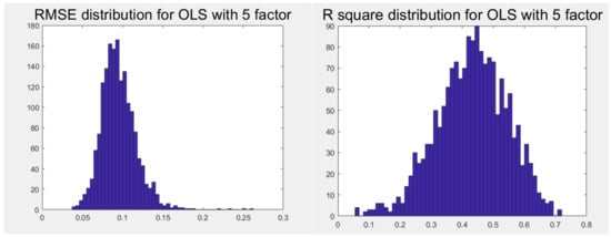
Figure 1. RMSE and R–squared distribution for 5-factor OLS of A-share stocks.

Next, two new factors, the Hurst exponent and the momentum factor, were added to the classic five-factor model. The length of the time series was needed to obtain both the Hurst exponent and the momentum factor. In this study, a length of 12 months was used for the preliminary study. Then, the values of the parameters were changed accordingly.

The momentum factor and the Hurst exponent were calculated using the ${\widehat{H}}_k$ algorithm, and the ${\widehat{H}}_{\log }$ algorithm was substituted into the five-factor model to build up a seven-factor model. As the different values of the Hurst exponent do not differ much (see the previous work by Li et al. [8]), we used $H_k$ to build up a seven-factor model at this stage.

Seven-factor models provide a better service than five-factor models; we can conclude this from the performance of the mean of R–squared, which is 0.4731 for ${\widehat{H}}_k$ and 0.4729 for ${\widehat{H}}_{\log }$ in the seven-factor models. Compared with the mean of R–squared in the five-factor models, whose value is only 0.4007, so the seven-factor models increase by 7% relative to the five-factor models from best models (by AIC) of $C_7^1+C_7^2+C_7^3+C_7^4+C_7^5+C_7^6+C_7^7$ kinds of models from an average perspective.

Table 2 presents the proportions of seven factors in $C_7^1+C_7^2+C_7^3+C_7^4+C_7^5+C_7^6+C_7^7$ kinds of seven-factor models. In the seven-factor models, MKT is still the most effective factor, MOM ranks second taking a proportion of 88%, and HML, SMB, and RMW perform as well as in the five-factor models. The Hurst exponent accounts for 22% for ${\widehat{H}}_k$ and 24% for ${\widehat{H}}_{\log }$. From this result, we see that different Hurst exponents do not differ much.

Table 2. The proportion of the 7 factors in model selected using AIC.

Factor	MKT	SMB	HML	RMW	CMA	MOM	Hurst
${\widehat{H}}_k$	0.94	0.49	0.33	0.51	0.046	0.88	0.22
${\widehat{H}}_{\log }$	0.94	0.48	0.33	0.51	0.046	0.88	0.24

To sum up, the Hurst exponent and MOM have a high proportion in seven-factor models; this result verifies the effectiveness of the seven-factor models. The more interesting thing is the relationship between the Hurst exponent and MOM.

Table 3 shows the answer to our question. There is only 9% of the seven-factor models that do not have either the Hurst exponent or MOM; this result emphasizes the importance of the Hurst exponent and MOM. Moreover, the “H and MOM” accounts for the models that have both the Hurst exponent and MOM; this proportion is around 20%. As 20% is a relatively high proportion, the Hurst exponent and MOM have a complementary relationship rather than a substitutional relationship.

Table 3. Proportion of models with different combinations of Hurst exponent and MOM.

Factor	None	H But no MOM	MOM But no H	H and MOM
${\widehat{H}}_k$	0.090475	0.030346	0.670413	0.208767
${\widehat{H}}_{\log }$	0.094409	0.028941	0.684743	0.191908

To compare with the machine learning experiments, we set up a benchmark using the OLS model. Figure 2 shows the distribution of RMSE and R–squared. The seven-factor models based on OLS achieve a mean RMSE as low as 0.097 and a mean R–squared of around 0.47.

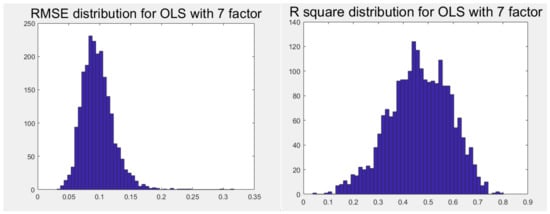
Figure 2. RMSE and R–squared distribution for seven-factor OLS of A-share stocks.

3.3. Portfolio Factor Analysis Based on OLS

For the robustness of the experiment, we built 10,000 random portfolios to repeat the seven-factor experiment. In total, 10,000 random portfolios consisted of 10 randomly selected stocks, and then, we obtained Table 4. Table 4 is consistent with Section 3.2.

Table 4. Proportion of each factor in 10,000 random portfolios of 10 stocks.

Factor	MKT	SMB	HML	RMW	CMA	MOM	Hurst
${\widehat{H}}_k$	0.97	0.55	0.33	0.53	0.052	0.35	0.28
${\widehat{H}}_{\log }$	0.97	0.55	0.32	0.52	0.052	0.36	0.27

The experiment on 10,000 random portfolios of 10 stocks achieves an R–squared of around 0.78, which is a better performance than that of Section 3.2. Additionally, the proportions of all factors are higher than that of the single-stock experiment. This result may profit from the diversity of portfolios.

Similarly, the result of 10,000 random portfolios of 30 stocks is given in Table 5. The average R–squared increases again and obtains a value as high as about 0.9; this result verifies the conclusion of Section 3.2.

Table 5. Proportion of each factor in 10,000 random portfolios of 30 stocks.

Factor	MKT	SMB	HML	RMW	CMA	MOM	Hurst
${\widehat{H}}_k$	0.990253	0.50288	0.393886	0.682322	0.100576	0.473638	0.40895
${\widehat{H}}_{\log }$	0.99359	0.516026	0.409341	0.689103	0.091117	0.462454	0.391026

3.4. Robustness Test

Next, we changed the values of the momentum factor and the Hurst exponent to make a systematic comparison. We also tested whether the term parameters of MOM and Hurst exponent changes have a significant impact on our results. The term parameters are 12 months, 24 months, and 36 months.

First, we checked the R–squared when we tuned the term parameters. The R–squared varies from 0.47 to 0.51, while the term parameter increases from 12 months to 36 months in Table 6. We can conclude that tuning the term parameter does not affect the explanatory power of the seven-factor models.

Table 6. Mean of R–squared by tuning term parameter with two kinds of Hurst exponents (both H and MOM).

Algorithm/Parameter	12 Months	24 Months	36 Months
${\widehat{H}}_k$	0.47	0.47	0.49
${\widehat{H}}_{\log }$	0.47	0.47	0.51

We checked the robustness of the seven factors using the tuning term parameters. The proportion of seven factors represents the effectiveness of the factors. From Table 7, MKT maintains a proportion of 93%, which ranks first. SMB, HML, and RMW have a stable performance when the term parameter changes from 12 months to 36 months; this result validates the previous literature. MOM’s proportion gradually decreases when the term parameter increases. A reasonable explanation for this is that the MOM factor captures the short-time trends, which contribute to the model’s explanatory power; if we raise the term parameter, the short-term effect will decrease. On the contrary, the Hurst exponent holds the proportion at around 22–29%, which exhibits the long-term properties of the Hurst exponent.

Table 7. The proportion of each factor by tuning term parameter (both H and MOM).

Panel A: Time Parameter Equals 12 Months
Algorithm/Factor	MKT	SMB	HML	RMW	CMA	MOM	Hurst
${\widehat{H}}_k$	0.94	0.48	0.33	0.51	0.05	0.88	0.24
${\widehat{H}}_{\log }$	0.94	0.49	0.33	0.51	0.05	0.88	0.22
Panel B: Time Parameter Equals 24 Months
Algorithm/Factor	MKT	SMB	HML	RMW	CMA	MOM	Hurst
${\widehat{H}}_k$	0.93	0.52	0.37	0.48	0.06	0.62	0.27
${\widehat{H}}_{\log }$	0.93	0.52	0.38	0.47	0.06	0.62	0.25
Panel C: Time Parameter Equals 36 Months
Algorithm/Factor	MKT	SMB	HML	RMW	CMA	MOM	Hurst
${\widehat{H}}_k$	0.94	0.54	0.40	0.49	0.09	0.52	0.27
${\widehat{H}}_{\log }$	0.92	0.53	0.41	0.49	0.09	0.53	0.29

Figure 3 and Figure 4 show the importance of the seven factors in terms of the Shapley value. The Shapley value has been revised by Giudici and Raffinetti [18]. This metric leads to a variable contribution measure that is more generally applicable and easier to interpret. The expression of the marginal contribution shows how global explanations can be mapped to local ones and vice versa. We used the Shapley value in this paper to compare the importance of factors. Figure 3 uses ${\widehat{H}}_k$ as the Hurst exponent, and Figure 3 uses ${\widehat{H}}_{\log }$ as the Hurst exponent. The results of the two figures are similar: the most important factor is MKT, and the second is RMW in Figure 3 and SMB in Figure 4. The rank of the seven factors is similar to that of Table 7.

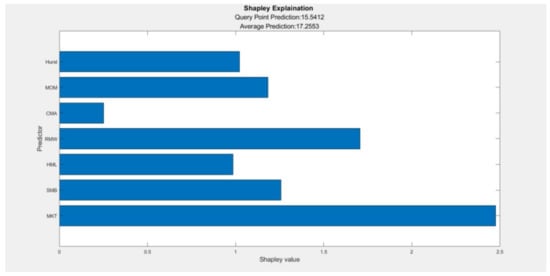
Figure 3. Shapley value of 7 factors (Hurst using ${\widehat{H}}_k$).

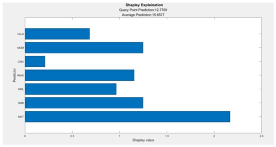
Figure 4. Shapley value of 7 factors (Hurst using ${\widehat{H}}_{\log }$).

3.5. One Stock Test with Machine Learning Method

We took 000001.XSHE, which is the Shanghai composite index, as an example to test the effects of different machine learning algorithms. In this subsection, we introduce four different type machine learning algorithms, which are regularization methods (lasso and ridge), SVM, forward network, and random forests, and use seven factors (apart from Fama–French five factors, we chose the Hurst exponent and the momentum factor with the 36-month parameter) as predictors to explain the return of 000001.XSHE. OLS obtains a result of RMSE of 0.0559 and 0.6334 of R–squared; we compared this result with four machine learning algorithms.

3.5.1. Lasso and Ridge

We used values of k from 0.01 to 10 and obtained the change trace of RMSE and R–squared.

Figure 5 shows RMSE changing with ridge parameter $\mathrm{k}$. The upward line indicates that RMSE rises with $\mathrm{k}$ becoming bigger. This result illustrates a small $\mathrm{k}$ when we used ridge.

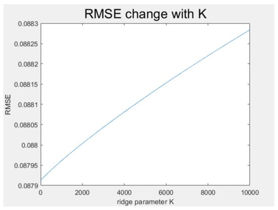
Figure 5. RMSE of ridge for 000001.XSHE.

Figure 6 shows the R–squared value changing with ridge parameter k in the downward line in line with the conclusion of Figure 5.

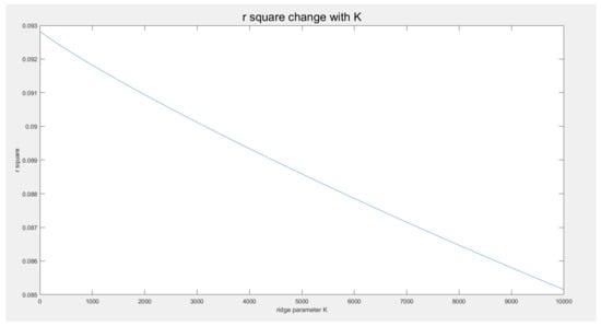
Figure 6. R–squared of ridge for 000001.XSHE.

The result of lasso is similar to ridge, which is shown in Figure 7. The RMSE decreases at first and then rises, which means that there are some redundant predictors, but mostly, the predictors are useful. Moreover, the R–squared line suggests the same. Therefore, to minimize the effect of shrinkage, we chose the smallest k and obtained the 4 evaluation indicators of these two models, as shown in Table 8.

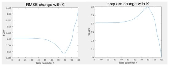
Figure 7. RMSE and R–squared of lasso for 000001.XSHE.

Table 8. 4 evaluation indicators of ridge and lasso.

000001.XSHE	Ridge	Lasso
RMSE	0.0879	0.0708
R–squared	0.0928	0.4116
NRMSE	0.9525	0.7671
MAE	0.0697	0.0614

As the seven factors are all useful to explain the return of stocks, any decrease in the factors is not suitable. Consequently, the R–squared of lasso and ridge decreases.

3.5.2. SVM

SVM can be used in regression problems. We used the seven factors as the independent variable and used the return of 000001.XSHE as the dependent variable.

Figure 8 shows the return and forecast return of 000001.XSHE. Although there is a forecast error in prediction, generally, the return trend was captured using SVM. The RMSE is 0.0602, and the R–squared is 0.5744. Compared with the result of OLS, SVM is a little inferior based on RMSE and R–squared. The main reason why SVM is inferior to OLS is that 000001.XSHE is a large-cap stock, which can be mainly explained by seven factors, and SVM is useful because it can use the kernel function to suggest nonlinear predictions, which is not significant in this case.

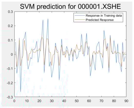
Figure 8. Return and forecast return of 000001.XSHE.

3.5.3. Forward Network

The forward network is a kind of neural network algorithm. Using the seven factors as predictors, we introduced two hidden layers, which had 10 and 5 neurons, respectively. The network structure is shown in Figure 9.

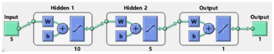
Figure 9. Forward network structure of two hidden layers.

This model achieves a result of 0.0549 in RMSE and 0.6466 in R–squared. This result is better than that of OLS because of the strong fitting capacity of the neural network.

3.5.4. Random Forests

Random Forests is a bagging of decision trees. The prediction error will be lower as the number of trees increases until the model is fully fitted. Figure 10 presents how the error decreases with the increase in the number of trees.

Figure 10. Error decreases with the increase in the number of trees.

We set two hundred trees and no more than five samples in one leaf as the parameters of this case. From Figure 10, we can see that the out-of-bag classification error decreases at first, but changes around 5.75 × 10⁻³ when the number of trees is more than 40. This result indicates that although random forests have good fitting capacity, there is a limit to minimizing error. The random forests obtained values of 0.0482 in RMSE and 0.7268 in R–squared, which beats all of the models in this case.

3.6. Research of Five Machine Learning

In this section, we use five machine learning algorithms to compare their explanatory power with that of the traditional OLS model on all of stocks in the A-share stock market. The seven-factor model based on ridge and lasso is a counterexample to the OLS model. As the factors are all useful, we assumed any shrinkage to factors will lower the efficiency of the model and chose a small parameter when using these two models.

Figure 11 shows the RMSE distribution of ridge and lasso. Both distributions have a mean bigger than OLS, and the positive tails are both very long, which indicates that ridge and lasso are not efficient in some stocks because of a big RMSE.

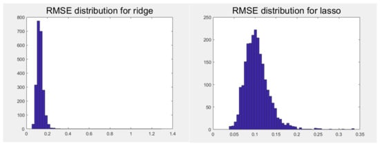
Figure 11. RMSE distribution for ridge and lasso of A-share stocks.

Table 9 gives the mean RMSE of ridge and lasso, which are 0.13 and 0.1049, respectively. Upon closer inspection, we recognize that both ridge and lasso perform worse than OLS, which has a mean RMSE of 0.0969. This result verifies the importance of factor. However, for the other time periods, data, or frequencies, we do not promise consistency.

Table 9. Mean and std. of RMSE of ridge and lasso.

RMSE	Ridge	Lasso
Mean	0.13	0.1049
Std.	0.0404	0.0298

The R–squared of ridge and lasso has the same result, which is shown in Figure 12. Ridge makes the R–squared value nearly zero; lasso does better than ridge but still worse than OLS. Both distributions have a long negative tail, which means many stocks cannot be explained using lasso and ridge. Figure 12 shows that ridge has an R–squared near to zero; lasso is a little better but worse than OLS.

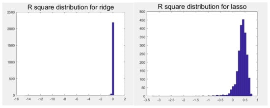
Figure 12. R–squared distribution for ridge and lasso of A-share stocks.

Table 10 presents the mean and standard deviation of the R–squared of lasso and ridge. The statistics in Table 9 enhance the conclusion that the seven factors are all useful, and shrinkage in the models is not appropriate.

Table 10. Mean and std. of R–squared of ridge and lasso.

R–Squared	Ridge	Lasso
Mean	0.0454	0.3619
Std.	0.3446	0.2352

Figure 13 illustrates the NRMSE distribution for ridge and lasso of A-share stocks. The NRMSE distribution of ridge is very narrow, while that of lasso is much wider. That is to say, the NRMSE of many stocks is stable in terms of ridge, while the NRMSE of stocks in terms of lasso is inconsistent.

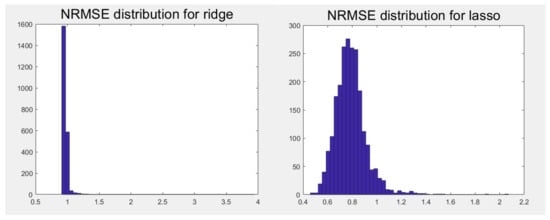
Figure 13. NRMSE distribution for ridge and lasso of A-share stocks.

Table 11 shows the mean and std. of NRMSE of ridge and lasso. The mean value of ridge is a little larger than that of lasso in terms of NRMSE. However, as the NRMSE is nearly one, both ridge and lasso do not perform well in terms of NRMSE.

Table 11. Mean and std. of NRMSE of ridge and lasso.

NRMSE	Ridge	Lasso
Mean	0.9733	0.7885
Std.	0.0850	0.1283

Figure 14 presents a similar result in terms of MAE; ridge is somewhat stable, while lasso is differential. Table 12 shows that the mean value of the MAE of ridge is a little larger than that of lasso.

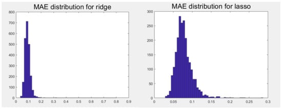
Figure 14. MAE distribution for ridge and lasso of A-share stocks.

Table 12. Mean and std. of MAE of ridge and lasso.

MAE	Ridge	Lasso
Mean	0.0919	0.0781
Std.	0.0262	0.0225

Figure 15 presents the RMSE distribution for SVM, neural network, and random forests of A-share stocks. Together with Table 13, we find that SVM and random forests have a lower RMSE than that of OLS, but the RMSE of the neural network is a little bit higher than OLS, which is contrary to our expectations. One reasonable explanation for this result is that the neural network has multiple layers and neurons, and weight updates come from error corrections, which rely on big data. In our research, we used the monthly data of A-share stocks, and the majority of stocks had less than 100 months of price points. That is why the neural network cannot show its explanatory power.

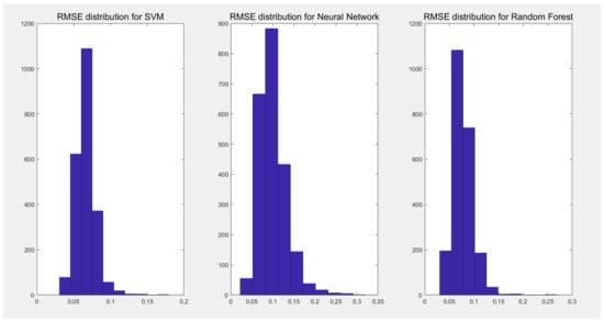
Figure 15. RMSE distribution for SVM, neural network, and random forests of A-share stocks.

Table 13. Mean and std. of RMSE, SVM, neural network, and random forests.

RMSE	SVM	NN	Random Forests
Mean	0.066782	0.100411	0.077410588
Std	0.013501	0.033212	0.020454047

The R–squared distribution for SVM, neural network, and random forests of A-share stocks in Figure 16 also suggest that SVM and random forests obtain a higher R–squared, and the neural network’s R–squared is a little lower. In particular, SVM beats all the other models with a mean R–squared as high as 0.717676, as shown in Table 14.

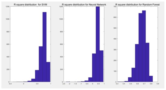
Figure 16. R–squared distribution for SVM, neural network, and random forests of A-share stocks.

Table 14. Mean and std. of R–squared of SVM, neural network, and random forests.

R–Squared	SVM	NN	Random Forests
Mean	0.717676	0.407488	0.660278594
Std	0.13547	0.271846	0.066090287

Figure 17 shows the NRMSE distributions of SVM, neural network, and random forests. The left tail of the NRMSE distributions of SVM obtains the lowest value among the three machine learning algorithms. Table 15 presents the mean NRMSE of SVM as 0.5171, which is also the lowest.

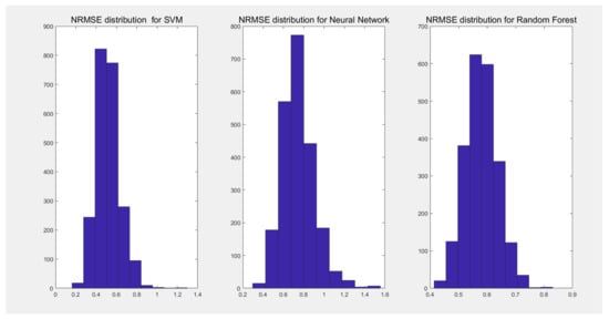
Figure 17. NRMSE distribution for SVM, neural network, and random forests of A-share stocks.

Table 15. Mean and std. of NRMSE of SVM, neural network, and random forests.

NRMSE	SVM	NN	Random Forests
Mean	0.5171	0.7467	0.5803
Std	0.1164	0.1598	0.0561

Figure 18 shows the MAE distributions of three machine learning algorithms. SVM still performs best among the three machine learning algorithms, and random forest ranks second because of its long right tail. Table 16 presents that the mean value of the MAE of SVM is 0.0494, which is the lowest, the random forest is 0.0514, and the neural network is 0.0711, and its std. is 0.0234, which means that both the mean value and std. of the MAE of the neural network are worse than SVM.

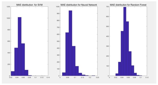
Figure 18. MAE distribution for SVM, neural network, and random forests of A-share stocks.

Table 16. Mean and std. of MAE of SVM, neural network, and random forests.

MAE	SVM	NN	Random Forests
Mean	0.0494	0.0711	0.0519
Std	0.0096	0.0234	0.0114

Conditional superior predictive ability (CSPA) was invented by Jia Li et al. [19]. This tool provides a function to compare the target model against one benchmark model under one conditional variable. CSPA is functional in nature. Under the null hypothesis, the benchmark’s conditional expected loss is no more than those of the competitors, uniformly across all conditioning states. This is the first application of conditional moment-inequality methods in time-series econometrics, and the theoretical tools developed here are broadly useful for other types of inference problems involving partial identification and dependent data. In this experiment, we took OLS as the benchmark and the return series of 000001.XSHE as the conditional variable.

Table 17 shows the theta_p value and the result of rejecting at a 10% confidence level for 000001.XSHE. The theta_p value is a statistic indicating the degree of conditional superior predictive ability. A negative theta_p value means that this target model beats the benchmark model and vice versa. The rejs value shows the result of rejecting at a 10% confidence level: a result of 1 indicates that the target model is better; otherwise, the benchmark model is better. The results in Table 17 suggest that random forest is the best model with the lowest theta_p value and that ridge is better than lasso, which gives a different result compared with previous research. Moreover, although ridge beats OLS, the theta_p value of ridge is nearly 0; that is to say, ridge may be not always better than OLS if we change datasets.

Table 17. Five machine learning algorithms vs. OLS in terms of CSPA for 000001.XSHE.

	Ridge	Lasso	SVM	NN	Random Forest
Theta_p	−0.00145	0.008906	−0.00374	−0.00223	−0.01543
Rejs	1	0	1	1	1

Next, we visualized the result of ridge and lasso vs. OLS in the return series with 000001.XSHE as the conditional variable. The X-axis shows the return series of 000001.XSHE from low to high; the red lines are ridge and lasso. When the red lines are lower than the confidence boundary (dash line), ridge and lasso are better than OLS, and vice versa. Figure 19 shows that lasso is worse than OLS when the return series of 000001.XSHE is in the middle, while ridge is always better in this experiment.

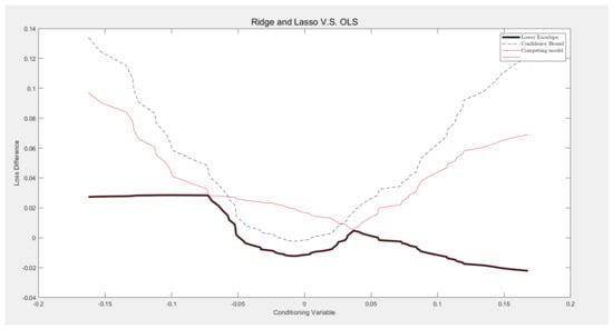
Figure 19. Ridge and lasso vs. OLS under return series with 000001.XSHE as conditional variable.

We also compared SVM, neural network, and random forest with OLS. We can see from Figure 20 that all three models are lower than the confidence boundary all the time. This result means SVM, neural network, and random forest beat OLS stably.

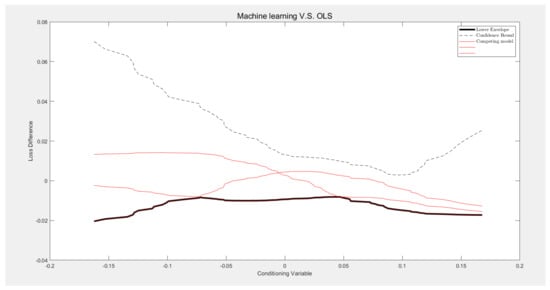
Figure 20. SVM, neural network, and random forest vs. OLS under return series with 000001.XSHE as conditional variable.

4. Discussion

This paper is a continuation of the previous work by Li et al. [8]. Research is always carried out to discover something in $X\stackrel{f}{\to }Y$. The previous work by Li et al. [8] researches the Fama–French five factors, Hurst exponents, and momentum factors, and so, the previous work focuses on $X$. This paper extends the seven-factor model by introducing machine learning algorithms, which is to say, we focus on $f$.

In the previous work by Li et al. [8], they only verify the effectiveness of factors and the relationship among factors. In this paper, we not only verify the effectiveness of machine learning methods but also discover the different performance of machine learning methods. For example, we found that some of the machine learning methods are better than OLS, such as SVM, neural network, and random forest. However, ridge and lasso do not always do better than OLS, especially in the given datasets in monthly frequency. While the CSPA test shows the significance of the model difference in another way in that SVM and random forest beat OLS significantly, but ridge and neural network are weaker, lasso is overall worse than OLS in the experiment for 000001.XSHE. This result may change with the data size, frequency, period, and factor effectiveness. Compared with Takaishi [20], our work introduced the momentum factor, which is a short-term factor and has complementary effects on the Hurst exponents. Moreover, we compared the two different Hurst exponents, which are ${\widehat{H}}_k$ and ${\widehat{H}}_{\log }$. We found that different algorithms of Hurst exponents do not have a significant difference in the performance of factor models.

5. Conclusions

This paper contributes to two aspects.

For the comparison of factors, we checked seven factors one by one. MKT is the most effective factor no matter how the term parameter changes. SMB, HML, and RMW are classic factors with a stable performance in five-factor models and seven-factor models. CMA is the weakest factor in all experiments. MOM ranks second in the seven-factor models when the term parameter is 12 months. However, with the increase in term parameters, the proportion of MOM factor in the seven-factor models decreases gradually, while the Hurst exponent remains stable when the term parameter is tuning. In addition to the result of the proportions, we also checked the Shapley value of seven factors. The result of the Shapley value does not differ much from that of the proportions. Therefore, we can conclude that the Hurst exponent and MOM represent the stock return rate in different term structures; the Hurst exponent shows the long-term factor, while MOM shows the effect in the short term.

For a comparison of the models, we used the AIC criterion to use the models in different factor combinations. We found that the seven-factor model has an average R–squared that is 7% higher than that of the five-factor models. Then, we set the OLS model as the baseline to compare the machine learning methods with OLS. From the conclusion of the previous work by Li et al. [8], we see that all factors are meaningful in explaining the return of stocks. Therefore, lasso and ridge were used to lower the fitting capacity of the model in this experiment, but the result may change using other data or other frequencies. We used RMSE, R–squared, NRMSE, and MAE as evaluations to compare the five machine learning algorithms. Generally speaking, lasso and ridge do not perform better than OLS. However, the CSPA test shows that sometimes ridge may perform better than OLS, while lasso may be worse than OLS in an experiment for 000001.XSHE. Of the other three machine learning algorithms, SVM (average R–squared is 0.717676) and random forests (average R–squared is 0.660278594) perform excellently, but the neural network (average R–squared is 0.407488) performance is a little worse than OLS due to the lack of the monthly data of stocks (although the CSPA test shows that the neural network beats OLS, but its theta_p is not negative enough). Therefore, we can see that machine learning is not always stronger than the classic OLS method, and the effectiveness of machine learning methods depends on the data size, frequency, period, and factor effectiveness.

References

- Carhart, M.M. On Persistence in Mutual Fund Performance. J. Financ. 1997, 52, 57–82. [Google Scholar] [CrossRef]
- Jegadeesh, N.; Titman, S. Returns to buying winners and selling losers: Implications for market efficiency. J. Financ. 1993, 48, 65–91. [Google Scholar] [CrossRef]
- Hurst, H.E. Long-term storage capacity of reservoirs. Trans. Am. Soc. Civ. Eng. 1951, 116, 770–808. [Google Scholar] [CrossRef]
- Mandelbrot, B. The variation of certain speculative prices. J. Bus. 1963, 36, 394–419. [Google Scholar] [CrossRef]
- Robinson, P.M. Gaussian Semiparametric Estimation of Long Range Dependence. Ann. Stats 1995, 23, 1630–1661. [Google Scholar] [CrossRef]
- Geweke, J.; Porter-Hudak, S. The estimation and application of long memory time series models. J. Time Ser. Anal. 1983, 4, 221–238. [Google Scholar] [CrossRef]
- Peng, C.K.; Buldyrev, S.V.; Havlin, S. Mosaic organization of DNA nucleotides. Phys. Rev. E 1994, 49, 1685–1689. [Google Scholar] [CrossRef] [PubMed]
- Li, Y.; Teng, Y.; Shi, W.; Sun, L. Is the Long Memory Factor Important for Extending the Fama and French five-facor Model: Evidence from China. Math. Probl. Eng. 2021, 2021, 2133255. [Google Scholar]
- Christensen, K.; Siggaard, M.; Veliyev, B. A machine learning approach to volatility forecasting. SSRN 2021, nbac020. [Google Scholar] [CrossRef]
- Caporin, M.; Poli, F. Building news measures from textual data and an application to volatility forecasting. Econometrics 2017, 5, 35. [Google Scholar] [CrossRef]
- Rahimikia, E.; Poon, S.-H. Machine Learning for Realised Volatility Forecasting. SSRN 2020. [Google Scholar] [CrossRef]
- Luong, C.; Dokuchaev, N. Forecasting of realised volatility with the random forests algorithm. J. Risk Financ. Manag. 2018, 11, 61. [Google Scholar] [CrossRef]
- Fama, E.F.; French, K.R. A five-factor asset pricing model. J. Financ. Econ. 2015, 116, 1–22. [Google Scholar] [CrossRef]
- Berzin, C.; Latour, A.; Leon, J.R. Inference on the Hurst Parameter and the Variance of Diffusions Driven by Fractional Brownian Motion; Springer: Berlin/Heidelberg, Germany, 2014; Volume 216. [Google Scholar]
- Vapnik, V. Pattern recognition using generalized portrait method. Autom. Remote Control 1963, 24, 774–780. [Google Scholar]
- Cortes, C.; Vapnik, V. Support-vector networks. Mach. Learn. 1995, 20, 273–297. [Google Scholar] [CrossRef]
- Ho, T.K. Random decision forests. In Proceedings of the IEEE 3rd International Conference on Document Analysis and Recognition, Montreal, QC, Canada, 14–16 August 1995; Volume 1, pp. 278–282. [Google Scholar]
- Giudici, P.; Raffinetti, E. Shapley-Lorenz eXplainable artificial intelligence. Expert Syst. Appl. 2021, 167, 114104. [Google Scholar] [CrossRef]
- Li, J.; Liao, Z.; Quaedvlieg, R. Conditional superior predictive ability. Rev. Econ. Stud. 2022, 89, 843–875. [Google Scholar] [CrossRef]
- Takaishi, T. Rough volatility of Bitcoin. Financ. Res. Lett. 2020, 32, 101379. [Google Scholar] [CrossRef]
Disclaimer/Publisher’s Note: The statements, opinions and data contained in all publications are solely those of the individual author(s) and contributor(s) and not of MDPI and/or the editor(s). MDPI and/or the editor(s) disclaim responsibility for any injury to people or property resulting from any ideas, methods, instructions or products referred to in the content. |
© 2023 by the authors. Licensee MDPI, Basel, Switzerland. This article is an open access article distributed under the terms and conditions of the Creative Commons Attribution (CC BY) license (https://creativecommons.org/licenses/by/4.0/).