Parameter Identification of Bivariate Fractal Interpolation Surfaces by Using Convex Hulls

Abstract

The scope of this article is to identify the parameters of bivariate fractal interpolation surfaces by using convex hulls as bounding volumes of appropriately chosen data points so that the resulting fractal (graph of) function provides a closer fit, with respect to some metric, to the original data points. In this way, when the parameters are appropriately chosen, one can approximate the shape of every rough surface. To achieve this, we first find the convex hull of each subset of data points in every subdomain of the original lattice, calculate the volume of each convex polyhedron and find the pairwise intersections between two convex polyhedra, i.e., the convex hull of the subdomain and the transformed one within this subdomain. Then, based on the proposed methodology for parameter identification, we minimise the symmetric difference between bounding volumes of an appropriately selected set of points. A methodology for constructing continuous fractal interpolation surfaces by using iterated function systems is also presented.

1. Introduction

Interpolation focuses in general on constructing a continuous function which passes over a set of points that are considered as samples of an unknown function. Since most of the traditional interpolants are defined or constructed using the infinitely differentiable functions such as polynomials, exponential functions, trigonometric functions, and rational functions, generally traditional interpolants are “smooth” in nature.

On the other hand, many real-world and experimental signals are intricate and rarely show a sensation of smoothness in their traces. To address this issue, the interpolation by fractal (graph of) functions is introduced by M. F. Barnsley in Refs. [1,2], which is based on the theory of iterated function system. Fractal interpolation based on iterated function systems provides a convenient way for constructing continuous functions that intervene sets with irregular shape, such as seismic, medical, geographic data, etc. Fractal interpolation does not use an analytical formula or algorithm for computing the graph for given coordinates. Instead, the whole function is constructed through algorithms as regulated cardinality set of points.

A fractal interpolation function is a continuous function whose graph has non-integer Hausdorff–Besicovitch or simply fractal dimension. If its fractal dimension lies between 1 and 2, then it is called fractal interpolation curved line or fractal interpolation curve. Similarly, if its fractal dimension lies between 2 and 3, then it is called fractal interpolation surface.

The construction of fractal interpolation surfaces by using an appropriately chosen iterated function system was initially proposed by Peter R. Massopust [3], who examined triangular passages with coplanar boundary data. Jeffrey S. Geronimo and Douglas Hardin in [4] studied polygonal regions with arbitrary interpolation points, but equal vertical scaling factors. Nailiang Zhao in [5] faced the factors as a continuous ‘contraction function’, while Peter R. Massopust [6], proposed the construction of FIS as a tensor product of two continuous univariate functions. Bivariable fractal interpolation functions as non-tensor products on some rectangular passages were constructed by Xiao-yuan Qian [7]. Hong-Yong Wang [8] used a wide class of three-dimensional IFS and proved that their attractors are a class of fractal interpolation surfaces. A method based on bivariable functions on rectangular grids for generating fractal interpolation surfaces is presented by V. Drakopoulos and P. Manousopoulos in [9]. Can every attractor of an iterated function system be the graph of a continuous bivariable fractal function? We answer this question by providing a necessary condition. Furthermore, we address the advantages and disadvantages of few foremost constructions of bivariable fractal interpolation functions on rectangular grids.

By exploiting the concepts of geostatistics and trend surface analyses, the partition of the local field and the determination of a vertical scaling factor are studied in [10]. This is very useful for simulation of local stochastic irregular roughness on the fracture surface. By using the principles of the trend surface analyses, the deviations on the information points are used in [11] as a vertical scaling factor. Another methodology to approximate any natural surface by using recurrent bivariate fractal interpolation surfaces is outlined in [12]. The freedom in selecting the parameters that define fractal function plays a vital role in many applications [13]. At the same time the suitable choice of free parameters is a tedious inverse problem as the closeness if fit of fractal interpolation function is sensitive with respective to vertical scaling factors. However, it should be noted that the proper selection of the free parameters is a challenging “inverse problem”, since the closeness of fit of a fractal interpolation function is mainly influenced by the determination of its vertical scaling factors, for which no straightforward method is available.

In this article, the parameter identification presented in [14] is extended to bivariate fractal interpolation surfaces by reducing the construction to a problem of computational geometry. Our goal is to find the optimum vertical scaling factors of fractal interpolation, such as to achieve minimising the symmetric difference between bounding volumes of appropriately selected points. For the implementation of the proposed methodology, we use the algorithms of finding the convex hull of a set of points, of computing the volume of a convex polyhedron as well as the pairwise intersections between two convex polyhedra. The use of optimum vertical scaling factors leads to the maximum overlap between corresponding bounding volumes, achieving better representation of the data points.

2. Finding the Convex Hull of a Set of Points

The convex hull of a set of points is the smallest convex set that contains these points. Specifically, for a set S of n points, the convex hull denoted by $CH\left(S\right)$ is the minimum convex polygon in ${\mathbb{R}}^2$ or convex polyhedron in ${\mathbb{R}}^3$ such that each one of the n points belongs to the boundary of $CH\left(S\right)$ or is interior of the $CH\left(S\right)$. A convex hull is represented with a set of facets and a set of adjacency lists giving the neighbours and vertices for each facet. The boundary elements of a facet are called ridges. Each ridge signifies the adjacency of two facets.

Various algorithms for finding convex hull have been proposed. Of particular interest are those which are variations of a randomised incremental algorithm that was proposed by Clarkson and Shor [15], as they have optimal expected performance. An incremental algorithm for the convex hull repeatedly adds a point to the convex hull of the previously processed points.

In this article, the Quickhull algorithm [16] is selected since it optimises the selection of a point in each step of the procedure, as it processes the furthest point of an outside set instead of an arbitrary point. It executes faster than the corresponding randomised algorithms because it processes fewer interior points and it also reuses the memory occupied by old facets; see Listing 1. For a precision of the input points equal to $O(logn)$, the worst-case complexity of Quickhull is $O(nlogu)$ for $d\le 3$, and $O(n{f}_u/u)$ for $d\ge 4$, where n the number of input points in ${\mathbb{R}}^d$ and u the number of output vertices. For an efficient comparison of Quickhull with the randomised incremental algorithms, the effect of randomisation on time efficiency should be isolated.

Listing 1. Quickhull algorithm for the convex hull in ${\mathbb{R}}^d$.

Create a simplex of $d+1$ points For each facet F. 2.1. For each unassigned point p 2.1.1. If p is above F i. Assign p to F’s outside set For each facet F with a non-empty outside set 3.1. Select the furthest point p of F’s outside set 3.2. Initialize the visible set V to F 3.3. For all unvisited neighbors N of facets in V 3.3.1. If p is above N i Add N to V 3.4. The boundary of V is the set of horizon ridges H 3.5. For each ridge R in H 3.5.1. Create a new facet from R and p 3.5.2. Link the new facet to its neighbors 3.6. For each new facet $F^{\prime }$ 3.6.1. For each unassigned point q in an outside set of a facet in V i. IF q is above $F^{\prime }$, assign q to $F^{\prime }$ outside set, 3.7. Delete the facets in V

3. Calculating the Volume of a Convex Polyhedron

Volume is the quantity of three-dimensional space enclosed by some closed boundary, for example the space that a substance (solid, liquid, gas or plasma) or shape occupies or contains. The volume of objects with simple geometric shape like a cube, sphere, pyramid, cone, etc., can easily be calculated by using arithmetic formulas. However, for polyhedra with more complicated shape, the procedure becomes much more intricate. The basic idea of the proposed methodology is to simplify the problem by splitting the initial convex polyhedron in separate, non-overlapping convex tetrahedra, where it is possible to calculate their volumes directly. Then, the volume of the initial polyhedron is equal to the sum of volumes of all encountered tetrahedra.

For partitioning the initial convex polyhedron, one vertex must be selected, that will be the fixed point for the formation of the tetrahedrons, while it is prerequisite all the facets of the polyhedron to be triangulated. Each tetrahedron is formed as the compound of this vertex with one of the triangles of the triangulated polyhedron. Triangles, which are coplanar with the fixed vertex, are excluded from the procedure, as they would lead to tetrahedra with zero volume. The algorithm of the procedure is outlined in Listing 2.

Listing 2. Volume of a convex polyhedron.

Select a vertex A from the initial convex polyhedron P as a starting point for the formation of the tetrahedra that partition P. Set the Volume V of P equal to 0. For each triangle $T{r}_i$ of the triangulated polyhedron P 3.1. If the vertex A isn’t coplanar with the triangle $T{r}_i$ 3.1.1. Form a tetrahedron $T_i$ from the vertices of the triangle $T{r}_i$ and the vertex A 3.1.2. Compute the Volume $V_i$ of the tetrahedron $T_i$ 3.1.3. Add the $V_i$ to the cumulative calculated Volume V of P Return the Volume V of the convex polyhedron P

The complexity of the algorithm is proportionate to the number of tetrahedrons that the initial convex polyhedron has been partitioned into, and thus proportionate to the number of triangles that have emerged during the triangulation. If n is the number of triangles, then the complexity of the proposed methodology is $O\left(n\right)$. As the triangulated form of the initial polyhedron has resulted from its faces, the complexity of the algorithm can be expressed as a function of the vertices (v), the edges (e) or the faces (f) considering the relation $v+f-e=2$.

4. Intersection between Two Convex Polyhedra

The intersection between two convex polyhedra in three-dimensional space corresponds to their overlapping area. It is equivalent to the finite shape of space, which is bounded by n polygonal planes, and simultaneously enclosed in both initial convex polyhedra. Provided that the initial polyhedra overlap, their intersection is also a convex polyhedron.

While the definition of intersection seems simplistic, finding an efficient algorithm to calculate it, constitutes a complicated problem in computational geometry. The difficulty lies in the complexity that the schema of the polyhedra may have and in the way that they overlap.

The backbone structure of the proposed methodology is the creation of a plane from each facet of the one polyhedron and the partition of the second polyhedron by each plane that has emerged. The part of the second polyhedron, which is located on the opposite half-space compared to the first polyhedron, is rejected, while the part located in the same half-space remains. At each iteration of the algorithm presented as Listing 3, the second polyhedron is replaced by the polyhedron constructed in the previous step. A prerequisite for the implementation of the algorithm is the second polyhedron to be triangulated. This condition has its origin in the way the second polyhedron is partitioned by each resulting plane.

Listing 3. Intersection of two convex polyhedra.

Take as input the two polyhedra A and B Set the polyhedron B as the processing polyhedron P For each facet of the polyhedron A 3.1. Set the plane E that divides the ${\mathbb{R}}^3$ into two half-spaces 3.2. For each triangle $T{r}_i$ of the triangulated polyhedron P 3.2.1. If all the vertices of the $T{r}_i$ are located in the same half-space with the A i. Add the triangle to the triangulation form of the polyhedron T 3.2.2. Else, if all the vertices of the $T{r}_i$ are located in the opposite half-space from the A i. Reject the triangle 3.2.3. Else, if only one vertex of the $T{r}_i$ is located in the same half-space with the A i. Add to the triangulation form of the polyhedron T, the triangle that is constructed from this vertex and the intersection points of the sides of the $T{r}_i$ with the plane E. 3.2.4. Else (two vertices of the $T{r}_i$ are located in the same half-space with the A) i. Triangulate the quadrilateral that is constructed from the two vertices of the $T{r}_i$, that are located in the same half-space with the A, and the two intersection points of the sides of the $T{r}_i$ with the plane E ii. Add to the triangulation form of the polyhedron T, the two triangles that are constructed from the step (i) 3.3. Triangulate the n-gon that is constructed from the intersection points of the triangles of P with the plane E, and combine the resulting triangles to construct the polyhedron T 3.4. Set as the processing polyhedron P the convex polyhedron T and initialise T Return the polyhedron P

5. Parameter Identification of 2D Fractal Interpolation Functions

We apply the methods presented in the previous sections in the field of fractal interpolation for parameter identification in ${\mathbb{R}}^3$. They are constructing blocks for the implementation of the proposed algorithm for the parameter identification of 2D fractal interpolation functions by using bounding volumes. In what follows, we abbreviate by $f^k$ the k-fold composition $f\circ f\circ \cdots \circ f$.

5.1. Iterated Function Systems

A (hyperbolic) Iterated Function System, or IFS for short, on the metric space $({\mathbb{R}}^d,\parallel ·\parallel )$ is defined as a pair $\{{\mathbb{R}}^d;w_{1-N}\}$, where $w_n:{\mathbb{R}}^d\to {\mathbb{R}}^d$, $n=1,2,\dots ,N$, is a finite set of contractions with contractivity factor $s_n$, i.e.,

$$\parallel w_n\left(\mathbf{x}\right)-w_n\left(\mathbf{y}\right)\parallel \le s_n\parallel \mathbf{x}-\mathbf{y}\parallel$$

for all $\mathbf{x},\mathbf{y}\in {\mathbb{R}}^d$ and for some $s_n\in [0,1)$.

The attractor of a (hyperbolic) IFS is the unique set

$${\mathcal{A}}_{\infty }=\underset{k\to \infty }{lim}{W}^k\left(E_0\right)$$

for every starting set $E_0$, where

$$W\left(E\right)=\bigcup _{n=1}^N{w}_n\left(E\right)forallE\in \mathcal{H}\left({\mathbb{R}}^d\right),$$

where $\mathcal{H}\left({\mathbb{R}}^d\right)$ is the metric space of all nonempty, compact subsets of ${\mathbb{R}}^d$ with respect to some metric, e.g., the Hausdorff metric. The map W is called the Hutchinson operator or the collage map to alert us to the fact that $W\left(E\right)$ is formed as a union or ‘collage’ of sets.

Recall that a transformation w is affine, if it may be represented by a matrix A and translation $\mathbf{t}$ as $w\left(\mathbf{x}\right)=A\mathbf{x}+\mathbf{t}$, or (if $X={\mathbb{R}}^3$)

$$w\left(\begin{array}{c}x\\ y\\ z\end{array}\right)=\left(\begin{array}{ccc}a& b& c\\ d& e& g\\ h& k& s\end{array}\right)\left(\begin{array}{c}x\\ y\\ z\end{array}\right)+\left(\begin{array}{c}l\\ m\\ r\end{array}\right).$$

The code of w is the 12-tuple $(a,b,c,d,e,g,h,k,s,l,m,r)$, and the code of an IFS is a table whose rows are the codes of $w_1,w_2,\dots ,w_N$.

5.2. Fractal Interpolation Surfaces

Let ${\Delta }_{x,1}$, ${\Delta }_{x,2}$ be two partitions of the real compact interval $I_x=[a,b]$, i.e., ${\Delta }_{x,1}=\{u_0,u_1,\dots ,u_{M^{\prime }}\}$ satisfying $a=u_0<u_1<\cdots <u_{M^{\prime }}=b$ and ${\Delta }_{x,2}=\{x_0,x_1,\dots ,x_M\}$ satisfying $a=x_0<x_1<\cdots <x_M=b$, such that ${\Delta }_{x,1}$ is a refinement of ${\Delta }_{x,2}$. Likewise, let ${\Delta }_{y,1}$, ${\Delta }_{y,2}$ be two partitions of the real compact interval $I_y=[c,d]$, i.e., ${\Delta }_{y,1}=\{{\upsilon }_0,{\upsilon }_1,\dots ,{\upsilon }_{N^{\prime }}\}$ satisfying $c={\upsilon }_0<{\upsilon }_1<\cdots <{\upsilon }_{N^{\prime }}=d$ and ${\Delta }_{y,2}=\{y_0,y_1,\dots ,y_N\}$ satisfying $c=y_0<y_1<\cdots <y_N=d$, such that ${\Delta }_{y,1}$ is a refinement of ${\Delta }_{y,2}$.

Let $K=D\times \mathbb{R}$, such that $D=I_x\times I_y$, be a complete metric space. Let us represent as

$$P=\{(u_k,{\upsilon }_l,{\widehat{z}}_{k,l}=\widehat{z}(u_k,{\upsilon }_l))\in K:k=0,1,\dots ,M^{\prime };l=0,1,\dots ,N^{\prime }\}$$

the given set of data points and as

$$Q=\{(x_i,y_j,z_{i,j}=z(x_i,y_j))\in K:i=0,1,\dots ,M;j=0,1,\dots ,N\}$$

the interpolation points satisfying $Q\subset P$.

The $I_{x_m}=[x_{m-1},x_m]$, $I_{y_n}=[y_{n-1},y_n]$, $D_{m,n}=I_{x_m}\times I_{y_n}$, correspond to the defined interpolation intervals, while $P_{m,n}=\{(u,\upsilon ,\widehat{z})\in P:(u,\upsilon )\in D_{m,n}\}$ are the data points within the $m\times n$ interpolation domain, for all $m=1,2,\dots ,M$ and $n=1,2,\dots ,N$.

Let $\{K;w_{1-m,1-n}\}$ be an IFS with transformations

$$w_{m,n}\left(\begin{array}{c}x\\ y\\ z\end{array}\right)=\left(\begin{array}{ccc}{a}_m& 0& 0\\ c_n& 0& 0\\ e_{m,n}& f_{m,n}& s_{m,n}\end{array}\right)\left(\begin{array}{c}x\\ y\\ z\end{array}\right)+\left(\begin{array}{c}{b}_m\\ d_n\\ g_{m,n}xy+k_{m,n}\end{array}\right)$$

constrained to satisfy

$$w_{m,n}\left(\begin{array}{c}{x}_0\\ y_0\\ z_{0,0}\end{array}\right)=\left(\begin{array}{c}{x}_{m-1}\\ y_{n-1}\\ z_{m-1,n-1}\end{array}\right),w_{m,n}\left(\begin{array}{c}{x}_M\\ y_0\\ z_{M,0}\end{array}\right)=\left(\begin{array}{c}{x}_m\\ y_{n-1}\\ z_{m,n-1}\end{array}\right),$$

$$w_{m,n}\left(\begin{array}{c}{x}_0\\ y_N\\ z_{0,N}\end{array}\right)=\left(\begin{array}{c}{x}_{m-1}\\ y_n\\ z_{m-1,n}\end{array}\right),w_{m,n}\left(\begin{array}{c}{x}_M\\ y_N\\ z_{M,N}\end{array}\right)=\left(\begin{array}{c}{x}_m\\ y_n\\ z_{m,n}\end{array}\right)$$

for every $m=1,2,\dots ,M$ and $n=1,2,\dots ,N$. Solving the above equations results in

$$a_m=\frac{x_m-x_{m-1}}{{\Delta }_x},b_m=\frac{x_M{x}_{m-1}-x_0{x}_m}{{\Delta }_x},c_n=\frac{y_n-y_{n-1}}{{\Delta }_y},d_n=\frac{y_N{y}_{n-1}-y_0{x}_n}{{\Delta }_y},$$

$$g_{m,n}=\frac{z_{m,n}+z_{m-1,n-1}-z_{m-1,n}-z_{m,n-1}-s_{m,n}(z_{0,0}+z_{M,N}-z_{0,N}-z_{M,0})}{{\Delta }_x{\Delta }_y},$$

$$e_{m,n}=\frac{z_{m,n-1}-z_{m-1,n-1}+s_{m,n}(z_{0,0}-z_{M,0})-g_{m,n}{\Delta }_x{y}_0}{{\Delta }_x},$$

$$f_{m,n}=\frac{z_{m-1,n}-z_{m-1,n-1}+s_{m,n}(z_{0,0}-z_{0,N})-g_{m,n}{\Delta }_y{x}_0}{{\Delta }_y},$$

$$k_{m,n}=z_{m,n}-e_{m,n}{x}_M-f_{m,n}{y}_N-s_{m,n}{z}_{M,N}-g_{m,n}{x}_M{y}_N$$

i.e., the real parameters $a_m$, $b_m$, $c_n$, and $d_n$, are determined by the interpolation points while $e_{m,n}$, $f_{m,n}$, $g_{m,n}$, and $k_{m,n}$ are determined by the interpolation points as well as by the free parameters $s_{m,n}$. The transformations $w_{m,n}$ are bivariable transformations, where $s_{m,n}$ are their vertical scaling factors, where $m=1,2,\dots ,M$ and $n=1,2,\dots ,N$; see Figure 1.

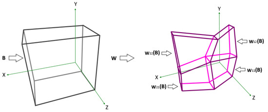
Figure 1. A collage map $W:\mathcal{H}\left({\mathbb{R}}^3\right)\to \mathcal{H}\left({\mathbb{R}}^3\right)$ for $M=N=2$.

From [9], we have the following.

Theorem 1.

Let $\{X;w_{1-N,1-M}\}$ be a hyperbolic IFS with contractivity factor $s=max\{s_{m,n}:m=1,2,\dots ,M;n=1,2,\dots ,N\}.$ The transformation $W:\mathcal{H}\left(X\right)\to \mathcal{H}\left(X\right)$, where

$$W\left(B\right)=\bigcup _{m=1}^M\bigcup _{n=1}^N{w}_{m,n}\left(B\right),for all B\in \mathcal{H}\left(X\right),$$

is a contraction mapping of the complete metric space $\left(\mathcal{H}\right(X),h(\rho \left)\right)$ with contractivity factor s. The unique compact set $\mathcal{A}\in \mathcal{H}\left(X\right)$ satisfies

$$\mathcal{A}=W\left(\mathcal{A}\right)=\bigcup _{m=1}^M\bigcup _{n=1}^N{w}_{m,n}\left(\mathcal{A}\right),$$

is called the attractor of the hyperbolic IFS and it is equal to

$$\mathcal{A}=\underset{k\to \infty }{lim}{W}^k\left(B\right),for all B\in \mathcal{H}\left(X\right).$$

5.3. Identifying the Vertical Scaling Factors

Let $B\in K_0^3$ be the convex bounding volume of P and $B_{m,n}\in K_0^3$ be the convex bounding volumes of $P_{m,n}$. The parameters $s_{m,n}$ must be computed in such a way as to derive maximum overlap between the corresponding bounding volumes. The objective is to minimise the volume of the non-overlapping parts of the convex hull of the set $P_{m,n}$ and the transformed by $w_{m,n}$ convex hull of the set P, for all $m=1,2,\dots ,M$ and $n=1,2,\dots ,N$. That corresponds to the minimisation of the symmetrical distance:

$$\begin{array}{c}{\delta }_s(CH\left(P_{m,n}\right),w_{m,n}\left(CH\left(P\right)\right))\hfill \\ =Volume\left\{CH\left(P_{m,n}\right)\right\}+Volume\left\{w_{m,n}\left(CH\left(P\right)\right)\right\}-2·Volume\{CH\left(P_{m,n}\right)\cap w_{m,n}\left(CH\left(P\right)\right)\}\hfill \\ =Volume\left\{CH\left(P_{m,n}\right)\right\}+Volume\left\{w_{m,n}\left(CH\left(P\right)\right)\right\}-2·Volume\left\{CH(P_{m,n}\cap w_{m,n}\left(P\right))\right\}\hfill \end{array}$$

(1)

Since $w_{m,n}$ are affine, it implies that $w_{m,n}\left(CH(·)\right)=CH\left(w_{m,n}(·)\right)$. As implied by Equation (1), the calculation of ${\delta }_S$ is algorithmic and involves the computation of convex hulls, intersections of polyhedra and volumes. Therefore, a method for two-dimensional minimisation without derivatives should be used, such as Brent’s method [17], which is a bracketing method with parabolic interpolation. Initially, for the method to converge to optimum ${\widehat{s}}_{m,n}^{+}$, we must initially bracket it, i.e., provide three constants $s_{m,n}^a,s_{m,n}^b,s_{m,n}^c$, such that

$$\begin{gathered} 0\le s_{m,n}^a<s_{m,n}^b<s_{m,n}^c\le 1, \\ Vol\left(s_{m,n}^b\right)<Vol\left(s_{m,n}^a\right),Vol\left(s_{m,n}^b\right)<Vol\left(s_{m,n}^c\right), \\ {s}_{m,n}^a<{\widehat{s}}_{m,n}^{+}<s_{m,n}^c. \end{gathered}$$

A good approximation is to estimate $s_{m,n}^b$ such that

$$Vol\left\{w_{m,n}\left(CH\left(P\right)\right)\right\}\approx Vol\left\{CH\left(P_{m,n}\right)\right\}.$$

Next $s_{m,n}^a,s_{m,n}^c$ follow from $s_{m,n}^b$, respectively, by a factor, that is

$$\begin{array}{c}{s}_{m,n}^b=Vol\{CH\left(P_{m,n}\right\}/(a_{m,n}·c_{m,n}·Vol\left\{CH\left(P\right)\right\}),\hfill \\ s_{m,n}^a=s_{m,n}^b/c,\hfill \\ s_{m,n}^c=min\{c{s}_{m,n}^b,1\},\hfill \end{array}$$

for some $c>1$. The constant c can be determined a priori, e.g., $c=2$, or more safely using an iterative procedure of checking successively larger values until a suitable bracketing triplet is found. In cases of negative factors, the optimum ${\widehat{s}}_{m,n}^{-}$ can be similarly calculated by using the bracketing triplet

$$\begin{array}{c}{s}_{m,n}^{b^{\prime }}=-s_{m,n}^b,\hfill \\ s_{m,n}^{a^{\prime }}=max\{c{s}_{m,n}^{b^{\prime }},-1\},\hfill \\ s_{m,n}^{c^{\prime }}=s_{m,n}^{b^{\prime }}/c.\hfill \end{array}$$

The algorithm for finding the optimum vertical scaling factors can be outlined in Listing 4.

Listing 4. Calculation of the optimum vertical scaling factors of FIS.

Compute the convex hull of the set of the data points P. For each subdomain $D_{m,n}$, where $m=1,2,\dots ,M$ and $n=1,2,\dots ,N$ 2.1. Compute the known parameters $a_{m,n}$, $b_{m,n}$, $c_{m,n}$, $d_{m,n}$, $e_{m,n}$, $f_{m,n}$, $g_{m,n}$, $k_{m,n}$ of the transformation $w_{m,n}$ 2.2. Compute the convex hull of the set $P_{m,n}$ 2.3. Find the optimum ${\widehat{s}}_{m,n}^{+}\in [0,1)$ that minimise the volume of non-overlapping parts of volumes $CH\left(P_{m,n}\right)$ and $w_{m,n}\left(CH\left(P\right)\right)$, using the bracketing triplet $(s_{m,n}^b/c,s_{m,n}^b,min\{c{s}_{m,n}^b,1\})$, where $c>1$ and $s_{m,n}^b=Volume\left\{CH\left(P_{m,n}\right)\right\}/a_{m,n}·c_{m,n}·Volume\left\{CH\left(P\right)\right\}$ 2.4. Find the optimum ${\widehat{s}}_{m,n}^{-}\in (-1,0]$ that minimise the volume of non-overlapping parts of volumes $CH\left(P_{m,n}\right)$ and $w_{m,n}\left(CH\left(P\right)\right)$, using the bracketing triplet $(max\{c{s}_{m,n}^{b^{\prime }},-1\},s_{m,n}^{b^{\prime }},s_{m,n}^{b^{\prime }}/c)$, where $c>1$ and $s_{m,n}^{b^{\prime }}=-s_b$ 2.5. If $Volume\left\{{\widehat{s}}_{m,n}^{+}\right\}\le Volume\left\{{\widehat{s}}_{m,n}^{-}\right\}$, then ${\widehat{s}}_{m,n}={\widehat{s}}_{m,n}^{+}$, else ${\widehat{s}}_{m,n}={\widehat{s}}_{m,n}^{-}$

The calculation of a vertical scaling factor $s_{m,n}$ depends on the number of data points within the respective interpolation interval surface, while in the worst case scenario it requires time $O(Klog\left(K\right)/(M·N\left)\right)$. Since there are $M·N$ factors $s_{m,n}$, the worst-case computational complexity of the algorithm is proportionate to the number of the data points, i.e., $O(Klog\left(K\right))$. Moreover, convex hulls usually have few vertices, so calculations are quick. Figure 2 shows the results of three examples of fractal interpolation according to the proposed methodologies.

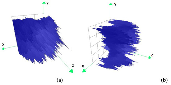
Figure 2. Example of fractal interpolation for (a) $3\times 3$, (b) $4\times 4$, partitions of the $XY$ plane.

6. Examples and Discussion

In this section, examples for finding the convex hull of a set of points, calculating the volume of a convex polyhedron and determining the intersection of two convex polyhedra, and finally identifying the parameters of two-dimensional fractal interpolation functions by using bounding volumes are presented and discussed. The implementation of the proposed algorithms and their integration into a software tool were written in the C++ programming language by using $Microsof{t}^{\circledR }VisualStudi{o}^{\circledR }$ IDE. The library CGAL was extensively used together with the DirectX library for the three-dimensional representation of the results.

The most common algorithm to compute fractals derived by IFSs is called the chaos game or random iteration algorithm. It consists of picking a random point in the plane, then iteratively applying one of the functions chosen at random from the function system and drawing the point. An alternative algorithm, the deterministic iteration algorithm, or DIA for short, is to generate each possible sequence of functions up to a given maximum length and then to plot the results of applying each of these sequences of functions to an initial point or shape.

As an initial data set of points for $2\times 2$ partitioning of the $XY$ plane, the points in Table 1a are used. The interpolation points corresponding to this original data set are listed in Table 1b. Figure 3 corresponds to the original mesh of the interpolation points of the example, while Figure 4 corresponds to the convex hull of the original data set, calculated with the Quickhull algorithm.

Table 1. (a) The initial data set for $2\times 2$ partitioning of the $XY$ plane, (b) the correspong interpolation points.

(a)			(b)
x	y	z		x
			y	0	0.5	1
0.00	0.00	0.20	0	0.2	0.2	0.2
0.00	0.50	0.20	0.5	0.2	1.0	0.2
0.00	1.00	0.20	1	0.2	0.2	0.2
0.25	0.25	0.50
0.25	0.75	0.80
0.50	0.00	0.20
0.50	0.50	1.00
0.50	1.00	0.20
0.75	0.25	0.80
0.75	0.75	0.50
1.00	0.00	0.20
1.00	0.50	0.20
1.00	1.00	0.20

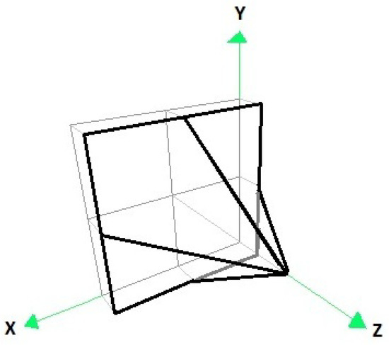
Figure 3. The original grid of interpolation points (2 × 2 partition).

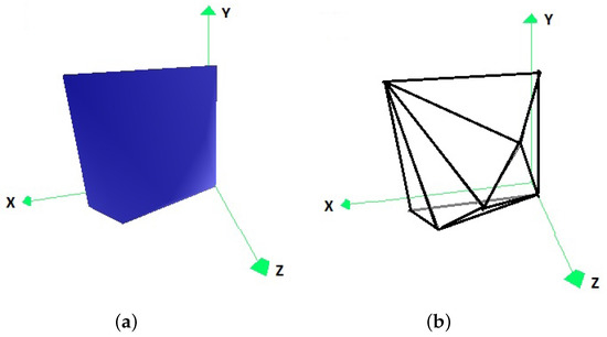
Figure 4. The convex hull of the original data set (a) in the form of coloured vertices, and (b) with its edge representation.

To calculate the optimal factors $s_{m,n}$, with $m=1.2$ and $n=1.2$ of each subdomain of the example, according to the algorithm presented in Section 5.3, the factors that minimize the volume of the non-overlapping parts of the convex hull of the set $P_{m,n}$ and of the convex hull of the set P transformed by $w_{m,n}$ for each $m=1,2$ and $n=1,2$ must be chosen. The convex hulls of $P_{m,n}$, for each $m=1,2$ and $n=1,2$, of the subdomains of the example, are represented in Figure 5, Figure 6, Figure 7 and Figure 8.

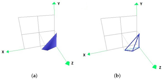
Figure 5. The convex hull of the original data set $P_{1,1}$ (a) in the form of coloured vertices, and (b) with its edge representation.

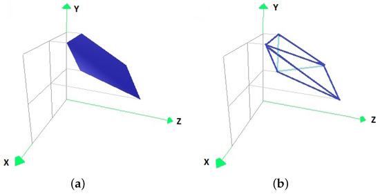
Figure 6. The convex hull of the original data set $P_{1,2}$ (a) in the form of coloured vertices, and (b) with its edge representation.

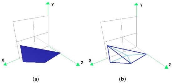
Figure 7. The convex hull of the original data set $P_{2,1}$ (a) in the form of coloured vertices, and (b) with its edge representation.

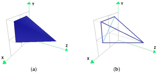
Figure 8. The convex hull of the original data set $P_{2,2}$ (a) in the form of coloured vertices, and (b) with its edge representation.

By applying the algorithm for finding the optimal factors $s_{m,n}$, for $m=1,2$ and $n=1,2$, the factors listed in Table 2 are obtained. Based on these optimal factors, the transformed points for each sub-region are calculated, with their convex hulls depicted in Figure 9, Figure 10, Figure 11 and Figure 12.

Table 2. (a) Optimum factors $s_{m,n}$ for $m=1,2$ and $n=1,2$, and (b) symmetric differences of subdomains $(m,n)$.

(a)			(b)
	m			m
n	1	2	n	1	2
1	0.05	0.60	1	0.0	0.0125
2	0.60	0.05	2	0.0125	0.0

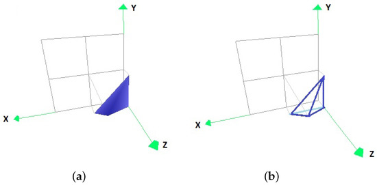
Figure 9. The convex hull of the points resulting from the transformation of the vertices of the convex hull of the set P by $w_{1,1}$ (a) in the form of coloured faces, and (b) in its edge representation.

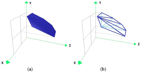
Figure 10. The convex hull of the points resulting from the transformation of the vertices of the convex hull of the set P by $w_{1,2}$ (a) in the form of coloured faces, and (b) in its edge representation.

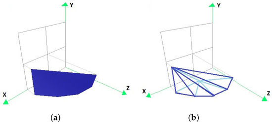
Figure 11. The convex hull of the points resulting from the transformation of the vertices of the convex hull of the set P by $w_{2,1}$ (a) in the form of coloured faces, and (b) in its edge representation.

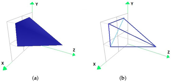
Figure 12. The convex hull of the points resulting from the transformation of the vertices of the convex hull of the set P by $w_{2,2}$ (a) in the form of coloured faces, and (b) in its edge representation.

Their intersections with the corresponding convex hulls of $Pm,n$, for each $m=1,2$ and $n=1,2$, are illustrated in Figure 13, Figure 14, Figure 15 and Figure 16.

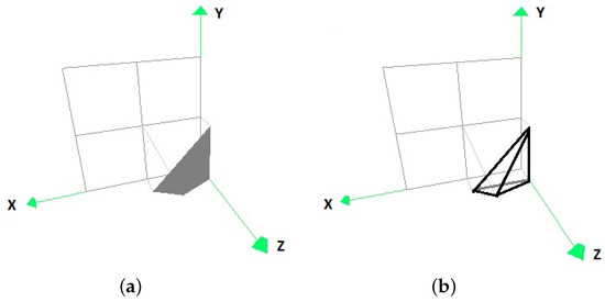
Figure 13. The intersection of the convex hull of the original data set $P_{1,1}$ with the convex hull of the points resulting from the transformation of the vertices of the convex hull of the set P by $w_{1,1}$ (a) in the form of coloured faces, and (b) with its edge representation.

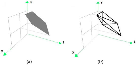
Figure 14. The intersection of the convex hull of the original data set $P_{1,2}$ with the convex hull of the points resulting from the transformation of the vertices of the convex hull of the set P by $w_{1,2}$ (a) in the form of coloured faces, and (b) with its edge representation.

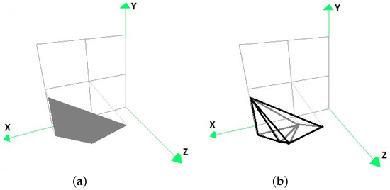
Figure 15. The intersection of the convex hull of the original data set $P_{2,1}$ with the convex hull of the points resulting from the transformation of the vertices of the convex hull of the set P by $w_{2,1}$ (a) in the form of coloured faces, and (b) with its edge representation.

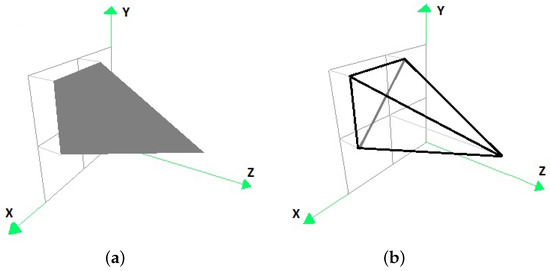
Figure 16. The intersection of the convex hull of the original data set $P_{2,2}$ with the convex hull of the points resulting from the transformation of the vertices of the convex hull of the set P by $w_{2,2}$ (a) in the form of coloured faces, and (b) with its edge representation.

The symmetric differences of the convex hulls of $P_{m,n}$, for each $m=1,2$ and $n=1,2$ with the convex hulls of the points resulting from the transformations of the vertices of the convex hull of the set P by $w_{m,n}$, for each $m=1,2$ and $n=1,2$, respectively, are presented in Table 2b. The fractal interpolation image constructed with five iterations of the DIA is shown under two different viewing angles in Figure 17 and Figure 18.

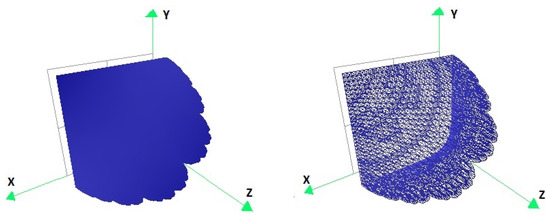
Figure 17. Fractal interpolation function for the example with $2\times 2$ partitioning of the $XY$ plane.

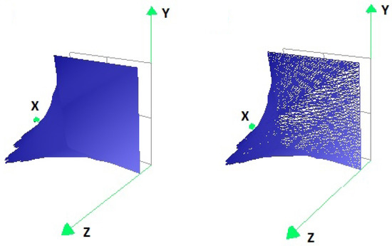
Figure 18. Fractal interpolation function for the example with $2\times 2$ partitioning of the $XY$ plane.

7. Conclusions

The subject of this study is the theoretical study and implementation of algorithms for convex polyhedra and their application in the field of fractal interpolation. The goal is, by finding and implementing efficient algorithms for convex polyhedra, the computation of parameters and the algorithmic construction of bivariate fractal interpolation functions using bounding volumes. Several methods for computing the convex hull of an initial set of points, calculating the volume of a convex polyhedron and finding the intersection of two convex polyhedra are presented and analysed. In the selection of a pre-existing algorithm (convex hull) as well as in the introduction of new algorithms (volume and intersection), special emphasis was placed on their efficiency.

Furthermore, we present a methodology for constructing continuous fractal interpolation surfaces, which uses the above algorithms for identifying non-free parameters, while it is based on iterated function systems. Given a set of points in three-dimensional space ${\mathbb{R}}^3$, a subset of them is selected as interpolation points and a fractal representation is constructed which passes through them. The identification of the parameters (free or not) of such a representation is important as is determines the quality of interpolation with respect to the initial set of points. We present a new method of identifying non-free parameters, extending in ${\mathbb{R}}^3$ an existing one in $R2$. The proposed methodology is based on minimising the symmetric difference between the bounding volumes of appropriately chosen points, and it achieves a lower error in the accuracy of the result.

These algorithms are applied to identify the parameters, and thus in the algorithmic construction of bivariable fractal interpolation functions by using bounding volumes. An algorithm for calculating the vertical scaling factors of fractal interpolation surfaces, such as to achieve optimal representation of the data points was proposed and implemented. In the procedure of constructing a fractal interpolation surface, the main difficulty that had to be addressed was to ensure continuity. The proposed methodology is limited to convex bounding volumes, since it is uncertain whether non-convex can be combined with efficient algorithms or improve the results. This will be the subject of our potential future research.

References

- Barnsley, M.F. Fractal functions and interpolation. Constr. Approx. 1986, 2, 303–329. [Google Scholar] [CrossRef]
- Barnsley, M.F. Fractals Everywhere, 3rd ed.; Dover Publications, Inc.: New York, NY, USA, 2012. [Google Scholar]
- Massopust, P.R. Fractal surfaces. J. Math. Anal. Appl. 1990, 151, 275–290. [Google Scholar] [CrossRef]
- Geronimo, J.S.; Hardin, D. Fractal interpolation surfaces and a related 2-D multiresolution analysis. J. Math. Anal. Appl. 1993, 176, 561–586. [Google Scholar] [CrossRef]
- Zhao, N. Construction and application of fractal interpolation surfaces. Vis. Comput. 1996, 12, 132–146. [Google Scholar] [CrossRef]
- Massopust, P.R. Fractal Functions, Fractal Surfaces and Wavelets; Academic Press: San Diego, CA, USA, 1994. [Google Scholar]
- Qian, X.Y. Bivariate fractal interpolation functions on rectangular domains. J. Comp. Math. 2002, 20, 349–362. [Google Scholar]
- Wang, H.Y. On smoothness for a class of fractal interpolation surfaces. Fractals 2006, 14, 223–230. [Google Scholar] [CrossRef]
- Drakopoulos, V.; Manousopoulos, P. On non-tensor product bivariate fractal interpolation surfaces on rectangular grids. Mathematics 2020, 8, 525. [Google Scholar] [CrossRef]
- Xie, H.; Sun, H.; Ju, Y.; Feng, Z. Study on generation of rock fracture surfaces by using fractal interpolation. Int. J. Solids Struct. 2001, 38, 5765–5787. [Google Scholar] [CrossRef]
- Sun, H.; Xie, H. Study on the improved fractal interpolation surface of the attitude and surface fault. In Thinking in Patterns; Novak, M.M., Ed.; World Scientific: Singapore, 2004; pp. 243–254. [Google Scholar]
- Bouboulis, P.; Dalla, L.; Drakopoulos, V. Construction of recurrent bivariate fractal interpolation surfaces and computation of their box-counting dimension. J. Approx. Theory 2006, 141, 99–117. [Google Scholar] [CrossRef]
- Verma, S.; Viswanathan, P. Parameter Identification for a Class of Bivariate Fractal Interpolation Functions and Constrained Approximation. Numer. Funct. Anal. Optim. 2020, 41, 1109–1148. [Google Scholar] [CrossRef]
- Manousopoulos, P.; Drakopoulos, V.; Theoharis, T. Parameter identification of 1D fractal interpolation functions using bounding volumes. J. Comput. Appl. Math. 2009, 233, 1063–1082. [Google Scholar] [CrossRef]
- Clarkson, K.; Shor, P. Applications of random sampling in computational geometry, i. Disc. Comput. Geom. 1989, 4, 387–421. [Google Scholar] [CrossRef]
- Barber, C.B.; Dobkin, D.P.; Huhdanpaa, H. The quickhull algorithm for convex hulls. ACM Trans. Math. Softw. 1996, 22, 469–483. [Google Scholar] [CrossRef]
- Press, W.H.; Teukolsky, S.A.; Vetterling, W.T.; Flannery, B.P. Numerical Recipes in C (2nd ed.): The Art of Scientific Computing; Cambridge University Press: Cambridge, MA, USA, 1992. [Google Scholar]
Disclaimer/Publisher’s Note: The statements, opinions and data contained in all publications are solely those of the individual author(s) and contributor(s) and not of MDPI and/or the editor(s). MDPI and/or the editor(s) disclaim responsibility for any injury to people or property resulting from any ideas, methods, instructions or products referred to in the content. |
© 2023 by the authors. Licensee MDPI, Basel, Switzerland. This article is an open access article distributed under the terms and conditions of the Creative Commons Attribution (CC BY) license (https://creativecommons.org/licenses/by/4.0/).