Transient Dynamic Response Analysis of Two-Dimensional Saturated Soil with Singular Boundary Method

Abstract

In this paper, the singular boundary method (SBM) in conjunction with the exponential window method (EWM) is firstly extended to simulate the transient dynamic response of two-dimensional saturated soil. The frequency-domain (Fourier space) governing equations of Biot theory is solved by the SBM with a linear combination of the fundamental solutions. In order to avoid the perplexing fictitious boundary in the method of fundamental solution (MFS), the SBM places the source point on the physical boundary and eliminates the source singularity of the fundamental solution via the origin intensity factors (OIFs). The EWM is carried out for the inverse Fourier transform, which transforms the frequency-domain solutions into the time-domain solutions. The accuracy and feasibility of the SBM-EWM are verified by three numerical examples. The numerical comparison between the MFS and SBM indicates that the SBM takes a quarter of the time taken by the MFS.

1. Introduction

The transient dynamic analysis is of great importance in the geotechnical and mechanical engineering to observe the time-history mechanical response caused by the dynamic loads [1,2]. Although there are some analytical solutions for the regular geometric shapes with isotropic and homogeneous material properties and simple boundary conditions, the numerical tools are usually more flexible and effective for general real-world problems. The transient analysis is usually divided into two parts, viz. spatial discretization and temporal discretization.

For the spatial discretization, the finite element method (FEM) is one of most powerful numerical methods. In light of its theoretical completeness and well-established commercial software, the FEM is robust to different engineering applications [3,4]. Nevertheless, the FEM requires the artificial boundary [5] to analyze the infinite and semi-infinite medium. Besides the FEM, the other domain-type methods [6] encounter the same difficulty. The boundary element method (BEM) has been boosted as an effective alternative in infinite and semi-infinite problems because the fundamental solutions used in the BEM automatically satisfy the Sommerfield radiation condition at infinity. The utilization of the fundamental solutions makes the BEM avoid domain discretization, because the kernel function satisfies governing equations. The superiority of the BEM motivated researchers to develop novel numerical methods based on analytical solutions, such as the fundamental solutions [7,8,9], the general solutions [10,11,12] and the particular solutions [13,14,15,16]. Among them, most of numerical methods are pertinent to the fundamental solutions, including the method of fundamental solutions (MFS) [8,17], modified method of fundamental solutions [18] and singular boundary method (SBM) [19,20,21], to just name a few. The SBM was firstly proposed by Chen [19] with introducing the concept of the origin intensity factor (OIF) to desingularize the fundamental solutions. Originally, the OIF was evaluated via a tedious inverse interpolation technique [22]. Later, simple analytical and empirical formulas were developed and extended the application of the SBM to different problems [23,24,25,26,27,28,29,30,31,32]. The abovementioned boundary-type methods required expensive operation counts and memory storage in real-world large-scale problems. This promotes the development of fast algorithms accelerated techniques [33,34,35,36,37] and localized methods [38,39,40,41]. It is worth noting that the localized variant of the boundary-type method is a domain-type method.

To implement the transient analysis, the boundary methods require special treatment to deal with time-dependent terms, including the direct time integration methods [42,43,44], transform methods [45,46,47] and time-domain fundamental solutions [48]. Except the transform method, the other methods require a proper time-step for numerical stability. Nevertheless, the long-time solution may deteriorate as the time increases. The Krylov deferred correction method (KDC) [49] allows larger time step size for the long-time analysis with acceptable temporal accumulation errors. In the transform methods, the frequency-domain governing equation is solved at some discrete sampling frequencies, and then the frequency-domain solutions are transformed back to the time-domain solutions via the inverse transform, namely the Laplace transform or Fourier transform. The inverse transform is carried out by numerical methods, which may consume a lot of time. The Fourier transform is more attractive because its inverse process can be accelerated by the fast Fourier transform (FFT). However, in lightly damped systems or undamped systems, the FFT is inefficient, or even not applicable without the desired attenuation. This problem was circumvented by introducing an artificial damping to the system by the exponential window method (EWM) [50].

There are few works related to the transient dynamic response analysis of saturated soil. In this study, the SBM in conjunction with the EWM is firstly established to solve the transient dynamic problems in two-dimensional saturated soil. The SBM is formulated in the frequency domain (Fourier space). Thanks to the fundamental solutions, the SBM can be directly applied to finite-, semi-infinite and infinite domains. The source singularity of the fundamental solution is bypassed with simple formulas. Subsequently, the frequency-domain SBM solutions are transformed by the EWM. The selection of the parameters in the EWM will be discussed. The stability and accuracy of the SBM will be investigated via three numerical examples.

2. Governing Equations

For the saturated soil, it is better to take the coupling effect of two phases into consideration [51,52]. Thus, the coupling effect is taken into account in the constitute equation [53,54]:

$${\sigma }_{ij}=\lambda {\delta }_{ij}{u}_{k,k}+2\mu {\epsilon }_{ij}-\alpha {\delta }_{ij}p,\hspace{1em}i=1,3,j=1,3,$$

(1)

$$p=-\alpha M{u}_{i,i}-M{w}_{i,i},$$

(2)

where ${\sigma }_{ij}$ is the effective stress; ${\delta }_{ij}$ the Kronecker delta; ${\epsilon }_{ij}=\left(u_{i,j}+u_{j,i}\right)/2$ the strain tensor; $w_i$ the fluid displacement with respect to the solid skeleton; $p$ the pore pressure; $u_i$ the average skeleton displacement; $\lambda$ and $\mu$ the solid skeleton Lamé constants; and $\alpha$ and $M$ the Biot parameters describing the compressibility of the fluid-saturated two-phase material.

Taking Equations (1) and (2) into the equilibrium equations, we obtained the equations of motion for the bulk porous medium and the pore fluid without body forces as [53,54]

$$\mu u_{i,jj}+\left(\lambda +{\alpha }^{2}M+\mu \right)u_{j,ji}+\alpha M{w}_{j,ji}=\rho {\ddot{u}}_i+{\rho }_f{\ddot{w}}_i,$$

(3)

$$\alpha M{u}_{j,ji}+M{w}_{j,ji}={\rho }_f{\ddot{u}}_i+m{\ddot{w}}_i+\frac{\eta }{k}K\left(t\right)\ast {\dot{w}}_i,$$

(4)

where a dot $(•)$ denotes the time derivative and a star $(\ast )$ denotes the time convolution; $\rho =\left(1-\varphi \right){\rho }_s+\varphi {\rho }_f$ is the density of the saturated poroelastic medium; ${\rho }_s$ and ${\rho }_f$ are the density of the skeleton and fluid; $\varphi$ the porosity; $\eta$ the viscosity of the pore fluid; $k$ the permeability of the saturated poroelastic medium; $m={\alpha }_{\infty }{\rho }_f/\varphi$; ${\alpha }_{\infty }$ is the tortuosity; and $K\left(t\right)$ is a time-dependent viscosity correction factor which describes the transition between the viscous flow in the low-frequency range and the inertia-dominated flow in the high-frequency range.

The initial boundary conditions and boundary conditions are given as

$${{\mathit{u}}^s|}_{t=0}={\frac{\partial {\mathit{u}}^s}{\partial t}|}_{t=0}=0,{\mathit{w}|}_{t=0}=0,\hspace{0.17em}\mathrm{and}\hspace{0.17em}{p|}_{t=0}=0,$$

(5)

$$u_i^s={\widehat{u}}_i^s,\hspace{0.17em}\mathrm{on}\hspace{0.17em}{\Gamma }_u^s,$$

(6)

$$t_i^s={\sigma }_{i1}^s{n}_1+{\sigma }_{i3}^s{n}_3={\widehat{t}}_i^s,\hspace{0.17em}\hspace{0.17em}\mathrm{on}\hspace{0.17em}{\Gamma }_t^s,$$

(7)

$$w_i={\widehat{w}}_i,\hspace{0.17em}\hspace{0.17em}\mathrm{on}\hspace{0.17em}{\Gamma }_w^f,$$

(8)

$$p=\widehat{p},\hspace{0.17em}\hspace{0.17em}\mathrm{on}\hspace{0.17em}{\Gamma }_p^f,$$

(9)

where $\mathit{n}=(n_1,n_3)$ is the normal vector to the boundary, and ${\widehat{u}}_i^s$, ${\widehat{t}}_i^s$, ${\widehat{w}}_i$ and $\widehat{p}$ are the prescribed solid displacements, tractions, relative fluid displacements and pore pressure on the boundary, respectively.

We introduce the Fourier transform with respect to time and frequency as

$$\tilde{f}\left(\omega \right)={\displaystyle {\int }_{-\infty }^{+\infty }f\left(t\right)e^{-\mathrm{j}\omega t}}dt,\hspace{1em}f\left(t\right)=\frac{1}{2\pi }{\displaystyle {\int }_{-\infty }^{+\infty }\tilde{f}\left(\omega \right)e^{\mathrm{j}\omega t}}d\omega ,$$

(10)

where $\mathrm{j}=\sqrt{-1}$ is the imaginary unit.

After Fourier transform on Equations (3) and (4), the frequency-domain governing equations in terms of solid displacement and fluid pressure [54] are recast as

$$\mu {\tilde{u}}_{i,jj}+\left(\lambda +\mu \right){\tilde{u}}_{j,ji}+{\rho }_g{\omega }^2{\tilde{u}}_i-{\alpha }_g{\tilde{p}}_{,i}=0,\hspace{1em}$$

(11)

$${\tilde{p}}_{,jj}+{\beta }_2{\omega }^2\tilde{p}-{\beta }_3{\tilde{u}}_{j,j}=0,$$

(12)

where ${\rho }_g=\rho -{\beta }_4{\rho }_f$, ${\alpha }_g=\alpha -{\beta }_4$, ${\beta }_1=M/\left[m{\omega }^2-\mathrm{j}\omega \left(\eta /k\right)\tilde{K}\left(\omega \right)\right]$, ${\beta }_2=1/\left({\beta }_1{\omega }^2\right)$, ${\beta }_4={\rho }_f{\omega }^2{\beta }_1/M$; ${\beta }_3={\rho }_f{\omega }^2-\alpha \left[m{\omega }^2-\mathrm{j}\omega \left(\eta /k\right)\tilde{K}\left(\omega \right)\right]$, $\tilde{K}\left(\omega \right)$ is the Fourier transform of $K\left(t\right)$, and “~” denotes the representation in the frequency-domain.

3. Singular Boundary Method in Frequency-Domain

In this section, the SBM formulation is established for the frequency-domain governing equations. The SBM evaluates the frequency-domain solution with a linear combination of fundamental solutions in terms of the source points as [55]

$${\tilde{u}}_i^s\left({\mathit{x}}_m\right)={\displaystyle \sum _{n=1}^N{\beta }_{1n}{\tilde{u}}_{i1}^s}\left({\mathit{x}}_m,{\mathit{s}}_n\right)+{\displaystyle \sum _{n=1}^N{\beta }_{3n}{\tilde{u}}_{i3}^s}\left({\mathit{x}}_m,{\mathit{s}}_n\right)+{\displaystyle \sum _{n=1}^N{\beta }_{4n}{\tilde{u}}_{i4}^s}\left({\mathit{x}}_m,{\mathit{s}}_n\right),\hspace{1em}i=1,3,$$

(13)

$$\tilde{p}\left({\mathit{x}}_m\right)={\displaystyle \sum _{n=1}^N{\beta }_{1n}}{\tilde{p}}_1\left({\mathit{x}}_m,{\mathit{s}}_n\right)+{\displaystyle \sum _{n=1}^N{\beta }_{3n}}{\tilde{p}}_3\left({\mathit{x}}_m,{\mathit{s}}_n\right)+{\displaystyle \sum _{n=1}^N{\beta }_{4n}}{\tilde{p}}_4\left({\mathit{x}}_m,{\mathit{s}}_n\right),$$

(14)

$${\tilde{t}}_i^s\left({\mathit{x}}_m\right)={\displaystyle \sum _{n=1}^N{\beta }_{1n}{\tilde{t}}_{i1}^s}\left({\mathit{x}}_m,{\mathit{s}}_n\right)+{\displaystyle \sum _{n=1}^N{\beta }_{3n}{\tilde{t}}_{i3}^s}\left({\mathit{x}}_m,{\mathit{s}}_n\right)+{\displaystyle \sum _{n=1}^N{\beta }_{4n}{\tilde{t}}_{i4}^s}\left({\mathit{x}}_m,{\mathit{s}}_n\right),\hspace{1em}i=1,3,$$

(15)

$${\tilde{q}}_{\mathbf{n}}\left({\mathit{x}}_m\right)={\displaystyle \sum _{n=1}^N{\beta }_{1n}}{\tilde{q}}_1\left({\mathit{x}}_m,{\mathit{s}}_n\right)+{\displaystyle \sum _{n=1}^N{\beta }_{3n}}{\tilde{q}}_3\left({\mathit{x}}_m,{\mathit{s}}_n\right)+{\displaystyle \sum _{n=1}^N{\beta }_{4n}}{\tilde{q}}_4\left({\mathit{x}}_m,{\mathit{s}}_n\right).$$

(16)

where ${\mathit{x}}_m,{\mathit{s}}_n$ are the mth field point and nth source point; N is the total number of boundary source points; ${\left\{{\beta }_{kn}\right\}}_{n=1}^N\left(k=1,3,4\right)$ are the coefficients to be determined; and ${\tilde{u}}_{ik}^s$, ${\tilde{t}}_{ik}^s$, ${\tilde{p}}_k$ and ${\tilde{q}}_k$ $\left(i=1,3, k=1,3,4\right)$ are the fundamental solutions of solid displacements, traction, pore pressure and flux, which are given as

$${\tilde{u}}_{ik}^s=A{\delta }_{ik}-B{r}_{,i}{r}_{,k}, {\tilde{u}}_{i4}^s=D{r}_{,i}, i,k=1,3,$$

(17)

$$\begin{array}{l}{\tilde{t}}_{ik}^s=\lambda \left[A^{\prime }-B^{\prime }-\frac{B}{r}\right]r_{,k}{n}_i+\mu [\left(A^{\prime }-\frac{B}{r}\right)\left(r_{,n}{\delta }_{ik}+r_{,i}{n}_k\right)\\ \hspace{1em}-\frac{2B}{r}{r}_{,k}{n}_i+2\left(-B^{\prime }+\frac{2B}{r}\right)r_{,i}{r}_{,k}{r}_{,n}], i,k=1,3,\\ {\tilde{t}}_{i4}^s=\left[\left(\lambda +2\mu \right)\frac{D}{r}+\lambda D^{\prime }\right]n_i+2\mu \left(-\frac{D}{r}+D^{\prime }\right)r_{,i}{r}_{,n}, i=1,3,\end{array}$$

(18)

$${\tilde{p}}_k=C{r}_{,k},\hspace{0.17em}{\tilde{p}}_4=\frac{1}{2\pi }{\displaystyle \sum _{d=1,2}{r}_d{h}_d{K}_0}\left(z_d\right), k=1,3,$$

(19)

$${\tilde{q}}_k=\{\begin{array}{l}\frac{-{\alpha }_g}{{\beta }_3}\left[\frac{C}{r}{n}_k+\left(C^{\prime }-\frac{C}{r}\right)r_{,k}{r}_{,n}\right], k=1,3,\\ \frac{\mathrm{j}{\alpha }_g{r}_{,n}}{2\pi {\beta }_3}{\displaystyle \sum _{d=1,2}{r}_d{h}_d{k}_d{K}_1\left(z_d\right), k=4,}\end{array}$$

(20)

where

$$A=\frac{1}{2\pi }\left[-{\displaystyle \sum _{d=1,2}{g}_d\frac{K_1\left(z_d\right)}{z_d}+g_3\left(K_0\left(z_3\right)+\frac{K_1\left(z_3\right)}{z_3}\right)}\right], C=\frac{\mathrm{j}}{2\pi }\left[{\displaystyle \sum _{d=1,2}\frac{r_d{g}_d}{k_d}{K}_1\left(z_d\right)}\right]$$

$$B=\frac{1}{2\pi }\left[-{\displaystyle \sum _{d=1,2}{g}_d{K}_2\left(z_d\right)+g_3{K}_2\left(z_3\right)}\right], D=\frac{-\mathrm{j}}{2\pi }{\displaystyle \sum _{d=1,2}{k}_d}{h}_d{K}_1\left(z_d\right)z_3=\mathrm{j}{k}_{3}r$$

$$z_d=\mathrm{j}{k}_{d}r, r_d=\frac{{\omega }^2{\rho }_g-\left(\lambda +2\mu \right)k_d^2}{{\alpha }_g}\left(d=1,2\right),\hspace{0.17em} g_1=\frac{{\beta }_3-r_2}{\left(\lambda +2\mu \right)\left(r_1-r_2\right)},$$

$$g_2=\frac{{\beta }_3-r_1}{\left(\lambda +2\mu \right)\left(r_2-r_1\right)}, g_3=\frac{1}{\mu }, h_1=-\frac{{\beta }_3}{{\alpha }_g\left(r_1-r_2\right)}, h_2=-\frac{{\beta }_3}{{\alpha }_g\left(r_2-r_1\right)}$$

in which $r=\sqrt{{\left(x_1-y_1\right)}^2+{\left(x_3-y_3\right)}^2}$ is the distance between field point $\mathit{x}$ = (x₁, x₃) and source point $\mathit{y}$ = (y₁, y₃). $K_n$ is the modified Bessel function of the second kind of order n, and $k_d$ is

$$k_1=\sqrt{\frac{{\beta }_2{\omega }^2}{2}+\frac{{\rho }_g{\omega }^2-{\alpha }_g{\beta }_3+\sqrt{H}}{2\left(\lambda +2\mu \right)}}, k_2=\sqrt{\frac{{\beta }_2{\omega }^2}{2}+\frac{{\rho }_g{\omega }^2-{\alpha }_g{\beta }_3-\sqrt{H}}{2\left(\lambda +2\mu \right)},} k_3=\sqrt{{\omega }^2{\rho }_g/\mu }$$

where

$$H={\left(\lambda {\beta }_2{\omega }^2-{\alpha }_g{\beta }_3+{\rho }_g{\omega }^2\right)}^2+4\left(\lambda +\mu \right){\beta }_2{\omega }^4\left(\mu {\beta }_2-{\rho }_g\right)-4\mu {\alpha }_g{\beta }_2{\beta }_3{\omega }^2$$

The derivation of the fundamental solutions is detailed in Appendix A.

With the fundamental solutions, Equations (13)–(16) are forced to satisfy the boundary conditions for the determination of the unknown coefficients. Then the boundary conditions with Equations (13)–(16) are formulated as

$${\tilde{u}}_i^s\left({\mathit{y}}_m\right)={\displaystyle \sum _{k=1,3,4}^{}{\displaystyle \sum _{n\ne m}^N{\beta }_{kn}{\tilde{u}}_{ik}^s\left({\mathit{y}}_m,{\mathit{y}}_n\right)}}+{\displaystyle \sum _{k=1,3,4}^{}{\beta }_{km}{\tilde{U}}_{ik}^s\left({\mathit{y}}_m,{\mathit{y}}_m\right)},\hspace{1em}i=1,3,$$

(21)

$${\tilde{t}}_i^s\left({\mathit{y}}_m\right)={\displaystyle \sum _{k=1,3,4}^{}{\displaystyle \sum _{n\ne m}^N{\beta }_{kn}}}{\tilde{t}}_{ik}^s\left({\mathit{y}}_m,{\mathit{y}}_n\right)+{\displaystyle \sum _{k=1,3,4}^3{\beta }_{km}{\tilde{T}}_{ik}^s\left({\mathit{y}}_m,{\mathit{y}}_m\right)},\hspace{1em}i=1,3,$$

(22)

$$\tilde{p}\left({\mathit{y}}_m\right)={\displaystyle \sum _{k=1,3,4}^{}{\displaystyle \sum _{n\ne m}^N{\beta }_{kn}{\tilde{p}}_k}}\left({\mathit{y}}_m,{\mathit{y}}_n\right)+{\displaystyle \sum _{k=1,3,4}^{}{\beta }_{km}{\tilde{P}}_k}\left({\mathit{y}}_m,{\mathit{y}}_m\right),$$

(23)

$${\tilde{q}}_{\mathbf{n}}\left({\mathit{y}}_m\right)={\displaystyle \sum _{k=1,3,4}^{}{\displaystyle \sum _{n\ne m}^N{\beta }_{kn}{\tilde{q}}_k}}\left({\mathit{y}}_m,{\mathit{y}}_n\right)+{\displaystyle \sum _{k=1,3,4}^{}{\beta }_{km}{\tilde{Q}}_k}\left({\mathit{y}}_m,{\mathit{y}}_m\right).$$

(24)

The singular terms, namely, ${\tilde{u}}_{ik}^s\left({\mathit{y}}_m,{\mathit{y}}_m\right)$, ${\tilde{t}}_{ik}^s\left({\mathit{y}}_m,{\mathit{y}}_m\right)$, ${\tilde{p}}_k\left({\mathit{y}}_m,{\mathit{y}}_m\right)$ and ${\tilde{q}}_k\left({\mathit{y}}_m,{\mathit{y}}_m\right)$, are involved when the boundary data points overlaps the source points. To deal with this issue, some numerical or analytical methods are introduced to desingularize these terms. In the SBM, the diagonal terms are called the origin intensity factors (OIFs), as ${\tilde{U}}_{ik}^s\left({\mathit{y}}_m,{\mathit{y}}_m\right)$, ${\tilde{T}}_{ik}^s\left({\mathit{y}}_m,{\mathit{y}}_m\right)$, ${\tilde{P}}_k\left({\mathit{y}}_m,{\mathit{y}}_m\right)$ and ${\tilde{Q}}_k\left({\mathit{y}}_m,{\mathit{y}}_m\right)$ in Equations (21)–(24). The OIFs for 2D saturated poroelastic problems [20,21,56], as shown in Equations (21)–(24) are calculated as

$${\tilde{U}}_{ik}^s\left({\mathit{y}}_m,{\mathit{y}}_m\right)=\{\begin{array}{l}\left[\widehat{g}\left({\mathit{y}}_m,{\mathit{y}}_m\right){\chi }_1-{\chi }_2\right]{\delta }_{ik}+{\chi }_3{\Lambda }_{ik},\hspace{1em}i,k=1,3,\\ 0, k=4,\hspace{1em}i=1,3,\end{array}$$

(25)

$${\tilde{T}}_{ik}^s\left({\mathit{y}}_m,{\mathit{y}}_m\right)=\{\begin{array}{l}{\widehat{t}}_{ik}\left({\mathit{y}}_m,{\mathit{y}}_m\right),\hspace{1em}i,k=1,3,\\ \left[\widehat{g}\left({\mathit{y}}_m,{\mathit{y}}_m\right){\chi }_4+{\chi }_5\right]n_i,\hspace{1em}k=4, i=1,3,\end{array}$$

(26)

$${\tilde{P}}_k\left({\mathit{y}}_m,{\mathit{y}}_m\right)=\{\begin{array}{l}0,\hspace{1em}k=1,3,\\ \widehat{g}\left({\mathit{y}}_m,{\mathit{y}}_m\right){\chi }_6+{\chi }_7,\hspace{1em}k=4,\end{array}$$

(27)

$${\tilde{Q}}_k\left({\mathit{y}}_m,{\mathit{y}}_m\right)=\{\begin{array}{l}\left[\widehat{g}\left({\mathit{y}}_m,{\mathit{y}}_m\right){\chi }_8+{\chi }_9\right]n_k,\hspace{1em}k=1,3,\\ \widehat{q}\left({\mathit{y}}_m,{\mathit{y}}_m\right){\chi }_{10},\hspace{1em}k=4,\end{array}$$

(28)

where ${\chi }_1,\dots ,{\chi }_{10}$ are provided in Appendix B; ${\Lambda }_{ik}=\underset{x\to y,x\in \Gamma }{\lim }{r}_{,i}{r}_{,k}=\frac{{\tau }_i{\tau }_k}{{\tau }_1^2+{\tau }_3^2}$, $\mathit{\tau }=\left({\tau }_1,{\tau }_3\right)$ is the tangent vector of point $\mathit{x}$ on the boundary, $\widehat{g}\left({\mathit{y}}_m,{\mathit{y}}_m\right)$ and $\widehat{q}\left({\mathit{y}}_m,{\mathit{y}}_m\right)$ are the OIFs for the fundamental solution of the Laplace operator for Dirichlet and Neumann boundary conditions, and ${\widehat{t}}_{ik}\left({\mathit{y}}_m,{\mathit{y}}_m\right)$ is the OIF for the fundamental solution of the traction boundary condition. These terms are computed as

$$\widehat{g}\left({\mathit{y}}_m,{\mathit{y}}_m\right)=-\frac{1}{2\pi }\ln \left(\frac{l_m}{2\pi }\right), \widehat{q}\left({\mathit{y}}_m,{\mathit{y}}_m\right)=-\frac{1}{2l_m}, {\widehat{t}}_{ij}\left({\mathit{y}}_m,{\mathit{y}}_m\right)=-\frac{{\delta }_{ij}}{2l_m}$$

(29)

where $l_m$ is a half-length of the arc between source points ${\mathit{y}}_{m+1}$ and ${\mathit{y}}_{m-1}$.

Finally after obtaining the coefficients, the frequency-domain solutions of the variables within the domain can be evaluated via Equations (13)–(16).

4. Exponential Window Method

The frequency-domain solutions can be converted to the transient solutions via the inverse Fourier transform, which is accelerated by the fast Fourier transformation (FFT) [47,57]. It should be noted that the time responses decay slowly in lightly damped systems, and even never decay in undamped systems. In these two cases, the FFT is inefficient. Thus, a powerful numerical technique, the exponential window method (EWM) [58], is introduced. In the EWM, artificial damping is created to produce the desired attenuation, and the artificial damping is removed by scaling back in the final. The detail of the EWM is summarized as follows:

(1)

Determine the total calculation time $T$ and the number of sampling frequencies $N_{\omega }$, then to determine the angular frequency resolution $\Delta \omega =2\pi /T$ with $\Delta t=T/N_{\omega }$;

(2)

Determine the shifting constant according to the numerical experiments and experience as

$$\vartheta =\frac{\kappa \ln 10}{T},$$

(30)

where $\kappa$ denote the damping coefficient, and $2\le \kappa \le 3$ is recommended;

(3)

Construct a desired damping system with scaling the variables $\xi \left(\mathit{x},t\right)$ ($u_i^s, {\sigma }_{ik}^s, w_i$ and $p$) with the scaling function $e^{-\vartheta t}$ as ${\xi }_{ew}\left(\mathit{x},t\right)=\xi \left(\mathit{x},t\right)e^{-\vartheta t}$. Bring new variables ${\xi }_{ew}$ into the governing equations, and a novel frequency-domain boundary value problem Equations (6) and (7) with $\overline{\omega }=\omega -\mathrm{j}\vartheta$ is obtained.

(4)

Simultaneously, the boundary condition $P\left(\mathit{x},t\right)$ is scaled into $P_{ew}\left(\mathit{x},t\right)=P\left(\mathit{x},t\right)e^{-\vartheta t}$, and the frequency-domain boundary condition can be obtained via discretized Fourier transform

$${\widehat{P}}_{ew}\left(\mathit{x},{\overline{\omega }}_k\right)=\frac{1}{N_{\omega }}{\displaystyle \sum _{n=0}^{N_{\omega }-1}{P}_{ew}\left(\mathit{x},n\Delta t\right)e^{-2\pi \mathrm{j}nk/N_{\omega }}}=\frac{1}{N_{\omega }}{\displaystyle \sum _{n=0}^{N_{\omega }-1}{e}^{-\vartheta n\Delta t}P\left(\mathit{x},n\Delta t\right)e^{-2\pi \mathrm{j}nk/N_{\omega }}},$$

(31)

where ${\overline{\omega }}_k=k\Delta \omega -\mathrm{j}\vartheta \left(k=0,1,\dots ,N_{\omega }-1\right)$.

(5)

Perform the SBM to evaluate the solutions of the frequency-domain problems $R_{ew}^{\ast }\left({\overline{\omega }}_k\right)$ at the frequencies ${\overline{\omega }}_k=k\Delta \omega -\mathrm{j}\vartheta \left(k=0,1,\dots ,N_{\omega }/2\right)$. The remaining of results can be obtained through conjugate symmetric property as

$$R_{ew}^{*}\left({\overline{\omega }}_k\right)=\mathrm{conj}\left(R_{ew}^{*}\left({\overline{\omega }}_{N_{\omega }-k}\right)\right),\hspace{1em}k=N_{\omega }/2+1,\dots ,N_{\omega }-1.$$

(32)

(6)

Perform the IFFT with the inverse DFT with Hanning window function $W_k$, and obtain the time-domain solutions as

$$R_{ew}\left(n\Delta t\right)={\displaystyle \sum _{k=1}^{N_{\omega }-1}{W}_k{R}_{ew}^{*}\left({\overline{\omega }}_k\right)e^{2\pi \mathrm{j}nk/N_{\omega }}},$$

(33)

The Hanning window function $W_k=0.5\left[1+\cos \left(2\pi k/N_{\omega }\right)\right]$ is used to alleviate the Gibbs oscillations.

(7)

Descale the time-domain solutions and obtain the solutions of the original problems as

$$R\left(n\Delta t\right)=e^{\vartheta n\Delta t}{R}_{ew}\left(n\Delta t\right).$$

(34)

5. Numerical Examples

In this section, three numerical examples are used to verify the accuracy and effectiveness of the proposed method for the transient dynamic response of two-dimensional saturated soil. The accuracy of the SBM-EWM is evaluated by the absolute error of variable $\xi$ versus time at point $\mathit{x}$ as

$$AE\left(\xi \right)=\left|\overline{\xi }\left(\frac{kT}{N_{\omega }},\mathit{x}\right)-\xi \left(\frac{kT}{N_{\omega }},\mathit{x}\right)\right|,$$

(35)

where $\overline{\xi }$ represents the exact solution, $\xi$ denotes the numerical result obtained by the SBM.

Unless otherwise specified, the parameters of the saturated soil are set as $\lambda =4.0\times {10}^7$ Pa, $\mu =2.0\times {10}^7$ Pa, ${\rho }_s=2500$ kg/m³, ${\rho }_f=1.0\times {10}^3$ kg/m³, $a_{\infty }=3$, $\alpha =0.95$, $M=4.0\times {10}^8$ Pa, $\varphi =0.3$, $\eta =1.0\times {10}^{-3}$ Pa·s, $k=1.0\times {10}^{-12}$ m². All calculations of this paper are fulfilled on a desktop with an Intel Core (TM) I7-6500U at 2.50 GHz on a 64-bit Windows server with a total of 12GB DDR4 memory. The SBM is implemented via MATLAB software.

5.1. Verification of the Proposed SBM-EWM Method

In the section, a saturated poroelastic column problem (Figure 1) is considered. A uniform normal load on the upper boundary and the rest boundaries is sliding:

$$\{\begin{array}{l}{t}_n^s=-H\left(t\right)\mathrm{N}/{\mathrm{m}}^2,t_{\tau }^s=0\mathrm{N}/{\mathrm{m}}^2,p=0\mathrm{Pa},\hspace{1em}\mathrm{on}\hspace{0.17em}\mathrm{the}\hspace{0.17em}\mathrm{top}\hspace{0.17em}\mathrm{boundary},\\ u_n^s=0\mathrm{m},t_{\tau }^s=0\mathrm{N}/{\mathrm{m}}^2,w_n=0\mathrm{m},\hspace{1em}\mathrm{on}\hspace{0.17em}\mathrm{the}\hspace{0.17em}\mathrm{other}\hspace{0.17em}\mathrm{boundaries},\end{array}$$

(36)

where $H\left(t\right)$ is the Heaviside step function.

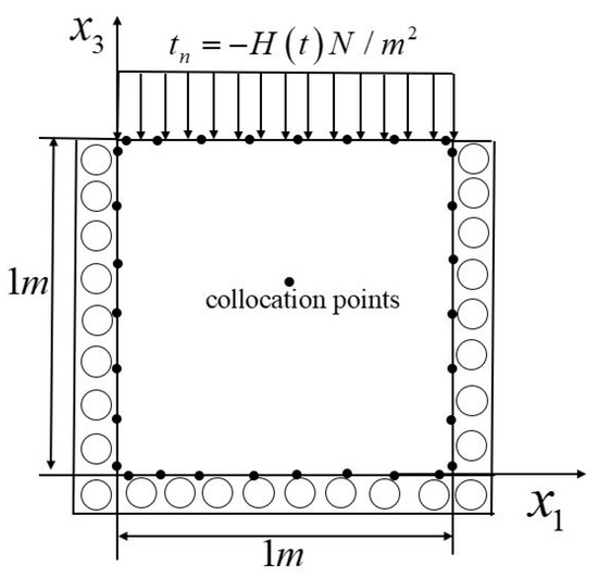
Figure 1. Computational model of saturated column.

Firstly, the transient problem is transformed into the frequency domain. The frequency-domain exact solution for the problem can be constructed as

$$\begin{array}{l}{\tilde{u}}_3^s=a_1\mathrm{j}{k}_1{e}^{\mathrm{j}{k}_1\left(x_3-h\right)}+a_2\mathrm{j}{k}_2{e}^{\mathrm{j}{k}_2\left(x_3-h\right)}-a_3\mathrm{j}{k}_1{e}^{-\mathrm{j}{k}_1{x}_3}-a_4\mathrm{j}{k}_2{e}^{-\mathrm{j}{k}_2{x}_3},\\ \tilde{p}=a_1{r}_1{e}^{\mathrm{j}{k}_1\left(x_3-h\right)}+a_2{r}_2{e}^{\mathrm{j}{k}_2\left(x_3-h\right)}+a_3{r}_1{e}^{-\mathrm{j}{k}_1{x}_3}+a_4{r}_2{e}^{-\mathrm{j}{k}_2{x}_3},\end{array}$$

(37)

in which h = 1 m, and the unknown coefficients $a_1$, $a_2$, $a_3$ and $a_4$ can be derived from

$$\left[\begin{array}{cccc}-k_1^2& -k_2^2& -k_1^2{e}^{-\mathrm{j}{k}_{1}h}& -k_2^2{e}^{-\mathrm{j}{k}_{2}h}\\ r_1& r_2& r_1{e}^{-\mathrm{j}{k}_{1}h}& r_2{e}^{-\mathrm{j}{k}_{2}h}\\ \mathrm{j}{k}_1{e}^{-\mathrm{j}{k}_{1}h}& \mathrm{j}{k}_2{e}^{-\mathrm{j}{k}_{2}h}& -\mathrm{j}{k}_1& -\mathrm{j}{k}_2\\ \mathrm{j}{k}_1\left(r_1-{\omega }^2{\rho }_f\right)e^{-\mathrm{j}{k}_{1}h}& \mathrm{j}{k}_2\left(r_2-{\omega }^2{\rho }_f\right)e^{-\mathrm{j}{k}_{2}h}& \mathrm{j}{k}_1\left(r_1-{\omega }^2{\rho }_f\right)& \mathrm{j}{k}_2\left(r_2-{\omega }^2{\rho }_f\right)\end{array}\right]\left[\begin{array}{l}{a}_1\\ a_2\\ a_3\\ a_4\end{array}\right]=\left[\begin{array}{l}\frac{-1}{\lambda +2\mu }\\ \hspace{0.17em}\hspace{1em}0\\ \hspace{0.17em}\hspace{1em}0\\ \hspace{0.17em}\hspace{1em}0\end{array}\right]$$

Then the transient exact solution is retrieved via the EWM.

The SBM discretizes the boundary into 400 boundary nodes. The EWM-SBM is employed for the numerical solutions in a duration of $T$ = 18 ms. In the EWM, $N_{\omega }$ and $\kappa$ are set as 128 and 3.

In Figure 2, some numerical results are picked up to show the accuracy of the present method, including $u_3^s$ at (0.5, 0.8), $p$ at (0.5, 0.5), $w_3$ at (0.5, 0.7) and ${\sigma }_{33}^s$ at (0.5, 0.3). It is shown that the numerical results are in good agreement with the exact solutions. Nevertheless, the results without the Hanning window function drastically oscillate in the end of the duration, which is called Gibbs oscillations. The problem is ameliorated by the Hanning window function. The application of the Hanning window functions does not bring much time. For example, in Figure 2a, the SBM-EWM without and with the Hanning window functions, respectively, take 57.08 s and 56.48 s. As a consequence, it is essential to employ the window function in the EWM-SBM.

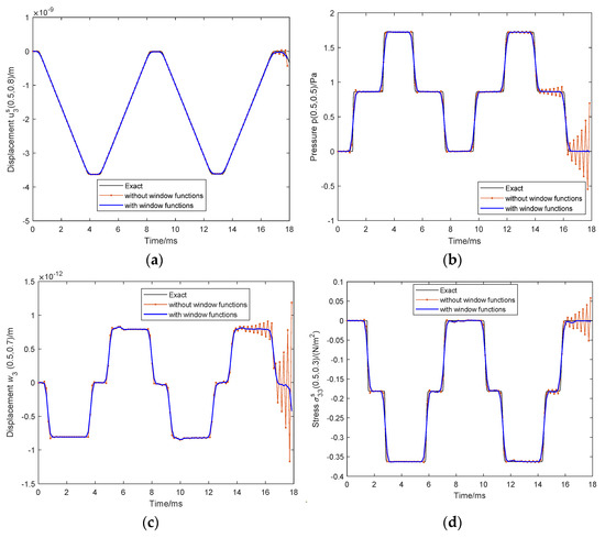
Figure 2. Time history of (a) $u_3^s$ at (0.5, 0.8), (b) p at (0.5, 0.5), (c) $w_3$ at (0.5, 0.7), (d) ${\sigma }_{33}^s$ at (0.5, 0.3).

It is obvious that the selection of the parameters $N_{\omega }$, $\kappa$ has an influence on the accuracy and the stability of the solutions. In the following, the influence is studied.

$N_{\omega }$ is the number of the sample frequencies. More sample frequencies enhance the accuracy of the results but in the meantime bring more operation counts. If the sample frequencies are not enough, the numerical methods may yield inaccurate results. Figure 3 shows the effect of $N_{\omega }$ on the numerical methods via ${\sigma }_{33}^s$ at (0.5, 0.8) and $p$ at (0.5, 0.5). In this figure, the number of boundary points is 400 and $\kappa$ = 2.7. As the number of sampling frequencies increases, the numerical solutions converge to the exact solutions. The solution with $N_{\omega }$ = 64 deviates from the exact solutions most in comparison with $N_{\omega }$ = 128 and 256. However, the case with $N_{\omega }$ = 256 takes 111.7 s in total, which is nearly two times that of the case with $N_{\omega }$ = 128, which consumes 59.3 s. Overall, $N_{\omega }$ = 128 is considered in the following numerical experiments.

Figure 3. Time history of (a) ${\sigma }_{33}^s$ at (0.5, 0.8) and (b) $p$ at (0.5, 0.5) with respect to the number of sampling frequencies $N_{\omega }$.

$\kappa$ is the damping coefficient to determine the artificial damping. A numerical investigation on the $\kappa$ is given in Figure 4 via the absolute error of $u_3^s$ at (0.5, 0.5) under different damping coefficients. $\kappa$ = 1.5, 2, 2.5, 3 and 3.5 are selected. The method with $\kappa$ = 1.5 results in the worst solutions. The reason lies in that more sampling frequencies are required in lightly damped systems. In Figure 4, the results with $\kappa$ = 2, 2.5, 3 and 3.5 are acceptable. Nevertheless, an arbitrary large damping coefficient may lead to loss of numerical precision. As a trade-off, the $\kappa$ = 2.5 is applied in the subsequent examples.

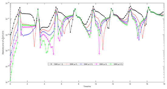
Figure 4. Time history of absolute error of $u_3^s$ at point (0.5, 0.5) under different $\kappa$.

In general, the numerical transient results are limited to a short time duration because the results deteriorate if the calculation duration is too long. In this study, the long time behavior of the present method is investigated. In this case, $T$ = 140 ms and $N_{\omega }$ = 1024. Figure 5 plots the history of $u_3^s$ at (0.5, 0.8) and $p$ at (0.5, 0.5). In the entire calculation time, no obvious differences can be observed between the SBM-EWM and exact solutions, which verifies the accuracy and stability of the SBM-EWM in the long-term dynamic simulation.

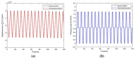
Figure 5. A long time dynamic response of saturated column (a) $u_3^s$ at (0.5, 0.8) and (b) p at (0.5, 0.5).

5.2. A Half-Space Problem Subjected to a Transient Load

In the section, a saturated poroelastic half-space subjected to transient loads on the ground is shown in Figure 6. Thus, the saturated poroelastic half-space is subjected to the boundary condition expressed as

$$\{\begin{array}{l}{t}_3^s=-H\left(t\right)\mathrm{N}/{\mathrm{m}}^2,t_1^s=0\mathrm{N}/{\mathrm{m}}^2,p=0\mathrm{P}\mathrm{a},\hspace{1em}{x}_1\in \left[-1,1\right],x_3=0,\\ t_3^s=0\mathrm{N}/{\mathrm{m}}^2,t_1^s=0\mathrm{N}/{\mathrm{m}}^2,p=0\mathrm{P}\mathrm{a}\hspace{1em}\mathrm{rest}\end{array}$$

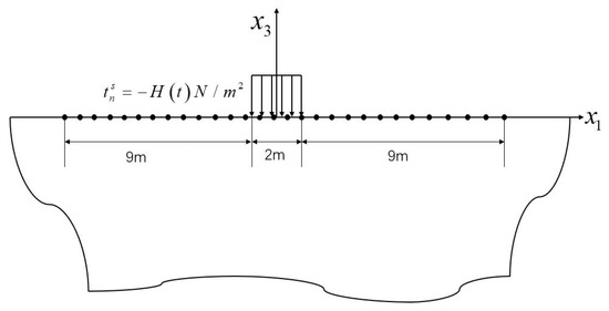
Figure 6. The sketch of the semi-infinite domain.

The boundary is discretized into 500 points. The parameters $N_{\omega }$, $\kappa$ are respectively 128 and 2.5 for the SBM. The analytical solution of this problem in frequency-domain is derived by Ba [59]. Then the transient analytical solution is obtained by the EWM with $N_{\omega }$ = 256 and $\kappa$ = 2.5. The mesh plots of the analytical solutions and SBM solutions are displayed in Figure 7 and Figure 8. The solutions at different times at different depths are plotted. Good agreement indicates that the SBM is successfully applied to the half-space transient problem.

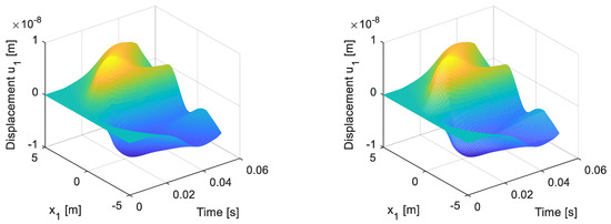
Figure 7. Time history of u₁ at x₃ = −1 generated by the analytical solution (left) and the SBM-EWM (right).

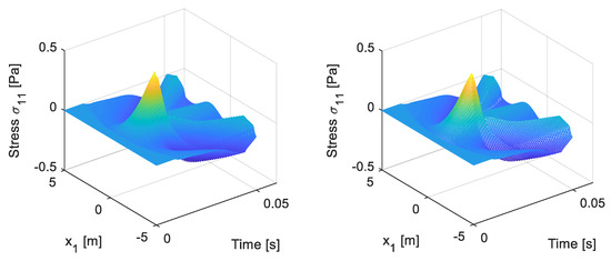
Figure 8. Time history of σ₁₁ at x₃ = −2 generated by the analytical solution (left) and the SBM-EWM (right).

Furthermore, the MFS is introduced for comparison with the SBM in Figure 9. All the parameters for the MFS and SBM are the same as the above. The MFS avoids the origin singularity via the artificial boundary outside the computational domain. d is the distance between the artificial boundary and physical boundary. To obtain stable solutions, the MATLAB built-in function pinv is used to solve the linear system of the MFS. As shown in the figure, the MFS and SBM could obtain acceptable solutions. Nevertheless, the results of the MFS are influenced by the location of the artificial boundary. Only the MFS with d = 0.1 converges to the analytical solutions. Otherwise, because of the application of pinv, the MFS takes 357.34 s for the whole process, while the SBM takes 92.96 s. It can be observed that the MFS takes a much longer time than the SBM.

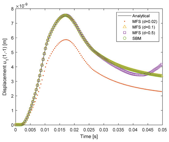
Figure 9. Numerical comparison between the MFS and SBM.

5.3. A Tunnel Embedded in a Saturated Poroelastic Half-Space

In this example, a model of a semi-circular tunnel embedded in a saturated poroelastic half-space in Figure 10 is considered. The radius of the tunnel is R = 3 m and the depth of invert of the tunnel is H = 6 m. A triangularly distributed transient load is imposed at the invert of the tunnel. The ground and the surface of the tunnel are set as permeable. Thus, the boundary conditions are expressed as

$$\{\begin{array}{l}{t}_3^s=\left(\left(\left|x\right|-3\right)P\left(t\right)\right){\mathrm{N}/\mathrm{m}}^2, t_1^s=0{\mathrm{N}/\mathrm{m}}^2,p=0\mathrm{P}\mathrm{a},\hspace{1em}{x}_1\in \left[-3, 3\right], x_3=-6\\ t_3^s=0\mathrm{N}/{\mathrm{m}}^2,t_1^s=0\mathrm{N}/{\mathrm{m}}^2,p=0\mathrm{P}\mathrm{a},\hspace{1em}\mathrm{otherwise}\end{array},$$

where

$$P\left(t\right)=\{\begin{array}{l}100t\hspace{1em}0\le t\le 0.01\\ 1\hspace{1em}\hspace{1em}0.01<t\le 0.03\\ 4-100t\hspace{1em}0.03<t\le 0.04\\ 0\hspace{1em}\mathrm{otherwise}\end{array}$$

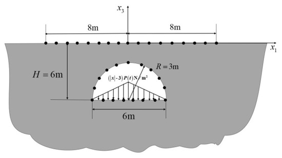
Figure 10. Schematic sketch of the semi-infinite domain tunnel.

In this case, no analytical solution is available. Thus, the accuracy of the SBM-EWM is presented with different parameters. The total time of tunnel transient response T is 90 ms, and the damping coefficient $\mathit{\kappa }$ is 2.5. Figure 11 gives ${\sigma }_{33}^s$ at (−2, −7) and $p$ at (1, −7) calculated by the SBM-EWM with different numbers of sampling frequencies $N_{\omega }$ (128, 256) and numbers of boundary points N (471, 786). It is observed that the SBM-EWM with different parameters obtains identical results.

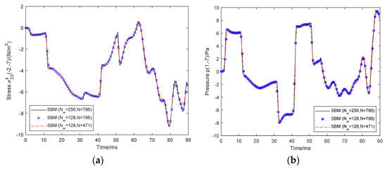
Figure 11. Time history of (a) ${\sigma }_{33}^s$ at (−2, −7) and (b) p at (1, −7) under different sampling numbers and boundary points.

To further investigate the numerical results, the time history of the distribution of $u_3^s$ and p of the domain $(x_1,x_3)\in \left[-10,\hspace{0.17em}10\right]\times \left[-20,\hspace{0.17em}0\right]$ are plotted in Figure 12 and Figure 13 to observe the wave propagation in the entire time. In all results, the dynamic response is symmetric, which is reasonable according to the symmetry loads. In both figures, it can be seen that the wave is caused by loads at the invert of the tunnel. Then it propagates outward in different directions and around the tunnel to the ground. Theoretically speaking, the whole propagation process complies with the law of wave propagation in solids.

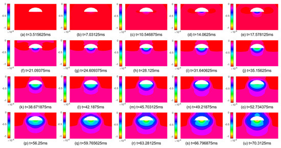
Figure 12. Distribution of $u_3^s$ with of domain $(x_1,x_3)\in \left[-10,\hspace{0.17em}10\right]\times \left[-20,\hspace{0.17em}0\right]$ at different times.

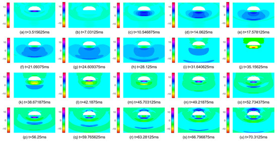
Figure 13. Distribution of p with of domain $(x_1,x_3)\in \left[-10,\hspace{0.17em}10\right]\times \left[-20,\hspace{0.17em}0\right]$ at different times.

6. Conclusions

In this paper, a novel boundary-only meshless approach is developed to simulate transient dynamic response in the saturated soil. In this method, the SBM is employed to solve the frequency-domain governing equations, while the EWM transforms the frequency-domain solutions into time-domain solutions. In the SBM, the solutions are approximated via the fundamental solutions in terms of boundary points. The boundary-only property makes the SBM very suitable in solving semi-infinite domain problems. The fundamental solutions are derived via the wave decomposition method and eigenanalysis, and their source singularities are removed by the OIFs. The EWM is boasted as an effective inverse Fourier transform method, which incorporates exponential artificial damping into the FFT to enhance its numerical efficiency. The Hanning window function is used to smooth the Gibbs oscillation as the computation period increases. The influence of the parameters in the EWM was investigated in the first numerical experiment. All numerical results validate that the present SBM-EWM is accurate and effective to solve the transient soil dynamic response. Nevertheless, the SBM-EWM is only applicable when the fundamental solutions exist because the fundamental solutions are the kernel function of the SBM.

References

- Chen, G.; Yang, J.; Liu, Y.; Kitahara, T.; Beer, M. An energy-frequency parameter for earthquake ground motion intensity measure. Earthq. Eng. Struct. Dyn. 2022, 1–14. [Google Scholar] [CrossRef]
- Chen, G.; Li, Q.-Y.; Li, D.-Q.; Wu, Z.-Y.; Liu, Y. Main frequency band of blast vibration signal based on wavelet packet transform. Appl. Math. Model. 2019, 74, 569–585. [Google Scholar] [CrossRef]
- Li, W.; Zhang, Q.; Gui, Q.; Chai, Y. A Coupled FE-Meshfree Triangular Element for Acoustic Radiation Problems. Int. J. Comput. Methods 2021, 18, 2041002. [Google Scholar] [CrossRef]
- Chai, Y.; Li, W.; Liu, Z. Analysis of transient wave propagation dynamics using the enriched finite element method with interpolation cover functions. Appl. Math. Comput. 2022, 412, 126564. [Google Scholar] [CrossRef]
- Pled, F.; Desceliers, C. Review and Recent Developments on the Perfectly Matched Layer (PML) Method for the Numerical Modeling and Simulation of Elastic Wave Propagation in Unbounded Domains. Arch. Comput. Methods Eng. 2022, 29, 471–518. [Google Scholar] [CrossRef]
- Fu, Z.-J.; Xie, Z.-Y.; Ji, S.-Y.; Tsai, C.-C.; Li, A.-L. Meshless generalized finite difference method for water wave interactions with multiple-bottom-seated-cylinder-array structures. Ocean Eng. 2020, 195, 106736. [Google Scholar] [CrossRef]
- Kythe, P.K. Fundamental Solutions for Differential Operators and Applications; Birkhauser: Basel, Switzerland, 1996. [Google Scholar]
- Chen, C.S.; Karageorghis, A.; Smyrlis, Y.S. The Method of Fundamental Solutions: A Meshless Method; Dynamic Publishers: Atlanta, GA, USA, 2008. [Google Scholar]
- Wei, X.; Chen, W.; Chen, B. An ACA accelerated MFS for potential problems. Eng. Anal. Bound. Elem. 2014, 41, 90–97. [Google Scholar] [CrossRef]
- Chen, Z.; Sun, L. A boundary meshless method for dynamic coupled thermoelasticity problems. Appl. Math. Lett. 2022, 134, 108305. [Google Scholar] [CrossRef]
- Wang, M.Z.; Xu, B.X.; Gao, C.F. Recent General Solutions in Linear Elasticity and Their Applications. Appl. Mech. Rev. 2008, 61, 030803–030820. [Google Scholar] [CrossRef]
- Sun, L.; Zhang, C.; Yu, Y. A boundary knot method for 3D time harmonic elastic wave problems. Appl. Math. Lett. 2020, 104, 106210. [Google Scholar] [CrossRef]
- Xu, W.-Z.; Fu, Z.-J.; Xi, Q. A novel localized collocation solver based on a radial Trefftz basis for thermal conduction analysis in FGMs with exponential variations. Comput. Math. Appl. 2022, 117, 24–38. [Google Scholar] [CrossRef]
- Xi, Q.; Fu, Z.; Zhang, C.; Yin, D. An efficient localized Trefftz-based collocation scheme for heat conduction analysis in two kinds of heterogeneous materials under temperature loading. Comput. Struct. 2021, 255, 106619. [Google Scholar] [CrossRef]
- Li, Z.C.; Lu, T.T.; Hu, H.Y.; Cheng, A.H.D. Trefftz and Collocation Methods; WIT Press: Boston, UK, 2008. [Google Scholar]
- Sun, L.; Wei, X.; Chu, L. A 2D frequency-domain wave based method for dynamic analysis of orthotropic solids. Comput. Struct. 2020, 238, 106300. [Google Scholar] [CrossRef]
- Karageorghis, A.; Lesnic, D.; Marin, L. A survey of applications of the MFS to inverse problems. Inverse Probl. Sci. Eng. 2011, 19, 309–336. [Google Scholar] [CrossRef]
- Šarler, B. Solution of potential flow problems by the modified method of fundamental solutions: Formulations with the single layer and the double layer fundamental solutions. Eng. Anal. Bound. Elem. 2009, 33, 1374–1382. [Google Scholar] [CrossRef]
- Chen, W. Singular boundary method: A novel, simple, meshfree, boundary collocation numerical method. Chin. J. Solid Mech. 2009, 30, 592–599. [Google Scholar]
- Wei, X.; Chen, W.; Chen, B.; Sun, L. Singular boundary method for heat conduction problems with certain spatially varying conductivity. Comput. Math. Appl. 2015, 69, 206–222. [Google Scholar] [CrossRef]
- Wei, X.; Chen, W.; Sun, L.; Chen, B. A simple accurate formula evaluating origin intensity factor in singular boundary method for two-dimensional potential problems with Dirichlet boundary. Eng. Anal. Bound. Elem. 2015, 58, 151–165. [Google Scholar] [CrossRef]
- Wei, X.; Chen, W.; Fu, Z.J. Solving inhomogeneous problems by singular boundary method. J. Mar. Sci. Technol. Taiwan 2013, 21, 8–14. [Google Scholar] [CrossRef]
- Wei, X.; Sun, L.; Yin, S.; Chen, B. A boundary-only treatment by singular boundary method for two-dimensional inhomogeneous problems. Appl. Math. Model. 2018, 62, 338–351. [Google Scholar] [CrossRef]
- Wei, X.; Sun, L. Singular boundary method for 3D time-harmonic electromagnetic scattering problems. Appl. Math. Model. 2019, 76, 617–631. [Google Scholar] [CrossRef]
- Wei, X.; Huang, A.; Sun, L. Singular boundary method for 2D and 3D heat source reconstruction. Appl. Math. Lett. 2020, 102, 106103. [Google Scholar] [CrossRef]
- Wei, X.; Luo, W. 2.5D singular boundary method for acoustic wave propagation. Appl. Math. Lett. 2021, 112, 106760. [Google Scholar] [CrossRef]
- Cheng, S.; Wang, F.; Li, P.-W.; Qu, W. Singular boundary method for 2D and 3D acoustic design sensitivity analysis. Comput. Math. Appl. 2022, 119, 371–386. [Google Scholar] [CrossRef]
- Fu, Z.; Xi, Q.; Li, Y.; Huang, H.; Rabczuk, T. Hybrid FEM–SBM solver for structural vibration induced underwater acoustic radiation in shallow marine environment. Comput. Methods Appl. Mech. Eng. 2020, 369, 113236. [Google Scholar] [CrossRef]
- Wei, X.; Rao, C.; Chen, S.; Luo, W. Numerical simulation of anti-plane wave propagation in heterogeneous media. Appl. Math. Lett. 2023, 135, 108436. [Google Scholar] [CrossRef]
- Sun, L.; Wei, X. A frequency domain formulation of the singular boundary method for dynamic analysis of thin elastic plate. Eng. Anal. Bound. Elem. 2019, 98, 77–87. [Google Scholar] [CrossRef]
- Sun, L.; Chen, W.; Cheng, A.H.D. Singular boundary method for 2D dynamic poroelastic problems. Wave Motion 2016, 61, 40–62. [Google Scholar] [CrossRef]
- Sun, L.; Wei, X.; Chen, B. A meshless singular boundary method for elastic wave propagation in 2D partially saturated poroelastic media. Eng. Anal. Bound. Elem. 2020, 113, 82–98. [Google Scholar] [CrossRef]
- Li, W.; Wang, F. Precorrected-FFT Accelerated Singular Boundary Method for High-Frequency Acoustic Radiation and Scattering. Mathematics 2022, 10, 238. [Google Scholar] [CrossRef]
- Li, J.; Gu, Y.; Qin, Q.-H.; Zhang, L. The rapid assessment for three-dimensional potential model of large-scale particle system by a modified multilevel fast multipole algorithm. Comput. Math. Appl. 2021, 89, 127–138. [Google Scholar] [CrossRef]
- Li, J.; Zhang, L.; Qin, Q. A regularized fast multipole method of moments for rapid calculation of three-dimensional time-harmonic electromagnetic scattering from complex targets. Eng. Anal. Bound. Elem. 2022, 142, 28–38. [Google Scholar] [CrossRef]
- Li, J.; Fu, Z.; Gu, Y.; Qin, Q. Recent advances and emerging applications of the singular boundary method for large-scale and high-frequency computational acoustics. Adv. Appl. Math. Mech. 2022, 14, 315–343. [Google Scholar] [CrossRef]
- Qu, W.; Chen, W.; Zheng, C. Diagonal form fast multipole singular boundary method applied to the solution of high-frequency acoustic radiation and scattering. Int. J. Numer. Methods Eng. 2017, 111, 803–815. [Google Scholar] [CrossRef]
- Fu, Z.; Tang, Z.; Xi, Q.; Liu, Q.; Gu, Y.; Wang, F. Localized collocation schemes and their applications. Acta Mech. Sin. 2022, 38, 422167. [Google Scholar] [CrossRef]
- Li, W. Localized method of fundamental solutions for 2D harmonic elastic wave problems. Appl. Math. Lett. 2021, 112, 106759. [Google Scholar] [CrossRef]
- Zhu, T.; Zhang, J.D.; Atluri, S.N. A local boundary integral equation (LBIE) method in Comput. Mech., and a meshless discretization approach. Comput. Mech. 1998, 21, 223–235. [Google Scholar] [CrossRef]
- Sun, L.; Fu, Z.; Chen, Z. A localized collocation solver based on fundamental solutions for 3D time harmonic elastic wave propagation analysis. Appl. Math. Comput. 2023, 439, 127600. [Google Scholar] [CrossRef]
- Zhang, Y.; Dang, S.; Li, W.; Chai, Y. Performance of the radial point interpolation method (RPIM) with implicit time integration scheme for transient wave propagation dynamics. Comput. Math. Appl. 2022, 114, 95–111. [Google Scholar] [CrossRef]
- Qu, W.; He, H. A spatial–temporal GFDM with an additional condition for transient heat conduction analysis of FGMs. Appl. Math. Lett. 2020, 110, 106579. [Google Scholar] [CrossRef]
- Gao, X.-W.; Zheng, B.-J.; Yang, K.; Zhang, C. Radial integration BEM for dynamic coupled thermoelastic analysis under thermal shock loading. Comput. Struct. 2015, 158, 140–147. [Google Scholar] [CrossRef]
- Kuhlman, K. Review of inverse Laplace transform algorithms for Laplace-space numerical approaches. Numer. Algorithms 2013, 63, 339–355. [Google Scholar] [CrossRef]
- Xiao, J.; Ye, W.; Cai, Y.; Zhang, J. Precorrected FFT accelerated BEM for large-scale transient elastodynamic analysis using frequency-domain approach. Int. J. Numer. Methods Eng. 2012, 90, 116–134. [Google Scholar] [CrossRef]
- Phan, A.V.; Gray, L.J.; Salvadori, A. Transient analysis of the dynamic stress intensity factors using SGBEM for frequency-domain elastodynamics. Comput. Methods Appl. Mech. Eng. 2010, 199, 3039–3050. [Google Scholar] [CrossRef]
- Marrero, M.; Domínguez, J. Numerical behavior of time domain BEM for three-dimensional transient elastodynamic problems. Eng. Anal. Bound. Elem. 2003, 27, 39–48. [Google Scholar] [CrossRef]
- Qu, W.; Gao, H.W.; Gu, Y. Integrating Krylov deferred correction and generalized finite difference methods for dynamic simulations of wave propagation phenomena in long-time intervals. Adv. Appl. Math. Mech. 2021, 13, 1398–1417. [Google Scholar]
- Kausel, E.; Roësset, J.M. Frequency Domain Analysis of Undamped Systems. J. Eng. Mech. 1992, 118, 721–734. [Google Scholar] [CrossRef]
- Tong, L.H.; Ding, H.B.; Yan, J.W.; Xu, C.; Lei, Z. Strain gradient nonlocal Biot poromechanics. Int. J. Eng. Sci. 2020, 156, 103372. [Google Scholar] [CrossRef]
- Tong, L.; Yu, Y.; Hu, W.; Shi, Y.; Xu, C. On wave propagation characteristics in fluid saturated porous materials by a nonlocal Biot theory. J. Sound Vib. 2016, 379, 106–118. [Google Scholar] [CrossRef]
- Biot, M.A. Theory of Propagation of Elastic Waves in a Fluid-Saturated Porous Solid. II. Higher Frequency Range. J. Acoust. Soc. Am. 1956, 28, 179–191. [Google Scholar] [CrossRef]
- Lu, J.F.; Jeng, D.S.; Williams, S. A 2.5-D dynamic model for a saturated porous medium: Part I. Green’s function. Int. J. Solids Struct. 2008, 45, 378–391. [Google Scholar] [CrossRef]
- Wei, X.; Liu, D.; Luo, W.; Chen, S.; Sun, L. A half-space singular boundary method for predicting ground-borne vibrations. Appl. Math. Model. 2022, 111, 630–643. [Google Scholar] [CrossRef]
- Gu, Y.; Chen, W.; Zhang, C.-Z. Singular boundary method for solving plane strain elastostatic problems. Int. J. Solids Struct. 2011, 48, 2549–2556. [Google Scholar] [CrossRef]
- Ariza, M.P.; Dominguez, J. General BE approach for three-dimensional dynamic fracture analysis. Eng. Anal. Bound. Elem. 2002, 26, 639–651. [Google Scholar] [CrossRef]
- Xiao, J.; Ye, W.; Wen, L. Efficiency improvement of the frequency-domain BEM for rapid transient elastodynamic analysis. Comput. Mech. 2013, 52, 903–912. [Google Scholar] [CrossRef]
- Ba, Z.; Kang, Z.; Lee, V.W. Plane strain dynamic responses of a multi-layered transversely isotropic saturated half-space. Int. J. Eng. Sci. 2017, 119, 55–77. [Google Scholar] [CrossRef]
Publisher’s Note: MDPI stays neutral with regard to jurisdictional claims in published maps and institutional affiliations. |
© 2022 by the authors. Licensee MDPI, Basel, Switzerland. This article is an open access article distributed under the terms and conditions of the Creative Commons Attribution (CC BY) license (https://creativecommons.org/licenses/by/4.0/).