Alternative Method to Estimate the Fourier Expansions and Its Rate of Change

Abstract

This paper presents a methodology to obtain the Fourier coefficients (FCs) and the derivative Fourier coefficients (DFCs) from an input signal. Based on the Taylor series that approximates the input signal into a trigonometric signal model through the Kalman filter, consequently, the signal’s and successive derivatives’ coefficients are obtained with the state prediction and the state matrix inverse. Compared to discrete Fourier transform (DFT), the new class of filters provides noise reduction and sidelobe suppression advantages. Additionally, the proposed Taylor–Kalman–Fourier algorithm (TKFA) achieves a null-flat frequency response around the frequency operation. Moreover, with the proposed TKFA method, the decrement in the inter-harmonic amplitude is more significant than that obtained with the Kalman–Fourier algorithm (KFA), and the neighborhood of the null-flat frequency is expanded. Finally, the approximation of the input signal and its derivative can be performed with a sum of functions related to the estimated coefficients and their respective harmonics.

1. Introduction

Signal analysis is implemented in many areas because it allows for obtaining characteristics or relevant information about systems. It has been employed in different areas, such as power systems, vibration analysis, speech recognition, energy processing, radar applications, time series modeling, biomedical engineering, and digital communications. For instance, [1] gave the generalized sampling expansions (GSE) in the realm of a one-dimensional quaternion Fourier transform. Ref. [2] employed the Fourier coefficients (FCs) to fit the GPS precise ephemeris. In [3,4], the Fourier series coefficients were used in a tracking control trajectory. In the both of the last cases, obtaining more information could help better control GPS and tracking control, not only regarding the trajectory, but also its speed.

The most commonly used tool to obtain information about systems is the Fourier transform. In the literature, it is possible to find some strategies to obtain better precision in the estimation of the FCs in different conditions. In [5], the discrete Fourier transform (DFT) is used to estimate the periodic signal’s FCs. On the other hand, the impact of the data windows in the estimation of FCs was analyzed by [6]. The recursive discrete Fourier transform (RDFT) [7,8,9] is another strategy that considers a structure of the DFT with a multi-rate sampling. One disadvantage of the last method is that it takes a sinusoidal signal as a model. Therefore, the estimates can be downgraded when the input is different from the sinusoidal signal, for example, a quasi-periodic signal. Another disadvantage is that obtained estimates provided a delay due to the implemented windows in the algorithms. To solve the first disadvantage, when the measurement signal does not satisfy the ideal conditions (when the input signal is not sinusoidal), this occurs when the measurement signal is quasi-periodic. In [10,11], the authors implemented a quasi-periodic signal model considering an optimal FIR filter, whereas in [12], the authors improved the approximation of a sufficiently smooth nonperiodic function defined on a compact interval by proposing alternative forms of Fourier series expansions. In [13], an algorithm was proposed that was derived from the least mean squares (LMS) that can estimate the FCs of a sinusoidal and quasi-periodic signal. Then, to solve the delay problem in the estimates, in [14,15], the FCs were obtained with a Kalman filter.

Systems can be modified through time by different circumstances. For example, the evolution in the systems can be due to wear or operation conditions. For this reason, is not enough to estimate the FCs. The derivative of the Fourier coefficients (DFCs) provides information on the evolution of systems over time. In this work, the FCs are estimated without delay because the estimations are achieved with a quasi-periodic dynamic signal model applied to the Kalman filter. Additionally, at the same time, the DFCs are estimated. With the Taylor polynomial approximation to the signal model and its derivatives, it can develop a state space model, where the first row in the state matrix is the approximation to the signal model, the second is the approximation to the first derivative, and so on. Thereby, with the state space model implemented in the Kalman filter, it is possible to obtain the FC and DFC estimates in synchronous time. Additionally, the harmonics and their derivatives can be estimated with an extension of the state matrix with its harmonics. Recently, some techniques have been proposed to estimate the FCs. Ref. [16] determined the coefficient in the representation of two polynomials as a linear combination of an arbitrary polynomial sequence to achieve the above derivative of the Fourier series. Ref. [17] considered unbiased Fourier coefficients for reducing systematics in applications of large cosmological data sets in grid size. In [18], the authors proposed an algorithm for the identification of significant frequencies and the estimation of the Fourier coefficients. However, they did not estimate the DFCs. In [19], the authors employed the Fourier cosine series expansion (COS) to value the guaranteed minimum death benefit products.

The aim of the proposed method is based on two stages. In the first stage, with the Taylor polynomial implemented in the Kalman filter, the signal and its derivatives are estimates. In the second stage, the coefficients and their derivatives are calculated by considering the estimations obtained from the Kalman filter and the state-proposed matrix. Here we observe that when a zero-order Taylor polynomial is employed as an analytic function in the Kalman filter, the results are equivalent to the traditional Fourier series. With the expansion of the Taylor polynomial with an order greater than zero, the estimation results of the Fourier coefficients are improved. Moreover, it can be confirmed in the magnitude response of the proposed method, where the magnitude in harmonic frequencies is flat.

The remainder of this paper is organized as follows. First, the state space observer approach is described in Section 2. The Kalman filter applied and the structure implemented to obtain the coefficients are illustrated in Section 3. The performance of the proposed method is shown in Section 4. A summary of our conclusions closes the paper in Section 5.

2. The Spectral Observer Approach

It is common to implement the Fourier series as a signal model [20,21] that is defined as follows

$$\begin{array}{c}\hfill z_k=a_k^0+\sum _{\ell =1}^N\left(a_k^{\ell }cos\left(\frac{\ell 2\pi k}{2N+1}\right)+b_k^{\ell }sin\left(\frac{\ell 2\pi k}{2N+1}\right)\right),\end{array}$$

(1)

where the number of samples per period T is $2N+1$, and ℓ represent the harmonic components. However, here, we propose a quasi-periodic signal inspired by (1). In its first stage, it is approximate around $t_0$ by a M-th order Taylor polynomial as

$${\zeta }_k=\sum _{m=0}^M\frac{f{\left(\frac{2\pi k}{N_1}\right)}^{\left(m\right)}}{m!}{\tau }^{\left(m\right)},$$

(2)

with $t_0=[n-1]\tau$ at time $t=n\tau$, and $\tau =t-t_0$. The function $f(·)$ in (2) is defined as

$$f\left(\frac{2\pi k}{N_1}\right)=cos\left(\frac{2\pi k}{N_1}\right)+sin\left(\frac{2\pi k}{N_1}\right).$$

(3)

Hence, the real part of the function in (2) is denoted as

$${\mathsf{\Delta }}_{r,k}=\sum _{m=0}^M\frac{{\left(a_{m}cos\left(\frac{2\pi k}{N_1}\right)\right)}^{\left(m\right)}}{m!}{\tau }^{\left(m\right)},$$

(4)

and the imaginary part is

$${\mathsf{\Delta }}_{i,k}=\sum _{m=0}^M\frac{{\left(b_{m}sin\left(\frac{2\pi k}{N_1}\right)\right)}^{\left(m\right)}}{m!}{\tau }^{\left(m\right)},$$

(5)

where $N_1$ is the number of samples per cycle in the input signal, and M is the order of the polynomial approximation.

With (4) and its successive derivatives, the following matrix is obtained:

$${\mathsf{\Lambda }}_r=\left[\begin{array}{cccc}{\alpha }_{1,1}& {\alpha }_{1,2}& \dots & {\alpha }_{1,m}\\ {\alpha }_{2,1}& {\alpha }_{2,2}& \dots & {\alpha }_{2,m}\\ ⋮& ⋮& ⋮& ⋮\\ {\alpha }_{m,1}& {\alpha }_{m,2}& \dots & {\alpha }_{m,m}\end{array}\right]cos\left(\omega \tau \right),$$

(6)

where the coefficients ${\alpha }_{i,j}$ with, $i=1,\dots ,m$ and $j=1,\dots ,m$ are given as follows:

${\alpha }_{1,1}=1$,	${\alpha }_{1,2}=\tau$,	${\alpha }_{1,m}=\frac{{\tau }^m}{m!}$;
${\alpha }_{2,1}=j\omega$,	${\alpha }_{2,2}=(j\omega \tau +1)$,	${\alpha }_{2,m}=j\omega \frac{{\tau }^m}{m!}+\frac{{\tau }^{m-1}}{(m-1)!}$;
${\alpha }_{m,1}={\left(j\omega \right)}^m$;
${\alpha }_{m,2}={\left(j\omega \right)}^m\tau +m{\left(j\omega \right)}^{m-1}$;
${\alpha }_{m,m}={\left(j\omega \right)}^m\frac{{\tau }^m}{m!}+m{\left(j\omega \right)}^{m-1}\frac{{\tau }^{m-1}}{(K-1)!}+\dots +1$;

with $\omega =\frac{2\pi }{N_1}$ and $\tau =\frac{1}{N_1}$. On the other hand, the imaginary part (5) and its derivatives can be represented as

$${\mathsf{\Lambda }}_i=j\left[\begin{array}{cccc}{\alpha }_{1,1}& {\alpha }_{1,2}& \dots & {\alpha }_{1,m}\\ {\alpha }_{2,1}& {\alpha }_{2,2}& \dots & {\alpha }_{2,m}\\ ⋮& ⋮& ⋮& ⋮\\ {\alpha }_{m,1}& {\alpha }_{m,2}& \dots & {\alpha }_{m,m}\end{array}\right]sin\left(\omega \tau \right).$$

(7)

Then, the signal model defined by (2) and its derivative is given as

$$\left[\begin{array}{c}{\zeta }_k\\ {\overline{\zeta }}_k\end{array}\right]=\left[\begin{array}{cc}{\mathsf{\Lambda }}_r& {\mathsf{\Lambda }}_i\\ -{\mathsf{\Lambda }}_i& {\mathsf{\Lambda }}_r\end{array}\right]\left[\begin{array}{c}a\\ b\end{array}\right],$$

(8)

where ${\overline{\zeta }}_k$ is the complex conjugate of ${\zeta }_k$. Therefore,

$$\left[\begin{array}{c}a\\ b\end{array}\right]={\left[\begin{array}{cc}{\mathsf{\Lambda }}_r& {\mathsf{\Lambda }}_i\\ -{\mathsf{\Lambda }}_i& {\mathsf{\Lambda }}_r\end{array}\right]}^{-1}\left[\begin{array}{c}{\zeta }_k\\ {\overline{\zeta }}_k\end{array}\right].$$

(9)

Note that $a={[a{a}_1{a}_2\dots a_m]}^T$, $b={[b{b}_1{b}_2\dots b_m]}^T$, and ${\zeta }_{k,\ell }=[{\zeta }_k{\dot{\zeta }}_k{\ddot{\zeta }}_k\dots$ ${\zeta }_k^{\left(m\right)}]$. As the coefficients a and b correspond to $\zeta ={[{\zeta }_k,\overline{{\zeta }_k}]}^T$, consequently, the coefficients $a_1$ and $b_1$ correspond to $\dot{{\zeta }_k}$; therefore, its coefficients are called DFCs.

In the next section, the state transition matrix is extended to all sets of harmonics and is implemented to extract the coefficients.

3. The Kalman Filter Applied and Coefficient Estimates

This section illustrates the construction of the signal model and its implementation in the Kalman filter, where two methodologies are considered. The first method is when the signal model is approximate with a zero-order Taylor polynomial defined in (2). The second method is obtained when the signal model is approximate with a higher-than-zero-order.

3.1. Kalman Filter Algorithm (KFA)

With the matrix (6) and (14), we developed a signal model, as can be seen in (8), that is implemented in the Kalman filter. Ehen the order of the signal model is defined as $m=1$ and $l=1$, the algorithm is called a Kalman filter algorithm (KFA). Thus, the state prediction and the measurement equation are defined as.

$$x_{k+1}=\mathsf{\Psi }{x}_k+G{w}_k,$$

(10a)

$${\zeta }_k=H{x}_{k+1},$$

(10b)

where

$$\begin{array}{c}\hfill \mathsf{\Psi }=\left[\begin{array}{cc}{\mathsf{\Lambda }}_{r,\ell }& {\mathsf{\Lambda }}_{i,\ell }\\ -{\mathsf{\Lambda }}_{i,\ell }& {\mathsf{\Lambda }}_{r,\ell }\end{array}\right]\end{array}$$

(11)

$$h=[10,\dots ,0]\in {\Re }^{\left(2\right(K+1\left)\right)},$$

(12)

3.2. Taylor–Kalman–Fourier Algorithm (TKFA)

The matrix (15) can be expanded with the ℓ array of ${\mathsf{\Delta }}_r$ and ${\mathsf{\Delta }}_i$, where the functions $cos$ and $sin$ have the respective ℓ harmonics as

$${\mathsf{\Lambda }}_{r,\ell }=\left[\begin{array}{cccc}{\alpha }_{1,1}& {\alpha }_{1,2}& \dots & {\alpha }_{1,m}\\ {\alpha }_{2,1}& {\alpha }_{2,2}& \dots & {\alpha }_{2,m}\\ ⋮& ⋮& ⋮& ⋮\\ {\alpha }_{m,1}& {\alpha }_{m,2}& \dots & {\alpha }_{m,m}\end{array}\right]cos(\ell \omega \tau ).$$

(13)

and

$${\mathsf{\Lambda }}_{i,\ell }=j\left[\begin{array}{cccc}{\alpha }_{1,1}& {\alpha }_{1,2}& \dots & {\alpha }_{1,m}\\ {\alpha }_{2,1}& {\alpha }_{2,2}& \dots & {\alpha }_{2,m}\\ ⋮& ⋮& ⋮& ⋮\\ {\alpha }_{m,1}& {\alpha }_{m,2}& \dots & {\alpha }_{m,m}\end{array}\right]sin(\ell \omega \tau ).$$

(14)

with $\ell =1,\dots ,N$.

On the other hand, when the transition matrix is expanded with $\ell >1$, and the approximation to the model signal is greater than one ($m>1$), the filter is named a Taylor–Kalman–Fourier algorithm (TKFA), and the state transition matrix and the measurement equation are defined as

$$\begin{array}{c}\hfill \mathsf{\Psi }=\left\{\mathrm{B}\mathrm{l}\mathrm{o}\mathrm{c}\mathrm{k}\mathrm{d}\mathrm{i}\mathrm{a}\mathrm{g}\left[\begin{array}{cc}{\mathsf{\Lambda }}_{r,\ell }& {\mathsf{\Lambda }}_{i,\ell }\\ -{\mathsf{\Lambda }}_{i,\ell }& {\mathsf{\Lambda }}_{r,\ell }\end{array}\right];\ell =1,\dots ,N\right.\},\end{array}$$

(15)

$$H=[hh,\dots ,h]\in {\Re }^{N\left(2\right(K+1\left)\right)},$$

(16)

Remark 1.

When the parameters m and ℓ of matrix Ψ in (15) are set as $m=1$ and $\ell =1$, then the algorithm is called a KFA.

With the discrete state space model (10a) and the truncated discrete signal model (10b), the standard discrete Kalman filter [22,23] is applied to obtain the state estimation ${\widehat{x}}_{k+1}$ according to Algorithm 1.

Algorithm 1 Pseudocode of the Kalman filter algorithm.

1: procedure

2:       –Inputs

3:       $s\left[n\right]\leftarrow$ Input current signal for $n=1$ up to $(2N+1)$,

4:       $\widehat{\mathit{x}}[n-1]\leftarrow$ Guess initial internal variables,

5:       $\widehat{\omega }\left[0\right]\leftarrow$ Guess initial frequency,

6:       $\mathit{P}[n-1]\leftarrow$ Guess initial covariance,

7:       ${\sigma }_v^2\leftarrow$ Variance of process noise,

8:       ${\sigma }_w^2\leftarrow$ Variance of measurement noise,

9:       $\mathsf{\Psi },H\leftarrow$ Signal model parameters,

10:       for $n=1$ to $(2N+1)$ do

11:            –State prediction

12:            ${\widehat{\mathit{x}}}^{-}\left[n\right]\leftarrow \mathsf{\Psi }\widehat{\mathit{x}}[n-1]$,

13:            ${\mathit{P}}^{-}\left[n\right]\leftarrow \mathsf{\Psi }\mathit{P}[n-1]{\left(\mathsf{\Psi }\right)}^H+\mathsf{\Gamma }{\mathsf{\Gamma }}^H{\sigma }_v^2$,

14:            –Measurement update

15:            $\mathit{K}\left[n\right]\leftarrow {\mathit{P}}^{-}\left[n\right]{\mathit{H}}^T{(\mathit{H}{\mathit{P}}^{-}\left[n\right]{\mathit{H}}^T+{\sigma }_w^2)}^{-1}$,

16:            $\widehat{\mathit{x}}\left[n\right]\leftarrow {\widehat{\mathit{x}}}^{-}\left[n\right]+\mathit{K}\left[n\right](s\left[n\right]-\mathit{H}{\widehat{\mathit{x}}}^{-}\left[n\right])$,

17:            $\mathit{P}\left[n\right]\leftarrow (\mathit{I}-\mathit{K}\left[n\right]\mathit{H}){\mathit{P}}^{-}\left[n\right]$,

18:      end for

19: end procedure

However, with the last Kalman filter algorithm, it is not possible to obtain the coefficients $a_{\ell }$ and $b_{\ell }$. Therefore, in the next subsection, the equation to obtain the coefficients and the approximation to the signal and its derivatives are illustrated.

3.3. Coefficients and Signal Approximation

With the state update implemented in the next equation, it is possible to obtain the coefficients and their derivatives

$$\left[\begin{array}{c}{a}_{\ell }\\ b_{\ell }\end{array}\right]={\mathsf{\Psi }}^{-1}\widehat{x},\widehat{x}\in {\mathbb{C}}^{1\times \left(2\right(K+1\left)\right)}.$$

(17)

With the estimated coefficients a and b within $a_{\ell }$ and $b_{\ell }$, respectively, the input signal and its derivatives are approximated as

$$\begin{array}{cc}\hfill {\widehat{\zeta }}^{\left(0\right)}& =\sum _{\ell =1}^N\left[{\widehat{\zeta }}^{\left(0\right)}[\ell -1]+\left(a_{\ell }cos\left(\omega \ell k\right)+b_{\ell }sin(\omega \ell k)\right)\right];\hfill \\ \hfill {\widehat{\zeta }}^{\left(1\right)}& =\sum _{\ell =1}^N\left[{\widehat{\zeta }}^{\left(1\right)}[\ell -1]+\right.\hfill \end{array}$$

(18a)

$$\begin{array}{cc}\hfill & \left.\left(-{\dot{a}}_{\ell }(\omega \ell )sin\left(\omega \ell k\right)+{\dot{b}}_{\ell }(\omega \ell )cos(\omega \ell k)\right)\tau \right];\hfill \\ \hfill {\widehat{\zeta }}^{\left(2\right)}& =\sum _{\ell =1}^N\left[{\widehat{\zeta }}^{\left(2\right)}[\ell -1]+\right.\hfill \end{array}$$

(18b)

$$\begin{array}{cc}\hfill & \left.\left(-{\ddot{a}}_{\ell }{(\omega \ell )}^{2}cos\left(\omega \ell k\right)-{\ddot{b}}_{\ell }{(\omega \ell )}^{2}sin(\omega \ell k)\right){\tau }^2\right];\hfill \\ \hfill ⋮& \hfill \end{array}$$

(18c)

$$\begin{array}{c}{\widehat{\zeta }}^{\left(N\right)}\hfill \end{array}$$

(18d)

where the initial conditions ${\widehat{\zeta }}^{\left(0\right)}\left[0\right],{\widehat{\zeta }}^{\left(1\right)}\left[0\right],\dots ,{\widehat{\zeta }}^{\left(N\right)}\left[0\right]$ are defined as equal to zero. Algorithm 2 illustrates the implementation of Equation (18a)–(18c) to obtain the coefficients and its derivatives, as well as the approximation of the input signal and its respective derivative.

All set algorithm is illustrated in Figure 1, where Figure 1 (a) is the Kalman algorithm implemented as can be seen in Algorithm 1, where the input into the algorithm is the measurement signal, and it is possible to implement the model signals of Section 3.1 and Section 3.2. Note that the output is the states.

Algorithm 2 Pseudocode to coefficient estimates and signal approximation.

1: procedure

2:       –Inputs

3:       ${\widehat{\zeta }}^{\left(0\right)}\leftarrow$ 0, Initial value,

4:       ${\widehat{\zeta }}^{\left(1\right)}\leftarrow$ 0, Initial value,

5:       for $n=1$ to ℓ do,

6:             ${[c_1,c_2]}^T\leftarrow {\mathsf{\Psi }}^{-1}\widehat{x}$,

7:             ${[a_{\ell },b_{\ell }]}^T\leftarrow \left|{[c_1,c_2]}^T\right|$,

8:             ${\widehat{\zeta }}^{\left(0\right)}\leftarrow$, Compute (18a),

9:             ${\widehat{\zeta }}^{\left(1\right)}\leftarrow$, Compute (18b),

10:            ${\widehat{\zeta }}^{\left(2\right)}\leftarrow$, Compute (18c),

11:       end for

12: end procedure

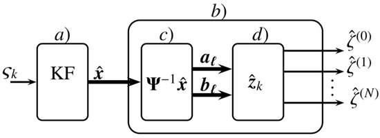
Figure 1. Block diagram describing the proposed methodology to estimate the FCs, DFCs, signal approximation and its derivatives. In (a), the Kalman filter is implemented, (b) contains two subsections, (c) and (d). In (c) the coefficients with the state estimates provided by Kalman filter and with the state matrix ${\mathsf{\Psi }}^{-1}$ are obtained. Finally in block (d) Equation (18a)–(18d) is implemented to obtain the approximation signal.

The output of the Kalman algorithm is the input of a second stage, as seen in Figure 1 (b), which is divided into two subsections, Figure 1 (c) and (d). The coefficients are obtained by the block in Figure 1 (c) with the state matrix ${\mathsf{\Psi }}^{-1}$ and $\widehat{x}$ (as is illustrated in (17). Finally, with the coefficient estimates $a_{\ell }$ and $b_{\ell }$ implemented in Equation (18a)–(18c) by the block of Figure 1 (d), the approximations to the signal ${\widehat{\zeta }}^{\left(0\right)}$ and its derivatives ${\widehat{\zeta }}^{\left(1\right)},{\widehat{\zeta }}^{\left(2\right)},\dots ,{\widehat{\zeta }}^{\left(M\right)},$ are obtained and are the output of the block diagram. Note that the last block in Figure 1 represents the procedure code that is shown in Algorithm 2, and thus the process is completed.

4. Performance of the Harmonic Filters

In this section, the performance of the proposed algorithm is shown. When the signal model is approximated with $M=0$ in the polynomial form, defined in (2), the signal model is equivalent to the model proposed in [20] and here is named a Kalman filter algorithm (KFA). When the order signal approximation in the model is $M>0$ and $\ell >1$, the proposed algorithm is named a Taylor–Kalman–Fourier algorithm (TKFA). On the other hand, the filters are tested with a square wave signal as an input and are compared with DFT, and KFA. The results are illustrated in Figure 2, where the behavior between DFT, KFA and TKFA are very similar. Additionally, the zoom shows in detail the behavior of the estimates, and it can be seen that the precision of the methods is equivalent. To obtain more precise results in the comparison of the algorithms, the RMS Error defined by

$$RMSE=\sqrt{{\left(\frac{{\sum }_{n=1}^{N}s\left[n\right]-\widehat{\zeta }\left[n\right]}{N}\right)}^2},$$

(19)

is obtained with respect to the measurement input signal $s\left[n\right]$ and its estimate $\zeta \left[n\right]$. The obtained results are shown in Table 1 for a different number of harmonics in the signal model by KFA and TKFA. The number of harmonics implemented in the model is represented by $\omega$. Hence, ${\omega }_f$ represents the fundamental model, and therefore, the transition matrix $\mathsf{\Psi }$ is developed only with $\ell =1$. Note that the results obtained by the three algorithms are equivalent. However, with the DFT and KFA, the DFCs cannot be obtained. Thus, the results of the RMS error in Table 1 are obtained only using the coefficients a and b.

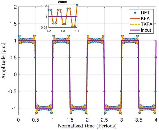
Figure 2. Reconstruction signal with DFT, KFA, and TKFA algorithms. The model considers 15 harmonic components.

Table 1. RMS Error (RMSE) obtained with DFT, KFA and TKFA with respect to the input signal and the approximation to the measurement signal ${\widehat{\zeta }}^{\left(0\right)}$.

RMSE
	$\mathbf{\omega }$	DFT	KFA	TKFA	$\mathbf{\omega }$	DFT	KFA	TKFA
Square signal	${\omega }_f$	$0.430$	$0.430$	$0.430$	${\omega }_8$	$0.187$	$0.187$	$0.187$
	${\omega }_1$	$0.430$	$0.430$	$0.430$	${\omega }_9$	$0.187$	$0.187$	$0.187$
	${\omega }_2$	$0.308$	$0.308$	$0.308$	${\omega }_{10}$	$0.167$	$0.167$	$0.167$
	${\omega }_3$	$0.308$	$0.308$	$0.308$	${\omega }_{11}$	$0.167$	$0.167$	$0.167$
	${\omega }_4$	$0.249$	$0.249$	$0.249$	${\omega }_{12}$	$0.151$	$0.151$	$0.151$
	${\omega }_5$	$0.249$	$0.249$	$0.249$	${\omega }_{13}$	$0.151$	$0.151$	$0.151$
	${\omega }_6$	$0.213$	$0.213$	$0.213$	${\omega }_{14}$	$0.137$	$0.137$	$0.137$
	${\omega }_7$	$0.213$	$0.213$	$0.213$	${\omega }_{15}$	$0.137$	$0.137$	$0.137$
Sawtooth Signal	${\omega }_f$	$0.069$	$0.069$	$0.069$	${\omega }_8$	$85\times {10}^{-4}$	$85\times {10}^{-4}$	$85\times {10}^{-4}$
	${\omega }_1$	$0.069$	$0.069$	$0.069$	${\omega }_9$	$85\times {10}^{-4}$	$85\times {10}^{-4}$	$85\times {10}^{-4}$
	${\omega }_2$	$0.028$	$0.028$	$0.028$	${\omega }_{10}$	$68\times {10}^{-4}$	$68\times {10}^{-4}$	$68\times {10}^{-4}$
	${\omega }_3$	$0.028$	$0.028$	$0.028$	${\omega }_{11}$	$68\times {10}^{-4}$	$68\times {10}^{-4}$	$68\times {10}^{-4}$
	${\omega }_4$	$0.016$	$0.016$	$0.016$	${\omega }_{12}$	$57\times {10}^{-4}$	$57\times {10}^{-4}$	$57\times {10}^{-4}$
	${\omega }_5$	$0.016$	$0.016$	$0.016$	${\omega }_{13}$	$57\times {10}^{-4}$	$57\times {10}^{-4}$	$57\times {10}^{-4}$
	${\omega }_6$	$0.011$	$0.011$	$0.011$	${\omega }_{14}$	$49\times {10}^{-4}$	$49\times {10}^{-4}$	$49\times {10}^{-4}$
	${\omega }_7$	$0.011$	$0.011$	$0.011$	${\omega }_{15}$	$49\times {10}^{-4}$	$49\times {10}^{-4}$	$49\times {10}^{-4}$

A second signal is tested and is illustrated in Figure 3. Additionally, its approximation is obtained with DFT, KFA, and TKFA. The zoom shows in detail the behavior of the estimates, and it can be seen that the precision of the methods is equivalent between DFT and KFA, but TKFA has a litter discrepancy in the estimation provided by the signal model, where the harmonics are included.

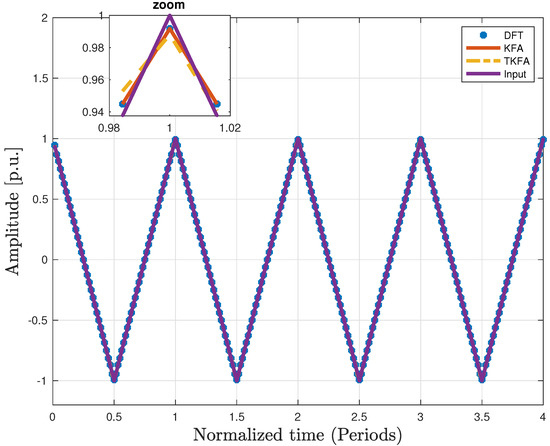
Figure 3. Reconstruction signal with DFT, KFA and TKFA algorithms. In this case, the model of KFA and TKFA was constructed with the full set of harmonics components (64 harmonics).

We propose to select this signal because its derivative is intuitive and easy to obtain. On the other hand, with the coefficients $a_1$ and $b_1$ obtained with (17) and implemented in (18b), we achieved approximation to the derivative of the signal, and the results are presented in Figure 4 where the path trajectory is the expected result because the derivative of a sawtooth signal is a square signal. The zoom shows in detail the behavior of the estimates. As the coefficients $a_1$ and $b_1$ are not possible to obtain with DFT and KFA, the approximation to the derivative ${\widehat{\zeta }}^{\left(1\right)}$ in Figure 4 only represents the estimates with TKFA.

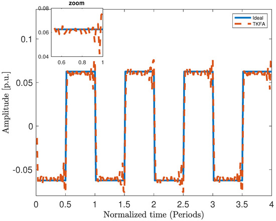
Figure 4. Derivative approximation to the input signal with TKFA algorithm.

With the proposal to make an analysis of the noise effect, Figure 5 shows the frequency responses of DFT, KFA and TKFA. The zoom shows in detail the behavior of the estimates. Using KFA and TKFA, the frequency response can be obtained using

$$G\left(z\right)={\left[I+\left(KH-I\right)\mathsf{\Psi }{z}^{-1}\right]}^{-1}K.$$

(20)

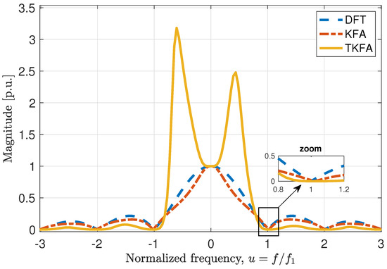
Figure 5. Magnitude response of DFT, KFA and TKFA algorithms, with $Q={10}^{-3}$, $P_r={10}^{10}$ and $R=1$.

The results illustrated in Figure 5 were developed using the next parameters in the KFA and TKFA, $Q={10}^{-3}$, $R=1$ and $P_r={10}^{10}$.

In Figure 6 the frequency response is illustrated with $Q={10}^{-1}$, $P_r={10}^{10}$ and $R=1$. The zoom shows in detail the behavior of the estimates.

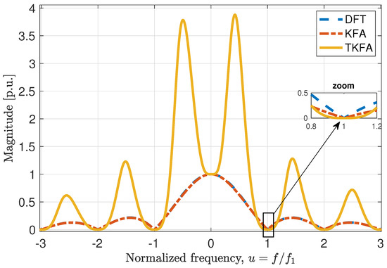
Figure 6. Magnitude response of DFT, KFA and TKFA algorithms with $Q={10}^{-1}$, $P_r={10}^{10}$ and $R=1$.

The comparison between Figure 5 and Figure 6 show how the inter-harmonic amplitude decreases in KFA and TKFA when the value in Q decreases. However, the decrement in the inter-harmonic amplitude is more significant in TKFA. A similar study of the noise was made in [20], where a complementary study was made of the spectral and short-time analysis. As TKFA achieves a null-flat frequency response around the frequency operation and its harmonics, the proposed method can achieve better results in applications where frequency and harmonics have a few distortions. For example, when the rotor bar has litter damage, the current has a frequency shift [24].

5. Conclusions

The aim of this work is the development of a method to estimate the coefficients of an input signal and the coefficients of the derivative input signal. To achieve the coefficient estimates, we develop a method that consists of two stages. First, a proposed signal model is implemented in the Kalman filter, and with this model, we are able to estimate the derivatives of the input signal. Second, with the state prediction and the inverse of the state matrix, the coefficients of the signal and the coefficients of the successive derivatives are obtained. On the other hand, in comparison to the DFT, the new class of filters provides advantages in the sense of noise reduction and the sidelobe suppression. Additionally, the proposed TKFA achieves a null-flat frequency response around the frequency operation. Moreover, with the proposed TKFA method, the decrement in the inter-harmonic amplitude is greater than that obtained with KFA, and the neighborhood of the null-flat frequency is expanded. The approximation to the input signal and its derivative can be achieved with a sum of functions that are related by the estimate coefficients and their respective harmonics. Thereby, the proposed method is related to the Fourier series. However, with the new filters, it is possible to estimate the derivative Fourier series with the derivative coefficient estimates.

References

- Saima, S.; Li, B.; Adnan, S.M. New Sampling Expansion Related to Derivatives in Quaternion Fourier Transform Domain. Mathematics 2022, 10, 1217. [Google Scholar] [CrossRef]
- Ruibo, J.; Xiaoqiang, L. Using Fourier series to fit The GPS precise ephemeris. In Proceedings of the 2010 International Conference on Computer Application and System Modeling (ICCASM 2010), Taiyuan, China, 22–24 October 2010; Volume 11, pp. V11-96–V11-99. [Google Scholar] [CrossRef]
- Labiod, S.; Boubertakh, H.; Guerra, T.M. Fourier series-based adaptive tracking control for robot manipulators. In Proceedings of the 3rd International Conference on Systems and Control, Algiers, Algeria, 29–31 October 2013; pp. 968–972. [Google Scholar] [CrossRef]
- Gholipour, R.; Fateh, M.M. Adaptive task-space control of robot manipulators using the Fourier series expansion without task-space velocity measurements. Measurement 2018, 123, 285–292. [Google Scholar] [CrossRef]
- Van den Bos, A. Best linear unbiased estimation of the Fourier coefficients of periodic signals. IEEE Trans. Instrum. Meas. 1993, 42, 49–51. [Google Scholar] [CrossRef][Green Version]
- Harris, F.J. On the use of windows for harmonic analysis with the discrete Fourier transform. Proc. IEEE 1978, 66, 51–83. [Google Scholar] [CrossRef]
- Hostetter, G. Recursive discrete Fourier transformation. IEEE Trans. Acoust. Speech Signal Process 1980, 28, 184–190. [Google Scholar] [CrossRef]
- Varkonyi-Koczy, A.R. A recursive fast Fourier transformation algorithm. IEEE Trans. Circuits Syst. II Analog Digit. Signal Process 1995, 42, 614–616. [Google Scholar] [CrossRef]
- Fan, C.P.; Su, G.A. Novel recursive discrete Fourier transform with compact architecture. In Proceedings of the 2004 IEEE Asia-Pacific Conference on Circuits and Systems, Tainan, Taiwan, 6–9 December 2004; Volume 2, pp. 1081–1084. [Google Scholar] [CrossRef]
- Park, S.H.; Kim, M.J.; Kwon, W.H.; Kwon, O.K. Short-time harmonic analysis via the state-space optimal FIR filter. In Proceedings of the SICE ’95, 34th SICE Annual Conference, Hokkaido, Japan, 26–28 July 1995; International Session Papers. pp. 1205–1210. [Google Scholar] [CrossRef]
- Park, S.H.; Kwon, W.H.; Kwon, O.K.; Kim, M.J. Short-time Fourier analysis via optimal harmonic FIR filters. IEEE Trans. Signal Process 1997, 45, 1535–1542. [Google Scholar] [CrossRef]
- Li, W. Alternative Fourier Series Expansions with Accelerated Convergence. Appl. Math. 2016, 7, 1824–1845. [Google Scholar] [CrossRef]
- Xiao, Y.; Tadokoro, Y.; Shida, K. Adaptive algorithm based on least mean p-power error criterion for Fourier analysis in additive noise. IEEE Trans. Signal Process 1999, 47, 1172–1181. [Google Scholar] [CrossRef]
- Nishi, K. Kalman filter analysis for quasi-periodic signals. In Proceedings of the 2001 IEEE International Conference on Acoustics, Speech, and Signal Processing, Proceedings (Cat. No.01CH37221), Salt Lake City, UT, USA, 7–11 May 2001; Volume 6, pp. 3937–3940. [Google Scholar] [CrossRef]
- Gruber, P.; Todtli, J. Estimation of quasiperiodic signal parameters by means of dynamic signal models. IEEE Trans. Signal Process 1994, 42, 552–562. [Google Scholar] [CrossRef]
- Kim, T.; Kim, D.; Jang, L.C.; Jang, G.W. Fourier Series for Functions Related to Chebyshev Polynomials of the First Kind and Lucas Polynomials. Mathematics 2018, 6, 276. [Google Scholar] [CrossRef]
- Sefusatti, E.; Crocce, M.; Scoccimarro, R.; Couchman, H.M.P. Accurate estimators of correlation functions in Fourier space. Mon. Not. R. Astron. Soc. 2016, 460, 3624–3636. [Google Scholar] [CrossRef]
- Gilbert, A.C.; Guha, S.; Indyk, P.; Muthukrishnan, S.; Strauss, M. Near-Optimal Sparse Fourier Representations via Sampling. In Proceedings of the Annual ACM Symposium on Theory of Computing, Montreal, QC, Canada, 19–21 May 2002; pp. 152–161. [Google Scholar] [CrossRef]
- Yu, W.; Yong, Y.; Guan, G.; Huang, Y.; Su, W.; Cui, C. Valuing Guaranteed Minimum Death Benefits by Cosine Series Expansion. Mathematics 2019, 7, 835. [Google Scholar] [CrossRef]
- Bitmead, R.; Tsoi, A.; Parker, P. A Kalman filtering approach to short-time Fourier analysis. IEEE Trans. Acoust. Speech Signal Process 1986, 34, 1493–1501. [Google Scholar] [CrossRef]
- Zhang, B.; Pong, M.H. Dynamic model and small signal analysis based on the extended describing function and Fourier series of a novel AM ZVS direct coupling DC/DC converter. In Proceedings of the Power Processing and Electronic Specialists Conference, Atlantic City, NJ, USA, 22–23 May 1997; Volume 1, pp. 447–452. [Google Scholar] [CrossRef]
- Manolakis, D.G.; Ingle, V.K.; Kogon, S.M. Statistical and Adaptive Signal Processing: Spectral Estimation, Signal Modeling, Adaptive Filtering and Array Processing; Artech House Publishers: Boston, MA, USA, 2005. [Google Scholar]
- Simon, D. Optimal State Estimation: Kalman, H Infinity, and Nonlinear Approaches; John Wiley & Sons: Hoboken, NJ, USA, 2006. [Google Scholar]
- Trujillo-Guajardo, L.A.; Rodriguez-Maldonado, J.; Moonem, M.A.; Platas-Garza, M.A. A Multiresolution Taylor–Kalman Approach for Broken Rotor Bar Detection in Cage Induction Motors. IEEE Trans. Instrum. Meas. 2018, 67, 1317–1328. [Google Scholar] [CrossRef]
Publisher’s Note: MDPI stays neutral with regard to jurisdictional claims in published maps and institutional affiliations. |
© 2022 by the authors. Licensee MDPI, Basel, Switzerland. This article is an open access article distributed under the terms and conditions of the Creative Commons Attribution (CC BY) license (https://creativecommons.org/licenses/by/4.0/).