Learning EOQ Model with Trade-Credit Financing Policy for Imperfect Quality Items under Cloudy Fuzzy Environment

Abstract

An imprecise demand rate creates problems in profit optimization in business scenarios. The aim is to nullify the imprecise nature of the demand rate with the help of the cloudy fuzzy method. Traditionally, all items in an ordered lot are presumed to be of good quality. However, the delivered lot may contain some defective items, which may occur during production or maintenance. Inspection of an ordered lot is indispensable in most organizations and can be treated as a type of learning. The learning demonstration, a statistical development expressing declining cost, is necessary to achieve any cyclical process. Further, defective items are sold immediately after the screening process as a single lot at a discounted price, and the fraction of defective items follows an S-shaped learning curve. The trade-credit policy is adequate for suppliers and retailers to maximize their profit during business. In this paper, an inventory model is developed with learning and trade-credit policy under the cloudy fuzzy environment where the demand rate is treated as a cloudy fuzzy number. Finally, the retailer’s total profit is maximized with respect to order quantity. Sensitivity analysis is presented to estimate the robustness of the model.

1. Basic Introduction

The present paper describes techniques and recent developments in inventory management. It covers a summary of literature reviews, research gaps, and the development of the paper.

1.1. Introduction

In the economic order quantity (EOQ) model, all produced items are considered to be of good quality in nature. Defects may arise due to practically instant power outages or delays in the supply of raw materials, leading to the production of defective items. Because it is impossible to produce 100% good-quality items during manufacturing, many companies appoint an inspector to inspect the quality of items by separating defective and none defective items. Therefore, the inspection process is unavoidable. In this paper, inspected items are classified into two categories, viz., non defective items and defective items. During the inspection process, the screening rate must be more than the demand rate to avoid shortages and satisfy consumer demand for perfect items parallel to the screening process. Further, defective items are sold immediately after the screening process as a single lot at a discounted price. This paper investigates the impact of learning on retailer ordering policy for imperfect-quality items with trade-credit financing under in-process inspection, where the demand rate is taken as a cloudy fuzzy number. The numerical example reveals that the proposed model with the defuzzification method maximizes retailer profit. Finally, sensitivity analysis is performed to show the novelty of the proposed model. The contribution of the authors is defined in the Table 1.

Table 1. Contribution of different authors.

Author(s)	Learning Effects	Inspection	Trade-Credit Financing	Imperfect Items	Cloudy Fuzzy Environment
Wright [10]
Hammer [23]
Baloff [24]
Cunningham [25]
Dutton [26]
Argote et al. [27]
Salameh et al. [28]
Jaber and Bonney [11]
Aggrawal and Jaggi [8]
Salameh and Jaber [29]
Jaber et al. [30]
Khan et al. [31]
Anazanello and Fogliatto [32]
Jaggi et al. [13]
Jaggi et al. [19]
Sarkar [33]
Sangal et al. [34]
Shin et al. [35]
Jaggi et al. [36]
Jayaswal et al. [15]
Patro et al. [21]
Nobil et al. [37,38]
De and Mahata [22]
Present paper

1.2. Literature Review

A mathematical model was developed by [1] at the beginning of the 19th century. Many authors have proposed mathematical models with imperfect-quality items in the field of inventory management. Primary models have been extended with new approaches in an attempt to improve on the flaws of existing models. Ref. [2], suggested a mathematical model for the nature and structure of inventory problems.

Ref. [3], developed a mathematical model that included the impact of defective items with the help of the EOQ basic model and assumed that a lot has a percentage of defective items that follow a geometric distribution. [4], discussed the time between the start of production until the control situation in the presence of defective items. Subsequently, [5] presented a mathematical model using the concept of inspection and corrected the control situation of the production process. The most popular mathematical models were developed by [6,7]. Ref. [8], proposed a method for decaying items in the field of inventory management where deteriorating items were kept constant. Ref. [9], proposed an EOQ model for deteriorating items where the demand rate was kept constant for the EOQ model. The behavior of the learning curve was presented by [10]. Ref. [11], presented an EOQ model for lot-sizing problems under learning considerations. Ref. [12], derived a mathematical model for lot-sizing problems under learning and forgetting. Ref. [13], proposed an inventory model with permissible delay in payment under shortages for imperfect items. Ref. [14], considered a sustainable inventory management method with deteriorating and imperfect-quality items considering carbon emissions. Ref. [15], explained a learning concept for imperfect items with a permissible delay in payment and optimized order quantity and retailer profit in a mathematical model. Ref. [16], proposed an inventory model for supply model with imperfect quality items where demand rate is a function of price and marketing expenditure. Ref. [17], presented an inventory model for new product launching with pricing, free replacement, rework, and warranty policies via genetic algorithmic approach.

Refs. [15,18], explained the EOQ mathematical representation of stock for decaying items with the influence of inspection in fuzzy systems under the credit financing strategy and shortages. Ref. [18], discussed an EOQ model for decaying items under a fuzzy environment with time-dependent demand and shortages. Ref. [19], developed an economic order quantity using a fuzzy environment under the credit financing policy and shortages. Ref. [20], proposed the finest refill strategy for cost-reliant orders in different economic situations under the fuzzy concept. Ref. [21], introduced a fuzzy environment for decaying items under the effect of learning with defective feature items with the help of fair concessions. The commendable work of [22] is improved by this paper with the help of the learning effect and credit financing where defective items follow an S-shaped learning curve. Conclusively, sensitivity analysis is presented as a result of numerical examples.

1.3. Research Gap

Following a literature review, this section covers the models and effects of the EOQ model: EOQ model for defective items, EOQ model for defective items under learning effects, EOQ model with trade credit under learning effects, and EOQ model for defective items under the cloudy fuzzy number. Additionally, it is observed from the table of contributions that no research paper has been published since 1936 on learning and trade-credit financing for defective items under the cloudy fuzzy environment. This motivated the authors of this paper to develop a mathematical inventory model with learning and trade-credit financing policy for defective items under the cloudy fuzzy environment. The present work, summarized in the bottom row of the Table 1 of contributions with specific keywords, attempts to bridge the research gap from 1936 to 2021 with learning and trade-credit financing under the cloudy fuzzy environment. A frame diagram of the proposed model is shown in Figure 1.

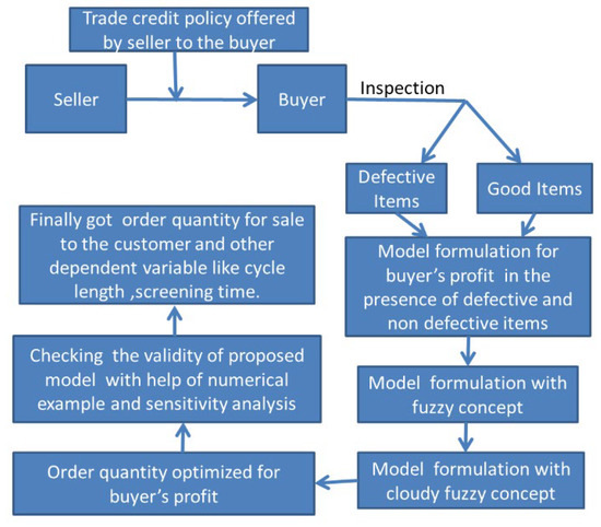
Figure 1. Frame diagram for the proposed model.

2. Preliminary Definition

Some definitions required for the proposed model are given below [22].

Definition 1.

When we consider the model for a fuzzy environment, the following definitions are necessary. A fuzzy set$\tilde{A}$on the universal set is$X$denoted and defined by

$$\tilde{A}=\left\{\left(x,\hspace{0.17em}{\lambda }_{\tilde{A}}\left(\tilde{x}\right)\right):\hspace{0.17em}x\in X\right\}$$

where${\lambda }_{\tilde{A}}:X\to \left[0,\hspace{0.17em}1\right]$is known as the membership function.

The triplet$\left(x_1,x_2,x_3\right)$is used to specify a triangular fuzzy number$\left(x_1,x_2,x_3\right)$and is defined by the continuous membership function$\tilde{\lambda }:X\to \left[0,1\right]$such that

$${\lambda }_{\tilde{A}}=\left\{\begin{array}{l}\frac{x-x_1}{x_2-x_1},x_1\le x\le x_2\\ \frac{x_3-x_1}{x_3-x_2},x_2\le x\le x_3\\ 0,\hspace{0.17em}\hspace{0.17em}\hspace{0.17em}\hspace{0.17em}\mathrm{Otherwise}\end{array}\right.$$

Definition 2.

For any $c$and $0\in R$, the signed distance from$c$to$0$is$d\left(c,0\right)=c$, and if$c<0$, the signed distance from$c$is$d\left(-c,0\right)=-c$. Suppose$\Omega$is the family of all fuzzy sets$\tilde{B}$defined on$R$for which the$\alpha -$cut$B\left(\alpha \right)=\left[B_L\left(\alpha \right),B_L\left(\alpha \right)\right]$exists for every$\alpha \in \left[0,1\right]$, and both$B_L\left(\alpha \right)$and$B_U\left(\alpha \right)$are continuous functions on$\alpha \in \left[0,1\right]$. Then, for$\tilde{B}\in \Omega$, we have$B\left(\alpha \right)=\underset{0\le \alpha \le 1}{U}\left[B_L{\left(\alpha \right)}_{\alpha },B_L{\left(\alpha \right)}_{\alpha }\right].$

Definition 3.

For$\tilde{C}\in \Omega$, define the signed distance from$\tilde{B}$to${\tilde{0}}_1$as

$$d\left(\tilde{B},\tilde{0}\right)=\frac{1}{2}{\displaystyle {\int }_0^1\left({\tilde{B}}_L\left(\alpha \right)+{\tilde{B}}_R\left(\alpha \right)\right)}\hspace{0.17em}d\alpha$$

(1)

Definition 4.

If$\tilde{A}=\left(x_{1,}{x}_2,x_3\right)$is a triangular fuzzy number, then the$\alpha -$cut of$\tilde{A}$is$A\left(\alpha \right)=\left[A_L\left(\alpha \right),A_U\left(\alpha \right)\right]$for$\alpha \in \left[0,1\right]$, where$A_L\left(\alpha \right)=x_1+\left(x_2-x_1\right)\alpha$, and$A_U\left(\alpha \right)=x_3-\left(x_3-x_2\right)\alpha$. Then, the signed distance from$\tilde{A}$to${\tilde{0}}_1$is

$$d\left(\tilde{A},\hspace{0.17em}\tilde{0}\right)=\frac{\left(x_1+2x_2+x_3\right)}{4}$$

(2)

Definition 5.

Yager’s Ranking Index.

Let$B_L\left(\alpha \right)$and$B_U\left(\alpha \right)$be the left and right$\alpha -$cuts of a fuzzy number$\tilde{a}$. The defuzzification rule under Yager’s ranking index as suggested by [22] is given as

$$I\left(\tilde{a}\right)=\frac{1}{2}{{\displaystyle \int }}_0^1\left(B_L\left(\alpha \right)+B_R\left(\alpha \right)\right)d\alpha$$

(3)

Definition 6.

Cloudy Normalized Triangular Fuzzy Number.

A fuzzy number of the form$\tilde{L}=\left(l_{1, }{l}_{2,}{l}_{3, }\right)$is called a triangular fuzzy number if, after an infinite time, the set itself converges to a crisp singleton. Mathematically, it can be represented by$t\to \infty$. Then, $l_{1, }{l}_{3, }\tilde{L}\to \left\{l_2\right\},$and it can be considered that the fuzzy numbers are$\tilde{L}=\left(l_2\left(1-\frac{\rho }{1+t}\right), l_2, l_2\left(1+\frac{\sigma }{1+t}\right)\right)$for$0<\rho ,\sigma <1$. Here, note that$\underset{}{\underset{t\to \infty }{\lim }\hspace{0.17em}\hspace{0.17em}{l}_2\left(1-\frac{\rho }{1+t}\right)=l_2}$and$\underset{}{\underset{t\to \infty }{\lim }\hspace{0.17em}\hspace{0.17em}{l}_2\left(1-\frac{\sigma }{1+t}\right)=l_2}$.

Now, it can be easily seen that$\tilde{L}\to \left\{l_2\right\}$.

The membership function [6] that can be defined for$0\le t$is as follows:

$$f\left(x,t\right)=\left\{\begin{array}{l}0\hspace{0.17em}\hspace{0.17em}\hspace{0.17em}\hspace{0.17em}\hspace{0.17em}\hspace{0.17em}\hspace{0.17em}\hspace{0.17em}\hspace{0.17em}\hspace{0.17em}\mathrm{if}\hspace{0.17em}\hspace{0.17em}x⟨l_2\left(1-\frac{\rho }{1+t}\right)\hspace{0.17em}\hspace{0.17em}\mathrm{and}\hspace{0.17em}\hspace{0.17em}\hspace{0.17em}x⟩\hspace{0.17em}{l}_2\left(1+\frac{\sigma }{1+t}\right)\\ \frac{x-l_2\left(1-\frac{\rho }{1+t}\right)}{\frac{\rho l_2}{1+t}}\hspace{0.17em}\mathrm{if}\hspace{0.17em}\hspace{0.17em}\hspace{0.17em}\hspace{0.17em}\hspace{0.17em}{l}_2\left(1-\frac{\rho }{1+t}\right)\le x\le l_2\\ \frac{l_2\left(1+\frac{\sigma }{1+t}\right)-x}{\frac{\sigma l_2}{1+t}}\hspace{0.17em}\mathrm{if}\hspace{0.17em}\hspace{0.17em}\hspace{0.17em}\hspace{0.17em}\hspace{0.17em}\hspace{0.17em}{l}_2\le x\le l_2\left(1+\frac{\sigma }{1+t}\right)\end{array}\right.$$

(4)

Definition 7.

Ranking Index over Cloudy Normalized Triangular Fuzzy Number (CNTFN).

Let us take the left and right$\alpha -\mathrm{cuts}$off (x, t) from (5), noted as$A\left(\alpha ,t\right)$and$B\left(\alpha ,t\right)$, respectively. Then, the defuzzification formula under the time extension of Yeager’s ranking index is given by

$$I\left(\tilde{L}\right)=\frac{1}{2T}{\displaystyle {\int }_{\alpha =0}^{\alpha =1}{\displaystyle {\int }_{t=0}^{t+T}\left\{A^{-1}\left(\alpha ,t\right)+B^{-1}\left(\alpha ,t\right)\right\}d\alpha \hspace{0.17em}dT}}$$

(5)

where$\alpha$and$t$are independent variables. Let us suppose that$\tilde{L}$is a CNTFN state in Equation (4) with its membership function in Equation (5). Now, utilizing Equation (5), the left and right$\alpha -\mathrm{cuts}$off (x, t) are given by

$$A^{-1}\left(\alpha ,t\right)=l_2\left(1-\frac{\rho }{1+t}+\frac{\rho \sigma }{1+t}\right)$$

(6)

and

$$B^{-1}\left(\alpha ,t\right)=l_2\left(1+\frac{\sigma }{1+t}+\frac{\rho \sigma }{1+t}\right)$$

(7)

Thus, Equation (5) will become

$$I\left(\tilde{L}\right)=\frac{l_2}{2T}\left[2T+\frac{\sigma -\rho }{2}\log \left(1+T\right)\right]$$

(8)

Equation (8) can be written as$I\left({\displaystyle \tilde{L}}\right)=\hspace{0.17em}\frac{l_2}{2T}\left[1+\frac{\sigma -\rho }{4}\frac{\log \left|1+T\right|}{T}\right]$. It can be easily seen that$\underset{T\to \infty }{\lim }\frac{\log \left(1+T\right)}{T}=0$; therefore, $I\left(\tilde{L}\right)\to l_2$as$T\to \infty$, the factor$\frac{\log \left(1+T\right)}{T}$is known as the cloud index (CT), and the time is measured by days in practice. The behavior of cloud indexes with time in days is shown below in Figure 2.

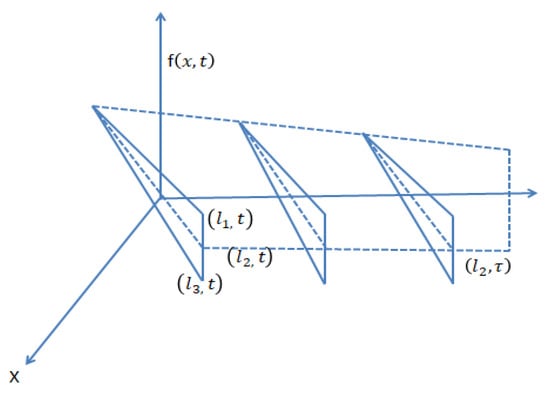
Figure 2. Representation of triangular fuzzy number.

3. Assumptions

Following assumptions are used in the model.

⮚

The replenishment is assumed to be immediate.

⮚

Shortages are not allowed, and the lead time is negligible.

⮚

A trade-credit financing strategy is allowed by the supplier to the retailer [13].

⮚

It is considered that the rate of demand is less than the inspection rate [13].

⮚

The time horizon is finite.

⮚

The demand rate is considered as a cloudy fuzzy triangular number.

⮚

It is assumed that the ordered lot has some defective items [29].

⮚

Defective percentages present in each lot follow the behavior of the learning curve, as suggested by [30].

⮚

Defective items are sold at a rebate discount after the inspection process.

4. Formulation of Crisp Mathematical Model

A numerical model is created under permissible delay in payments considering the impact of learning on defective items. It is assumed that a batch of $Q$ units goes into the inventory system at $t=0,$ and the ordered batch contains s $p\left(n\right)$ defective items (Figure 3). The entire lot goes through an inspection process at a constant $\lambda$ unit/time rate and separates defective and defective items after the inspection process. Further, a presumption is made to inspect the defective items at a predefined rate of $\left(1-p\left(n\right)\right)\chi$ in the time period $t_n=\frac{Q}{\chi }$, and good-quality items fulfil the demand with rate $D.$ After the inspection process at $t_n$, the imperfect items are traded as a defective batch at a low price $c_s$. It is assumed that imperfect items $p\left(n\right)$ satisfy the given condition $\left(1-p\left(n\right)\right)\chi \ge D{t}_n$, which infers that $p\left(n\right)\le 1-\frac{D}{\chi }$, where $t_n=\frac{Q}{\chi }$ to avoid shortages. The supplier offers the retailer a predetermined credit period, say, $M$, to inspire sales. As a result, depending on the credit period, there are three distinct conditions for the retailer: (i) $T_n\ge t_n\ge M$, (ii) $T_n\ge M\ge t$, and (iii) $M\ge T_n\ge t_n$.

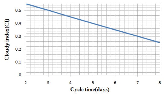
Figure 3. Behavior of fuzziness over time.

The cycle length $T_n$ for the planned inventory form is specified by

$$T_n=\frac{\left(1-p\left(n\right)\right)Q}{D}$$

(9)

Time to screen $Q$ units ordered per cycle is specified by

$$t_n=\frac{Q}{\chi }$$

(10)

The retailer’s total profit $\Psi \left(Q\right)$ contains the subsequent components, which are given below (see Figure 4).

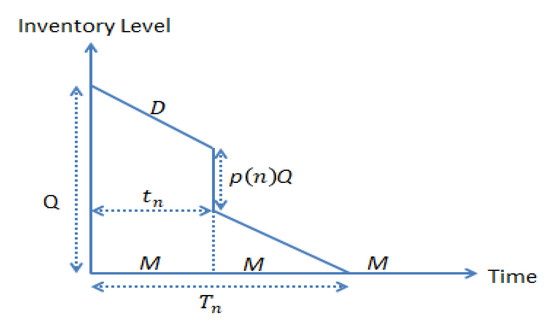
Figure 4. Inventory system with trade-credit financing.

$\Psi \left(Q\right)$ = total revenue − set up cost − purchasing price − inspection cost − carrying cost + interest gained − interest charged.

$$\Psi \left(Q\right)=s(1-p(n))Q+vp(n)Q-k-cQ-dQ-h\left(\frac{T_n\left(1-p(n)\right)Q}{2}+\frac{Q^{2}p\left(n\right)}{\chi }\right)+IE-IP$$

The retailer’s whole profit per cycle is

$$\Psi \left(Q\right)=\frac{s(1-p(n))Q+vp(n)Q-k-cQ-dQ-h·\left(\frac{T_n\left(1-p(n)\right)Q}{2}+\frac{Q^{2}p\left(n\right)}{\chi }\right)+IE-IP}{T_n}$$

(11)

The calculation of interest earned $\left(IE\right)$ and charged $\left(IP\right)$ can be calculated case wise and is mentioned below.

Case 1: $0\le M\le t_n\le T_n$

In this case, the retailer earns profit on total income from the credit period up to M, which is equal to $I_{e}pD{M}^2/2$, and the interest to be paid for unsold items from the period $M$ to $T_n$ is equal to $c{I}_p{T}_n\hspace{0.17em}D\hspace{0.17em}{\left(T_n-M\right)}^2/2+c_{}{I}_{p}p\left(n\right)y_n\left(t_n-M\right)$, shown in Figure 5.

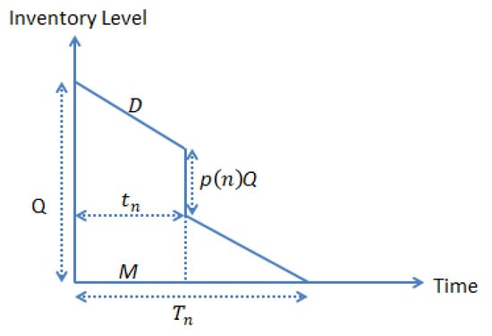
Figure 5. Inventory system for Case 1.

The retailer’s total profit is given as

$${\Psi }_1\left(Q\right)=\frac{\begin{array}{l}s(1-p(n))Q+vp(n)Q-k-cQ-dQ-h\left(\frac{T_n\left(1-p(n)\right)Q}{2}+\frac{Q^{2}p\left(n\right)}{\chi }\right)\\ +I_{e}pD{M}^2/2-c{I}_p{T}_n\hspace{0.17em}D\hspace{0.17em}\hspace{0.17em}{\left(T_n-M\right)}^2/2+c{I}_{p}p\left(n\right)Q\left(t_n-M\right)\end{array}}{T_n}$$

The retailer’s total profit per cycle is given as

$$\begin{array}{l}{\Psi }_1\left(Q\right)=sD+\frac{vDp(n)}{1-p(n)}+\frac{D^2{M}^2(I_{e}p-I_{p}c)}{2(1-p(n))Q}-\frac{KD}{(1-p(n))Q}\\ -\frac{(c+d-c_s{I}_{p}p(n)M-c.I_p(1-p(n)M)D}{1-p(n)}-\\ \frac{\left[h\left(\frac{{(1-p(n))}^2}{2D}+\frac{p(n)}{\chi }\right)+\frac{c{I}_p{(1-p(n))}^2}{2D}+\frac{c_s{I}_{p}p(n)}{\chi }\right]QD}{1-p(n)}\end{array}$$

(12)

To maximize the total profit per cycle for the given value of $Q$ taking the first derivative of Equation (12), we get

$$\frac{{\Psi }_1\left(Q\right)}{dQ}=-\frac{D^2{M}^2(I_{e}p-I_{p}c)}{2(1-p(n))Q^2}+\frac{KD}{(1-p(n))Q^2}\hspace{0.17em}-\frac{\left[\begin{array}{l}h\left(\frac{{(1-p(n))}^2}{2D}+\frac{p(n)}{\chi }\right)\\ +\frac{c{I}_p{(1-p(n))}^2}{2D}+\frac{c_s{I}_{p}p(n)}{\chi }\end{array}\right]D}{1-p(n)}$$

$$If\frac{d\hspace{0.17em}{\Psi }_1\left(Q\right)}{dQ}=0=-\frac{D^2{M}^2(I_{e}p-I_{p}c)}{2(1-p(n))Q^2}+\frac{KD}{(1-p(n))Q^2}\hspace{0.17em}-\frac{\left[\begin{array}{l}h\left(\frac{{(1-p(n))}^2}{2D}+\frac{p(n)}{\chi }\right)\\ +\frac{c{I}_p{(1-p(n))}^2}{2D}+\frac{c_s{I}_{p}p(n)}{\chi }\end{array}\right]D}{1-p(n)}=0$$

(13)

After solving Equation (13) for $Q$, the value of $Q$ is equal to

$$Q=\sqrt{\frac{\frac{D^2{M}^2(I_{e}p-I_{p}c)}{2(1-p(n))}-\frac{KD}{(1-p(n))}}{\frac{\left[h\left(\frac{{(1-p(n))}^2}{2D}+\frac{p(n)}{\chi }\right)+\frac{c{I}_p{(1-p(n))}^2}{2D}+\frac{c_s{I}_{p}p(n)}{\chi }\right]D}{1-p(n)}}}$$

(14)

Taking the second derivative of Equation (12) with respect to $Q$ will be equal to

$$\frac{d^2\hspace{0.17em}{\Psi }_1\left(Q\right)}{d{Q}^2}=\frac{D^2{M}^2(I_{e}p-I_{p}c)}{(1-p(n))Q^3}-\frac{2KD}{(1-p(n))Q^3}$$

(15)

For profit maximization with respect to the optimal value of $Q$,

$$\frac{d^2\hspace{0.17em}{\Psi }_1\left(Q\right)}{d{Q}^2}\le 0$$

Substituting the value of $Q$ from Equation (14) into Equation (15),

$$\frac{d^2\hspace{0.17em}{\Psi }_1\left(Q\right)}{d{Q}^2}=\frac{D^2{M}^2(I_{e}p-I_{p}c)}{(1-p(n))Q^3}-\frac{2KD}{(1-p(n))Q^3}$$

(16)

From Appendix A, it can be seen that

$$\frac{D^2{M}^2(I_{e}p-I_{p}c)}{(1-p(n))Q_1{}^3}<\frac{2KD}{(1-p(n))Q_1{}^3}$$

(17)

Finally, from Equations (16) and (17), it can be seen that second derivative of the total profit with respect to order quantity is negative:

$$\frac{d^2\hspace{0.17em}{\Psi }_1\left(Q\right)}{d{Q}^2}\le 0$$

Then, the value of $Q$ is an optimal value for the total profit, and it is represented by $Q^{\ast }$. Substituting its value in Equations (9), (10), and (12), the values of the cycle length and screening time can be calculated:

$$T_n=\frac{\left(1-p\left(n\right)\right)Q^{\ast }}{D}$$

(18)

$$t_n=\frac{Q^{\ast }}{\chi }$$

(19)

Putting all the values into the profit function, it becomes

$$\begin{array}{l}{\Psi }_1\left(Q^{\ast }\right)=sD+\frac{vDp(n)}{1-p(n)}+\frac{D^2{M}^2(I_{e}p-I_{p}c)}{2(1-p(n))Q^{\ast }}-\frac{KD}{(1-p(n))Q^{\ast }}\\ -\frac{(c+d-c_s{I}_{p}p(n)M-c.I_p(1-p(n)M)D}{1-p(n)}-\\ \frac{\left[h\left(\frac{{(1-p(n))}^2}{2D}+\frac{p(n)}{\chi }\right)+\frac{c{I}_p{(1-p(n))}^2}{2D}+\frac{c_s{I}_{p}p(n)}{\chi }\right]Q^{\ast }D}{1-p(n)}\end{array}$$

(20)

where

$$Q=Q^{\ast }=\sqrt{\frac{\frac{D^2{M}^2(I_{e}p-I_{p}c)}{2(1-p(n))}-\frac{KD}{(1-p(n))}}{\frac{\left[h\left(\frac{{(1-p(n))}^2}{2D}+\frac{p(n)}{\chi }\right)+\frac{c{I}_p{(1-p(n))}^2}{2D}+\frac{c_s{I}_{p}p(n)}{\chi }\right]D}{1-p(n)}}}$$

The calculation is defined in Appendix A.

Case 2: $0\le t_n\le M\le T_n$.

From Figure 6, the retailer earns profit on total income from trades up to credit period $\left(M\right)$ and the trades of defective items for the time period $\left(M-t_n\right)$, which is equal to $p{I}_{e}D{\left(M\right)}^2/2+c_s{I}_{e}p\left(n\right)y_n\left(M-t_n\right)$. Interest paid after this period is equal to $c{I}_{p}D\hspace{0.17em}{T}_n{\left(T_n-M\right)}^2/2.$

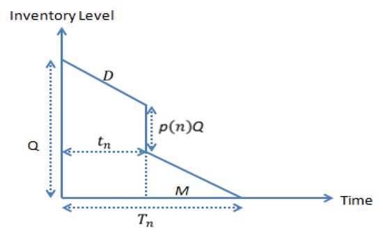
Figure 6. Inventory system for Case 2.

The retailer’s total profit for Case 2 is given as

$${\Psi }_2\left(Q\right)=\frac{\begin{array}{l}s(1-p(n))Q+vp(n)Q-k-cQ-dQ-h\left(\frac{T_n\left(1-p(n)\right)Q}{2}+\frac{Q^{2}p\left(n\right)}{\chi }\right)\\ +p{I}_{e}D{\left(M\right)}^2/2+c_s{I}_{e}p\left(n\right)Q\left(M-t_n\right)-c{I}_{p}D\hspace{0.17em}\hspace{0.17em}{T}_n{\left(T_n-M\right)}^2/2\end{array}}{T_n}$$

The retailer’s total profit per cycle is given as

$$\begin{array}{l}{\Psi }_2\left(Q\right)=sD+\frac{[vp(n)+c_s{I}_{e}p(n)(M-t_n)-(c+d)+c{I}_p(1-p(n))M]}{1-p(n)}D+\frac{D^2.M^2(p{I}_e-c{I}_P)}{2(1-p(n))Q}\\ -\frac{Q\left[h{(1-p(n))}^2\chi +2.D.P(n)+\chi c{I}_p{(1-p(n))}^2-2.D{c}_s.I_{e}p(n)\right]}{2\chi (1-p(n))}-\frac{KD}{(1-p(n))Q}\end{array}$$

(21)

To maximize the total profit per cycle for the given value of $Q$, taking the first derivative of Equation (21), we get

$$\begin{array}{l}\frac{d{\Psi }_2\left(Q\right)}{dQ}=-\frac{[vp(n)+c_s{I}_{e}p(n)(\frac{1}{\chi })]}{1-p(n)}D-\frac{D^2.M^2(p{I}_e-c{I}_P)}{2(1-p(n))Q^2}\\ -\frac{\left[h{(1-p(n))}^2\chi +2.D.P(n)+\chi c{I}_p{(1-p(n))}^2-2.D{c}_s.I_{e}p(n)\right]}{2\chi (1-p(n))}+\frac{KD}{(1-p(n))Q^2}\end{array}$$

Now, the calculation for order quantity is the same as Case 1.

$$\begin{array}{l}\mathrm{If}\frac{d{\Psi }_2{}^1\left(Q\right)}{dQ}=0=-\frac{[vp(n)+c_s{I}_{e}p(n)(\frac{1}{\chi })]}{1-p(n)}D-\frac{D^2.M^2(p{I}_e-c{I}_P)}{2(1-p(n))Q^2}\\ -\frac{\left[h{(1-p(n))}^2\chi +2.D.P(n)+\chi c{I}_p{(1-p(n))}^2-2.D{c}_s.I_{e}p(n)\right]}{2\chi (1-p(n))}+\frac{KD}{(1-p(n))Q^2}\end{array}$$

(22)

$$Q=\sqrt{\frac{\left[-\frac{D^2{M}^2(p{I}_e-c{I}_P)}{2(1-p(n))}+\frac{KD}{(1-p(n))}\right]}{\frac{[vp(n)+c_s{I}_{e}p(n)(\frac{1}{\chi })]}{1-p(n)}D+\frac{\left[\begin{array}{l}h(1-p(n))2\chi +2Dp(n)\\ +\chi c{I}_p(1-p(n))2\\ -2D{c}_s{I}_{e}p(n)\end{array}\right]}{2\chi (1-p(n))}}}$$

(23)

Taking the second derivative of Equation (21) with respect to $Q$, we get

$$\frac{d{\Psi }_2{}^2\left(Q\right)}{d{Q}^2}=\frac{D^2{M}^2(p{I}_e-c{I}_P)}{(1-p(n))Q^3}-\frac{2KD}{(1-p(n))Q^3}$$

(24)

The total profit will maximize with respect to Q when it satisfies the following $\frac{{\Psi }_2{}^2\left(Q\right)}{d{Q}^2}\le 0$.

Substituting the value of $Q$ from Equation (23) into Equation (24),

$$\frac{{\Psi }_2{}^2\left(Q\right)}{d{Q}^2}=\frac{D^2{M}^2(I_{e}p-I_{p}c)}{(1-p(n))Q^3}-\frac{2KD}{(1-p(n))Q^3}$$

(25)

We can see analytically in Appendix B that we get from Equation (16)

$$\frac{D^2{M}^2(I_{e}p-I_{p}c)}{(1-p(n))Q_1{}^3}<\frac{2KD}{(1-p(n))Q_1{}^3}$$

(26)

Finally, from Equations (25) and (26),

$$\frac{{\Psi }_1{}^2\left(Q\right)}{d{Q}^2}\le 0$$

Then, the value of $Q$ is an optimal value for the total profit, and it is represented by $Q^{\ast }$. Substituting its value into Equations (9), (10), and (20),

$$T_n=\frac{\left(1-p\left(n\right)\right)Q^{\ast }}{D}$$

(27)

$$t_n=\frac{Q^{\ast }}{\chi }$$

(28)

After putting all the values in the total profit function,

$$\begin{array}{l}{\Psi }_2\left(Q^{\ast }\right)=sD+\frac{[vp(n)+c_s{I}_{e}p(n)(M-\frac{Q^{\ast }}{\chi })-(c+d)+c{I}_p(1-p(n))M]}{1-p(n)}D+\frac{D^2{M}^2(p{I}_e-c{I}_P)}{2(1-p(n))Q^{\ast }}\\ -\frac{Q^{\ast }\left[h{(1-p(n))}^2\chi +2.DP(n)+\chi c{I}_p{(1-p(n))}^2-2D{c}_s{I}_{e}p(n)\right]}{2\chi (1-p(n))}-\frac{KD}{(1-p(n))Q^{\ast }}\end{array}$$

(29)

where

$$Q^{\ast }=\sqrt{\frac{\left[-\frac{D^2{M}^2(p{I}_e-c{I}_P)}{2(1-p(n))}+\frac{KD}{(1-p(n))}\right]}{\frac{[vp(n)+c_s{I}_{e}p(n)(\frac{1}{\chi })]}{1-p(n)}D+\frac{\left[\begin{array}{l}h(1-p(n){)}^2\chi +2Dp(n)\\ +\chi c{I}_p(1-p(n){)}^2\\ -2D{c}_s{I}_{e}p(n)\end{array}\right]}{2\chi (1-p(n))}}}$$

Case 3: $0\le t_n\le T_n\le M$.

From Figure 7, the retailer earns a profit on total income from trades up to credit period $M$ and the trades of non-good-quality items for the period $\left(M-t_n\right)$. This profit is equal to $p{I}_{e}D{\left(T_n\right)}^2/2+c_s{I}_{e}p\left(n\right)y{\hspace{0.17em}}_n\left(M-t_n\right)+p{I}_{e}D{T}_n\left(M-T_n\right)$.

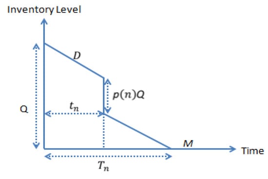
Figure 7. Inventory system for Case 3.

In this case, the retailer will not pay extra money due to credit financing.

The retailer’s total profit per cycle is equal to

$${\Psi }_3\left(Q\right)=\frac{\begin{array}{l}s(1-p(n))Q+vp(n)Q-k-cQ-dQ-h.\left(\frac{T_n\left(1-p(n)\right)Q}{2}+\frac{Q^{2}p\left(n\right)}{\chi }\right)\\ +p{I}_{e}D{\left(T_n\right)}^2/2+c_s{I}_{e}p\left(n\right)y{\hspace{0.17em}}_n\left(M-t_n\right)+p{I}_{e}D{T}_n\left(M-T_n\right)-0\end{array}}{T_n}$$

$$\begin{array}{l}{\Psi }_3(Q)=sD+vD\frac{p(n)}{1-p(n)}+\frac{I_{e}p(-p(n)+1)Q}{2}+\frac{c_s.I_{e}p(n)(M-t_n)D}{1-p(n)}-\frac{KD}{(-p(n)+1)Q}\\ -\frac{(c+d)D}{1-p(n)}-\hspace{0.17em}\frac{\hspace{0.17em}h\hspace{0.17em}Q\left[(1-p{(n)}^2\chi +2p(n)D\right]}{2(1-p(n))\chi }+p.I_{e}D.M-p.I_e(-p(n)+1)Q\end{array}$$

(30)

To maximize the total profit per cycle for the given value of $Q$, taking the first derivative of Equation (29), we get

$$\begin{array}{l}\frac{d{\Psi }_3{}^1\left(Q\right)}{dQ}=\frac{I_{e}p\hspace{0.17em}(-p(n)+1)}{2}-\frac{c_s{I}_{e}p(n)(\frac{1}{\chi })D}{1-p(n)}+\frac{KD}{(-p(n)+1)Q^2}-\frac{\hspace{0.17em}h\hspace{0.17em}\left[\begin{array}{l}{\left(1-p\left(n\right)\right)}^2\chi \\ +2p(n)D\end{array}\right]}{2(1-p(n))\chi }-p{I}_e(-p(n)+1)\end{array}$$

$$\begin{array}{l}\mathrm{If}\hspace{0.17em}\frac{d{\Psi }_3{}^1\left(Q\right)}{dQ}=0=\frac{I_{e}p\hspace{0.17em}(-p(n)+1)}{2}-\frac{c_s{I}_{e}p(n)(\frac{1}{\chi })D}{1-p(n)}+\frac{KD}{(-p(n)+1)Q^2}-\hspace{0.17em}\frac{\hspace{0.17em}h\hspace{0.17em}\left[\begin{array}{l}{\left(1-p\left(n\right)\right)}^2\chi \\ +2p(n)D\end{array}\right]}{2(1-p(n))\chi }-p{I}_e(-p(n)+1)\end{array}$$

(31)

After solving Equation (31) for $Q$, we get the value of $Q$

$$\begin{array}{l}Q=\sqrt{\frac{\frac{KD}{(-p(n)+1)}}{\frac{I_{e}p\hspace{0.17em}(-p(n)+1)}{2}-\frac{c_s{I}_{e}p(n)(\frac{1}{\chi })D}{1-p(n)}-\frac{\hspace{0.17em}h\hspace{0.17em}\left[(1-p{(n)}^2\chi +2p(n)D\right]}{2(1-p(n))\chi }-p{I}_e(-p(n)+1)}}\end{array}$$

(32)

Taking the second derivative of Equation (30) with respect to $Q$, we get (see Appendix C)

$$\frac{d{\Psi }_3{}^2\left(Q\right)}{d{Q}^2}=-\frac{2KD}{(-p(n)+1)Q^3}$$

(33)

If $Q$ is maximum, then it must be satisfied, $\frac{{\Psi }_3{}^2\left(Q\right)}{d{Q}^2}\le 0$.

The value of $Q$ from Equation (32) is substituted into Equation (33).

Finally, from Equation (33), we get

$$\frac{{\Psi }_3{}^2\left(Q\right)}{d{Q}^2}\le 0$$

Then, the value of $Q$ is an optimal value for the total profit, and it is represented by, $Q^{\ast }$. Substituting its value into Equations (9), (10), and (29),

$$T_n=\frac{\left(1-p\left(n\right)\right)Q^{*}}{D}$$

(34)

$$t_n=\frac{Q^{\ast }}{\chi }$$

(35)

$$\begin{array}{l}{\Psi }_3(Q^{\ast })=sD+vD\frac{p(n)}{1-p(n)}+\frac{I_{e}p(-p(n)+1)Q^{\ast }}{2}+\frac{c_s.I_{e}p(n)(M-t_n)D}{1-p(n)}-\frac{KD}{(-p(n)+1)Q^{\ast }}\\ -\frac{(c+d)D}{1-p(n)}-\hspace{0.17em}\frac{\hspace{0.17em}h\hspace{0.17em}{Q}^{\ast }\left[(1-p{(n)}^2\chi +2p(n)D\right]}{2(1-p(n))\chi }+p.I_{e}D.M-p.I_e(-p(n)+1)Q^{\ast }\end{array}$$

(36)

Now, the combined total profit function of the three cases is given as

$${\Psi }_{CE}\left(Q^{\ast }\right)=\left\{\begin{array}{l}{\Psi }_1\left(Q^{\ast }\right),\hspace{0.17em}\hspace{0.17em}\hspace{0.17em}\hspace{0.17em}\hspace{0.17em}\hspace{0.17em}{T}_n\ge t_n\ge M\hspace{0.17em}\hspace{0.17em}\hspace{0.17em}\hspace{0.17em}Case\hspace{0.17em}\hspace{0.17em}-\hspace{0.17em}1\hspace{0.17em}\hspace{0.17em}\\ {\Psi }_2\left(Q^{\ast }\right),\hspace{0.17em}\hspace{0.17em}\hspace{0.17em}\hspace{0.17em}\hspace{0.17em}\hspace{0.17em}\hspace{0.17em}{T}_n\ge M\ge t_n\hspace{0.17em}\hspace{0.17em}\hspace{0.17em}Case\hspace{0.17em}\hspace{0.17em}-2\hspace{0.17em}\hspace{0.17em}\\ {\Psi }_3\left(Q^{\ast }\right),\hspace{0.17em}\hspace{0.17em}\hspace{0.17em}\hspace{0.17em}\hspace{0.17em}\hspace{0.17em}\hspace{0.17em}M\ge T\ge t_n\hspace{0.17em}\hspace{0.17em}\hspace{0.17em}\hspace{0.17em}\hspace{0.17em}Case\hspace{0.17em}\hspace{0.17em}-3\hspace{0.17em}\hspace{0.17em}\end{array}\right.$$

(37)

5. Formulation of Total Profit Function under Fuzzy Environment

It is assumed that the demand rate is imprecise in nature but possible to explain with triangular fuzzy numbers because triangular fuzzy numbers are a good representation for the uncertain nature and also easy to handle. A triangular fuzzy number is used to model the demand function [39] which is given as

$$\tilde{D}\hspace{0.17em}=\left(D-{\Delta }_l{}^D,\hspace{0.17em}D,\hspace{0.17em}D+{\Delta }_h{}^D\right)$$

$$d\left(\tilde{D},0\right)=\frac{1}{4}\left(D-{\Delta }_l{}^D+2D+D+{\Delta }_h{}^D\right)=D+\frac{1}{4}{\Delta }_h{}^D-\frac{1}{4}{\Delta }_l{}^D$$

(38)

Now, the concept of the fuzzy environment is used for each case, which is given below.

5.1. Formulation of Total Profit Function under Fuzzy Environment for Case 1

Now, the fuzzification of the total profit function for Case 1 is

$$\begin{array}{l}{\tilde{\Psi }}_1\left(Q\right)=s\tilde{D}+\frac{vDp(n)}{1-p(n)}+\frac{{\tilde{D}}^2.M^2(I_{e}p-I_{p}c)}{2(1-p(n))Q}-\frac{K\tilde{D}}{(1-p(n))Q}\\ -\frac{(c+d-c_s{I}_{p}p(n).M-c.I_p(1-p(n)M)\tilde{D}}{1-p(n)}-\\ \frac{\left[h\left(\frac{{(1-p(n))}^2}{2\tilde{D}}+\frac{p(n)}{\chi }\right)+\frac{c.I_p{(1-p(n))}^2}{2\tilde{D}}+\frac{c_s{I}_{p}p(n)}{\chi }\right]Q\tilde{D}}{1-p(n)}\end{array}$$

(39)

The defuzzification of fuzzy total profit per cycle is

$$\begin{array}{l}d\left({\tilde{\Psi }}_1\left(Q\right),0\right)=sd\left(\tilde{D},0\right)+\frac{vd\left(\tilde{D},0\right)p(n)}{1-p(n)}+\frac{{\left(d\left(\tilde{D},0\right)\right)}^2{M}^2(I_{e}p-I_{p}c)}{2(1-p(n))Q}-\frac{Kd\left(\tilde{D},0\right)}{(1-p(n))Q}\\ -\frac{(c+d-c_s{I}_{p}p(n).M-c.I_p(1-p(n)M)d\left(\tilde{D},0\right)}{1-p(n)}-\\ \frac{\left[h\left(\frac{{(1-p(n))}^2}{2d\left(\tilde{D},0\right)}+\frac{p(n)}{\chi }\right)+\frac{c.I_p{(1-p(n))}^2}{2d\left(\tilde{D},0\right)}+\frac{c_s{I}_{p}p(n)}{\chi }\right]Qd\left(\tilde{D},0\right)}{1-p(n)}\end{array}$$

(40)

Substituting the value of $d\left(\tilde{D},\hspace{0.17em}0\right)$ from Equation (38) into (40), we get

$$\begin{array}{l}d\left({\tilde{\Psi }}_1\left(Q\right),0\right)={\tilde{\Psi }}_{21}\left(Q\right)=s\left(D+\frac{{\Delta }_l}{4}-\frac{{\Delta }_h}{4}\right)+\frac{v\left(D+\frac{{\Delta }_l}{4}-\frac{{\Delta }_h}{4}\right)p(n)}{1-p(n)}+\frac{{\left(\right(D+\frac{{\Delta }_l}{4}-\frac{{\Delta }_h}{4}\left)\right)}^2{M}^2(I_{e}p-I_{p}c)}{2(1-p(n))Q}\\ -\frac{K\left(D+\frac{{\Delta }_l}{4}-\frac{{\Delta }_h}{4}\right)}{(1-p(n))Q}-\frac{(c+d-c_s{I}_{p}p(n).M-c.I_p(1-p(n)M)\left(D+\frac{{\Delta }_l}{4}-\frac{{\Delta }_h}{4}\right)}{1-p(n)}-\\ \frac{\left[h\left(\frac{{(1-p(n))}^2}{2\left(D+\frac{{\Delta }_l}{4}-\frac{{\Delta }_h}{4}\right)}+\frac{p(n)}{\chi }\right)+\frac{c.I_p{(1-p(n))}^2}{2\left(D+\frac{{\Delta }_l}{4}-\frac{{\Delta }_h}{4}\right)}+\frac{c_s{I}_{p}p(n)}{\chi }\right]Q\left(D+\frac{{\Delta }_l}{4}-\frac{{\Delta }_h}{4}\right)}{1-p(n)}\end{array}$$

(41)

5.2. Formulation of Total Profit Function under Fuzzy Environment for Case 2

The fuzzification of the total profit function for Case 2 is given as

$$\begin{array}{l}{\tilde{\Psi }}_2\left(Q\right)=s\tilde{D}+\frac{[vp(n)+c_s{I}_{e}p(n)(M-t_n)-(c+d)+c{I}_p(1-p(n))M]}{1-p(n)}\tilde{D}+\frac{{\tilde{D}}^2.M^2(p{I}_e-c{I}_P)}{2(1-p(n))Q}\\ -\frac{Q\left[h{(1-p(n))}^2\chi +2.\tilde{D}.P(n)+\chi c{I}_p{(1-p(n))}^2-2.\tilde{D}{c}_s.I_{e}p(n)\right]}{2\chi (1-p(n))}-\frac{K\tilde{D}}{(1-p(n))Q}\end{array}$$

(42)

The defuzzification of fuzzy total profit per cycle from (42) is given as

$$\begin{array}{l}d\left({\tilde{\Psi }}_2\left(Q\right),0\right)=sd\left(\tilde{D},0\right)+\frac{[vp(n)+c_s{I}_{e}p(n)(M-t_n)-(c+d)+c{I}_p(1-p(n))M]}{1-p(n)}d\left(\tilde{D},0\right)\\ +\frac{{\left(d\left(\tilde{D},0\right)\right)}^2.M^2(p{I}_e-c{I}_P)}{2(1-p(n))Q}\\ -\frac{Q\left[h{(1-p(n))}^2\chi +2.\tilde{D}.P(n)+\chi c{I}_p{(1-p(n))}^2-2.d\left(\tilde{D},0\right)c_s.I_{e}p(n)\right]}{2\chi (1-p(n))}-\frac{Kd\left(\tilde{D},0\right)}{(1-p(n))Q}\end{array}$$

(43)

Substituting the value of $d\left(\tilde{D},\hspace{0.17em}0\right)$ from Equation (38) into (43), we get

$$\begin{array}{l}d\left({\tilde{\Psi }}_2\left(Q\right),0\right)={\tilde{\Psi }}_{23}\left(Q\right)=s\left(D+\frac{{\Delta }_l}{4}-\frac{{\Delta }_h}{4}\right)\\ +\frac{[vp(n)+c_s{I}_{e}p(n)(M-t_n)-(c+d)+c{I}_p(1-p(n))M]}{1-p(n)}\left(D+\frac{{\Delta }_l}{4}-\frac{{\Delta }_h}{4}\right)\\ +\frac{{\left(\left(D+\frac{{\Delta }_l}{4}-\frac{{\Delta }_h}{4}\right)\right)}^2.M^2(p{I}_e-c{I}_P)}{2(1-p(n))Q}-\frac{Q\left[\begin{array}{l}h{(1-p(n))}^2\chi +2.\left(D+\frac{{\Delta }_l}{4}-\frac{{\Delta }_h}{4}\right)P(n)\\ +\chi c{I}_p{(1-p(n))}^2\\ -2.\left(D+\frac{{\Delta }_l}{4}-\frac{{\Delta }_h}{4}\right)c_s.I_{e}p(n)\end{array}\right]}{2\chi (1-p(n))}\\ -\frac{K\left(D+\frac{{\Delta }_l}{4}-\frac{{\Delta }_h}{4}\right)}{(1-p(n))Q}\end{array}$$

(44)

5.3. Formulation of Total Profit Function under Fuzzy Environment for Case 3

The fuzzification of the total profit function for Case 3 is given as

$$\begin{array}{l}{\tilde{\Psi }}_3(Q)=s\tilde{D}+v.\tilde{D}\frac{p(n)}{1-p(n)}+\frac{I_{e}p(-p(n)+1)Q}{2}+\frac{c_s.I_{e}p(n)(M-t_n)\tilde{D}}{1-p(n)}-\frac{K\tilde{D}}{(-p(n)+1)Q}\\ -\frac{(c+d)\tilde{D}}{1-p(n)}-\hspace{0.17em}\frac{\hspace{0.17em}h\hspace{0.17em}Q\left[(1-p{(n)}^2\chi +2p(n)\tilde{D}\right]}{2(1-p(n))\chi }+p.I_e\tilde{D}.M-p.I_e(-p(n)+1)Q\\ \hspace{0.17em}\end{array}$$

(45)

The defuzzification of fuzzified total profit per cycle is given as

$$\begin{array}{l}{\tilde{\Psi }}_3(Q)=sd\left(\tilde{D},0\right)+vd\left(\tilde{D},0\right)\frac{p(n)}{1-p(n)}+\frac{I_{e}p(-p(n)+1)Q}{2}+\frac{c_s.I_{e}p(n)(M-t_n)d\left(\tilde{D},0\right)}{1-p(n)}-\frac{Kd\left(\tilde{D},0\right)}{(-p(n)+1)Q}\\ -\frac{(c+d)d\left(\tilde{D},0\right)}{1-p(n)}-\hspace{0.17em}\frac{\hspace{0.17em}h\hspace{0.17em}Q\left[(1-p{(n)}^2\chi +2p(n)d\left(\tilde{D},0\right)\right]}{2(1-p(n))\chi }+p.I_{e}d\left(\tilde{D},0\right)M-p.I_e(-p(n)+1)Q\\ \hspace{0.17em}\end{array}$$

(46)

Substituting the value of $d\left(\tilde{D},\hspace{0.17em}0\right)$ from Equation (38) into (46), we get

$$\begin{array}{l}d\left({\tilde{\Psi }}_3\left(Q,\hspace{0.17em}0\right)\right)={\tilde{\Psi }}_{23}\left(Q\right)=\\ s\left(D+\frac{{\Delta }_l}{4}-\frac{{\Delta }_h}{4}\right)+v.\left(D+\frac{{\Delta }_l}{4}-\frac{{\Delta }_h}{4}\right)\frac{p(n)}{1-p(n)}+\frac{I_{e}p(-p(n)+1)Q}{2}\\ +\frac{c_s.I_{e}p(n)(M-t_n)\left(D+\frac{{\Delta }_l}{4}-\frac{{\Delta }_h}{4}\right)}{1-p(n)}-\frac{K\left(D+\frac{{\Delta }_l}{4}-\frac{{\Delta }_h}{4}\right)}{(-p(n)+1)Q}-\frac{(c+d)\left(D+\frac{{\Delta }_l}{4}-\frac{{\Delta }_h}{4}\right)}{1-p(n)}\\ -\hspace{0.17em}\frac{\hspace{0.17em}h\hspace{0.17em}Q\left[(1-p{(n)}^2\chi +2p(n)\left(D+\frac{{\Delta }_l}{4}-\frac{{\Delta }_h}{4}\right)\right]}{2(1-p(n))\chi }+p.I_e\left(D+\frac{{\Delta }_l}{4}-\frac{{\Delta }_h}{4}\right)M-p.I_e(-p(n)+1)Q\end{array}$$

(47)

Now, the total fuzzy profit functions of the three cases are combined, which is given as

$${\tilde{\Psi }}_{GF}\left(Q\right)=\left\{\begin{array}{l}{\tilde{\Psi }}_{21}\left(Q\right),\hspace{0.17em}\hspace{0.17em}\hspace{0.17em}\hspace{0.17em}\hspace{0.17em}\hspace{0.17em}{T}_n\ge t_n\ge M\hspace{0.17em}\hspace{0.17em}\hspace{0.17em}\hspace{0.17em}Case\hspace{0.17em}\hspace{0.17em}-\hspace{0.17em}1\hspace{0.17em}\hspace{0.17em}\\ {\tilde{\Psi }}_{22}\left(Q\right),\hspace{0.17em}\hspace{0.17em}\hspace{0.17em}\hspace{0.17em}\hspace{0.17em}\hspace{0.17em}\hspace{0.17em}{T}_n\ge M\ge t_n\hspace{0.17em}\hspace{0.17em}\hspace{0.17em}Case\hspace{0.17em}\hspace{0.17em}-2\hspace{0.17em}\hspace{0.17em}\\ {\tilde{\Psi }}_{32}\left(Q\right),\hspace{0.17em}\hspace{0.17em}\hspace{0.17em}\hspace{0.17em}\hspace{0.17em}\hspace{0.17em}\hspace{0.17em}M\ge T\ge t_n\hspace{0.17em}\hspace{0.17em}\hspace{0.17em}\hspace{0.17em}\hspace{0.17em}Case\hspace{0.17em}\hspace{0.17em}-3\hspace{0.17em}\hspace{0.17em}\end{array}\right.$$

(48)

Now, we move to the cloudy fuzzy environment with the help of the fuzzy environment, which is already given in Section 2. The formulation of the total profit function for each case under the cloudy environment is given in Section 5 briefly.

6. Formulation of Total Fuzzy Profit Function under Cloudy Fuzzy Environment

As mentioned above, the nature of the demand rate is a cloudy fuzzy number, and the ordered lot is dependent on the demand rate. The fuzzified maximization model is given below case wise. Now, using Equation (9) for Case 1

$$\begin{array}{l}\mathrm{Maximize}\hspace{0.17em}{\tilde{\Psi }}_1\left(Q\right)=s\tilde{D}+\frac{vDp(n)}{1-p(n)}+\frac{{\tilde{D}}^2.M^2(I_{e}p-I_{p}c)}{2(1-p(n))Q}-\frac{K\tilde{D}}{(1-p(n))Q}\\ -\frac{(c+d-c_s{I}_{p}p(n).M-c.I_p(1-p(n)M)\tilde{D}}{1-p(n)}-\\ \frac{\left[h\left(\frac{{(1-p(n))}^2}{2\tilde{D}}+\frac{p(n)}{\chi }\right)+\frac{c.I_p{(1-p(n))}^2}{2\tilde{D}}+\frac{c_s{I}_{p}p(n)}{\chi }\right]Q\tilde{D}}{1-p(n)}\\ \mathrm{Subjected}\hspace{0.17em}\mathrm{to}\hspace{0.17em}\hspace{0.17em}\tilde{Q}=\frac{\tilde{D}{T}_n}{1-p\left(n\right)}\end{array}$$

(49)

Further, using Equation (12) for Case 2,

$$\begin{array}{l}\mathrm{Maximize}\hspace{0.17em}{\tilde{\Psi }}_2\left(Q\right)=s\tilde{D}+\frac{[vp(n)+c_s{I}_{e}p(n)(M-t_n)-(c+d)+c{I}_p(1-p(n))M]}{1-p(n)}\tilde{D}+\\ \frac{{\tilde{D}}^2.M^2(p{I}_e-c{I}_P)}{2(1-p(n))Q}-\frac{Q\left[h{(1-p(n))}^2\chi +2.\tilde{D}.P(n)+\chi c{I}_p{(1-p(n))}^2-2.\tilde{D}{c}_s.I_{e}p(n)\right]}{2\chi (1-p(n))}\\ -\frac{K\tilde{D}}{(1-p(n))Q}\\ \mathrm{Subjected}\hspace{0.17em}\mathrm{to}\hspace{0.17em}\hspace{0.17em}\tilde{Q}=\frac{\tilde{D}{T}_n}{1-p\left(n\right)}\end{array}$$

(50)

Similarly, using Equation (15) for Case 3

$$\begin{array}{l}\mathrm{Maximize}\hspace{0.17em}{\tilde{\Psi }}_3(Q)=s\tilde{D}+v.\tilde{D}\frac{p(n)}{1-p(n)}+\frac{I_{e}p(-p(n)+1)Q}{2}+\frac{c_s.I_{e}p(n)(M-t_n)\tilde{D}}{1-p(n)}-\frac{K\tilde{D}}{(-p(n)+1)Q}\\ -\frac{(c+d)\tilde{D}}{1-p(n)}-\hspace{0.17em}\frac{\hspace{0.17em}h\hspace{0.17em}Q\left[(1-p{(n)}^2\chi +2p(n)\tilde{D}\right]}{2(1-p(n))\chi }+p.I_e\tilde{D}.M-p.I_e(-p(n)+1)Q\\ \mathrm{Subjected}\hspace{0.17em}\mathrm{to}\hspace{0.17em}\hspace{0.17em}\tilde{Q}=\frac{\tilde{D}{T}_n}{1-p\left(n\right)}\end{array}$$

(51)

Now, the membership function of the demand rate $D$ is given as

$$f\left(\tilde{D},T_n\right)=\left\{\begin{array}{l}0\hspace{0.17em}\hspace{0.17em}\hspace{0.17em}\hspace{0.17em}\hspace{0.17em}\hspace{0.17em}\hspace{0.17em}\hspace{0.17em}\hspace{0.17em}\hspace{0.17em}\hspace{0.17em}\hspace{0.17em}\mathrm{if}\hspace{0.17em}\hspace{0.17em}D⟨D_2\left(1-\frac{\rho }{1+T_n}\right)\hspace{0.17em}\hspace{0.17em}\mathrm{and}\hspace{0.17em}\hspace{0.17em}\hspace{0.17em}D⟩\hspace{0.17em}{D}_2\left(1+\frac{\sigma }{1+T_n}\right)\\ \frac{D-D_2\left(1-\frac{\rho }{1+T_n}\right)}{\frac{\rho D_2}{1+T_n}}\hspace{0.17em}\hspace{0.17em}\mathrm{if}\hspace{0.17em}\hspace{0.17em}\hspace{0.17em}\hspace{0.17em}\hspace{0.17em}{D}_2\left(1-\frac{\rho }{1+T_n}\right)\le D\le D_2\\ \frac{D_2\left(1+\frac{\sigma }{1+T_n}\right)-D}{\frac{\sigma D_2}{1+T_n}}\hspace{0.17em}\hspace{0.17em}\mathrm{if}\hspace{0.17em}\hspace{0.17em}\hspace{0.17em}\hspace{0.17em}\hspace{0.17em}\hspace{0.17em}{D}_2\le D\le D_2\left(1+\frac{\sigma }{1+T_n}\right)\end{array}\right.$$

(52)

The membership function of the demand rate is given as

$$f\left(\tilde{Q},T_n\right)=\left\{\begin{array}{l}0\mathrm{if}\hspace{0.17em}\frac{\left(1-p\left(n\right)\right)Q}{T_n}⟨D_2\left(1-\frac{\rho }{1+T_n}\right)\mathrm{and}\frac{\left(1-p\left(n\right)\right)Q}{T_n}⟩\hspace{0.17em}{D}_2\left(1+\frac{\sigma }{1+T_n}\right)\\ \frac{\frac{\left(1-p\left(n\right)\right)Q}{T_n}-D_2\left(1-\frac{\rho }{1+T_n}\right)}{\frac{\rho D_2}{1+T_n}}\mathrm{if}{D}_2\left(1-\frac{\rho }{1+T_n}\right)\le \frac{\left(1-p\left(n\right)\right)Q}{T_n}\le D_2\\ \frac{D_2\left(1+\frac{\sigma }{1+T_n}\right)-\frac{\left(1-p\left(n\right)\right)Q}{T_n}}{\frac{\sigma D_2}{1+T_n}}\mathrm{if}{D}_2\le \frac{\left(1-p\left(n\right)\right)Q}{T_n}\le D_2\left(1+\frac{\sigma }{1+T_n}\right)\end{array}\right.$$

$$f\left(\tilde{Q},T_n\right)=\left\{\begin{array}{l}0\mathrm{if}\hspace{0.17em}Q⟨T_n{D}_2\left(1-\frac{\rho }{1+T_n}\right)\raisebox{1ex}{$1$}\!\left/ \!\raisebox{-1ex}{$1-p\left(n\right)$}\right.\mathrm{and}Q⟩\hspace{0.17em}{T}_n{D}_2\left(1+\frac{\sigma }{1+T_n}\right)\raisebox{1ex}{$1$}\!\left/ \!\raisebox{-1ex}{$1-p\left(n\right)$}\right.\\ \frac{Q-T_n{D}_2\left(1-\frac{\rho }{1+T_n}\right)\raisebox{1ex}{$1$}\!\left/ \!\raisebox{-1ex}{$1-p\left(n\right)$}\right.}{\frac{\rho D_2}{1+T_n}}\mathrm{if}{D}_2\left(1-\frac{\rho }{1+T_n}\right)\le \frac{\left(1-p\left(n\right)\right)Q}{T_n}\le D_2\\ \frac{T_n{D}_2\left(1+\frac{\sigma }{1+T_n}\right)\raisebox{1ex}{$1$}\!\left/ \!\raisebox{-1ex}{$1-p\left(n\right)$}\right.-Q}{\frac{\sigma D_2}{1+T_n}}\mathrm{if}{T}_n{D}_2\raisebox{1ex}{$1$}\!\left/ \!\raisebox{-1ex}{$1-p\left(n\right)$}\right.\le Q\le T_n{D}_2\left(1+\frac{\sigma }{1+T_n}\right)\raisebox{1ex}{$1$}\!\left/ \!\raisebox{-1ex}{$1-p\left(n\right)$}\right.\end{array}\right.$$

(53)

Moreover, the $\alpha -\mathrm{cuts}$ of $f\left({\tilde{D},T}_n\right)$ and $f\left({\tilde{Q},T}_n\right)$ are obtained by using Equations (33) and (34), and they can be put as the left and right cloudy triangular fuzzy numbers

$$\left[D_2\left(1-\frac{\rho }{1+T_n}\right)+\frac{\alpha \rho D_2}{1+T_n},\hspace{0.17em}{D}_2,\hspace{0.17em}{D}_2\left(1+\frac{\sigma }{1+T_n}\right)-\frac{\alpha \sigma D_2}{1+T_n}\right]$$

and

$$\left[\frac{D_2{T}_n}{1-p\left(n\right)}\left(1-\frac{\rho }{1+T_n}\right)+\frac{\alpha \rho T_n{D}_2}{1+T_n},\hspace{0.17em}\frac{D_2{T}_n}{1-p\left(n\right)},\hspace{0.17em}\frac{D_2{T}_n}{1-p\left(n\right)}\left(1+\frac{\sigma }{1+T_n}\right)-\frac{\alpha \sigma D_2}{1+T_n}\right]$$

respectively.

Now, the index value of $\tilde{Q}$ and $\tilde{D}$ is obtained as

$$I\left(\tilde{Q}\right)=\frac{1}{2\tau }{\displaystyle {\int }_{T_n=0}^{T_n=\tau }}{\displaystyle {\int }_{\alpha =0}^{\alpha =1}\left[\frac{D_2{T}_n}{1-p\left(n\right)}\left(1-\frac{\rho }{1+T_n}\right)+\frac{\alpha \rho T_n{D}_2}{1+T_n}+\hspace{0.17em}\frac{D_2{T}_n}{1-p\left(n\right)}\left(1+\frac{\sigma }{1+T_n}\right)-\frac{\alpha \sigma D_2}{1+T_n}\right]}d\alpha d{T}_n$$

(54)

From Equation (54), we can write it in the simplest form

$$I\left(\tilde{Q}\right)=\frac{D_2\tau }{2\left(1-p\left(n\right)\right)}-\frac{D_2\left(\rho -\sigma \right)}{4\left(1-p\left(n\right)\right)}\left[1-\frac{\log |1+\tau |}{\tau }\right]$$

(55)

Now, we can find out the index value demand rate

$$I\left(\tilde{D}\right)=\frac{D_2}{2\tau }{\displaystyle {\int }_{T_n=0}^{T_n=\tau }}{\displaystyle {\int }_{\alpha =0}^{\alpha =1}\left[\left(1-\frac{\rho }{1+T_n}\right)+\frac{\alpha \rho }{1+T_n}+\hspace{0.17em}\left(1+\frac{\sigma }{1+T_n}\right)-\frac{\alpha \sigma }{1+T_n}\right]}d\alpha d{T}_n$$

(56)

$$I\left(\tilde{D}\right)=D_2+\frac{D_2\left(\rho -\sigma \right)}{4}\left[1-\frac{\log |1+\tau |}{\tau }\right]$$

(57)

The index value of the fuzzy profit objective function for Case 1 is

$$\begin{array}{l}I\left({\tilde{\Psi }}_1\left(Q\right)\right)=sI\left(\tilde{D}\right)+\frac{vI\left(\tilde{D}\right)p(n)}{1-p(n)}+\frac{{\left(I\left(\tilde{D}\right)\right)}^2.M^2(I_{e}p-I_{p}c)}{2(1-p(n))I\left(\tilde{Q}\right)}-\frac{KI\left(\tilde{D}\right)}{(1-p(n))I\left(\tilde{Q}\right)}\\ -\frac{(c+d-c_s{I}_{p}p(n).M-c.I_p(1-p(n)M)I\left(\tilde{D}\right)}{1-p(n)}-\\ \frac{\left[h\left(\frac{{(1-p(n))}^2}{2I\left(\tilde{D}\right)}+\frac{p(n)}{\chi }\right)+\frac{c.I_p{(1-p(n))}^2}{2I\left(\tilde{D}\right)}+\frac{c_s{I}_{p}p(n)}{\chi }\right]I\left(\tilde{Q}\right)I\left(\tilde{D}\right)}{1-p(n)}\end{array}$$

(58)

The index value of the fuzzy profit objective function for Case 2:

$$\begin{array}{l}I\left({\tilde{\Psi }}_2\left(Q\right)\right)=sI\left(\tilde{D}\right)+\frac{[vp(n)+c_s{I}_{e}p(n)(M-t_n)-(c+d)+c{I}_p(1-p(n))M]}{1-p(n)}I\left(\tilde{D}\right)+\frac{{\left(I\left(\tilde{D}\right)\right)}^2.M^2(p{I}_e-c{I}_P)}{2(1-p(n))I\left(\tilde{Q}\right)}\\ -\frac{I\left(\tilde{Q}\right)\left[h{(1-p(n))}^2\chi +2I\left(\tilde{D}\right).P(n)+\chi c{I}_p{(1-p(n))}^2-2.I\left(\tilde{D}\right)c_s.I_{e}p(n)\right]}{2\chi (1-p(n))}-\frac{KI\left(\tilde{D}\right)}{(1-p(n))I\left(\tilde{Q}\right)}\end{array}$$

(59)

The index value of the fuzzy profit objective function for Case 3:

$$\begin{array}{l}I\left({\tilde{\Psi }}_3\left(Q\right)\right)=sI\left(\tilde{D}\right)+vI\left(\tilde{D}\right)\frac{p(n)}{1-p(n)}+\frac{I_{e}p(-p(n)+1)I\left(\tilde{Q}\right)}{2}+\frac{c_s.I_{e}p(n)(M-t_n)I\left(\tilde{D}\right)}{1-p(n)}\\ -\frac{KI\left(\tilde{D}\right)}{(-p(n)+1)I\left(\tilde{Q}\right)}-\frac{(c+d)I\left(\tilde{D}\right)}{1-p(n)}-\hspace{0.17em}\frac{\hspace{0.17em}hI\left(\tilde{Q}\right)\left[(1-p{(n)}^2\chi +2p(n)I\left(\tilde{D}\right)\right]}{2(1-p(n))\chi }\\ +p.I_{e}I\left(\tilde{D}\right)M-p.I_e(-p(n)+1)I\left(\tilde{Q}\right)\end{array}$$

(60)

The combined form of the fuzzy total cost objective function under the cloudy fuzzy environment from Equations (58) to (60):

$$I\left(\tilde{\Psi }\left(Q\right)\right)=\left\{\begin{array}{l}I\left({\tilde{\Psi }}_1\left(Q\right)\right),\hspace{0.17em}\hspace{0.17em}\hspace{0.17em}\hspace{0.17em}\hspace{0.17em}\hspace{0.17em}{T}_n\ge t_n\ge M\hspace{0.17em}\hspace{0.17em}\hspace{0.17em}\hspace{0.17em}Case\hspace{0.17em}\hspace{0.17em}-\hspace{0.17em}1\hspace{0.17em}\hspace{0.17em}\\ I\left({\tilde{\Psi }}_2\left(Q\right)\right),\hspace{0.17em}\hspace{0.17em}\hspace{0.17em}\hspace{0.17em}\hspace{0.17em}\hspace{0.17em}\hspace{0.17em}{T}_n\ge M\ge t_n\hspace{0.17em}\hspace{0.17em}\hspace{0.17em}Case\hspace{0.17em}\hspace{0.17em}-2\hspace{0.17em}\hspace{0.17em}\\ I\left({\tilde{\Psi }}_3\left(Q\right)\right),\hspace{0.17em}\hspace{0.17em}\hspace{0.17em}\hspace{0.17em}\hspace{0.17em}\hspace{0.17em}\hspace{0.17em}M\ge T\ge t_n\hspace{0.17em}\hspace{0.17em}\hspace{0.17em}\hspace{0.17em}\hspace{0.17em}Case\hspace{0.17em}\hspace{0.17em}-3\hspace{0.17em}\hspace{0.17em}\end{array}\right.$$

(61)

In the next section, we will find the solutions to the objective functions.

7. Solution Method

For maximum total profit $\frac{d{\Psi }_i\left(Q\right)}{dQ}=0,\mathrm{where}\hspace{0.17em}i=1,2\hspace{0.17em}\mathrm{and}\hspace{0.17em}3\hspace{0.17em}\mathrm{for}\hspace{0.17em}\mathrm{each}\hspace{0.17em}\mathrm{cases},$ we obtained $Q=Q_i$ by using the Mathematica tool, the value of $Q=Q_i$ (supposed), and the value of the second derivative $\frac{d^2{\Psi }_i\left(Q\right)}{d{Q}^2}$ from Equation (17). The value of $Q=Q_i$ is substituted into $\frac{d^2{\Psi }_i\left(Q\right)}{d{Q}^2}$. If the value of $\frac{d^2{\Psi }_i\left(Q_i\right)}{d{Q}^2}\le 0,$ then $Q=Q_i$ is the optimal value of $Q$ and represented by $Q^{\ast }$. The calculations of the first and second derivatives are defined in the appendix briefly. The first and second derivatives functions are very complicated. The concavity of the profit functions is shown graphically for all cases in Figure 7.

7.1. Algorithm

An algorithm was followed, which is defined by [37] for finding the best case out of three cases.

Step 1: Insert all inventory parameters that are known $\left[D,\hspace{0.17em}{I}_e,I_p,p,d,b,k,h,n,,p\left(n\right),M,p,\chi \right]$ into Equations (12), (13), and (15).

Step 2: Now, calculate $Q^{\ast }=Q_1$ with the help of the solution method and substitution into Equations (9) and (10) to find out $T_n$ and $t_n$. If $0\le M\le t_n\le T_n$, then find out the retailer’s profit with respect to Case 1 from Equation (12).

Step 3: Now, calculate $Q^{\ast }=Q_1$ with the help of the solution method and substitution into Equations (9) and (10) to find out $Q^{\ast }=Q_1$ and $t_n$. If $0\le t_n\le M\le T_n$, then find out the retailer’s profit with respect to Case 2 from Equation (13).

Step 4: Now, calculate $Q^{\ast }=Q_1$ with the help of the solution method and substitution into Equations (9) and (10) to find out $T_n$ and $t_n$. If $0\le t_n\le T_n\le M$, then find out the retailer’s profit with respect to Case 3 from Equation (15).

Step 5: In this stage, compare all the cases and determine the best case. Get the optimal order quantity on which the profit is maximized.

Similarly, the above algorithm can be used in a similar way for the fuzzy environment section.

7.2. Inventory Model

7.2.1. Numerical Example for Crisp Model

All the inventory parameters are taken from [22] for this proposed model,

$D=5000\hspace{0.17em}units\hspace{0.17em}per\hspace{0.17em}year,\hspace{0.17em}\lambda =\mathrm{175,000}\hspace{0.17em}units\hspace{0.17em}per\hspace{0.17em}year,p=\text{\$}50\hspace{0.17em}per\hspace{0.17em}unit,\hspace{0.17em}$

$C_p=\text{\$}25\hspace{0.17em}per\hspace{0.17em}unit,h=\text{\$}5 per unit per year,hhh\hspace{0.17em}{I}_e=0.10\hspace{0.17em}per\hspace{0.17em}year,I_p=0.12\hspace{0.17em}per\hspace{0.17em}year,n=5,$

$p\left(n\right)=0.039\hspace{0.17em},M=0.054 year, d=\text{\$}0.5\hspace{0.17em}per\hspace{0.17em}unit,$

$T_n{}^{*}=0.069\hspace{0.17em}year,\hspace{0.17em}{t}_n{}^{*}=0.002\hspace{0.17em}year,\hspace{0.17em}{Q}^{*}=363\hspace{0.17em}unit,\hspace{0.17em}{\Psi }_2\left(Q^{*}\right)=\text{\$}119,662$

7.2.2. Numerical Example for Cloudy Fuzzy Model

$D=5000\hspace{0.17em}units\hspace{0.17em}per\hspace{0.17em}year,\tilde{D}=\left(50000 \left(1-\rho \right),\hspace{0.17em}50000,\hspace{0.17em}50000\left(1+\sigma \right)\right),\hspace{0.17em}\lambda =175000\hspace{0.17em}units\hspace{0.17em}per\hspace{0.17em}year,$

$p=\text{\$}\hspace{0.17em}50\hspace{0.17em}per\hspace{0.17em}unit,\hspace{0.17em}d=\text{\$}\hspace{0.17em}0.5\hspace{0.17em}per\hspace{0.17em}unit,\hspace{0.17em}{C}_p=\text{\$}25\hspace{0.17em}per\hspace{0.17em}unit,h=\text{\$}5/unit/year,\hspace{0.17em}{I}_e=0.10\hspace{0.17em}per\hspace{0.17em}year,$

$I_p=0.12\hspace{0.17em}per\hspace{0.17em}year,n=5,p\left(n\right)=0.039\rho =0.4,\sigma =0.3,\hspace{0.17em}M=0.054 year, b=0.7932,\mathrm{we} \mathrm{got}$

$T_n{}^{*}=0.1654 year,\hspace{0.17em}{t}_n{}^{*}=0.002\hspace{0.17em}year,\hspace{0.17em}{Q}^{*}=353\hspace{0.17em}unit\hspace{0.17em}\mathrm{and}\hspace{0.17em}I\left(\hspace{0.17em}{\tilde{\Psi }}_2\left(T_n{}^{*}\right)\right)=\text{\$}123,905$

From Table 2, it can be studied that the order quantity is less, but the cycle length and total profit are more in the cloudy fuzzy environment as compared to the crisp and fuzzy environments.

Table 2. Comparison of cycle length, order quantity, and total profit function under different environments.

Model	${\mathit{T}}_{\mathit{n}}{}^{\ast } \left(\mathbf{Days}\right)$	${\mathit{Q}}^{\ast }$	Total Profit Function ($)
Crisp	25	363	119,962
General fuzzy	24	368	122,332
Cloudy fuzzy	61	353	123,905

8. Managerial Insight

Managerial insight is a vital explanation for the impact of various parameters on the inventory model. The major effects of trade-credit financing policy on batch size and total profit have been determined. Table 3, Table 4, Table 5, Table 6, Table 7, Table 8, Table 9, Table 10, Table 11 and Table 12 are given below with the data determined from the inventory model by varying various parameters.

Table 3. Impact of number of shipments on screening time, cycle time, lot size, and total profit.

Number of Shipments $\left(\mathit{n}\right)$	Inspection Time (Year) ${\mathit{t}}_{\mathit{n}}$	Cycle Length (Year) ${\mathit{T}}_{\mathit{n}}$	Lot Size $\mathit{Q}$ (Units)	Retailer’s Total Profit ${\mathbf{\Psi }}_2\left(\mathit{Q}\right) \left(\text{\$}\right)$	$\mathbf{CI}=\frac{\mathbf{log}\left(1+\mathit{T}\right)}{\mathit{T}}$
1	0.002	0.1654	352	123,847	0.4019
2	0.002	0.1654	356	123,851	0.4019
3	0.002	0.1654	354	123,858	0.4019
4	0.002	0.1654	353	123,873	0.4019
5	0.002	0.1654	353	123,905	0.4019
6	0.002	0.1654	353	123,870	0.4019
7	0.002	0.1654	353	124,089	0.4019
8	0.002	0.1654	353	124,270	0.4019
9	0.002	0.1654	353	124,501	0.4019
10	0.002	0.1654	353	124,707	0.4019

Table 4. Impact of learning rate on screening time, cycle time, lot size, and total profit.

Learning Rate $\mathit{b}$	Inspection Time ${\mathit{t}}_{\mathit{n}} \left(\mathbf{Year}\right)$	Cycle Time ${\mathit{T}}_{\mathit{n}} \left(\mathbf{Year}\right)$	Lot Size $\mathit{Q}$ (Units)	Retailer’s Total Profit ${\mathbf{\Psi }}_2\left(\mathit{Q}\right) \left(\text{\$}\right)$	$\mathbf{CI}=\frac{\mathbf{log}\left(1+\mathit{T}\right)}{\mathit{T}}$
0.79	0.002	0.1654	353	123,905	0.4019
0.90	0.002	0.1655	351	123,944	0.4019
1.00	0.002	0.1655	351	123,999	0.4019
1.20	0.002	0.1655	351	124,186	0.4019
1.30	0.002	0.1655	351	124,317	0.4019
2.50	0.002	0.1655	339	125,007	0.4019
2.90	0.002	0.1655	339	125,011	0.4019
3.90	0.002	0.1655	339	125,011	0.4019

Table 5. Effect of cloudy parameters on screening time, cycle time, lot size, and index value of total profit.

Cloud Parameter $\mathit{\rho }\left(0<\mathit{\rho }<1\right)$	Cloud Parameter $\mathit{\sigma }\hspace{0.17em}\left(0<\mathit{\sigma }<1\right)$	Cycle Time ${\mathit{T}}_{\mathit{n}} \left(\mathbf{Year}\right)$	Lot Size $\mathit{Q}$ (Units)	Retailer’s Total Profit ${\mathbf{\Psi }}_2\left(\mathit{Q}\right) \left(\text{\$}\right)$	$\mathbf{CI}=\frac{\mathbf{log}\left(1+\mathit{T}\right)}{\mathit{T}}$
0.2	0.1	0.1654	353	123,905	0.4019
0.3	0.2	0.1654	353	123,905	0.4019
0.4	0.3	0.1554	353	123,905	0.4019
0.5	0.4	0.1654	353	123,905	0.4019
0.6	0.5	0.1654	353	123,905	0.4019
0.9	0.8	0.1681	296	124,328	0.4014
0.99	0.81	0.1866	343	127,278	0.3982

Table 6. Effect of credit period under impact of learning on screening rate, cycle time, and lot size and index value of total profit.

Credit Period $\mathit{M}$ (Year)	Inspection Time ${\mathit{t}}_{\mathit{n}} \left(\mathbf{Year}\right)$	Cycle Time ${\mathit{T}}_{\mathit{n}} \left(\mathbf{Year}\right)$	Lot Size $\mathit{Q}$ (Units)	Retailer’s Total Profit ${\mathbf{\Psi }}_2\left(\mathit{Q}\right) \left(\text{\$}\right)$	$\mathbf{CI}=\frac{\mathbf{log}\left(1+\mathit{T}\right)}{\mathit{T}}$
0.013	0.002	0.1966	432	123,365	0.3664
0.027	0.002	0.1916	420	123,475	0.3973
0.041	0.002	0.1816	394	123,650	0.3990
0.054	0.002	0.1654	352	123,905	0.4019
0.068	0.001	0.1357	276	124,278	0.4042

Table 7. Impact of holding cost on order quantity, cycle time, cloudy impact, and total profit.

Holding Cost $\mathit{h}$	Cloudy Impact $\frac{\mathbf{log}\left(1+\mathit{T}\right)}{\mathit{T}}$	Cycle Time ${\mathit{T}}_{\mathit{n}} \left(\mathbf{Year}\right)$	Order Quantity $\mathit{Q}$ (Units)	Retailer’s Total Profit ${\mathbf{\Psi }}_2\left(\mathit{Q}\right) \left(\text{\$}\right)$
1	0.3843	0.2710	625	124,778
2	0.3915	0.2260	508	124,508
3	0.3961	0.1983	436	124,281
4	0.3994	0.1793	387	124,083
5	0.4019	0.1654	352	123,905

Table 8. Impact of screening cost on order quantity, cycle time, cloudy impact, and total profit.

Screening Cost $\mathit{d}$	Cloudy Impact $\frac{\mathbf{log}\left(1+\mathit{T}\right)}{\mathit{T}}$	Cycle Time ${\mathit{T}}_{\mathit{n}} \left(\mathbf{Year}\right)$	Order Quantity $\mathit{Q}$ (Units)	Retailer’s Total Profit ${\mathbf{\Psi }}_2\left(\mathit{Q}\right) \left(\text{\$}\right)$
0.1	0.4019	0.1654	352	126,057
0.2	0.4019	0.1654	352	125,519
0.3	0.4019	0.1654	352	124,981
0.4	0.4019	0.1654	352	124,443
0.5	0.4019	0.1654	352	123,905

Table 9. Impact of ordering cost on order quantity, cycle time, cloudy impact, and total profit.

Ordering Cost $\mathit{K} \left(\text{\$}\right)$	Cloudy Impact $\frac{\mathbf{log}\left(1+\mathit{T}\right)}{\mathit{T}}$	Cycle Time ${\mathit{T}}_{\mathit{n}} \left(\mathbf{Year}\right)$	Order Quantity $\mathit{Q}$ (Units)	Retailer’s Total Profit ${\mathbf{\Psi }}_2\left(\mathit{Q}\right) \left(\text{\$}\right)$
50	0.4070	0.1369	278	124,817
75	0.4070	0.1369	278	124,335
100	0.4019	0.1654	352	123,905
150	0.9939	0.2113	470	123,252
200	0.3881	0.2469	562	122,731

Table 10. Impact of purchase cost on order quantity, cycle time, cloudy impact, and total profit.

Unit Cost $\mathit{c} \left(\text{\$}\right)$	Cloudy Impact $\frac{\mathbf{log}\left(1+\mathit{T}\right)}{\mathit{T}}$	Cycle Time ${\mathit{T}}_{\mathit{n}} \left(\mathbf{Year}\right)$	Order Quantity $\mathit{Q}$ (Units)	Retailer’s Total Profit ${\mathbf{\Psi }}_2\left(\mathit{Q}\right) \left(\text{\$}\right)$
5	0.4025	0.1616	342	231,506
10	0.4024	0.1626	344	204,605
15	0.4022	0.1635	347	177,705
20	0.4020	0.1645	349	150,805
25	0.4019	0.1654	352	123,905

Table 11. Impact of selling cost on order quantity, cycle time, cloudy impact, and total profit.

Unit Cost for Good Quality Items $\mathit{P} \left(\text{\$}\right)$	Cloudy Impact $\frac{\mathbf{log}\left(1+\mathit{T}\right)}{\mathit{T}}$	Cycle Time ${\mathit{T}}_{\mathit{n}} \left(\mathbf{Year}\right)$	Order Quantity $\mathit{Q}$ (Units)	Retailer’s Total Profit ${\mathbf{\Psi }}_2\left(\mathit{Q}\right) \left(\text{\$}\right)$
20	0.3982	0.1862	405	20,184
30	0.3982	0.1862	405	20,184
40	0.4002	0.1759	379	72,039
50	0.4019	0.1654	353	123,905
60	0.4038	0.1547	324	175,741

Table 12. Impact of salvage price on order quantity, cycle time, cloudy impact, and total profit.

Unit Cost for Defective Quality Items ${\mathit{c}}_{\mathit{s}}$	Cloudy Impact $\frac{\mathbf{log}\left(1+\mathit{T}\right)}{\mathit{T}}$	Cycle Time ${\mathit{T}}_{\mathit{n}} \left(\mathbf{Year}\right)$	Order Quantity $\mathit{Q}$ (Units)	Retailer’s Total Profit ${\mathbf{\Psi }}_2\left(\mathit{Q}\right) \left(\text{\$}\right)$
10	0.4018	0.1655	352	120,818
20	0.4018	0.1655	353	123,905
30	0.4018	0.1655	353	125,963

9. Sensitivity Analysis

Sensitivity analysis is performed to know the robustness of the model on the affected parameters.

9.1. Impact of Shipment

From Table 3 and Figure 8, it is found that if the number of shipments increases from 1 to 0, the order quantity initially decreases up to the fifth shipment due to the defective items, and after the fifth shipment, it decreases very slowly and becomes almost constant. The retailer’s total profit increases when the number of shipments increases, while the cloudy index, inspection time, and cycle time are fixed.

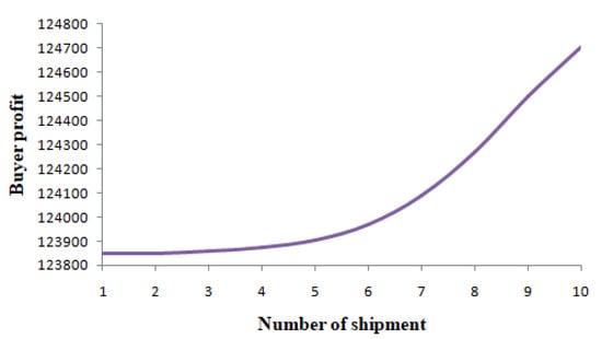
Figure 8. Impact of number of shipments on buyer’s profit.

9.2. Impact of Learning

From Table 4 and Figure 9, it is found that if the learning rate increases from 0.01 to 0.79, 0.90 to 1.30, and 2.5 to 3.90, the order quantity increases to 353 units, after which it gets more points and finally follows the learning curve concerning learning rate. The inspection time, cloudy index, and cycle time are almost fixed, while the retailer’s total profit increases when the learning rate increases. This study informs decision makers to take account of the learning effect that will help them earn more profit for their organizations. Hence, the retailer gets more information to exercise shipments.

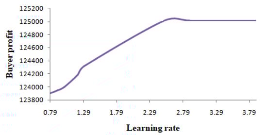
Figure 9. Impact of number of learning on buyer’s profit.

9.3. Impact of Cloudy Parameters

From Table 5, it is shown that when the cloudy parameters increase from 0.2 to 0.8, the initiative, retailer’s total profit, cycle time, cloudy index, and order lot size are almost constant. If the value of cloudy parameters increases from 0.90 to 0.99, the retailer’s total profit, cloudy index, and order lot size decrease while the cycle time increases marginally. It reflects that when a retailer wants to optimize their profit, they will have to manage the cloudy parameters.

9.4. Impact of Trade Credit

From Table 6 and Figure 10, it is shown that the effect of the trade-credit financing mechanism is accepted by the retailer on the optimal solutions. When the trade-credit period increases the retailer’s total profit, the cycle time, cloudy index, and order lot size increase while the inspection time is fixed. It indicates the retailer should always ask for long credit periods from the supplier to increase their profit.

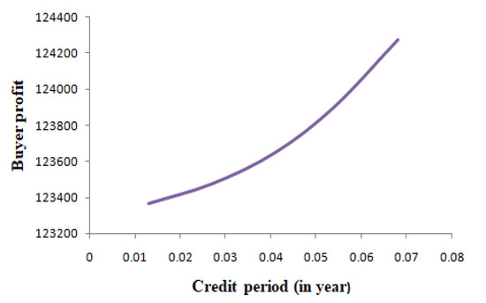
Figure 10. Impact of number of learning on buyer’s profit.

9.5. Impact of Holding Cost

From Table 7, it is found that if the holding cost increases, the order quantity, cycle time, and retailer’s total profit decrease while the cloudy index increases. It reflects that the retailer can control their cloudy index number with the help of the holding cost.

9.6. Impact of Inspection Cost

From Table 8, it is observed that if the inspection cost increases, then the order quantity, cycle time, and cloudy index remain constant, the retailer’s total profit decreases while the cloudy index increases. It reflects that retailers can manage their profit and cloudy index number with the help of the inspection cost.

9.7. Impact of Ordering Cost

From Table 9, it is observed that if the ordering cost increases, then the order quantity and cycle time increase while the retailer’s total profit decreases. The cloudy index does not change initially, but after a certain value of ordering cost, it decreases. It suggests that the retailer can manage their profit and cloudy index number with the help of the inspection cost.

9.8. Impact of Unit Purchasing Cost

From Table 10, it is observed that if the unit purchasing cost increases, then the order quantity and cycle time increase while the retailer’s total profit and cloudy index number decrease. It suggests that a retailer can manage their profit, order quantity, cycle time, and cloudy index number with the help of the unit purchasing cost. This analysis can be used when purchasing any item.

9.9. Impact of Unit Selling Price of Good Items

From Table 11, it is observed that if the unit selling price of good items increases, then the retailer’s total profit and cloudy index increase while order quantity and cycle time decrease. It suggests that a retailer can manage their profit, order quantity, cycle time, and cloudy index number in relation to unit selling price in good quantity.

9.10. Impact of Unit Selling Price of Defective Items

From Table 12, it is observed that if the unit selling price of defective items increases, then the retailer’s total profit, order quantity, and cycle time increase while the cloudy index remains constant. It means that the cloudy index number is not affected by the unit selling price of defective items. This is one piece of information for decision makers during business transactions.

10. Discussion

In this part, we will discuss the distinct cases and try to determine which case is better for this model. After getting all the values from the above three cases, we conclude that the maximum profit was given by Case 2, which is $t_n\le M\le T_n$, and it was beneficial due to the suitable credit period that was obtained from the algorithm. Other cases were not considered due to the smaller value of the credit period and were analyzed from the algorithm. Case 2 was considered because of the greater order quantity and more profit compared to Case 1, which is beneficial to the perception of the supplier and retailer. Case 3 was not considered due to a greater credit period, more risk for sellers, and less profit compared to Case 1. Case 3 also lacks coordination between the seller and buyer during the credit policy. Conclusively, pondering upon the same, we considered that Case 2 ($t_n\le M\le T_n$) is perfect for any situation. This case gave the approximate value for all parameters. When executing the algorithm, learning effects posed as cost-reduction parameters implemented by the buyer to earn a greater profit.

11. Conclusions and Future Scope

The present paper developed an EOQ model with learning and trade-credit financing under the cloudy fuzzy environment for imperfect items. The demand rate was taken as the cloudy fuzzy triangular number. This paper is different from that of De and Mahata (2019) due to the presence of learning and trade-credit financing concepts. From Table 2, it can be analyzed that the order quantity is less, but the cycle length and total profit are more in the cloudy fuzzy environment compared to the crisp and fuzzy environments. The retailer received more profit in the case of the cloudy fuzzy environment. The demand rate can be controlled by the cloudy fuzzy environment, and it is more beneficial for the retailer. Eventually, it was concluded that the results of this model showed that the number of defective units and cost reduces as learning increases and follows a form similar to a logistic curve. Slow learning resulted in order quantities that were larger than their EOQ values, and learning became faster; hence, it is recommended to order lots less frequently. When a permissible delay period is large, then the retailer is encouraged to give a big order, which eventually results in higher profit. The cloudy fuzzy model will always give the average buyer optimal profit, as shown in the present paper. The findings, together with the mathematical analysis, clearly suggest that the presence of trade credit and the learning effect had an affirmative impact on retailer ordering policy. The present work improves on more sensible positions such as the Pythagorean fuzzy set [40], supply chain management, two-level trade-credit policies, etc.

References

- Harris, F.W. How many parts to make at once. Mag. Manag. 1913, 10, 135–136. [Google Scholar] [CrossRef]
- Karlin, S.; Scarf, H. The nature and structure of inventory problems. In Studies in the Mathematical Theory of Inventory and Production; Stanford University Press: Stanford, CA, USA, 1958; pp. 16–36. [Google Scholar]
- Porteus, E.L. Optimal lot sizing, process quality improvement and setup cost reduction. Oper. Res. 1986, 34, 137–144. [Google Scholar] [CrossRef]
- Rosenblatt, M.J.; Lee, H. Improving profitability with quantity discounts under fixed demand. IIE Trans. 1985, 17, 388–395. [Google Scholar] [CrossRef]
- Rosenblatt, M.J.; Lee, H.L. Economic production cycles with imperfect production processes. IIE Tran. 1986, 18, 48–55. [Google Scholar] [CrossRef]
- Shah, N.H. A lot-size model for exponentially decaying inventory when delay in payments is permissible. Cah. Du Cent. D’études De Rech. Opérationnelle 1993, 35, 115–123. [Google Scholar]
- Shah, N.H. A probabilistic order level system when delay in payments is permissible. J. Korean Oper. Res. Manag. Sci. Soc. 1993, 18, 175–182. [Google Scholar]
- Aggarwal, S.P.; Jaggi, C.K. Ordering policies of deteriorating items under permissible delay in payments. J. Oper. Res. Soc. 1995, 46, 658–662. [Google Scholar] [CrossRef]
- Goyal, S.K. Economic order quantity under conditions of permissible delay in payments. J. Oper. Res. Soc. 1985, 36, 335–338. [Google Scholar] [CrossRef]
- Wright, T.P. Factors affecting the cost of airplanes. J. Aeronaut. Sci. 1936, 3, 122–128. [Google Scholar] [CrossRef]
- Jaber, M.Y.; Bonney, M. Optimal lot sizing under learning considerations: The bounded learning case. Appl. Math. Mod. 1996, 20, 750–755. [Google Scholar] [CrossRef]
- Jaber, M.Y.; Bonney, M. The effects of learning and forgetting on the optimal lot size quantity of intermittent production runs. Prod. Plan. Control 1998, 9, 20–27. [Google Scholar] [CrossRef]
- Jaggi, C.K.; Goel, S.K.; Mittal, M. Credit financing in economic ordering policies for defective items with allowable shortages. Appl. Math. Comput. 2013, 219, 5268–5282. [Google Scholar]
- Tiwari, S.; Daryanto, Y.; Wee, H.M. Sustainable inventory management with deteriorating and imperfect quality items considering carbon emission. J. Clean. Prod. 2018, 192, 281–292. [Google Scholar] [CrossRef]
- Jayaswal, M.K.; Sangal, I.; Mittal, M.; Malik, S. Effects of learning on retailer ordering policy for imperfect quality items with trade credit financing. Uncertain Supply Chain. Manag. 2019, 7, 49–62. [Google Scholar] [CrossRef]
- Yadav, R.; Pareek, S.; Mittal, M. Supply chain models with imperfect quality items when end demand is sensitive to price and marketing expenditure. RAIRO-Opera. Res. 2018, 52, 725–742. [Google Scholar]
- Kumar, V.; Sarkar, B.; Sharma, A.N.; Mittal, M. New product launching with pricing, free replacement, rework, and warranty policies via genetic algorithmic approach. Int. Jor. Compu. Intel. Syst. 2019, 12, 519–529. [Google Scholar] [CrossRef]
- Jaggi, C.K.; Sharma, A.; Mittal, M. A Fuzzy Inventory Model for Deteriorating Items with Initial Inspection and Allowable Shortage under the Condition of Permissible Delay in Payment. Int. J. Invent. Control Manag. 2012, 2, 167–200. [Google Scholar]
- Jaggi, C.K.; Sharma, A.; Jain, R. EOQ Model with Permissible Delay in Payments under Fuzzy Environment. In Analytical Approaches to Strategic Decision-Making: Interdisciplinary Considerations; IGI Global: Hershey, PA, USA, 2014; pp. 281–296. [Google Scholar]
- Sharma, J.P.; Kamath, H.R. Stochastic voltage stability margin in unbalance feeder with fuzzy based distributed generation placement. Int. J. Eng. Technol. 2018, 7, 53–57. [Google Scholar] [CrossRef][Green Version]
- Patro, R.; Acharya, M.; Nayak, M.M.; Patnaik, S. A fuzzy EOQ model for deteriorating items with imperfect quality using proportionate discount under learning effects. Int. J. Manag. Decis. Mak. 2018, 17, 171–198. [Google Scholar] [CrossRef]
- De, S.K.; Mahata, G.C. A cloudy fuzzy economic order quantity model for imperfect-quality items with allowable proportionate discounts. J. Ind. Eng. Int. 2019, 15, 571–583. [Google Scholar] [CrossRef]
- Hammer, K.F. An Analytical Study of Learning Curves as a Means of Labor Standards. Master’s Thesis, Cornell University, New York, NY, USA, 1954. [Google Scholar]
- Baloff, N. Startups in machine-intensive production systems. J. Ind. Eng. 1966, 17, 25–30. [Google Scholar]
- Cunningham, J.A. Using the learning curve as management tool. IEEE Spec. 1980, 17, 43–48. [Google Scholar]
- Dutton, J.R.; Thomas, A. Treating progress function as a managerial opportunity. Acad. Manag. Rev. 1984, 9, 235–247. [Google Scholar] [CrossRef]
- Argote, L.; Beckman, S.L.; Eppe, D. The persistence and transfer of learning in industrial settings. Manag. Sci. 1990, 36, 140–154. [Google Scholar] [CrossRef]
- Salameh, M.K.; Abdul-Malak, M.A.U.; Jaber, M.Y. Mathematical modelling of the effect of human learning in the finite production inventory model. Appl. Math. Model. 1993, 17, 613–615. [Google Scholar] [CrossRef]
- Salameh, M.K.; Jaber, M.Y. Economic production quantity model for items with imperfect quality. Int. J. Prod. Econ. 2000, 64, 59–64. [Google Scholar] [CrossRef]
- Jaber, M.Y.; Goyal, S.K.; Imran, M. Economic production quantity model for items with imperfect quality subject to learning effects. Int. J. Prod. Econ. 2008, 115, 143–150. [Google Scholar]
- Khan, M.; Jaber, M.Y.; Wahab, M.I.M. Economic order quantity model for items with imperfect quality with learning in inspection. Int. J. Prod. Econ. 2010, 124, 87–96. [Google Scholar] [CrossRef]
- Anzanello, M.J.; Fogliatto, F.S. Learning curve models and applications: Literature review and research directions. Int. J. Ind. Ergon. 2011, 41, 573–583. [Google Scholar] [CrossRef]
- Sarkar, B. Supply chain coordination with variable backorder, inspection and discount policy for fixed lifetime products. Math. Prob. Eng. 2016, 2016, 6318737. [Google Scholar] [CrossRef]
- Sangal, I.; Agarwal, A.; Rani, S. A fuzzy environment inventory model with partial backlogging under learning effect. Int. J. Comput. Appl. 2016, 137, 25–32. [Google Scholar] [CrossRef]
- Shin, D.; Mittal, M.; Sarkar, B. Effects of human errors and trade credit financing in two echelon supply chain models. Eur. J. Ind. Eng. 2018, 12, 263–271. [Google Scholar] [CrossRef]
- Jaggi, C.K.; Tiwari, S.; Goel, S.K. Credit financing in economic ordering policies for non-instantaneous deteriorating items with price dependent demand and two storage facilities. Ann. Oper. Res. 2007, 248, 253–280. [Google Scholar] [CrossRef]
- Nobil, A.H.; Afshar Sedigh, A.H.; Tiwari, S.; Wee, H.M. An imperfect multi-item single machine production system with shortage, rework, and scrapped considering inspection, dissimilar deficiency levels and non-zero setup times. Sci. Iran. 2019, 26, 557–570. [Google Scholar] [CrossRef]
- Nobil, A.H.; Tiwari, S.; Tajik, F. Economic production quantity model considering warm-up period in a cleaner production environment. Int. J. Prod. Res. 2018, 57, 1–14. [Google Scholar] [CrossRef]
- Jayaswal, M.K.; Sangal, I.; Mittal, M.; Tripathi, J. Fuzzy based EOQ Model with Credit Financing and Backorders under Human Learning. Int. J. Fuz. Sys. Applica. 2021, 10, 14–36. [Google Scholar] [CrossRef]
- Wang, L.; Garg, H. Algorithm for Multiple Attribute Decision-Making with Interactive Archimedean Norm Operations Under Pythagorean Fuzzy Uncertainty. Int. J. Comput. Intell. Syst. 2021, 14, 503–527. [Google Scholar] [CrossRef]
Publisher’s Note: MDPI stays neutral with regard to jurisdictional claims in published maps and institutional affiliations. |
© 2022 by the authors. Licensee MDPI, Basel, Switzerland. This article is an open access article distributed under the terms and conditions of the Creative Commons Attribution (CC BY) license (https://creativecommons.org/licenses/by/4.0/).