Mathematical Modeling and Stability Analysis of a Delayed Carbon Absorption-Emission Model Associated with China’s Adjustment of Industrial Structure

Abstract

Global warming has brought about enormous damage, therefore, some scholars have begun to conduct in-depth research on peak carbon dioxide emissions and carbon neutrality. In this paper, based on the background of China’s upgrading industrial structure and energy structure, we establish a delayed two-dimensional differential equation model associated with China’s adjustment of industrial structure. Firstly, we analyze the existence of the equilibrium for the model. We also analyze the characteristic roots of the characteristic equation at each equilibrium point for the model, then, we analyze the stability of the equilibrium point for the model according to the characteristic root, and discuss the existence of Hopf bifurcation of the system by using bifurcation theory. Secondly, we derive the normal form of Hopf bifurcation by using the multiple time scales method. Then, through the official real data, we present the range of some parameters in the model, and determine a set of parameters by reasonable analysis. The validity of the theoretical results is verified by numerical simulations. Finally, we use the real data to forecast the time of peak carbon dioxide emissions and carbon neutralization. Eventually, we put forward some suggestions based on the current situation of carbon emission and absorption in China, such as planting trees to increase the growth rate of carbon absorption, deepening industrial reform and optimizing energy structure to reduce carbon emissions.

1. Introduction

Unreasonable development has caused environmental destruction, therefore, it is the general trend to protect the environment and save energy. Global collaboration promotes the rapid development of the world; immoderate use of natural resources, however, has given rise to land degradation, deforestation and biodiversity loss, and so on. Three wastes in industrial production cause soil pollution, water pollution and air pollution, the rapid development of the global secondary industry promotes the burning of fossil fuels in large quantities, and the greenhouse gas released intensifies the greenhouse effect, causing global warming. The melting of the polar ice cap causes the sea level to rise, and some river deltas with low altitude and fertile land are submerged. At the same time, it also causes seawater to pour into the harbor, which pollutes underground water sources and aggravates the salinization of land. We can know from the notice issued by “The State of Global Climate 2020” that the global average temperature in 2020 was about 1.2 degrees Celsius higher than the pre-industrial level. In the face of natural disasters, human beings are extremely helpless. In order to slow down the trend of climate warming, the United Nations adopted the United Nations Framework Convention on Climate Change in New York on 9 May 1992. In 1997, the Kyoto Protocol of the United Nations Framework Convention on Climate Change was successfully formulated, and it provided legally binding quantitative emission reduction and emission limitation targets for developed countries. In December 2017, twenty-nine countries around the world had signed the Joint Statement on Carbon Neutrality. By September 2019, 66 countries had agreed at the United Nations Climate Action Summit that lucid waters and lush mountains are invaluable assets, and had formed the Climate Ambition Alliance. All these measures have accelerated global carbon neutrality. Britain, Sweden, France, Denmark, New Zealand, Hungary and other countries have written the goal of carbon neutrality into their laws. The EU announced that it will become the first “carbon neutral” land in the world in 2050.

China is a big carbon emitter, so it is imperative to promote peak carbon dioxide emissions and achieve carbon neutrality. According to the data of the seventh national census, China’s population has exceeded 1.4 billion, accounting for 21.5% of the world’s total population. Abundant human resources have promoted the rapid development of the secondary industry, which is dominated by manufacturing. China’s economy is developing steadily, among which the traditional manufacturing industry with high energy consumption and high carbon emission is still the main industry in China. In 2019, China’s total carbon emissions reached 10.17 billion tons, accounting for 28% of the global carbon emissions, and China’s industrial carbon emissions accounted for more than 50% of China’s total carbon emissions. Therefore, Zhang et al. [1] suggested that adjusting the industrial structure and the energy structure have become two obstacles on the road of carbon neutrality in China. Cai et al. [2] used standard methods to calculate urban carbon dioxide emissions, and established a data set of urban carbon dioxide emissions in China. As the largest developing country in the world and a responsible big country, China passed the Energy Conservation Law of the People’s Republic of China on 1 November 1997 in order to slow down the global warming trend and play a leading role among developing countries. China released the white paper “China’s Policies and Actions to Address Climate Change” in October 2008. In the meantime, China also actively participates in global climate change negotiations, strengthens communication, coordination and cooperation with other countries in the world, and makes contributions to jointly addressing the challenges of climate change and promoting global sustainable development. In September 2020, China proposed at the United Nations General Assembly that carbon dioxide emissions would peak before 2030, and that it strives to achieve carbon neutrality before 2060; In 2021, at the National People’s Congress, peak carbon dioxide emissions and carbon neutrality were written into the government work report for the first time. In the same year, the basic ideas and important measures to realize peak carbon dioxide emissions and carbon neutrality were put forward at the ninth meeting of the Central Committee of Finance and Economics. At the National People’s Congress in 2021, peak carbon dioxide emissions and carbon neutrality were written into the government work report for the first time, and China put forward the basic ideas and important measures to realize peak carbon dioxide emissions and carbon neutrality at the ninth meeting of the Central Committee of Finance and Economics in the same year.

China is a big carbon emitting country and a big energy consumption country. In 2010, the proportion of carbon emissions from coal in primary energy accounted for about 70%. For this reason, Zou et al. [3] found that the research and development of new energy will greatly promote the realization of carbon neutralization in China. New energy has become the protagonist of the third energy transformation, and will lead the future of carbon neutrality. In [4,5,6,7], the authors suggest that developing low-carbon cities, optimizing industrial structure, reducing carbon emissions from steel industry, improving carbon emission reduction technology and reducing carbon sequestration cost are important measures for China to realize peak carbon dioxide emissions and carbon neutrality ahead of schedule.

In the field of applied mathematics, there are a few researches on China’s carbon neutrality. Wang et al. [8] innovatively constructed traditional Markov probability transfer matrix and spatial Markov probability transfer matrix to explore the temporal and spatial evolution of China’s urban carbon emission performance and predict the long-term trend of carbon emission performance. Chen [9] put forward the energy supply and demand model under two related carbon emission scenarios, namely, China’s planned peak and advanced peak scenarios, and suggested that low carbon would be a basic feature of the change of energy supply and demand structure, and non-fossil energy would replace oil as the second largest energy source. Industrial structure and energy consumption structure all have significant influence on carbon dioxide emissions, especially industrial energy intensity. In [10], Guo used economic accounting methods to estimate the potential of China’s industrial carbon emission reduction from the perspective of structural emission reduction and intensity emission reduction, and further discussed the influence of industrial internal structure adjustment and energy structure optimization on industrial carbon emission peak and emission reduction potential. According to the data, during the 20 years from 2000 to 2019, the proportion of coal decreased from the original peak of 72.5% to 57.7%, and the natural gas resources increased from 2.2% to 8.4%. Li et al. [11] used the generalized Weng model to predict the regional natural gas production in China, and the prediction results show that the peak natural gas production will reach 323 billion cubic meters per year in 2036. In [12], the scholars investigate the relationship between energy consumption, economic growth and carbon dioxide emissions in Pakistan by using the annual time series data from 1965 to 2015. The estimation results of ARDL show that energy consumption and economic growth have both increased CO₂ emissions in Pakistan in the short and long term. In [13], based on China’s provincial panel data from 2004 to 2016, Liu et al. empirically analyzed the impact of ecological civilization construction on carbon emission intensity by using spatial Durbin model based on STIRPAT model. The above-mentioned scholars only consider one of carbon emission and carbon absorption, but not both. We know that only by considering both of them can we accurately and reasonably forecast the time when China will achieve peak carbon dioxide emissions and carbon neutrality. In this paper, we selected industrial structure and energy consumption structure as the influencing factors of carbon emissions.

As the processes of carbon emission and carbon absorption are time-varying processes, we can describe them by continuous differential equations. Furthermore, considering that carbon emission and carbon absorption are not only related to the current time, but also to the past time, we can use the delayed differential equation model to describe the phenomenon of the dynamic system of carbon emission and carbon absorption more truly and accurately. There is a lot of research work on delayed differential equations in many fields, such as biology, medicine, physics, and so on [14,15,16,17,18]. At present, there are few research achievements in describing carbon emission and carbon absorption model by using delayed differential equations, so the purpose of this paper is to use delayed differential equations to describe carbon emission and carbon absorption model.

The motivation of this paper is as follows. Firstly, according to the Chinese government’s goal of achieving peak carbon dioxide emissions by 2030 and carbon neutrality by 2060, we want to make some predictions and analyze whether China can achieve it under the current policy based on the carbon absorption and emission model. If there is some gap between the simulated results of the model and the ideal goal, we can put forward some policy suggestions to achieve China’s peak carbon dioxide emissions carbon neutrality goal by combining the model with the actual situation. Secondly, considering that many scholars have studied the peak carbon dioxide emissions and carbon neutrality in China from different fields, but there are few related studies on the use of delayed differential equations to describe this problem, and we try to establish a carbon absorption and emission model from the perspective of delayed differential equations to analyze the problem, and analyze this problem from different angles to see if we can get new results. Thirdly, this paper establishes a two-dimensional delayed differential equation model of carbon emission and carbon absorption, which is different from models models cited in the literature [3,4,5,6,7,8,9,10,11,12,13]. We focus on analyzing the existence and stability of equilibrium point, and the existence of system bifurcation, and studying the long-term change process of carbon emission and carbon absorption. The models cited in the literature [3,4,5,6,7,8,9,10,11,12,13] include traditional Markov probability transfer matrix and spatial Markov probability transfer matrix, energy supply and demand model, generalized Weng’s model, spatial Durbin model based on STIRPAT model, etc. The above models do not analyze the amount of carbon absorption, but the two-dimensional delayed differential equation proposed by us is not only related to carbon emission, but also to carbon absorption. We also use the knowledge of differential equations to analyze the stability of the model, focusing on the long-term stability of carbon emission and absorption, and so on.

The rest of the content is arranged as follows. In Section 2, we establish a delayed carbon absorption-emission model based on the carbon emission and carbon absorption. In Section 3, we analyze the existence and stability of equilibria and the existence of Hopf bifurcation for the model with time delay. In Section 4, we derive the normal form of the Hopf bifurcation of the above model and analyze the stability of the bifurcating periodic solutions. In Section 5, we present numerical simulations to verify the correctness of our analysis. Finally, the conclusion is drawn in Section 6.

2. Mathematical Modeling

In this paper, we consider carbon emission and carbon absorption together, and analyze the problem of carbon neutrality under China’s industrial adjustment. With the rapid development of economy and technology, we assume that carbon emissions and absorption are in a competitive relationship as a whole; this is because in the early stage of China’s economic development, the proportion of traditional industries has increased year by year. In 2007, the added value of China’s secondary industry accounted for 47.6% of the total proportion. At the same time, China’s clean energy development technology is not mature enough, the coal consumption is large and the utilization rate is low. In order to achieve economic growth, traditional high-carbon emission industries are developed, and natural resources are over-exploited, resulting in a significant increase in carbon emissions, immature carbon storage technology, and a corresponding reduction in carbon absorption. As the global climate is gradually warming, the greenhouse effect is obvious year on year, and mankind is facing serious natural disasters. China has gradually realized this great development idea of lucid waters and lush mountains are invaluable assets. In order to implement this correct development idea, our government is actively committed to reducing the coal proportion, improving the energy utilization rate, developing clean energy, shifting from the traditional high-carbon secondary industry to the green and sustainable tertiary industry, reducing carbon emissions, increasing the vegetation coverage, and striving to build a green city. When we only consider the competitive relationship between carbon emission and absorption, we can obtain the following model,

$$\left\{\begin{array}{cc}\hfill & \frac{dx\left(t\right)}{dt}=x\left(t\right)(a_1-\frac{a_1{S}_1}{N_2}y\left(t\right)),\hfill \\ \hfill & \frac{dy\left(t\right)}{dt}=y\left(t\right)(a_2-\frac{a_2{S}_2}{N_1}x\left(t\right)),\hfill \end{array}\right.$$

(1)

where $a_1$ represents the annual growth rate of carbon emission, $a_2$ represents the annual growth rate of carbon absorption, $x\left(t\right)$ represents China’s carbon emission amount at time t, $y\left(t\right)$ represents China’s carbon absorption amount at time t, $N_1$ means the maximum capacity of carbon emissions and $N_2$ means the maximum capacity of carbon absorption. $S_1$ means the competition coefficient coefficient of carbon emissions relative to carbon absorption and $S_2$ represents the competition coefficient of carbon absorption relative to carbon emission.

We think that adding carbon adsorption saturation term to the model will make the model more realistic. This is because China has a vast territory, diverse climates, wide latitudes, and a large distance from the sea. In addition, the terrain is different, and the terrain types and mountain ranges are diverse, which leads to various combinations of temperature and precipitation and different combinations of water temperatures form different types of forest vegetation. This is because the net carbon absorbed by each vegetation is the same under certain conditions every year. Furthermore, from the technical point of view, we know that the progress of carbon storage technology promotes the increase of carbon absorption, but with the relative backwardness of technology, the carbon storage technology will improve relatively slowly, resulting in the decrease of the change rate of carbon storage.

Considering that the dual wheels of optimizing industrial structure and energy structure proposed by Guo [10] could make great contributions to national emission reduction, we can use the quadratic function simulated by previous articles to express the relationship between time and carbon emissions. We can assume that the distance between annual carbon emissions and peak carbon emissions represents the speed of carbon emissions, which is reasonable, because the smaller the distance between them, the larger the carbon emissions, and the smaller the slope of the curve. In practice, it shows that as the industrial structure is gradually transferred from the secondary industry to the tertiary industry, the energy structure is also changed from coal-based primary energy to natural gas-based clean energy, and the carbon emission changes slowly.

We know that there will be a series of processes from the transformation of industrial structure and technology research and development to the application of technology in time production, which will take a certain amount of time. If the relationship between carbon emission and carbon absorption in 2022 is simulated, the carbon emission reduction technology in 2022 will increase compared with the carbon emission when the technology is mature, because the carbon emission reduction technology is just successful but immature. Therefore, we should choose the distance from the peak to the carbon emissions before 2022 as the factor that will affect the carbon emissions in 2022. Increased investment from the government in carbon emission reduction technologies and the rapid development of carbon emission reduction technologies will accelerate the transformation of industrial structure and energy structure, as well as increasing the efficiency during the period of putting into use. For this reason, we establish the following model, the descriptions of these parameters are given in Table 1, and we note that these parameters are all positive,

$$\left\{\begin{array}{cc}\hfill & \frac{dx}{dt}=x(a_1-\frac{a_1{S}_1}{N_2}y)+k(m-x(t-\tau )),\hfill \\ \hfill & \frac{dy}{dt}=y(a_2-\frac{a_2{S}_2}{N_1}x-\frac{a_2}{N_2}y).\hfill \end{array}\right.$$

(2)

Table 1. Descriptions of variables and parameters in the model (2).

Symbol	Description	Unit
x	Carbon emissions amount	${10}^2$ Mt
y	Carbon absorption amount	${10}^2$ Mt
$a_1$	Annual growth rate of carbon emissions	-
$a_2$	Annual growth rate of carbon absorption	-
k	The influence coefficient of energy structure reform on x	-
m	The peak of carbon emissions	${10}^2$ Mt
$N_1$	The maximum capacity of carbon emissions	${10}^2$ Mt
$N_2$	The maximum capacity of carbon absorptions	${10}^2$ Mt
$S_1$	The copetitive coefficient of carbon emissions relative to carbon absorptions	-
$S_2$	The copetitive coefficient of carbon absorption relative to carbon emissions	-
$\tau$	Time-delay for carbon emission reduction technology to be applied to actual production	year

For convenience, we denote that

$$c_1=\frac{a_1{S}_1}{N_2},b_2=\frac{a_2{S}_2}{N_1},c_2=\frac{a_2}{N_2},$$

then, model (2) becomes

$$\left\{\begin{array}{cc}\hfill & \frac{dx}{dt}=x(a_1-c_{1}y)+k(m-x(t-\tau )),\hfill \\ \hfill & \frac{dy}{dt}=y(a_2-b_{2}x-c_{2}y).\hfill \end{array}\right.$$

(3)

According to the initial condition of the system (3), we present a theorem about the nonnegtivity of solution of the system (3).

Theorem 1.

If $x\left(0\right)>0,y\left(0\right)>0$, the solution $x\left(t\right),y\left(t\right)$ of the system (3) with $\tau =0$ is positive.

Proof. 

First, we prove $y\left(t\right)>0$ when $t>0$ under the positive initial condition of the system (3) with $\tau =0$.

We assume that $y\left(t\right)$ is not always positive for $t>0$ and make $t_1$ be the first time that $y\left(t_1\right)=0,y^{\prime }\left(t_1\right)<0$. According to the second equation of the system (3), we can obtain $y^{\prime }\left(t_1\right)=0$. The two conclusions we obtain are contradictory. Therefore, under the positive initial condition, the solution $y\left(t\right)$ of the system (3) is positive for $t>0$. Then, we prove $x\left(t\right)>0$ when $t>0$ under the positive initial condition of the system (3) with $\tau =0$. We assume that $x\left(t\right)$ is not always positive for $t>0$ and make $t_2$ be the first time that $x\left(t_2\right)=0,x^{\prime }\left(t_2\right)<0$. According to the first equation of the system (3), we can obtain $x^{\prime }\left(t_2\right)=km>0$. The two conclusions we reach are contradictory. Therefore, under the positive initial condition, the solution $x\left(t\right)$ of the system (3) with $\tau =0$ is also positive for $t>0$.  □

Remark 1.

We prove if $x\left(0\right)>0,y\left(0\right)>0$, the solution $x\left(t\right),y\left(t\right)$ of the system (3) with $\tau =0$ is positive. It is also not easy for us to prove the solution of the system (3) is positive when $\tau >0$. However, according to the numerical simulation of a group of real parameters, we find that the solution of the system (3) is always positive, which is not contradictory to the positivity of the solution of the system (3).

Next, we will consider the dynamics phenomena of the system (3).

3. Stability Analysis of Equilibrium and Existence of Hopf Bifurcation

In this section, we will discuss the stability of equilibria and the existence of Hopf bifurcation for system (3).

3.1. Existence of Equilibrium Point

When the parameters of system (3) meet the following assumptions

$$\left(H_1\right)k-a_1>0,$$

(4)

system (3) has a boundary equilibrium $E_1=(x^{\left(1\right)},0)$, where

$$x^{\left(1\right)}=\frac{km}{k-a_1}.$$

When the parameters of system (3) meet the following assumptions

$$\left(H_2\right)\left\{\begin{array}{cc}\hfill & \sqrt{{(c_1{a}_2+(k-a_1)c_2)}^2-4c_1{c}_2{b}_{2}km}>0,\hfill \\ \hfill & c_1{a}_2+(k-a_1)c_2+\sqrt{{(c_1{a}_2+(k-a_1)c_2)}^2-4c_1{c}_2{b}_{2}km}>0,\hfill \\ \hfill & c_1{a}_2-(k-a_1)c_2-\sqrt{{(c_1{a}_2+(k-a_1)c_2)}^2-4c_1{c}_2{b}_{2}km}>0,\hfill \end{array}\right.$$

(5)

system (3) has a positive equilibrium $E_2=(x^{\left(2\right)},y^{\left(2\right)}),$ where

$$x^{\left(2\right)}=\frac{c_1{a}_2+(k-a_1)c_2+\sqrt{{(c_1{a}_2+(k-a_1)c_2)}^2-4c_1{c}_2{b}_{2}km}}{2c_1{b}_2},$$

$$y^{\left(2\right)}=\frac{c_1{a}_2-(k-a_1)c_2-\sqrt{{(c_1{a}_2+(k-a_1)c_2)}^2-4c_1{c}_2{b}_{2}km}}{2c_1{c}_2}.$$

When the parameters of system (3) meet the following assumptions

$$\left(H_3\right)\left\{\begin{array}{cc}\hfill & \sqrt{{(c_1{a}_2+(k-a_1)c_2)}^2-4c_1{c}_2{b}_{2}km}>0,\hfill \\ \hfill & c_1{a}_2+(k-a_1)c_2-\sqrt{{(c_1{a}_2+(k-a_1)c_2)}^2-4c_1{c}_2{b}_{2}km}>0,\hfill \\ \hfill & c_1{a}_2-(k-a_1)c_2+\sqrt{{(c_1{a}_2+(k-a_1)c_2)}^2-4c_1{c}_2{b}_{2}km}>0,\hfill \end{array}\right.$$

(6)

system (3) has a positive equilibrium $E_3=(x^{\left(3\right)},y^{\left(3\right)}),$ where

$$x^{\left(3\right)}=\frac{c_1{a}_2+(k-a_1)c_2-\sqrt{{(c_1{a}_2+(k-a_1)c_2)}^2-4c_1{c}_2{b}_{2}km}}{2c_1{b}_2},$$

$$y^{\left(3\right)}=\frac{c_1{a}_2-(k-a_1)c_2+\sqrt{{(c_1{a}_2+(k-a_1)c_2)}^2-4c_1{c}_2{b}_{2}km}}{2c_1{c}_2}.$$

3.2. Stability and Existence of Hopf Bifurcation for $E_1=(x^{\left(1\right)},0)$

When $\left(H_1\right)$ holds, system (3) has equilibrium $E_1$, similar to the calculation method in [19,20,21,22], we calculate the stability of the equilibrium $E_1$ and the existence of Hopf bifurcation. The characteristic equation of system (3), evaluated at $E_1$, is given as follows:

$$\lambda (\lambda -a_1+e^{-\lambda \tau }k)=0.$$

(7)

Note that $\lambda =0$ is always the root of the Equation (7). Next, we only need to consider the following equation,

$$\lambda -a_1+e^{-\lambda \tau }k=0.$$

(8)

When $\tau =0$, Equation (6) becomes

$$\lambda +k-a_1=0,$$

(9)

it leads to ${\lambda }_1=-(k-a_1)<0$, due to $\left(H_1\right)$ holds.

When $\tau >0$, we try to discuss the existence of Hopf bifurcation. We assume that $\lambda =i\omega (\omega >0)$ is a pure imaginary root of Equation (6). Substituting it into Equation (6) and separating the real and imaginary parts, we obtain:

$$\left\{\begin{array}{cc}\hfill & ksin\left(\omega \tau \right)=\omega ,\hfill \\ \hfill & kcos\left(\omega \tau \right)=a_1.\hfill \end{array}\right.$$

(10)

Equation (10) derives the following results,

$$Q_1\triangleq sin\left({\omega }_1{\tau }_1\right)=\frac{{\omega }_1}{k},R_1\triangleq cos\left({\omega }_1{\tau }_1\right)=\frac{a_1}{k}.$$

(11)

Adding the square of the two equations, we obtain

$${\omega }_1^2-a_1^2+k^2=0,$$

(12)

then it gives ${\omega }_1=\sqrt{k^2-a_1^2}$, which makes sense due to the assumptions $\left(H_1\right)$. We obtain the expression of ${\tau }_1^{\left(j\right)}$ as follows:

$${\tau }_1^{\left(j\right)}=\left\{\begin{array}{cc}\hfill & \frac{arccos\left(R_1\right)+2j\pi }{{\omega }_1},Q_1>0,\hfill \\ \hfill & \frac{-arccos\left(R_1\right)+2(j+1)\pi }{{\omega }_1},Q_1<0,j=0,1,2,3,4,\cdots .\hfill \end{array}\right.$$

(13)

Let $\lambda =\lambda \left(\tau \right)$ be the root of Equation (6), satisfying $\lambda \left({\tau }_1^{\left(j\right)}\right)=\mathrm{i}{\omega }_1$. Differentiating both sides of (6) with respective to $\tau$ gives that

$$\mathrm{Re}{\left(\frac{d\lambda }{d\tau }\right)}^{-1}{|}_{\tau ={\tau }_1^{\left(j\right)}}=\frac{k^2-a_1^2}{k{\omega }_1^2}>0.$$

(14)

Theorem 2.

When the parameters of system (3) meet the assumptions $\left(H_1\right)$, for any of $\tau ⩾0$, characteristic Equation (7) has a zero root. When $\tau ={\tau }_1^{\left(j\right)}$, characteristic Equation (7) has a zero root and a pair of pure imaginary roots, and when $\tau \in [0,{\tau }_1^{\left(0\right)})$, Equation (7) has a zero root, and other roots have negative real parts, when $\tau >{\tau }_1^{\left(0\right)}$, the equilibrium $E_1$ of system (3) is unstable.

3.3. Stability and Existence of Hopf Bifurcation for $E_{2,3}$

Next, we analyze the stability of system (3) for $E_i=(x^{\left(i\right)},y^{\left(i\right)})(i=2,3),$ and the characteristic equation of system (3), evaluated at $E_i$, is given by

$${\lambda }^2+(-a_1+c_1{y}^{\left(i\right)}+c_2{y}^{\left(i\right)})\lambda +c_2{y}^{\left(i\right)}(-a_1+c_1{y}^{\left(i\right)})-c_1{b}_2{x}^{\left(i\right)}{y}^{\left(i\right)}+(k\lambda +k{c}_2{y}^{\left(i\right)})e^{-\lambda \tau }=0.$$

(15)

When $\tau =0$, Equation (15) becomes

$${\lambda }^2+T_2^{\left(i\right)}\lambda +D_2^{\left(i\right)}=0,$$

(16)

where

$$T_2^{\left(i\right)}=(k-a_1+c_1{y}^{\left(i\right)}+c_2{y}^{\left(i\right)}),D_2^{\left(i\right)}=c_2{y}^{\left(i\right)}(k-a_1+c_1{y}^{\left(i\right)})-c_1{b}_2{x}^{\left(i\right)}{y}^{\left(i\right)}.$$

where $(x^{\left(i\right)},y^{\left(i\right)})=(x^{\left(2\right)},y^{\left(2\right)})$, the parameters of system (3) meet the assumptions $\left(H_2\right)$, we can prove that

$$T_2^{\left(2\right)}>0,D_2^{\left(2\right)}=-y^{\left(2\right)}\sqrt{{(c_1{a}_2+(k-a_1)c_2)}^2-4c_1{c}_2{b}_{2}km}<0,$$

(17)

thus, $E_2$ is unstable when $\tau =0$.

When $(x^{\left(i\right)},y^{\left(i\right)})=(x^{\left(3\right)},y^{\left(3\right)})$ and the parameters of system (3) satisfy the assumptions $\left(H_3\right)$, we can prove that

$$T_2^{\left(3\right)}>0,D_2^{\left(3\right)}=y^{\left(3\right)}\sqrt{{(c_1{a}_2+(k-a_1)c_2)}^2-4c_1{c}_2{b}_{2}km}>0,$$

(18)

thus, $E_3$ is locally asymptotically stable when $\tau =0$. When $\tau >0$, we try to discuss the existence of Hopf bifurcation. We assume that $\lambda =i\omega (\omega >0)$ is a pure imaginary root of Equation (15). Substituting it into Equation (15) and separating the real and imaginary parts, we obtain:

$$\left\{\begin{array}{cc}\hfill & {\omega }^2+c_2{y}^{\left(i\right)}(a_1-c_1{y}^{\left(i\right)})+c_1{b}_2{x}^{\left(i\right)}{y}^{\left(i\right)}=k\omega sin\left(\omega \tau \right)+k{c}_2{y}^{\left(i\right)}cos\left(\omega \tau \right),\hfill \\ \hfill & \omega (a_1-c_1{y}^{\left(i\right)}-c_2{y}^{\left(i\right)})=k\omega cos\left(\omega \tau \right)-k{c}_2{y}^{\left(i\right)}sin\left(\omega \tau \right),\hfill \end{array}\right.$$

(19)

Equation (19) derives the following results,

$$\begin{array}{cc}\hfill & Q_2^{\left(i\right)}\triangleq sin\left(\omega \tau \right)=\frac{k\omega ({\omega }^2+c_2{y}^{\left(i\right)}(a_1-c_1{y}^{\left(i\right)})+c_1{b}_2{x}^{\left(i\right)}{y}^{\left(i\right)})-k{c}_2{y}^{\left(i\right)}\omega (a_1-c_1{y}^{\left(i\right)}-c_2{y}^{\left(i\right)})}{k^2{\omega }^2+k^2{c}_2^2{y}^{\left(i\right)2}},\hfill \\ \hfill & R_2^{\left(i\right)}\triangleq cos\left(\omega \tau \right)=\hfill \\ & \frac{k{\omega }^2(a_1-c_1{y}^{\left(i\right)})+c_1{b}_2{x}^{\left(i\right)}{y}^{\left(i\right)})+k{c}_2{y}^{\left(i\right)}({\omega }^2+c_2{y}^{\left(i\right)}(a_1-c_1{y}^{\left(i\right)})+c_1{b}_2{x}^{\left(i\right)}{y}^{\left(i\right)})}{k^2{\omega }^2+k^2{c}_2^2{y}^{\left(i\right)2}}.\hfill \end{array}$$

(20)

Adding the square of the two equations, we obtain

$${\omega }^4+T_3^{\left(i\right)}{\omega }^2+D_3^{\left(i\right)}=0,$$

(21)

where

$$\begin{array}{cc}\hfill & T_3^{\left(i\right)}=2c_2{y}^{\left(i\right)}(a_1-c_1{y}^{\left(i\right)})+2c_1{b}_2{x}^{\left(i\right)}{y}^{\left(i\right)}+{(a_1-c_1{y}^{\left(i\right)}-c_2{y}^{\left(i\right)})}^2-k^2,\hfill \\ \hfill & D_3^{\left(i\right)}=2c_1{c}_2{b}_2{x}^{\left(i\right)}{y}^{\left(i\right)2}(a_1-c_1{y}^{\left(i\right)})+{\left(c_2{y}^{\left(i\right)}(a_1-c_1{y}^{\left(i\right)})\right)}^2+{\left(c_1{b}_2{x}^{\left(i\right)}{y}^{\left(i\right)}\right)}^2-{\left(k{c}_2{y}^{\left(i\right)}\right)}^2.\hfill \end{array}$$

For convenience, we let ${\omega }^2=z$, Equation (21) becomes

$$h\left(z\right)=z^2+T_3^{\left(i\right)}z+D_3^{\left(i\right)}=0.$$

(22)

When the parameters of system (3) meet the following assumptions—$D_3^{\left(i\right)}<0$, Equation (22) has one positive root $z_2$; If $T_3^{\left(i\right)}>0,D_3^{\left(i\right)}>0$ hold, Equation (22) has no positive root; If $T_3^{\left(i\right)}<0,D_3^{\left(i\right)}>0$ hold, Equation (22) has two positive roots $z_3,z_4$. We hypothesize that Equation (22) has positive roots $z_n(n=2,3,4)$, then ${\omega }_n=\sqrt{z_n}(n=2,3,4)$. From (20), we can solve the critical value of time delay,

$${\tau }_n^{\left(j\right)}=\left\{\begin{array}{cc}\hfill & \frac{arcsin\left(Q_2^{\left(i\right)}\right)+2j\pi }{{\omega }_n},R_2>0,\hfill \\ \hfill & \frac{-arcsin\left(Q_2^{\left(i\right)}\right)+2(j+1)\pi }{{\omega }_n},R_2<0,n=2,3,4,j=0,1,2,\cdots .\hfill \end{array}\right.$$

(23)

Let $\lambda =\lambda \left(\tau \right)$ be the root of (15), satisfying $\lambda \left({\tau }_n^{\left(j\right)}\right)=i{\omega }_n(n=2,3,4).$ Differentiating both sides of Equation (15) with respective to $\tau$ gives that:

$$\begin{array}{cc}\hfill \mathrm{Re}{\left(\frac{d\lambda }{d\tau }\right)}^{-1}{|}_{\tau ={\tau }_n^{\left(j\right)}}& =\frac{2{\omega }_n^2+2c_2{y}^{\left(i\right)}(a_1-c_1{y}^{\left(i\right)})+2c_1{b}_2{x}^{\left(i\right)}{y}^{\left(i\right)}+{(a_1-c_1{y}^{\left(i\right)}-c_2{y}^{\left(i\right)})}^2-k^2}{k^2{\omega }_n^2+k^2{c}_2^2{y}^{\left(i\right)2}}\hfill \\ \hfill & =h^{\prime }\left(z_n\right)\ne 0.\hfill \end{array}$$

(24)

Theorem 3.

Considering the stability of $E_2$ and $E_3$ for system (3), we come to the following conclusions:

• (1) When $\left(H_2\right)$ holds, the equilibrium $E_2$ is unstable for any $\tau ⩾0$;
• (2) When $\left(H_3\right)$ holds, we discuss the stability of equilibrium $E_3$ of system (3) below.

(a) When $T_3^{\left(3\right)}>0,D_3^{\left(3\right)}>0$ hold, Equation (22) has no positive root, the equilibrium $E_3$ is locally asymptotically stable for any $\tau ⩾0$;

(b) If $D_3^{\left(3\right)}<0$ holds, Equation (22) has one positive roots $z_2$, then when $\tau \in [0,{\tau }_2^{\left(0\right)})$, the equilibrium $E_3$ is locally asymptotically stable, and unstable when $\tau >{\tau }_2^{\left(0\right)}$;

(c) If $T_3^{\left(3\right)}<0,D_3^{\left(3\right)}>0$ hold, system (3) undergoes a Hopf bifurcation at the trivial equilibrium $E_3$ when $\tau ={\tau }_n^{\left(j\right)}(n=3,4;j=0,1,2,\cdots )$. Then, $\exists m\in N$ makes $0<{\tau }_4^{\left(0\right)}<{\tau }_3^{\left(0\right)}<{\tau }_4^{\left(1\right)}<{\tau }_4^{\left(1\right)}<\cdots <{\tau }_3^{(m-1)}<{\tau }_4^{\left(m\right)}<{\tau }_4^{(m+1)}$. When $\tau \in [0,{\tau }_4^{\left(0\right)})\cup \bigcup _{l=1}^m({\tau }_3^{(l-1)},{\tau }_4^{\left(l\right)})$, the equilibrium $E_3$ of the system (3) is locally asymptotically stable, and when $\tau \in \bigcup _{l=0}^{m-1}({\tau }_4^{\left(l\right)},{\tau }_3^{\left(l\right)})\cup ({\tau }_4^{\left(m\right)},+\infty )$, the equilibrium $E_3$ is unstable.

Proof. 

(1)

When $\left(H_2\right)$ and $\tau =0$ hold, we can prove $T_2^{\left(2\right)}>0,D_2^{\left(2\right)}<0$, that is Equation (16) has a positive root, so equilibrium $E_2$ of system (3) with $\tau =0$ is unstable;

(2)

When $T_3^{\left(3\right)}>0,D_3^{\left(3\right)}>0$ hold, we can prove $T_2^{\left(3\right)}>0,D_2^{\left(3\right)}>0$, that is, Equation (16) has two negative roots, so equilibrium $E_3$ of system (3) with $\tau =0$ is locally asymptotically stable:

(a)

When $T_3^{\left(3\right)}>0,D_3^{\left(3\right)}>0$ hold, Equation (22) has no positive root, the equilibrium $E_3$ is locally asymptotically stable for any $\tau ⩾0$;

(b)

When $D_3^{\left(3\right)}<0$ holds, Equation (22) has one positive root $z_2$, and $Sign\left(\mathrm{Re}{\left(\frac{d\lambda }{d\tau }\right)}_{\tau ={\tau }_2^{\left(j\right)}}^{-1}\right)=Sign\left(h^{\prime }\left(z_2\right)\right)>0$, and thus, all the roots of Equation (22) have negative real parts for $\tau \in [0,{\tau }_2^{\left(0\right)})$, and Equation (22) has at least one pair of roots with positive real part when $\tau >{\tau }_2^{\left(0\right)}$;

(c)

If $T_3^{\left(3\right)}<0,D_3^{\left(3\right)}>0$ hold, $h\left(z\right)=0$ has two positive roots $z_3$ and $z_4$, and $Sign\left(\mathrm{Re}{\left(\frac{d\lambda }{d\tau }\right)}_{\tau ={\tau }_3^{\left(j\right)}}^{-1}\right)=Sign\left(h^{\prime }\left(z_3\right)\right)<0$ and $Sign\left(\mathrm{Re}{\left(\frac{d\lambda }{d\tau }\right)}_{\tau ={\tau }_4^{\left(j\right)}}^{-1}\right)$ $=Sign\left(h^{\prime }\left(z_4\right)\right)>0$, thus, there exists $m\in N$, such that all the roots of Equation (15) have negative real parts when $\tau \in [0,{\tau }_4^{\left(0\right)})\cup \bigcup _{l=1}^m({\tau }_3^{(l-1)},{\tau }_4^{\left(l\right)})$, and Equation (15) has at least one root with a positive real part when $\tau \in \bigcup _{l=0}^{m-1}({\tau }_4^{\left(l\right)},{\tau }_3^{\left(l\right)})\cup ({\tau }_4^{\left(m\right)},+\infty )$, and the conclusion is immediate.

 □

4. Normal Form of Hopf Bifurcation

In Section 3, we have shown that the equilibrium $E_2=(x^{\left(2\right)},y^{\left(2\right)})$ is unstable when $\tau =0$, and the equilibrium $E_3=(x^{\left(3\right)},y^{\left(3\right)})$ is locally asymptotically stable when $\tau =0$. To reflect the actual situation, we focus on the delay from technological innovation to practical production. Therefore, we consider the time-delay $\tau$ as a bifurcation parameter and denote the critical value $\tau ={\tau }_c={\tau }_n^{\left(j\right)}$, where ${\tau }_n^{\left(j\right)}$ is given in (23). When $\tau ={\tau }_n^{\left(j\right)}$, characteristic Equation (21) has a pair of pure imaginary roots $\lambda =\pm i\omega$. Therefore, system (3) undergoes a Hopf bifurcation at equilibrium $E_3$. In this section, we derive the normal form of Hopf bifurcation for the system (3) by using the multiple time scales method given in [23,24].

In order to normalize the delay, we first re-scale the time t by using $t\mapsto t/\tau$, then translate the equilibrium $E_3=(x^{\left(3\right)},y^{\left(3\right)})$ to the origin, that is,

$$\left\{\begin{array}{cc}\hfill & \tilde{x}=x-x^{\left(3\right)},\hfill \\ \hfill & \tilde{y}=y-y^{\left(3\right)},\hfill \end{array}\right.$$

For convenience, we still use x and y to represent $\tilde{x}$ and $\tilde{y}$ respectively, so Equation (3) is transformed into:

$$\left\{\begin{array}{cc}\hfill & \frac{dx}{dt}=\tau (a_{1}x-c_1{x}^{\left(3\right)}y-c_{1}xy-c_1{y}^{\left(3\right)}x-kx(t-1)),\hfill \\ \hfill & \frac{dy}{dt}=-\tau (y+y^{\left(3\right)})(b_{2}x+c_{2}y).\hfill \end{array}\right.$$

(25)

Equation (25) can also be written as:

$$\dot{Z}\left(t\right)=\tau N_{1}Z\left(t\right)+\tau N_{2}Z(t-1)+\tau F(Z\left(t\right),Z(t-1)),$$

(26)

where

$$Z\left(t\right)={(x\left(t\right),y\left(t\right))}^T,Z(t-1)={(x(t-1),y(t-1))}^T,F(Z\left(t\right),Z(t-1))={(x(t-1),y(t-1))}^T,$$

and

$$N_1=\left(\begin{array}{cc}{a}_1-c_1{y}^{\left(3\right)}& -c_1{x}^{\left(3\right)}\\ -b_2{y}^{\left(3\right)}& -c_2{y}^{\left(3\right)}\end{array}\right),N_2=\left(\begin{array}{cc}-k& 0\\ 0& 0\end{array}\right).$$

We let h be eigenvector corresponding to eigenvalue $\lambda =i\omega \tau$ of Equation (26), and $h^{*}$ be the eigenvector corresponding to eigenvalue $\lambda =-i\omega \tau$ of adjoint matrix of Equation (26), satisfying

$$<h^{*},h>={\overline{h^{*}}}^{T}h=1.$$

(27)

By calculating, we have

$$h={(1,-\frac{b_2{y}^{\left(3\right)}}{i\omega +c_2{y}^{\left(3\right)}})}^T,h^{*}=d{(\frac{i\omega -c_2{y}^{\left(3\right)}}{c_1{x}^{\left(3\right)}},1)}^T,d=\frac{c_1{x}^{\left(3\right)}}{c_1{x}^{\left(3\right)}+b_2{y}^{\left(3\right)}}.$$

(28)

We treat the delay $\tau$ as the bifurcation parameter, let $\tau ={\tau }_c+\epsilon \mu$, where ${\tau }_c={\tau }_n^{\left(j\right)}$ $(j=0,1,2,\cdots )$ is the Hopf bifurcation critical value, $\mu$ is perturbation parameter, $\epsilon$ is dimensionless scale parameter. Suppose system (26) undergoes a Hopf bifurcation from the trivial equilibrium at the critical point $\tau ={\tau }_c$, and then, by the MTS method, the solution of (26) is assumed as follows:

$$Z\left(t\right)=Z(T_0,T_1,T_2,\cdots )=\sum _{k=1}^{+\infty }{\epsilon }^k{Z}_k(T_0,T_1,T_2,\cdots ),$$

(29)

where

$$\begin{array}{cc}\hfill & Z(T_0,T_1,T_2,\cdots )={(x(T_0,T_1,T_2,\cdots ),y(T_0,T_1,T_2,\cdots ))}^T,\hfill \\ \hfill & Z_k(T_0,T_1,T_2,\cdots )={(x_k(T_0,T_1,T_2,\cdots ),y_k(T_0,T_1,T_2,\cdots ))}^T,\hfill \end{array}$$

and the derivative with regard to t is transformed into

$$\frac{d}{dt}=\frac{\partial }{\partial T_0}+\epsilon \frac{\partial }{\partial T_1}+{\epsilon }^2\frac{\partial }{\partial T_2}+\cdots =D_0+\epsilon D_1+{\epsilon }^2{D}_2+\cdots ,$$

(30)

where $D_i$ is differential operator, and

$$D_i=\frac{\partial }{\partial T_i}(i=0,1,2,3,\cdots ).$$

From (26), we have

$$\dot{Z}\left(t\right)=\epsilon D_0{Z}_1+{\epsilon }^2{D}_1{Z}_1+{\epsilon }^3{D}_2{Z}_1+{\epsilon }^2{D}_0{Z}_2+{\epsilon }^3{D}_1{Z}_2+{\epsilon }^3{D}_0{Z}_3+\cdots .$$

(31)

We expand $x(T_0-1,\epsilon (T_0-1),{\epsilon }^2(T_0-1),\cdots )$ at $x(T_0-1,T_1,T_2,\cdots )$ by the Taylor expansion, that is,

$$x(t-1)=\epsilon x_{1,{\tau }_c}+{\epsilon }^2{x}_{2,{\tau }_c}+{\epsilon }^3{x}_{3,{\tau }_c}-{\epsilon }^2{D}_1{x}_{1,{\tau }_c}-{\epsilon }^3{D}_2{x}_{1,{\tau }_c}-{\epsilon }^3{D}_1{x}_{2,{\tau }_c}+\cdots ,$$

(32)

where $x_{j,{\tau }_c}=x_j(T_0-1,T_1,T_2,\cdots ),j=1,2,3\cdots .$

We substitute Formulas (29)–(32) into Equation (26), then comparing the coefficients of $\epsilon ,{\epsilon }^2$ and ${\epsilon }^3$ on both sides of the equation, respectively. Then, we obtain the following expressions, respectively,

$$\begin{array}{cc}\hfill & D_0{x}_1-{\tau }_c(a_1{x}_1-c_1{x}^{\left(3\right)}{y}_1-c_1{x}_1{y}^{\left(3\right)}-k{x}_{1,{\tau }_c})=0,\hfill \\ \hfill & D_0{y}_1+{\tau }_c{y}^{\left(3\right)}(b_2{x}_1+c_2{y}_1)=0.\hfill \end{array}$$

(33)

$$\begin{array}{cc}\hfill & D_0{x}_2-{\tau }_c(a_1{x}_2-c_1{x}^{\left(3\right)}{y}_2-c_1{x}_2{y}^{\left(3\right)}-k{x}_{2,{\tau }_c})\hfill \\ \hfill =& \mu (a_1{x}_1-c_1{x}^{\left(3\right)}{y}_1-c_1{x}_1{y}^{\left(3\right)}-k{x}_{1,{\tau }_c})-{\tau }_c(c_1{x}_1{y}_1-k{D}_1{x}_{1,{\tau }_c})-D_1{x}_1,\hfill \\ \hfill & D_0{y}_2+{\tau }_c{y}^{\left(3\right)}(b_2{x}_2+c_2{y}_2)\hfill \\ \hfill =& -(\mu y^{\left(3\right)}+{\tau }_c{y}_1)(b_2{x}_1+c_2{y}_1)-D_1{y}_1.\hfill \end{array}$$

(34)

$$\begin{array}{cc}\hfill & D_0{x}_3-{\tau }_c(a_1{x}_3-c_1{x}^{\left(3\right)}{y}_3-c_1{x}_3{y}^{\left(3\right)}-k{x}_{3,{\tau }_c})\hfill \\ \hfill =& \mu (a_1{x}_2-c_1{x}_2{y}_1-c_1{x}^{\left(3\right)}{y}_2-c_1{x}_2{y}^{\left(3\right)}+k{x}_{2,{\tau }_c}+k{D}_1{x}_{1,{\tau }_c})-{\tau }_c(c_1{x}_2{y}_1+c_1{x}_1{y}_2-\hfill \\ & k{D}_2{x}_{1,{\tau }_c}-k{D}_1{x}_{2,{\tau }_c})-D_1{x}_2-D_2{x}_1,\hfill \\ \hfill & D_0{y}_3+{\tau }_c{y}^{\left(3\right)}(b_2{x}_3+c_2{y}_3)\hfill \\ \hfill =& -{\tau }_c(y_2(b_{2}x-1+c_2{y}_1)+y_1(b_2{x}_2+c_2{y}_2))-\mu (y_1(b_2{x}_1+c_2{y}_1)+y^{\left(3\right)}(b_2{x}_2+c_2{y}_2))\hfill \\ & -D_1{y}_2-D_2{y}_1.\hfill \end{array}$$

(35)

Equation (33) has the solution with following form,

$$Z_1=Gh{e}^{i\omega {\tau }_c{T}_0}+\overline{G}\overline{h}{e}^{-i\omega {\tau }_c{T}_0},$$

(36)

where h is given by (28). Equation (34) is a linear non-homogeneous equation, and the non-homogeneous equation has a solution if and only if a solvability condition is satisfied. That is, the right-hand side of (34) should be orthogonal to every solution of the adjoint homogeneous problem. Thus, we solve (36) into the right part of equation (34), and the coefficient vector of $e^{i\omega {\tau }_c{T}_0}$ is noted as $m_1$, by $<h^{*},m_1>=0,$ so we can solve $\frac{\partial G}{\partial T_1}$, namely,

$$\frac{\partial G}{\partial T_1}=M\mu G,$$

(37)

where

$$\begin{array}{cc}\hfill & M=\frac{c_1{x}^{\left(3\right)}(y^{\left(3\right)}{b}_2+y^{\left(3\right)}{c}_2{h}_2)-(c_2{y}^{\left(3\right)}+i\omega )(-a_1+c_1{x}^{\left(3\right)}{h}_2+c_1{y}^{\left(3\right)}+k{e}^{-i\omega {\tau }_c})}{(c_2{y}^{\left(3\right)}+i\omega )(-{\tau }_{c}k{e}^{-i\omega {\tau }_c}+1)-c_1{x}^{\left(3\right)}{h}_2},\hfill \\ \hfill & h_2=-\frac{b_2{y}^{\left(3\right)}}{i\omega +c_2{y}^{\left(3\right)}},\hfill \end{array}$$

with

$$\begin{array}{cc}\hfill & x^{\left(3\right)}=\frac{c_1{a}_2+(k-a_1)c_2-\sqrt{{(c_1{a}_2+(k-a_1)c_2)}^2-4c_1{c}_2{b}_{2}km}}{2c_1{b}_2},\hfill \\ \hfill & y^{\left(3\right)}=\frac{c_1{a}_2-(k-a_1)c_2+\sqrt{{(c_1{a}_2+(k-a_1)c_2)}^2-4c_1{c}_2{b}_{2}km}}{2c_1{c}_2}.\hfill \end{array}$$

We solve Equation (34), as $\mu$ is a small disturbance coefficient, and we only consider the influence of $\mu$ on low-order terms, thus, we obtain its solutions with following form:

$$\begin{array}{cc}\hfill & x_2=g_1{e}^{2i\omega {\tau }_c{T}_0}+c.c.+l_1,\hfill \\ \hfill & y_2=g_2{e}^{2i\omega {\tau }_c{T}_0}+c.c.+l_2,\hfill \end{array}$$

(38)

where $c.c.$ stands for the complex conjugate of the preceding terms, then, we substitute solutions (38) into (34), and we obtain

$$\begin{array}{cc}\hfill & g_1=K_{1}S{G}^2,l_1=P_{1}RG\overline{G},\hfill \\ \hfill & g_2=K_{2}S{G}^2,l_2=P_{2}RG\overline{G},\hfill \end{array}$$

(39)

with

$$\begin{array}{cc}\hfill & K_1=(2i\omega +c_2{y}^{\left(3\right)})(-c_1{h}_2)+c_1{x}^{\left(3\right)}(c_2{h}_2^2+b_2{h}_2),\hfill \\ \hfill & K_2=(2i\omega +c_1{y}^{\left(3\right)}-a_1+k{e}^{-2i\omega {\tau }_c})(-c_2{h}_2^2-b_2{h}_2)+c_1{b}_2{y}^{\left(3\right)}{h}_2,\hfill \\ \hfill & S={((2i\omega +c_2{y}^{\left(3\right)})(2i\omega +c_1{y}^{\left(3\right)}-a_1+k{e}^{-2i\omega {\tau }_c})-c_1{b}_2{y}^{\left(3\right)}{x}^{\left(3\right)})}^{-1},\hfill \\ \hfill & P_1=-c_1{x}^{\left(3\right)}(b_2(\overline{h_2}+h_2)+2c_2{h}_2\overline{h_2})+c_2{c}_1{y}^{\left(3\right)}(\overline{h_2}+h_2),\hfill \\ \hfill & P_2=-c_1{b}_2{y}^{\left(3\right)}(\overline{h_2}+h_2)+(c_1{y}^{\left(3\right)}+k-a_1)(b_2(\overline{h_2}+h_2)+2c_2{h}_2\overline{h_2}),\hfill \\ \hfill & R={(-c_2{y}^{\left(3\right)}(k-a_1+c_1{y}^{\left(3\right)})+c_1{b}_2{x}^{\left(3\right)}{y}^{\left(3\right)})}^{-1},h_2=-\frac{b_2{y}^{\left(3\right)}}{i\omega +c_2{y}^{\left(3\right)}}.\hfill \end{array}$$

(40)

Next, substituting solution (36) and (38) into (35), and with the coefficient vector of $e^{i\omega {\tau }_c{T}_0}$ noted as $m_2$, by solvability condition, we have $<h^{*},m_2>=0.$ Note that $\mu$ is a disturbance parameter, and ${\mu }^2$ has little influence for small unfolding parameter, thus, we can ignore the ${\mu }^{2}G$ term, then $\frac{\partial G}{\partial T_2}$, can be solved to yield

$$\frac{\partial G}{\partial T_2}=H{G}^2\overline{G},$$

(41)

where

$$\begin{array}{cc}\hfill H=& \frac{(i\omega +c_2{y}^{\left(3\right)})(-{\tau }_c{c}_1)(K_{1}S\overline{h_2}+K_{2}S+P_{1}R{h}_2+P_{2}R)}{(i\omega +c_2{y}^{\left(3\right)})(k{\tau }_c{e}^{-i\omega {\tau }_c}-1)+c_1{x}^{\left(3\right)}{h}_2}\hfill \\ \hfill & +\frac{{\tau }_c{b}_2{c}_1{x}^{\left(3\right)}(K_{1}S\overline{h_2}+K_{2}S+P_{1}R{h}_2+P_{2}R)+2{\tau }_c{c}_2{c}_1{x}^{\left(3\right)}(K_{2}S\overline{h_2}+P_{2}R{h}_2)}{(i\omega +c_2{y}^{\left(3\right)})(k{\tau }_c{e}^{-i\omega {\tau }_c}-1)+c_1{x}^{\left(3\right)}{h}_2},\hfill \\ \hfill h_2=& -\frac{b_2{y}^{\left(3\right)}}{i\omega +c_2{y}^{\left(3\right)}},\hfill \end{array}$$

with

$$\begin{array}{cc}\hfill & x^{\left(3\right)}=\frac{c_1{a}_2+(k-a_1)c_2-\sqrt{{(c_1{a}_2+(k-a_1)c_2)}^2-4c_1{c}_2{b}_{2}km}}{2c_1{b}_2},\hfill \\ \hfill & y^{\left(3\right)}=\frac{c_1{a}_2-(k-a_1)c_2+\sqrt{{(c_1{a}_2+(k-a_1)c_2)}^2-4c_1{c}_2{b}_{2}km}}{2c_1{c}_2}.\hfill \end{array}$$

Let $G\to G/\epsilon$, we obtain the normal form of Hopf bifurcation of system (26) truncated at the cubic order terms:

$$\dot{G}=M\mu G+H{G}^2\overline{G},$$

(42)

where M is given in (37), and H given in (41).

With the polar coordinate $G=r{e}^{\mathrm{i}\theta }$, substituting that expression into Equation (42), we obtain the amplitude equation of Equation (42) on the center manifold as

$$\left\{\begin{array}{cc}\hfill & \dot{r}=\mathrm{Re}\left(M\right)\mu r+\mathrm{Re}\left(H\right)r^3,\hfill \\ \hfill & \dot{\theta }=\mathrm{Im}\left(M\right)\mu +\mathrm{Im}\left(H\right)r^2.\hfill \end{array}\right.$$

(43)

Theorem 4.

When $\frac{\mathrm{Re}\left(M\right)\mu }{\mathrm{Re}\left(H\right)}<0$, system (26) has periodic solutions.

(1) 

If $\mathrm{Re}\left(M\right)\mu <0$, then the periodic solution reduced on the center manifold is unstable;

(2) 

If $\mathrm{Re}\left(M\right)\mu >0$, then the periodic solution reduced on the center manifold is stable.

5. Numerical Simulations

First of all, in this section, we will analyze and reasonably select some parameters in system (3) based on the official actual data. Then, based on the selected parameters, we use Matlab software to simulate the stable equilibrium and periodic solution of the system (3). Finally, we put forward some reasonable carbon emission reduction measures for China according to the simulation results.

5.1. Determination of Parameter Values

Firstly, we present the carbon emissions from 2000 to 2018 (see Table 2).

Table 2. Annual carbon emission data (the unit of carbon emission is ${10}^2$ million ton).

Year	Carbon Emissions	Year	Carbon Emissions	Year	Carbon Emissions
2000	31.52	2007	65.62	2014	113.34
2001	32.84	2008	74.85	2015	111.07
2002	36.38	2009	81.53	2016	112.24
2003	43.08	2010	91.35	2017	115.53
2004	49.47	2011	102.76	2018	118.83
2005	58.08	2012	105.65
2006	62.49	2013	112.44

Based on the data in Table 2, we analyze the peak value and peak time of China’s carbon emissions and also predict the amount of carbon emissions in 2022. We use carbon emissions data from 2000 to 2018 (Table 2) to simulate a quadratic function of carbon emissions over time, as shown in Figure 1. Figure 1 shows that the maximum value will appear around 2029, with a value of 13.8135 billion tons. Each hollow red circle in Figure 1 represents the real data of annual carbon emissions, the black curve represents the quadratic function simulation of these data, and the red hollow five pointed star represents the simulated maximum value. Then, we assume that the predicted maximum value is the peak value of carbon emissions, namely, maximum = m. We have also reasonably predicted the carbon emissions in 2022, which will be 13.2087 billion tons. In this way, the peak of carbon emissions can be achieved before 2030, which is consistent with the national policy requirements.

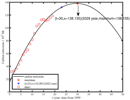
Figure 1. Carbon emission data from 2000 to 2018 and fitting curve.

Therefore, because the meaning of parameter m in model (3) is the maximum peak value of carbon emissions, combined with Figure 1, we take $m=138.135$.

Next, we assume that this year’s natural growth rate is the difference between this year’s carbon emissions and last year’s carbon emissions divided by last year’s carbon emissions, that is, $a_{1,j}=\frac{x_j-x_{j-1}}{x_j}(j=2001,2002,\cdots )$, and we calculated the annual natural growth rate of carbon emissions and simulated it with a first-order function curve. Each blue asterisk in Figure 2 represents the natural growth rate of carbon emissions each year, and the blue line represents the simulation image of a function of these data, as shown in Figure 2.

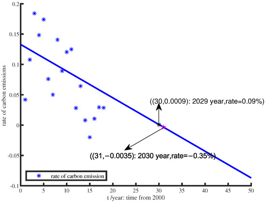
Figure 2. Analysis of the natural growth rate of carbon emissions and fitting curve.

Figure 2 shows that 2029 is the last year when the natural growth rate of carbon emissions is positive with 0.09%, and it turns negative by 2030 with −0.35%.

It is common sense that the maximum capacity of carbon emissions should be greater than the peak of carbon emissions, carbon absorption is the same, so we choose $N_1=2m=276.27,N_2=1.1m=151.9485$, whose units are both ${10}^2$ million ton. Since we chose a competitive model, we chose competition factors of $S_1=2$ and $S_2=0.5$ to make carbon emissions and carbon sequestration competitive. We assume natural growth rate of carbon emissions of between 0.14 and 0.05, thus, we choose $a_1=0.14,a_2=0.2,k=0.5$.

Based on the above analysis, we take one group of parameters as follows,

$$a_1=0.14,a_2=0.2,k=0.5S_1=2S_2=0.5N_1=276.27,N_2=151.9485,m=138.135.$$

5.2. Simulation Results

We select the above group of parameters given in Section 5.1, that is,

$$a_1=0.14,a_2=0.2,k=0.5S_1=2S_2=0.5N_1=276.27,N_2=151.9485,m=138.135.$$

After calculation, we find that the group of parameters satisfies hypothesis conditions $\left(H_1\right)$ and $\left(H_3\right)$, the hypothesis condition $\left(H_2\right)$ is not satisfied, that is, $E_1$ and $E_3$ exist, but $E_2$ does not exist. Since $E_1$ is a boundary equilibrium, we should actually discuss the stability of the non-trivial equilibrium, so we will discuss the stability of the equilibrium $E_3$ in the following part, and $E_3=(119.81,119.82)$; from Equation (17), we calculate that $T_2=0.7365>0,D_2=0.0815>0$. Thus, equilibrium $E_3$ is locally asymptotically stable when $\tau =0$. We select initial value (132, 50), and the simulation result of the stable equilibrium $E_3$ is shown in Figure 3.

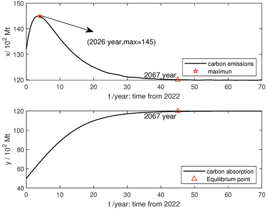
Figure 3. Equilibrium $E_3$ of system (3) is locally asymptotically stable when $\tau =0$.

Remark 2.

From Figure 3, we take $\tau =0$, which indicates that the impact of technological innovation on carbon emissions is instantaneous. We conclude that China will reach the carbon peak in 2026, and the peak value is about 14.5 billion tons. With time going by, the carbon emissions will become smaller and smaller, and gradually reach stability in 2067. The stable value is at about 11.981 billion tons, carbon absorption will increase with time and stabilize at 11.982 billion tons around 2067. For this reason, if China implements the current policy, it will achieve peak carbon dioxide emissions by 2030, but not carbon neutrality by 2060. Therefore, China should adopt stronger policies to lay the foundation for carbon neutrality. In Figure 1, we can see that China’s peak carbon dioxide emissions time is 2029, with a peak value of 13.81 billion tons, while in Figure 3, the simulation results show that China has completed peak carbon dioxide emissions in an earlier time and the peak value will increase. As the coefficients in our model are constant, but in real life, the coefficients of the model may change with time. Another reason is that our model does not consider too many factors, such as the influence of construction industry and carbon sink, which leads to a slight deviation in our simulation results. However, our simulation results are at least consistent with the realization of peak carbon dioxide emissions before 2030.

After that, we consider the time of carbon peak at the difference of the influence factors of industrial structure and energy structure on carbon emissions (see Figure 4).

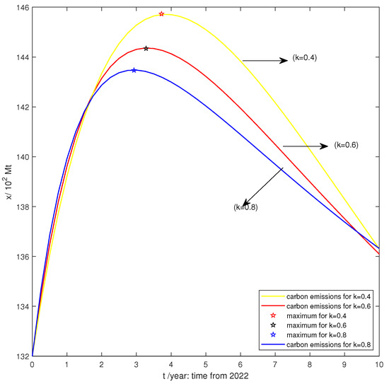
Figure 4. Change of carbon emission under different values for the influence coefficient of energy structure reform on carbon emissions amount k.

Remark 3.

From Figure 4, when the influence coefficient of energy structure reform on carbon emissions amount k increases, that is, with the optimization of industrial structure and the improvement of energy structure, the time for China to reach the carbon peak will become shorter and shorter. When $k=0.4$, we predict that the peak value of carbon will reach 14.573 billion tons in April 2026. When $k=0.6$, China will reach the peak of carbon in April 2025, with a peak of 14.43 billion tons. When $k=0.8$, we predict that China will reach peak carbon dioxide emissions in 2025, with a peak of 14.34 billion tons. This is reasonable because when China’s emission reduction policy is effectively implemented, corresponding policies are introduced, new development of new energy exploration and application technologies is achieved, and industrial reform is conducted in depth. China’s secondary industry with high carbon emissions will be transformed into a green and sustainable tertiary industry in an all-round way. The proportion of clean energy, mainly natural gas, will be greatly increased, and the peak value of carbon emissions will be reduced while reaching the maximum value ahead of time.

Later, we select the previous data, and when the natural growth rate of carbon absorption increases, we arrive at the following conclusions: (see Figure 5).

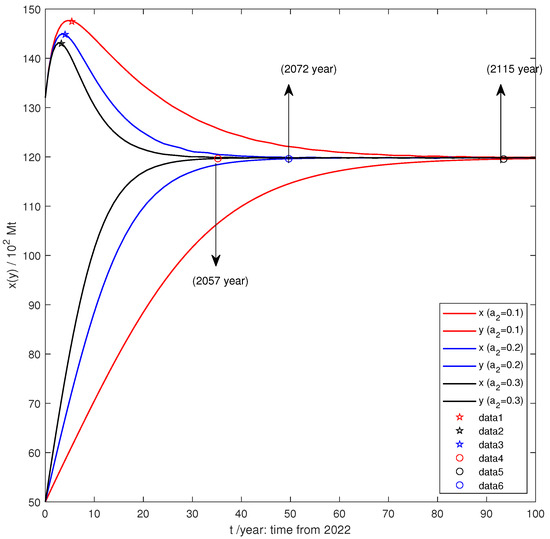
Figure 5. Analysis of the influence of natural growth rate of carbon absorption on carbon absorption and emission.

Remark 4.

With the increase of natural growth rate of carbon absorption, the peak value of carbon emissions becomes smaller and smaller, and the time for carbon to reach the peak value becomes shorter and shorter, and the time for carbon neutrality becomes shorter. The red line in Figure 5 shows the apparent trend of carbon emissions and carbon absorption at $a_2=0.1$. China will reach peak carbon dioxide emissions around 2028, but it will take nearly one hundred years to achieve carbon neutrality. The blue curve shows the change trend of carbon emissions and carbon absorption at $a_2=0.2$, and it is predicted that China will reach peak carbon dioxide emissions around 2026 and be carbon neutral in 2072. The black curve shows the change trend of carbon emissions and carbon absorption at $a_2=0.3$. It can be seen that China will reach peak carbon dioxide emissions around 2026 and become carbon neutral in 2057. Although China can achieve peak carbon dioxide emissions by 2030 at different natural growth rates of carbon absorption, China cannot achieve carbon neutrality by 2060 at a lower natural growth rate of carbon absorption. It also shows that with the country’s emphasis on ecological protection and green development, people have a clearer understanding of green development, saving energy, planting trees, increasing forest vegetation coverage and increasing urban green space, which leads to an increase in the natural growth rate of carbon absorption. The smaller the carbon peak, the shorter the time to achieve carbon neutrality. In Figure 5, we can see that when the natural growth rate of carbon absorption reaches 0.3, it is possible for China to achieve carbon neutrality by 2060. As the natural growth rate of carbon absorption is relatively high, in order to achieve China’s goal of carbon neutrality by 2060, we should not only consider increasing the natural growth rate of carbon absorption to achieve carbon neutrality, but also consider optimizing the industrial structure and energy structure to reduce the natural growth rate of carbon emissions. Therefore, we also need to deepen the industrial reform and optimize the energy structure to reduce the natural growth rate of China’s carbon emissions.

Further on, we find that Formula (22) has only one positive root, so we calculate that ${\tau }_1^{\left(0\right)}=3.606$. From Theorem 3, we know that when $\tau \in [0,{\tau }_1^{\left(0\right)})$, the equilibrium $E_3$ is locally asymptotically stable and unstable when $\tau >{\tau }_1^{\left(0\right)}$. From Equations (37) and (41), we have

$$\mathrm{Re}\left(M\right)=0.1955>0;\mathrm{Re}\left(H\right)=-3.51*{10}^{-7}<0;r=\sqrt{-\frac{\mathrm{Re}\left(M\right)\mu }{\mathrm{Re}\left(H\right)}}>0.$$

(44)

When $\tau =0.5<{\tau }_1^{\left(0\right)}=3.606$, the simulation result of the stable equilibrium $E_3$ is as shown in Figure 6.

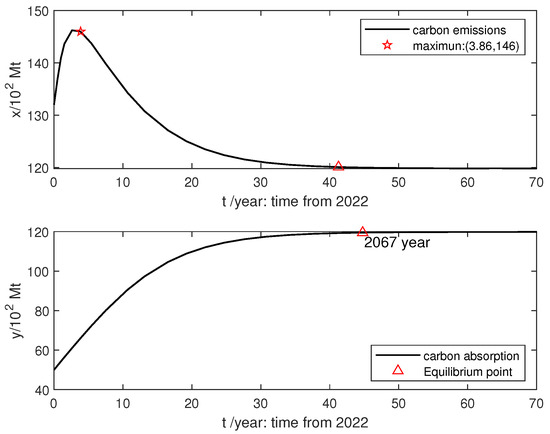
Figure 6. When $\tau =0.5$, the system (3) is locally asymptotically stable at the equilibrium point $E_3$.

Remark 5.

From Figure 6, carbon emissions x reached their peak around 2060, with a peak of about 14.6 billion tons, and then decreased year by year and gradually stabilized, and they became stable around 2063. Carbon absorption y tends to be stable around 2067. Once carbon emissions and carbon absorption are stable, the value of carbon emissions is about 11.9 billion tons, and the value of carbon absorption is about 12 billion tons. If this continues, it will be difficult for China to achieve carbon neutrality before 2060. Therefore, China needs to take some measures, such as improving the level of carbon emission reduction technology to reduce the carbon emissions of the steel industry.

When $\tau =3.61>{\tau }_1^{\left(0\right)}=3.606$, from Theorem 4, we learn that the system (3) has a stable periodic solution at the at the equilibrium $E_3$, as shown in Figure 7.

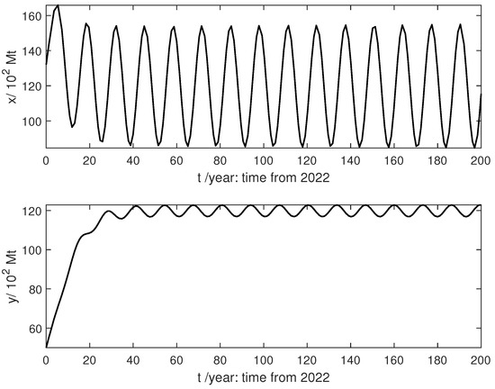
Figure 7. When $\tau =3.61$, the system (3) has a stable periodic solution near the equilibrium $E_3$.

Remark 6.

From Figure 7, when $\tau =3.61$, the system (3) is locally asymptotically stable at the equilibrium $E_3$, which is consistent with (4). $\tau =3.61$, that is, when the technical level is applied to the actual production of carbon emission reduction, the time required becomes longer, we can see that carbon emissions and carbon absorption fluctuate periodically, and the period is about 13 years. As a result of the long delay time, it is inconsistent with the actual production level at present, so we do not consider the practical application of this situation.

6. Conclusions

In this paper, considering the competitive relationship between carbon emission and carbon absorption, we set up a new two-dimensional differential equation model with time delay to make some predictions and analyze whether China can achieve it under the current policy, which depends on China’s technology research and development level and government policy investment. In practice, the parameters of the model are variable. In order to simplify the problem, the parameters of the model (3) are constant coefficients. At the same time, the model in this paper does not consider too many factors. The simulation process of the model may be different from the real process. For example, the peak value of the simulation will be higher than the future peak value because we have not fully considered the carbon emission reduction measures, but on the whole, the stability of our model is consistent with the actual one. In addition, we theoretically analyzed the existence and stability of the equilibrium and the existence of Hopf bifurcation, and we also derive the normal form of Hopf bifurcation for the system (3) by using the multiple time scales method. After that, we selected a set of data for numerical analysis to verify our theoretical analysis results, we find that equilibrium $E_3$ of system (3) is locally asymptotically stable when $\tau =0$. When $\tau =3.61$, the system (3) has a stable periodic solution near the equilibrium $E_3$ and we find from Figure 4 that the optimization and adjustment of industrial structure and energy structure has an important impetus to China’s realization of peak carbon dioxide emissions and carbon neutrality. When the industrial structure is optimized and the energy structure is improved, the time for China to reach peak carbon dioxide emissions will be shortened (see Figure 4).

Next, our numerical analysis also shows that when the natural growth rate of carbon absorption increases, the time for China to achieve carbon peak carbon dioxide emissions will be shortened and the peak value will also decrease (see from Figure 5). From Figure 5, we predict that when the natural growth rate of carbon absorption is 0.3, China will achieve carbon neutrality before 2060. As the natural growth rate of carbon absorption is actually too high, we also need to deepen the industrial reform and optimize the energy structure to reduce the natural growth rate of China’s carbon emissions. Therefore, based on the above research, this paper emphasizes planting trees and improving the level of carbon storage technology to improve the natural growth rate of carbon absorption and carbon emission reduction technology, and improving the development and application technology of new energy to achieve in-depth industrial structure adjustment and energy structure optimization. The above measures are of great significance to China’s realization of peak carbon dioxide emissions by 2030 and carbon neutrality by 2060.

References

- Zhang, G.X.; Zhang, P.D.; Xiu, J.; Chai, J. Are energy conservation and emission reduction policy measures effective for industrial structure restructuring and upgrading? Chin. J. Popul. Resour. 2018, 1, 12–27. [Google Scholar] [CrossRef]
- Cai, B.F.; Wang, J.N.; Yang, S.Y.; Mao, Y.Q.; Cao, L.B. Carbon dioxide emissions from cities in China based on high resolution emission gridded data. Chin. J. Popul. Resour. 2017, 15, 58–70. [Google Scholar] [CrossRef]
- Zou, C.N.; Xiong, B.; Xue, H.Q.; Zheng, D.W.; Ge, Z.X.; Wang, Y.; Jiang, L.Y.; Pan, S.Q.; Wu, S.D. The role of new energy in carbon neutral. Petrol. Explor. Dev. 2021, 48, 480–491. [Google Scholar] [CrossRef]
- Zhang, Y.X.; Yin, J.P.; Fu, Y.; Wang, J.X.; Wang, G.S. The research of carbon emission and carbon sequestration potential of forest vegetation in China. Meteorol. Environ. Res. 2021, 12, 24–31. [Google Scholar]
- Du, X.W. China’s low-carbon transition for addressing climate change. Adv. Clim. Chang. Res. 2016, 1, 105–108. [Google Scholar] [CrossRef]
- Feng, X.P. Carbon dioxide emissions reduction technology and its application prospects in the steel industry. Baosteel Tech. Res. 2010, s1, 131. [Google Scholar]
- Feng, R.; Dai, B.Z.; Su, H. Effect of China’s industrial structure adjustment on carbon emissions. Ecol. Econ. 2017, 2, 117–124. [Google Scholar]
- Wang, S.J.; Gao, S.; Huang, Y.Y.; Shi, C.Y. Spatiotemporal evolution of urban carbon emission performance in China and prediction of future trends. Acta Geogr. Sin. 2020, 30, 757–774. [Google Scholar] [CrossRef]
- Chen, J.H. An empirical study on China’s energy supply-and-demand model considering carbon emission peak constraints in 2030. Engineering 2017, 3, 512–517. [Google Scholar] [CrossRef]
- Guo, C.X. Estimation of emission reduction potential in China’s industrial sector. Chin. J. Popul. Resour. 2015, 3, 223–230. [Google Scholar] [CrossRef]
- Li, S.Q.; Zhang, B.S.; Tang, X. Forecasting of China’s natural gas production and its policy implications. Petrol. Sci. 2016, 13, 592–603. [Google Scholar] [CrossRef]
- Muhammad, K.K.; Muhammad, I.K.; Muhammad, R. The relationship between energy consumption, economic growth and carbon dioxide emissions in Pakistan. Financ. Innov. 2020, 6, 56–68. [Google Scholar]
- Liu, K.; Tao, Y.M.; Wu, Y.; Wang, C.X. How does ecological civilization construction affect carbon emission intensity? Evidence from Chinese provinces’panel data. Chin. J. Popul. Resour. 2020, 18, 97–102. [Google Scholar]
- Sahoo, D.; Samanta, G.P. Comparison between two tritrophic food chain models with multiple delays and anti-predation effect. Int. J. Biomath. 2021, 14, 53–100. [Google Scholar] [CrossRef]
- Khajanchi, S. Chaotic dynamics of a delayed tumor immune interaction model. Int. J. Biomath. 2020, 13, 1–33. [Google Scholar] [CrossRef]
- Tessema, M.K.; Chirove, F.; Sibanda, P. Modeling control of foot and mouth disease with two time delays. Int. J. Biomath. 2019, 12, 1–37. [Google Scholar] [CrossRef]
- Ren, H.P.; Li, W.C.; Liu, D. Hopf bifurcation analysis of Chen circuit with direct time delay feedback. Chin. Phys. B 2010, 3, 164–175. [Google Scholar]
- Zhang, M.M.; Wang, C.J.; Mei, D.C. Effect of time delay on the upper bound of the time derivative of information entropy in a stochastic dynamical. Chin. Phys. B 2011, 20, 122–126. [Google Scholar] [CrossRef]
- Orosz, G. Hopf bifurcation calculations in delayed systems. Mech. Eng. 2004, 48, 189–200. [Google Scholar]
- Awang, N.A.; Maan, N.; Sulain, M.D. Tumour-natural killer and cD8+ t cells interaction model with delay. Mathematics 2022, 10, 2193. [Google Scholar] [CrossRef]
- Liu, X.; Ding, Y. Stability and numerical simulations of a new SVIR model with two delays on COVID-19 booster vaccination. Mathematics 2022, 10, 1772. [Google Scholar] [CrossRef]
- Wang, J.; Wang, Y. Study on the stability and entropy complexity of an energy-saving and emission-reduction model with two delays. Entropy 2016, 18, 371. [Google Scholar] [CrossRef]
- Nayfeh, A.H. Order reduction of retarded nonlinear systems—The method of multiple scales versus center-manifold reduction. Nonlin. Dyn. 2008, 51, 483–500. [Google Scholar] [CrossRef]
- Das, S.L.; Chatterjee, A. Multiple scales without center manifold reductions for delay differential equations near Hopf bifurcations. Nonlin. Dyn. 2002, 30, 323–335. [Google Scholar] [CrossRef]
Publisher’s Note: MDPI stays neutral with regard to jurisdictional claims in published maps and institutional affiliations. |
© 2022 by the authors. Licensee MDPI, Basel, Switzerland. This article is an open access article distributed under the terms and conditions of the Creative Commons Attribution (CC BY) license (https://creativecommons.org/licenses/by/4.0/).