Statistical Inference on a Finite Mixture of Exponentiated Kumaraswamy-G Distributions with Progressive Type II Censoring Using Bladder Cancer Data

Abstract

A new family of distributions called the mixture of the exponentiated Kumaraswamy-G (henceforth, in short, ExpKum-G) class is developed. We consider Weibull distribution as the baseline (G) distribution to propose and study this special sub-model, which we call the exponentiated Kumaraswamy Weibull distribution. Several useful statistical properties of the proposed ExpKum-G distribution are derived. Under the classical paradigm, we consider the maximum likelihood estimation under progressive type II censoring to estimate the model parameters. Under the Bayesian paradigm, independent gamma priors are proposed to estimate the model parameters under progressive type II censored samples, assuming several loss functions. A simulation study is carried out to illustrate the efficiency of the proposed estimation strategies under both classical and Bayesian paradigms, based on progressively type II censoring models. For illustrative purposes, a real data set is considered that exhibits that the proposed model in the new class provides a better fit than other types of finite mixtures of exponentiated Kumaraswamy-type models.

1. Introduction

The utility of mixture distributions during the last decade or so have provided a mathematical-based strategy to model a wide range of random phenomena effectively. Statistically speaking, the mixture distributions are a useful tool and have greater flexibility to analyze and interpret the probabilistic alias random events in a possibly heterogenous population. In modeling real-life data, it is quite normal to observe that the data have come from a mixture population involving of two or more distributions. One may find ample evidence(s) in terms of applications of finite mixture models not limited to but including in medicine, economics, psychology, survival data analysis, censored data analysis and reliability, among others. In this article, we are going to explore such a finite mixture model based on bounded (on (0,1)) univariate continuous distribution mixing with another baseline (G) continuous distribution and will study its structural properties with some applications. Next, we provide some useful references related to finite mixture models that are pertinent in this context. Ref. [1] introduced the classical and Bayesian inference on the finite mixture of exponentiated Kumaraswamy Gompertz and exponentiated Kumaraswamy Fréchet (MEKGEKF) distributions under progressively type II censoring with applications and it appears that this MEKGEKF distribution might be useful in analyzing certain dataset(s), for which either or both of its component distributions will be inadequate to completely explain the data. Consequently, this also serves as one of the main purposes for the current work.

In recent years, there has been a lot of interest in the art of parameter(s) induction to a baseline distribution. The addition of one or more extra shape parameter(s) to the baseline distribution makes it more versatile, particularly for examining the tail features. This parameter(s) induction also improved the goodness-of-fit of the proposed generalized family of distributions, despite the computational difficulty in some cases. Over two decades, there have been numerous generalized G families of continuous univariate distributions that have been derived and explored to model various types of data adequately. The exponentiated family, Marshall–Olkin extended family, beta-generated family, McDonald-generalized family, Kumaraswamy-generalized family, and exponentiated generalized family are among the well-known and widely recognized G families of distributions that are addressed in [2]. Some Marshall–Olkin extended variants and the Kumaraswamy-generalized family of distributions are proposed. For the exponentiated Kumaraswamy distribution and its log-transform, one can refer to [3]. Refs. [4,5] defined the probability density function (pdf) of exponentiated Kumaraswamy G (henceforth, in short, EKG) distributions, which is as follows:

$$f\left(x\right)=abcg\left(x\right)G^{a-1}\left(x\right){\left[1-G^a\left(x\right)\right]}^{b-1}{\left\{1-{\left[1-G^a\left(x\right)\right]}^b\right\}}^{c-1}$$

(1)

where $a,b,c$ are all positive parameters and $x>0$.

The associated cumulative distribution function (cdf) is given by

$$F\left(x\right)={\left\{1-{\left[1-G^a\left(x\right)\right]}^b\right\}}^c, x>0.$$

If $u\in \left(0,1\right),$ the associated quantile function is given by

$$x\left(u\right)=G^{-1}{\left\{1-{\left[1-u^{\frac{1}{c}}\right]}^{\frac{1}{b}}\right\}}^{\frac{1}{a}}$$

(2)

In this paper, we consider a finite mixture of two independent EKW distributions with mixing weights and consider an absolute continuous probability model, namely the two-parameter Weibull, as a baseline model.

The rest of this article is organized as follows. In Section 2, we provide the mathematical description of the proposed model. In Section 3, some useful structural properties of the proposed model are discussed. The maximum likelihood function of the mixture exponentiated Kumaraswamy-G distribution based on progressively type II censoring is given in Section 4. Section 5 deals with the specific distribution of the mixture of exponentiated Kumaraswamy-G distribution when the baseline (G) is a two parameter Weibull, henceforth known as EKW distribution. In Section 6, we provide a general framework for the Bayes estimation of the vector of the parameters and the posterior risk under different loss functions of the exponentiated Kumaraswamy-G distribution. In Section 7, we consider the estimation of the EKW distribution under both the classical and Bayesian paradigms via a simulation study and under various censoring schemes. For illustrative purposes, an application of the EKW distribution is shown by applying the model to bladder cancer data in Section 8. Finally, some concluding remarks are presented in Section 9.

2. Model Description

A density function of the mixture of two components’ densities with mixing proportions $p\in \left[0,1\right]$ and $q=1-p$ of EKG distributions is given as follows:

$$f\left(x\right)=p{f}_1\left(x\right)+q{f}_2\left(x\right),$$

where

$$f_j\left(x\right)=a_j{b}_j{c}_{j}g\left(x\right)G^{a_j-1}\left(x\right){\left[1-G^{a_j}\left(x\right)\right]}^{b_j-1}{\left\{1-{\left[1-G^{a_j}\left(x\right)\right]}^{b_j}\right\}}^{c_j-1}$$

for $x>0,$ with $a_j{b}_j{c}_j>0,$ and $j=1,2,$ the j-th component and the pdf of the mixture of the two EKG distributions is given by

$$\begin{array}{l}f\left(x\right)=p{a}_1{b}_1{c}_{1}g\left(x\right)G^{a_1-1}\left(x\right){\left[1-G^{a_1}\left(x\right)\right]}^{b_1-1}{\left\{1-{\left[1-G^{a_1}\left(x\right)\right]}^{b_1}\right\}}^{c_1-1}+q{a}_2{b}_2{c}_{2}g\left(x\right)G^{a_2-1}\left(x\right)\\ {\left[1-G^{a_2}\left(x\right)\right]}^{b_2-1}{\left\{1-{\left[1-G^{a_2}\left(x\right)\right]}^{b_2}\right\}}^{c_2-1} I\left(0<x<\infty \right),\end{array}$$

(3)

meaning the associated cdf of the distribution is

$$F\left(x\right)=p{F}_1\left(x\right)+q{F}_2\left(x\right)$$

$$i.e.,F\left(x\right)=p{\left\{1-{\left[1-G^{a_1}\left(x\right)\right]}^{b_1}\right\}}^{c_1}+q{\left\{1-{\left[1-G^{a_2}\left(x\right)\right]}^{b_2}\right\}}^{c_2}, x>0.$$

(4)

The component wise cdf can be obtained as

$$F_j\left(x\right)={\left\{1-{\left[1-G^{a_j}\left(x\right)\right]}^{b_j}\right\}}^{c_j}, x>0.$$

For the density in Equation (3),$\left(a_1,b_1\right), \left(a_2,b_2\right),$ are all playing the role of shape parameters. Consequently, for the varying choices of $a_1,b_1$, $a_2$ and $b_2$ one may obtain various possible shapes of the pdf, as well as for the hrf function.

3. Structural Properties

We begin this section by discussing the asymptotes and shapes of the proposed mixture model in Equation (3).

• Result 1: Shapes. The cdf in Equation (3) can be obtained analytically. The critical points of the pdf are the roots of the following equation:

$$\begin{gathered} \frac{\partial }{\partial x}\left[p{a}_1{b}_1{c}_{1}g\left(x\right)G^{a_1-1}\left(x\right){\left[1-G^{a_1}\left(x\right)\right]}^{b_1-1}{\left\{1-{\left[1-G^{a_1}\left(x\right)\right]}^{b_1}\right\}}^{c_1-1} \\ +q{a}_2{b}_2{c}_{2}g\left(x\right)G^{a_2-1}\left(x\right){\left[1-G^{a_2}\left(x\right)\right]}^{b_2-1}{\left\{1-{\left[1-G^{a_2}\left(x\right)\right]}^{b_2}\right\}}^{c_2-1}\right]=0, \\ =p{a}_1{b}_1{c}_1\left[A_1\left(x\right)\right]+\left(1-p\right)a_2{b}_2{c}_2\left[A_2\left(x\right)\right]=0, \end{gathered}$$

(5)

where

$$\begin{gathered} A_1\left(x\right)=\acute{g}\left(x\right)G^{a_1-1}\left(x\right){\left[1-G^{a_1}\left(x\right)\right]}^{b_1-1}{\left\{1-{\left[1-G^{a_1}\left(x\right)\right]}^{b_1}\right\}}^{c_1-1} \\ +g\left(x\right)\left(a_1-1\right)G^{a_1-2}\left(x\right)g\left(x\right){\left[1-G^{a_1}\left(x\right)\right]}^{b_1-1}{\left\{1-{\left[1-G^{a_1}\left(x\right)\right]}^{b_1}\right\}}^{c_1-1}, \\ =a_1\left(b_1-1\right)g\left(x\right)G^{a_1-1}\left(x\right){\left[1-G^{a_1}\left(x\right)\right]}^{b_1-2}g\left(x\right){\left\{1-{\left[1-G^{a_1}\left(x\right)\right]}^{b_1}\right\}}^{c_1-1} \\ +g\left(x\right)G^{a_1-1}\left(x\right)g\left(x\right){\left[1-G^{a_1}\left(x\right)\right]}^{b_1-1}\left(c_1-1\right){\left\{1-{\left[1-G^{a_1}\left(x\right)\right]}^{b_1}\right\}}^{c_1-2}\left\{b_1{\left[1-G^{a_1}\left(x\right)\right]}^{b_1-1}\right\}{a}_1 \\ g\left(x\right)G^{a_1}\left(x\right), \\ =G^{a_1-1}\left(x\right){\left[1-G^{a_1}\left(x\right)\right]}^{b_1-1}g\left(x\right){\left\{1-{\left[1-G^{a_1}\left(x\right)\right]}^{b_1}\right\}}^{c_1-1} \\ \left\{\left(a_1-1\right)\frac{g^2\left(x\right)}{G\left(x\right)}-\frac{a_1\left(b_1-1\right)g^2\left(x\right)G^{a_1-1}\left(x\right)}{\left[1-G^{a_1}\left(x\right)\right]}+\frac{a_1{b}_1\left(c_1-1\right)g^2\left(x\right)G^{a_1-1}\left(x\right){\left[1-G^{a_1}\left(x\right)\right]}^{b_1-1}}{1-{\left[1-G^{a_1}\left(x\right)\right]}^{b_1}}\right\}, \end{gathered}$$

Similarly,

$$\begin{array}{l}{A}_2\left(x\right)=G^{a_2-1}\left(x\right){\left[1-G^{a_2}\left(x\right)\right]}^{b_2-1}{\left\{1-{\left[1-G^{a_2}\left(x\right)\right]}^{b_2}\right\}}^{c_2-1}\\ \left\{\left(a_2-1\right)\frac{g^2\left(x\right)}{G\left(x\right)}-\frac{a_2\left(b_2-1\right)g^2\left(x\right)G^{a_2-1}\left(x\right)}{\left[1-G^{a_2}\left(x\right)\right]}+\frac{a_2{b}_2\left(c_2-1\right)g^2\left(x\right)G^{a_2-1}\left(x\right){\left[1-G^{a_2}\left(x\right)\right]}^{b_2-1}}{1-{\left[1-G^{a_2}\left(x\right)\right]}^{b_2}}\right\},\end{array}$$

There may be more than one root to the Equation (5). If x = x* is the root of the equation, it corresponds to a local maximum, or a local minimum or a point of inflexion depending on $\xi \left(x^{*}\right)<0, \xi \left(x^{*}\right)=0, or \xi \left(x^{*}\right)>0,$ where $\xi \left(x^{*}\right)=\frac{{\partial }^2}{\partial x^2}\left[f\left(x\right)\right]|x=x^{*}$.

• Result 2: Mixture Representation

A random variable is said to have the exponentiated-G distribution with parameter $a>0$ if $y~Exp-G\left(a\right)$ and if its pdf and cdf is given by $f\left(y\right)=a g\left(x\right)G^a\left(x\right)$ and $F\left(y\right)=G^a\left(x\right)$, as shown in [6,7].

If one considers the following, we have the following equations:

$$\begin{gathered} f_1\left(x\right)=a_1{b}_1{c}_{1}g\left(x\right)G^{a_1-1}\left(x\right){\left[1-G^{a_1}\left(x\right)\right]}^{b_1-1}{\left\{1-{\left[1-G^{a_1}\left(x\right)\right]}^{b_1}\right\}}^{c_1-1} \\ =a_1{b}_1{c}_{1}g\left(x\right)G^{a_1-1}\left(x\right){\left[1-G^{a_1}\left(x\right)\right]}^{b_1-1}{\displaystyle \sum }_{j_1=0}^{\infty }{\left(-1\right)}^{j_1}\left(\begin{array}{c}{c}_1-1\\ j_1\end{array}\right){\left[1-G^{a_1}\left(x\right)\right]}^{j_1{b}_1} \\ =a_1{b}_1{c}_1{\displaystyle \sum }_{j_1=0}^{\infty }{\left(-1\right)}^{j_1}{\displaystyle \sum }_{j_2=0}^{\infty }{\left(-1\right)}^{j_2}\left(\begin{array}{c}{c}_1-1\\ j_1\end{array}\right)\left(\begin{array}{c}{b}_1(j_1+1)-1\\ j_2\end{array}\right)g\left(x\right)G^{a_1-1}\left(x\right)G^{a_1{j}_2}\left(x\right), \\ =a_1{b}_1{c}_1{\displaystyle \sum }_{j_1=0}^{\infty }{\displaystyle \sum }_{j_2=0}^{\infty }{\left(-1\right)}^{j_1+j_2}\frac{\left(\begin{array}{c}{c}_1-1\\ j_1\end{array}\right)\left(\begin{array}{c}{b}_1(j_1+1)-1\\ j_2\end{array}\right)}{a_1(j_2+1)}{G}^{a_1\left(j_2+1\right)}\left(x\right). \end{gathered}$$

Likewise,

$$f_2\left(x\right)=a_2{b}_2{c}_2{{\displaystyle \sum }}_{j_1=0}^{\infty }{{\displaystyle \sum }}_{j_2=0}^{\infty }{\left(-1\right)}^{j_1+j_2}\frac{\left(\begin{array}{c}{c}_2-1\\ j_1\end{array}\right)\left(\begin{array}{c}{b}_2(j_2+1)-1\\ j_2\end{array}\right)}{a_2(j_2+1)}{G}^{a_2\left(j_2+1\right)}\left(x\right).$$

Therefore,

$$\begin{gathered} f\left(x\right)=p{\left(a_2{b}_2{c}_2\right)}^{-1}{{\displaystyle \sum }}_{j_1=0}^{\infty }{{\displaystyle \sum }}_{j_2=0}^{\infty }{\mathsf{\Psi }}_1\left(j_1,j_2,b_1,c_1\right)G^{a_1\left(j_2+1\right)}\left(x\right)+ \\ q{\left(a_2{b}_2{c}_2\right)}^{-1}{{\displaystyle \sum }}_{j_1=0}^{\infty }{{\displaystyle \sum }}_{j_2=0}^{\infty }{\mathsf{\Psi }}_2\left(j_1,j_2,b_2,c_2\right)G^{a_2\left(j_2+1\right)}\left(x\right) \end{gathered}$$

where ${\mathsf{\Psi }}_1\left(j_1,j_2,b_1,c_1\right)=\frac{{\left(-1\right)}^{j_1+j_2}}{a_1(j_2+1)}\left(\begin{array}{c}{c}_1-1\\ j_1\end{array}\right)\left(\begin{array}{c}{b}_1(j_1+1)-1\\ j_2\end{array}\right)$ and ${\mathsf{\Psi }}_2\left(j_1,j_2,b_2,c_2\right)=\frac{{\left(-1\right)}^{j_1+j_2}}{a_2(j_2+1)}\left(\begin{array}{c}{c}_2-1\\ j_1\end{array}\right)\left(\begin{array}{c}{b}_2(j_2+1)-1\\ j_2\end{array}\right).$

Note that if $b_1$, $c_1$, $b_2,$ $c_2$ are integers, then the repective sums will stop at $b_1$, $c_1$, $b_2$ and $c_2$.

The above expression shows the fact that the pdf of the finite mixture of EKG can be represented as the finite mixture of infinite exponentiated-G distribution with parameters $a_1(j_2+1)$ and $a_2(j_2+1)$, respectively.

Therefore, structural properties, such as moments, entropy, etc., of this model can be obtained from the knowledge of the exponentiated-G distribution and one can refer to [8] for some pertinent details.

• Result 3: Simulation Strategy

Method 1. Direct cdf inversion method

Step 1: Generate $U~Uniform \left(0,1\right).$

Step 2: Then, set $X_i=p_i{\left\{1-{\left[1-U_i^{\frac{1}{c_i}}\right]}^{\frac{1}{b_i}}\right\}}^{\frac{1}{a_i}}, {\displaystyle \sum }_{i=1}^2{p}_i=1,for\left(a_i,b_i,c_i\right)>0 \forall i=1,2$.

Method 2. Via acceptance-rejection sampling plan

This will work if $a\ge 1, b\ge 1, c\ge 1$.

One must define $D_1=\frac{a_1^{b_1{c}_1}{b}_1{\left(a_1-1\right)}^{1-\frac{1}{a_1}}{\left(b_1-1\right)}^{b_1-1}{\left(c_1-1\right)}^{c_1-1}}{{\left(a_1{b}_1{c}_1-1\right)}^{c_1-\frac{1}{a_1{b}_1}}}$

and $D_2=\frac{a_2^{b_2{c}_2}{b}_2{\left(a_2-1\right)}^{1-\frac{1}{a_2}}{\left(b_2-1\right)}^{b_2-1}{\left(c_2-1\right)}^{c_2-1}}{{\left(a_2{b}_2{c}_2-1\right)}^{c_2-\frac{1}{a_2{b}_2}}}.$

$M=max\left\{D_1,D_2\right\}.$ Then, the following scheme will work:

(i)

Simulate $X=x$ from the pdf in Equation (3).

(ii)

Simulate $Y=UMg\left(x\right)$, where $U~Uniform \left(0,1\right)$.

(iii)

Accept $X=x$ as a sample from the target density if $y<f\left(x\right).$ If $y\ge f\left(x\right),$ one must go to step (ii).

One may obtain an expression of the reliability function of mixture EKG, which takes the following form:

$$R\left(x\right)=p{R}_1\left(x\right)+q{R}_2\left(x\right)$$

where the component-wise reliability function of the mixture model is given by

$$R_j\left(x\right)=1-{\left\{1-{\left[1-G^{a_j}\left(x\right)\right]}^{b_j}\right\}}^{c_j}, x>0.$$

The density in Equation (1) is flexible in the sense that one can obtain different shapes of hazard rate function (hrf) of the mixture model, which is given by

$$h_j\left(x\right)=\frac{a_j{b}_j{c}_{j}g\left(x\right){\left[1-G^{a_j}\left(x\right)\right]}^{b_j-1}{\left\{1-{\left[1-G^{a_j}\left(x\right)\right]}^{b_j}\right\}}^{c_j-1}}{1-{\left\{1-{\left[1-G^{a_j}\left(x\right)\right]}^{b_j}\right\}}^{c_j}}.$$

The quantile function of the mixture model is given by

$$q\left(x\right)=p{G}^{-1}{\left\{1-{\left[1-U^{\frac{1}{c_1}}\left(x\right)\right]}^{\frac{1}{b_1}}\right\}}^{\frac{1}{a_1}}+q{G}^{-1}{\left\{1-{\left[1-U^{\frac{1}{c2}}\left(x\right)\right]}^{\frac{1}{b_2}}\right\}}^{\frac{1}{a_2}}.$$

For example, the median, $x_m$, of $f\left(x\right)$ for $U=0.5$ will be

$$x_m=p{G}^{-1}{\left\{1-{\left[1-{0.5}^{\frac{1}{c_1}}\left(x\right)\right]}^{\frac{1}{b_1}}\right\}}^{\frac{1}{a_1}}+q{G}^{-1}{\left\{1-{\left[1-{0.5}^{\frac{1}{c2}}\left(x\right)\right]}^{\frac{1}{b_2}}\right\}}^{\frac{1}{a_2}},$$

The various shapes of the pdf and the hrf when the baseline distribution (G) is Weibull is provided in Figure 1. In the next section, we discuss the maximum likelihood estimation strategy for the finite mixture of exponentiated Kumaraswamy-G (EKG) distribution under the progressive type-II censoring scheme. For more details, one can refer to [9]. The necessary and sufficient conditions for identifiability and identifiability properties are discussed in the Appendix A.

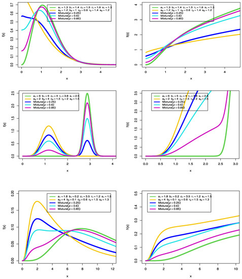
Figure 1. The pdf and hrf of the MEKW model for different values of its parameters.

4. Maximum Likelihood Estimation of EKG Distribution under Progressive Type-II Censoring

One must suppose that n units are put on life test at time zero and the experimenter decides beforehand the quantity m, the number of failures to be observed. At the time of first failure, $R_1$ units are randomly removed from the remaining n-1 surviving units. At the second failure, $R_2$ units from the remaining $n-2-R_1$ units are randomly removed. The test continues until the mth failure. At this time, all remaining $R_m=n-m-R_1-R_2-\dots -R_{m-1}$ units are removed. In this censoring scheme, $R_i$ and m are prefixed. The resulting m is ordered. Values, which are obtained as a consequence of this type of censoring, are appropriately referred to as progressive type II censored ordered statistics. One must note that if $R_1=R_2=\dots =R_{m-1}=0,$ so that $R_m=n-m$, this scheme reduces to a conventional type II on the stage right censoring scheme.

One must also note that if $R_1=R_2=\dots =R_m=0,$ so that m = n, the progressively type II censoring scheme reduces to the case of a complete sample (the case of no censoring).

One must allow ($X_{1:m:n},X_{2:m:n},\dots ,X_{m:m:n})$ to be a progressively type II censored sample, with $\left(R_1,R_2,\dots ,R_m\right)$ being the progressive censoring scheme. The likelihood function based on the progressive censored sample of EKG distributions is given by

$$L\left(\underset{\_}{x} |a_j,b_j,c_j,s_j,r_j,p,q\right)=K{{\displaystyle \prod }}_{i=1}^{m}g\left(X_{i:m:n}\right){\left[1-G\left(X_{i:m:n}\right)\right]}^{R_i}$$

where $k=n\left(n-1-R_1\right)\left(n-1-R_2\right)\dots \left(n-m+1-R_1\dots -R_m\right)$, g(x) and G(x) are given in Equations (3) and (4) and we obtain the log likelihood function without the constant term, which is is given by

$$L\left(\underset{\_}{x} |a_j,b_j,c_j,s_j,r_j,p,q\right)\propto {{\displaystyle \prod }}_{i=1}^m{g}_j\left(X_{i:m:n}\right){\left[1-G_j\left(X_{i:m:n}\right)\right]}^{R_i}$$

To simplify, we take the logarithm of the likelihood function, $ı,$ and for illustration purposes, let $g_j\left(X_{i:m:n}\right)=f_j\left(X_{i:m:n}\right)$ and $G_j\left(X_{i:m:n}\right)=F_j\left(X_{i:m:n}\right)$ as follows:

$$ı\propto {{\displaystyle \sum }}_{i=1}^{m}log\left[f_j\left(X_{i:m:n}\right)\right]+R_{i}log\left[1-F_j\left(X_{i:m:n}\right)\right]$$

Next, for illustrative purposes, we consider the baseline (G) distribution to be a two parameter Weibull distribution on the EKG distribution and discuss its estimation under both the classical and Bayesian set up.

5. Finite Mixture of Exponentiated Kumaraswamy Weibull Distribution

Exponentiated Kumaraswamy Weibull (EKW) distribution is a special case that can be generated from exponentiated Kumaraswamy -G distributions. The EKW distribution is found by taking G(x) of the Weibull distribution in Equation (1). One of the most important advantages of the EKW distribution is its capacity to fit data sets with a variety of shapes, as well as for censored data, compared to the component distributions. One must let G be the Weibull distribution with the pdf and the cdf are given by

$$g\left(x\right)=\frac{r}{s}{\left(\frac{x}{s}\right)}^{r-1}exp\left[-{\left(\frac{x}{s}\right)}^r\right],x>0,$$

and

$$G\left(x\right)=\left(1-exp\left[-{\left(\frac{x}{s}\right)}^r\right]\right).$$

The inverse of the cdf is given by

$$s{\left(-ln\left(1-G\left(u\right)\right)\right)}^{\frac{1}{r}}=Q\left(u\right)$$

The pdf of a mixture of two component densities with mixing proportions, ($p_j, j=1,2)$ for q = 1 − p of the exponentiated Kumaraswamy Weibull distribution (henceforth, in short is MKEW) is given by

$$\begin{array}{l}f\left(x\right)=p\frac{a_1{b}_1{c}_1{r}_1}{s_1}{\left(\frac{x}{s_1}\right)}^{r_1-1}exp\left[-{\left(\frac{x}{s_1}\right)}^{r_1}\right]{\left[1-exp\left(-{\left(\frac{x}{s_1}\right)}^{r_1}\right)\right]}^{a_1-1}{\left[1-{\left[1-exp\left(-{\left(\frac{x}{s_1}\right)}^{r_1}\right)\right]}^{a_1}\right]}^{b_1-1}\\ {\left[1-{\left[1-{\left[1-exp\left(-{\left(\frac{x}{s_1}\right)}^{r_1}\right)\right]}^{a_1}\right]}^{b_1}\right]}^{c_1-1}+q\frac{a_2{b}_2{c}_2{r}_2}{s_2}{\left(\frac{x}{s_2}\right)}^{r_2-1}exp\left[-{\left(\frac{x}{s_2}\right)}^{r_2}\right]{\left[1-exp\left(-{\left(\frac{x}{s_2}\right)}^{r_2}\right)\right]}^{a_2-1}\\ {\left[1-{\left[1-exp\left(-{\left(\frac{x}{s_2}\right)}^{r_2}\right)\right]}^{a_2}\right]}^{b_2-1}{\left[1-{\left[1-{\left[1-exp\left(-{\left(\frac{x}{s_2}\right)}^{r_2}\right)\right]}^{a_2}\right]}^{b_2}\right]}^{c_2-1}, x>0\end{array}$$

(6)

For the pdf in Equation (6), the following is noted:

(i)

$s_1 \mathrm{and}$ $s_2$ are the scale parameters and $r_1 \mathrm{and}$ $r_2$ are the shape parameters for the Weibull component.

(ii)

$a_1, a_2, b_1 \mathrm{and} b_2$, are the shape parameters arising from the finite mixture pdf in Equation (4);

(iii)

$p, \mathrm{and} q$ are the mixing proportions ,where $p+q=1$.

Depending on the different values of the parameters, different shapes of the pdf and the hrf of the MEKW distribution are shown in Figure 1. From Figure 1 (left panel), it appears that the MEKW pdf can include symmetric, asymmetric, right-skewed, and decreasing shapes, depending on the values of parameters. From Figure 1 (right panel), one can observe that the hrf may assume shapes with constants and that are down-upward and increasing.

The associated cdf is given by

$$F\left(x\right)=p{\left[1-{\left[1-{\left[1-exp\left(-{\left(\frac{x}{s_1}\right)}^{r_1}\right)\right]}^{a_1}\right]}^{b_1}\right]}^{c_1}+q{\left[1-{\left[1-{\left[1-exp\left(-{\left(\frac{x}{s_2}\right)}^{r_2}\right)\right]}^{a_2}\right]}^{b_2}\right]}^{c_2}$$

The hazard rate function of MEKW, $hr\left(x\right),$ model is flexible, as it allows for different shapes, which is given by

$$hr\left(x\right)=\frac{f\left(x\right)}{S\left(x\right)}=\frac{p{f}_1\left(x\right)+q{f}_2\left(x\right)}{p{S}_1\left(x\right)+q{S}_2\left(x\right)}.$$

The quantile function is given by

$$Q_j\left(u\right)=p{G}^{-1}{\left\{1-{\left[1-u^{\frac{1}{c_1}}\right]}^{\frac{1}{b_1}}\right\}}^{\frac{1}{a_1}}+q{G}^{-1}{\left\{1-{\left[1-u^{\frac{1}{c2}}\right]}^{\frac{1}{b_2}}\right\}}^{\frac{1}{a_2}}{.}^{}$$

(7)

In the next section, by using a quantile function-based formula for skewness and kurtosis, we plot the coefficients of skewness and kurtosis for the MEKW distribution for different values of the parameters, as shown in Figure 2. From Figure 2, one can observe that the distribution can be positively skewed, negatively skewed, and could also assume platykurtic and mesokurtic shapes.

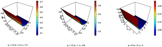
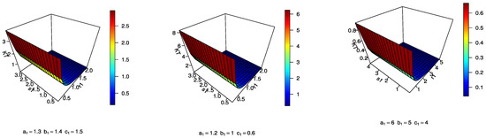
Figure 2. Coefficients of skewness and kurtosis for EKW distribution.

In the next section, we discuss a strategy of estimating parameters for the EKG model under the Bayesian paradigm using independent gamma priors.

5.1. Bayesian Estimation Using Gamma Priors for the Finite Mixture of Exponentiated Kumaraswamy-G Family

In this section, we consider the Bayes estimates of the model parameters that are obtained under the assumption that the component random variables for the random vector $\mathsf{\Phi }=[a_{j,}{b}_{j,}{c}_j,s_j,r_j,p,q,], for j=1, 2,$ have independent gamma priors with hyper parameters $a_k \mathrm{and} {Ø}_k , k=1,2,3,4,5,6,7$, which is given by

$$f\left(\mathsf{\Phi };a,Ø\right)=\frac{{Ø}_k{}^{a_k}}{\mathsf{\Gamma }{a}_k}{\mathsf{\Phi }}^{a_k-1}{e}^{-{Ø}_k\mathsf{\Phi }},\mathsf{\Phi }>0,$$

(8)

By multiplying Equation (6) with the joint posterior density of the vector $\mathsf{\Phi }$, given the data, we can obtain the following:

$$\begin{array}{l}\pi \left(\mathsf{\Phi }|\underset{\_}{x}\right)\propto L\left(\mathrm{x}|\mathsf{\Phi }\right)f\left(\mathsf{\Phi };a_k,{Ø}_k\right)\\ \hspace{0.17em}\hspace{0.17em}\hspace{0.17em}\hspace{0.17em}\hspace{0.17em}\hspace{0.17em}\propto {\displaystyle {\displaystyle \prod }_{i=1}^m}[a_1{b}_1{c}_{1}pg\left(X_{i:m:n}\right)G^{a_{1-1}}\left(X_{i:m:n}\right)\\ \hspace{0.17em}\hspace{0.17em}\hspace{0.17em}\hspace{0.17em}\hspace{0.17em}\hspace{0.17em}{\left[1-G^{a_{1-1}}\left(X_{i:m:n}\right)\right]}^{b_1-1}{\left\{{\left[1-G^{a_{1-1}}\left(X_{i:m:n}\right)\right]}^{b_1-1}\right\}}^{c_1-1}{\left[1-\left[{\left[1-G^{a_{1-1}}\left(X_{i:m:n}\right)\right]}^{b_1-1}\right]{\}}^{c_1}\right]}^{R_i}\\ \hspace{0.17em}\hspace{0.17em}\hspace{0.17em}\hspace{0.17em}\hspace{0.17em}\hspace{0.17em}+q{a}_2{b}_2{c}_{2}pg\left(X_{i:m:n}\right)G^{a_{2-1}}\left(X_{i:m:n}\right){\left[1-G^{a_{2-1}}\left(X_{i:m:n}\right)\right]}^{b_2-1}{\left[{\left[1-G^{a_{2-1}}\left(X_{i:m:n}\right)\right]}^{b_2-1}\right]}^{c_2-1}\\ \hspace{0.17em}\hspace{0.17em}\hspace{0.17em}\hspace{0.17em}\hspace{0.17em}\hspace{0.17em}{\left[1-{\left[{\left[1-G^{a_{2-1}}\left(X_{i:m:n}\right)\right]}^{b_2-1}\right]}^{c_2}\right]}^{R_i}]\frac{{Ø}_k{}^{a_k}}{\mathsf{\Gamma }{a}_k}{\mathsf{\Phi }}^{a_k-1}{e}^{-{Ø}_k\mathsf{\Phi }},\mathrm{I}\left(\mathsf{\Phi }>0\right).\end{array}$$

(9)

Marginal posterior distributions of $\mathsf{\Phi }$ can be obtained by integrating out the nuisance parameters. Next, we consider the loss function that will be used to derive the estimators from the marginal posterior distributions.

5.2. Bayes Estimation of the Vector of Parameters and Evaluation of Posterior Risk under Different Loss Functions

This section spotlights the derivation of the Bayes estimator (BE) under different loss functions and their respective posterior risks (PR). For a detailed study on different loss error functions, one can refer to [10]. The Bayes estimators are evaluated using the squared error loss function (SELF), weighted squared error loss function (WSELF), precautionary loss function (PLF), modified (quadratic) squared error loss function (M/Q SELF), logarithmic loss function (LLF), entropy loss function (ELF), and K-Loss function. The K-loss function proposed by [11] is well fitted for a measure of inaccuracy for an estimator of a scale parameter of a distribution defined by $R^{+}=\left(0,\infty \right);$ this loss function is called the K-loss function (KLF). Table 1 shows the Bayes estimators and the associated posterior risks under each specific loss functions considered in this paper.

Table 1. Bayes estimator and posterior risk under different loss functions.

Loss Function	Bayes Estimator (BE)	Posterior Risk (PR)
$L_1=SEL={\left(\mathsf{\Phi }-\hat{\mathsf{\Phi }}\right)}^2$	$E\left(\mathsf{\Phi }|X\right)$	$V\left(\mathsf{\Phi }|X\right)$
$L_2=WSEL=\frac{{\left(\mathsf{\Phi }-\hat{\mathsf{\Phi }}\right)}^2}{\mathsf{\Phi }}$	${\left[E\left({\mathsf{\Phi }}^{-1}|X\right)\right]}^{-1}$	$E\left(\mathsf{\Phi }|X\right)-{\left[E\left({\mathsf{\Phi }}^{-1}|X\right)\right]}^{-1}$
$L_3=\frac{Q}{M}SEL={\left(1-\frac{\hat{\mathsf{\Phi }}}{\mathsf{\Phi }}\right)}^2$	$\frac{E\left({\mathsf{\Phi }}^{-1}|X\right)}{E\left({\mathsf{\Phi }}^{-2}|X\right)}$	$1-\frac{E{\left({\mathsf{\Phi }}^{-1}|X\right)}^2}{E\left({\mathsf{\Phi }}^{-2}|X\right)}$
$L_4=PL=\frac{{\left(\mathsf{\Phi }-\hat{\mathsf{\Phi }}\right)}^2}{\hat{\mathsf{\Phi }}}$	$\sqrt{E\left({\mathsf{\Phi }}^2|X\right)}$	$2\left[\sqrt{E\left({\mathsf{\Phi }}^2|X\right)}-E\left(\mathsf{\Phi }|X\right)\right]$
$L_5=LL={\left(log\mathsf{\Phi }-log\hat{\mathsf{\Phi }}\right)}^2$	$exp\left[E\left(log\mathsf{\Phi }|X\right)\right]$	$V\left(log\mathsf{\Phi }|X\right)$
$L_6=EL=\left(\frac{\hat{\mathsf{\Phi }}}{\mathsf{\Phi }}-log\frac{\mathsf{\Phi }}{\hat{\mathsf{\Phi }}}-1\right)$	${\left[E\left({\mathsf{\Phi }}^{-1}|X\right)\right]}^{-1}$	$E\left(log\mathsf{\Phi }|X\right)-logE\left({\mathsf{\Phi }}^{-1}|X\right)$
$L_7=KL={\left(\sqrt{\frac{\hat{\mathsf{\Phi }}}{\mathsf{\Phi }}}-\sqrt{\frac{\mathsf{\Phi }}{\hat{\mathsf{\Phi }}}}\right)}^2$	$\sqrt{\frac{E\left(\mathsf{\Phi }|X\right)}{E\left({\mathsf{\Phi }}^{-1}|X\right)}}$	$2\left[E\left(\mathsf{\Phi }|X\right)E\left({\mathsf{\Phi }}^{-1}|X\right)-1\right]$

Next, we derive the Bayes estimators of the model parameters under different loss functions. They were originally used in estimation problems when the unbiased estimator of $\mathsf{\Phi }$ was being considered. Another reason for its popularity is due to its relationship to the least squares theory. The SEL function makes the computations simpler. Under the SEL, WSEL, $\frac{Q}{M}SEL$, PL, LL, EL and KL functions in Table 1, the Bayesian estimation for the random vector $\mathsf{\Phi }=\left(a_j,b_j,c_j,s_j,r_j,p,q\right),$ for $j=1,2$, and under various loss functions, it can be obtained as follows.

$${\hat{\mathsf{\Phi }}}_{SEL}=E\left(\mathsf{\Phi }|\underset{\_}{x}\right)={{\displaystyle \int }}_{\mathsf{\Phi }}^{}{\left(\mathsf{\Phi }-\hat{\mathsf{\Phi }}\right)}^2\pi \left(\mathsf{\Phi }|\underset{\_}{x}\right)d\mathsf{\Phi }.$$

$${\hat{\mathsf{\Phi }}}_{WSEL}=E\left(\mathsf{\Phi }|\underset{\_}{x}\right)=\underset{\mathsf{\Phi }}{\overset{}{{\displaystyle \int }}}\frac{{\left(\mathsf{\Phi }-\hat{\mathsf{\Phi }}\right)}^2}{\mathsf{\Phi }}\pi \left(\mathsf{\Phi }|\underset{\_}{x}\right)d\mathsf{\Phi }.$$

$${\hat{\mathsf{\Phi }}}_{\frac{Q}{M}SEL}=E\left(\mathsf{\Phi }|\underset{\_}{x}\right)={{\displaystyle \int }}_{\mathsf{\Phi }}^{}{\left(1-\frac{\hat{\mathsf{\Phi }}}{\mathsf{\Phi }}\right)}^2\pi \left(\mathsf{\Phi }|\underset{\_}{x}\right)d\mathsf{\Phi }.$$

$${\hat{\mathsf{\Phi }}}_{PL}=E\left(\mathsf{\Phi }|\underset{\_}{x}\right)={{\displaystyle \int }}_{\mathsf{\Phi }}^{}\frac{{\left(\mathsf{\Phi }-\hat{\mathsf{\Phi }}\right)}^2}{\hat{\mathsf{\Phi }}}\pi \left(\mathsf{\Phi }|\underset{\_}{x}\right)d\mathsf{\Phi }.$$

$${\hat{\mathsf{\Phi }}}_{LL}=E\left(\mathsf{\Phi }|\underset{\_}{x}\right)={{\displaystyle \int }}_{\mathsf{\Phi }}^{}{\left(log\mathsf{\Phi }-log\hat{\mathsf{\Phi }}\right)}^2\pi \left(\mathsf{\Phi }|\underset{\_}{x}\right)d\mathsf{\Phi }.$$

$${\hat{\mathsf{\Phi }}}_{KL}=E\left(\mathsf{\Phi }|\underset{\_}{x}\right)={{\displaystyle \int }}_{\mathsf{\Phi }}^{}{\left(\sqrt{\frac{\hat{\mathsf{\Phi }}}{\mathsf{\Phi }}}-\sqrt{\frac{\mathsf{\Phi }}{\hat{\mathsf{\Phi }}}}\right)}^2\pi \left(\mathsf{\Phi }|\underset{\_}{x}\right)d\mathsf{\Phi }.$$

(10)

It is evident that each of the integrals in the above section have no closed form for the resulting joint posterior distribution as given in Equation (9). Therefore, they need to be solved analytically. Consequently, the MCMC technique is proposed to generate samples from the posterior distributions and then the Bayes estimates of the parameter vector $\mathsf{\Phi }$ are computed under progressively type II censored samples. Next, we provide the general form of the Bayesian credible intervals.

5.3. Credible Intervals

In this subsection, asymmetric $100\left(1-\tau \right)\%$ two-sided Bayes probability interval estimates of the parameter vector $\mathsf{\Phi }$, denoted by $\left[{\mathrm{L}}_{\mathsf{\Phi }},{\mathrm{U}}_{\mathsf{\Phi }}\right]$, are obtained by solving the following expression:

$$p\left[\mathrm{L}\left(\underset{\_}{\mathrm{t}}\right)<\mathsf{\Phi }<\mathrm{U}\left(\underset{\_}{\mathrm{t}}\right)\right]={{\displaystyle \int }}_{\mathrm{L}\left(\underset{\_}{\mathrm{t}}\right)}^{\mathrm{U}\left(\underset{\_}{\mathrm{t}}\right)}\mathsf{\pi }\left(\mathsf{\theta },\mathsf{\beta },\mathsf{\lambda }|\underset{\_}{\mathrm{t}}\right)\mathrm{d}\mathsf{\Phi }=1-\mathsf{\tau }.$$

(11)

Since it is difficult to find the interval ${\mathrm{L}}_{\mathsf{\Phi }}$ and ${\mathrm{U}}_{\mathsf{\Phi }}$ analytically, we apply suitable numerical techniques to solve Equation (11).

6. Bayesian Estimation of the Exponentiated Kumaraswamy Weibull Distribution

G is assumed to be the Weibull distribution with pdf and cdf, which are given by

$$g\left(x\right)=\frac{r}{s}{\left(\frac{x}{s}\right)}^{r-1}exp\left[-{\left(\frac{x}{s}\right)}^r\right],$$

where r is the shape parameter $(r>0),$ and s is the scale parameter $\left(s>0\right)$ and

$$G\left(x\right)=\left(1-exp\left[-{\left(\frac{x}{s}\right)}^r\right]\right),x>0.$$

The joint posterior density for the parameter vector $\mathsf{\Phi }$, given the data, becomes the following:

$$\begin{array}{l}\pi \left(\mathsf{\Phi }|\underset{\_}{x}\right)\propto L\left(\mathrm{x}|\mathsf{\Phi }\right)f\left(\mathsf{\Phi };a_k,{Ø}_k\right)\\ \hspace{0.17em}\hspace{0.17em}\hspace{0.17em}\hspace{0.17em}\hspace{0.17em}\hspace{0.17em}\hspace{0.17em}\hspace{0.17em}\hspace{0.17em}\hspace{0.17em}\propto {\displaystyle {\displaystyle \prod }_{i=1}^m}[a_1{b}_1{c}_{1}p\frac{r_1}{s_1}{\left(\frac{x}{s_1}\right)}^{r_1-1}exp\left[-{\left(\frac{x}{s_1}\right)}^{r_1}\right]{\left[1-exp\left[-{\left(\frac{x}{s_1}\right)}^{r_1}\right]\right]}^{a_{1-1}}\\ \hspace{0.17em}\hspace{0.17em}\hspace{0.17em}\hspace{0.17em}\hspace{0.17em}\hspace{0.17em}\hspace{0.17em}\hspace{0.17em}\hspace{0.17em}\hspace{0.17em}{\left[1-{\left[1-exp\left[-{\left(\frac{x}{s_1}\right)}^{r_1}\right]\right]}^{a_{1-1}}\right]}^{b_1-1}]{\left\{{\left[1-{\left[1-exp\left[-{\left(\frac{x}{s_1}\right)}^{r_1}\right]\right]}^{a_{1-1}}\right]}^{b_1-1}\right\}}^{c_1-1}\\ \hspace{0.17em}\hspace{0.17em}\hspace{0.17em}\hspace{0.17em}\hspace{0.17em}\hspace{0.17em}\hspace{0.17em}\hspace{0.17em}\hspace{0.17em}\hspace{0.17em}{\left[1-{\left[{\left[1-{\left[1-exp\left[-{\left(\frac{x}{s_1}\right)}^{r_1}\right]\right]}^{a_{1-1}}\right]}^{b_1-1}\right]}^{c_1}\right]}^{R_i}\\ \hspace{0.17em}\hspace{0.17em}\hspace{0.17em}\hspace{0.17em}\hspace{0.17em}\hspace{0.17em}\hspace{0.17em}\hspace{0.17em}\hspace{0.17em}\hspace{0.17em}+q{a}_2{b}_2{c}_2\frac{r_2}{s_2}{\left(\frac{x}{s_2}\right)}^{r_2-1}exp\left[-{\left(\frac{x}{s_2}\right)}^{r_2}\right]{\left[1-exp\left[-{\left(\frac{x}{s_2}\right)}^{r_2}\right]\right]}^{a_{2-1}}\\ \hspace{0.17em}\hspace{0.17em}\hspace{0.17em}\hspace{0.17em}\hspace{0.17em}\hspace{0.17em}\hspace{0.17em}\hspace{0.17em}\hspace{0.17em}\hspace{0.17em}{\left[1-{\left[1-exp\left[-{\left(\frac{x}{s_2}\right)}^{r_2}\right]\right]}^{a_{2-1}}\right]}^{b_2-1}{\left[{\left[1-{\left[1-exp\left[-{\left(\frac{x}{s_2}\right)}^{r_2}\right]\right]}^{a_{2-1}}\right]}^{b_2-1}\right]}^{c_2-1}\\ \hspace{0.17em}\hspace{0.17em}\hspace{0.17em}\hspace{0.17em}\hspace{0.17em}\hspace{0.17em}\hspace{0.17em}\hspace{0.17em}\hspace{0.17em}\hspace{0.17em}{\left[1-{\left[{\left[1-{\left[1-exp\left[-{\left(\frac{x}{s_2}\right)}^{r_2}\right]\right]}^{a_{2-1}}\right]}^{b_2-1}\right]}^{c_2}\right]}^{R_i}\frac{{Ø}_k{}^{a_k}}{\mathsf{\Gamma }{a}_k}{\mathsf{\Phi }}^{a_k-1}{e}^{-{Ø}_k\mathsf{\Phi }},\mathrm{I}\left(\mathsf{\Phi }>0\right)\end{array}$$

(12)

Marginal distributions of the parameter vector $\mathsf{\Phi }$ can be obtained by integrating the nuisance parameters. Next, we consider the loss function that will be used to derive the estimators from the marginal posterior distributions.

7. Simulation Study

In this section, we evaluate the performance of the maximum likelihood and the Bayesian estimation methods to estimate the parameters using Monte Carlo simulations. We conduct the simulations using the (Maxlik) package in R software, as shown in [12]. The values of the biases, and the relative mean square errors (RMSEs) in the results indicate that the maximum likelihood and the Bayesian estimation methods performs quite well to estimate the model parameters.

Simulation Study for MEKW

In this subsection, we evaluate the performance of the maximum likelihood method and Bayesian estimation method to estimate the parameters for the MEKW model using Monte Carlo simulations. Based on progressively type II censored samples selected from the MEKW pdf in Equation (3), a total of eight parameter combinations, and assuming the sample sizes n = 25, 50, censored at 60% and 80% of the sample size, are considered. The process is repeated 1000 times and the biases (estimate–actual), RMSEs and length of confidence intervals (CI) of the estimates are reported in Table 2, Table 3, Table 4, Table 5, Table 6 and Table 7. In computing the length of CI, we obtain length asymptotic CI (LACI) for the likelihood estimators, and also obtain the length credible CI (LCCI) for the Bayesian estimators. In addition, we compared the performance of the estimation by considering the following schemes.

Table 2. Bias, RMSE and length of CI for the MLE and Bayesian estimates of the parameters are presented for different sample sizes: Scheme 1 (complete sample), Case 1.

		MLE			Bayesian
n		Bias	RMSE	LACI	Bias	RMSE	LCCI
25	a1	0.1363	0.7467	2.8809	0.0743	0.2569	0.9628
	b1	−0.2161	0.7758	2.9236	0.1091	0.2275	0.7848
	c1	0.1374	0.9482	3.6814	0.0941	0.2920	0.9927
	r1	0.6883	1.2519	4.1030	0.1441	0.2783	0.8962
	s1	−0.1083	0.3819	1.4369	0.0243	0.1426	0.5350
	a2	0.2119	0.8836	3.3659	0.1080	0.2499	0.8166
	b2	−0.2985	0.8408	3.0842	0.1432	0.3119	1.0558
	c2	0.2908	1.0364	3.9034	0.0380	0.2224	0.8259
	r2	0.7734	1.4002	4.5801	0.1438	0.2855	0.9685
	s2	−0.2023	0.5034	1.8088	0.0052	0.0335	0.1289
	p	−0.0112	0.0952	0.3710	−0.0342	0.0885	0.3028
50	a1	0.0325	0.6253	2.4502	0.0364	0.1648	0.6325
	b1	−0.1865	0.6440	2.4185	0.0602	0.1333	0.4764
	c1	0.0006	0.7457	2.9259	0.0262	0.1634	0.6277
	r1	0.5867	0.9923	3.1401	0.1102	0.1835	0.5522
	s1	−0.0360	0.3025	1.1784	0.0103	0.0898	0.3480
	a2	0.1064	0.7523	2.9225	0.0364	0.1389	0.5130
	b2	−0.1927	0.6604	2.4784	0.1101	0.2216	0.7209
	c2	0.1501	0.8913	3.4475	0.0396	0.1470	0.5468
	r2	0.6011	1.0677	3.4625	0.0978	0.1756	0.5552
	s2	−0.1098	0.4171	1.5790	0.0000	0.0219	0.0854
	p	−0.0012	0.0648	0.2540	−0.0146	0.0622	0.2353
100	a1	−0.0776	0.5013	1.9434	0.0156	0.1205	0.4462
	b1	−0.1608	0.5400	2.0228	0.0506	0.1193	0.4208
	c1	−0.1454	0.5745	2.1809	0.0136	0.1412	0.5552
	r1	0.6321	0.9161	2.6022	0.1030	0.1609	0.4740
	s1	0.0369	0.2611	1.0143	−0.0010	0.0701	0.2702
	a2	0.0565	0.6470	2.5289	0.0162	0.1004	0.3790
	b2	−0.1245	0.6024	2.3128	0.0673	0.1583	0.5709
	c2	0.0053	0.7704	3.0230	0.0203	0.1138	0.4199
	r2	0.5095	0.9132	2.9741	0.0713	0.1396	0.4697
	s2	−0.0214	0.3687	1.4443	−0.0005	0.0179	0.0671
	p	0.0019	0.0521	0.2043	−0.0050	0.0497	0.1896

Table 3. Bias, RMSE and length of CI for the MLE and Bayesian estimates of the parameters are presented for different schemes: Case 1 and n = 25.

			MLE			Bayesian
Scheme	n, m		Bias	RMSE	LACI	Bias	RMSE	LCCI
2	25, 15	a1	0.2086	0.6935	2.5950	0.1157	0.2775	0.9395
		b1	−0.3516	0.7858	2.7576	0.0911	0.2282	0.7983
		c1	0.1511	0.7569	2.9101	0.0765	0.2676	0.9211
		r1	0.5921	1.1801	4.0056	0.1478	0.3511	1.1950
		s1	−0.2418	0.4328	1.4085	0.0366	0.2240	0.8323
		a2	0.3463	0.9475	3.4605	0.0217	0.2295	0.8224
		b2	−0.4146	0.9381	3.3021	0.2170	0.4221	1.4613
		c2	0.2505	0.8901	3.3515	0.0471	0.2519	0.9327
		r2	1.1189	1.5792	4.3727	0.1465	0.2942	0.9666
		s2	−0.4516	0.6420	1.7906	−0.0091	0.0436	0.1606
		p	0.0232	0.2115	0.8248	−0.0054	0.1803	0.5545
	25, 20	a1	0.1707	0.6897	2.5622	0.0455	0.1439	0.5135
		b1	−0.3438	0.7705	2.7060	0.0500	0.1341	0.4665
		c1	0.0316	0.7494	2.9038	0.0436	0.1566	0.5762
		r1	0.6538	1.0314	3.3474	0.0571	0.2067	0.7663
		s1	−0.1799	0.4067	1.3144	0.0404	0.1491	0.5154
		a2	0.2747	0.8731	3.2521	0.0371	0.1507	0.5460
		b2	−0.3155	0.8002	2.8854	0.1040	0.2557	0.8661
		c2	0.2094	0.8093	3.0556	0.0354	0.1428	0.5314
		r2	0.9609	1.2634	3.0120	0.0999	0.1988	0.6814
		s2	−0.2952	0.5144	1.6531	−0.0030	0.0250	0.0908
		p	0.0099	0.1339	0.5238	−0.0169	0.1143	0.4068
3	25, 15	a1	0.1161	0.7157	2.7713	0.0909	0.2582	0.9175
		b1	−0.3936	0.7869	2.6737	0.0994	0.2208	0.7204
		c1	0.1617	0.8577	3.3051	0.0683	0.2632	0.9451
		r1	0.6209	1.2826	4.4038	0.1023	0.2885	0.9627
		s1	−0.1745	0.4339	1.5587	0.0754	0.1732	0.6193
		a2	0.2977	0.8905	3.2933	0.0859	0.2325	0.8070
		b2	−0.3494	0.8102	2.8682	0.1131	0.3168	1.0870
		c2	0.3593	0.9570	3.4806	0.0930	0.2529	0.8532
		r2	0.7486	1.2881	4.1132	0.1310	0.2876	0.9885
		s2	−0.2523	0.5078	1.7293	0.0091	0.0347	0.1240
		p	−0.0110	0.2158	0.8458	−0.0355	0.1884	0.5606
	25, 20	a1	0.1607	0.7128	2.7250	0.0563	0.1489	0.5512
		b1	−0.2165	0.7084	2.5194	0.0502	0.1247	0.4392
		c1	0.1249	0.8100	3.0788	0.0470	0.1634	0.6065
		r1	0.5943	1.0322	3.6334	0.0650	0.1916	0.6970
		s1	−0.1554	0.4023	1.4562	0.0235	0.1069	0.4019
		a2	0.1888	0.8684	3.2622	0.0552	0.1365	0.4698
		b2	−0.2937	0.8115	2.6968	0.0614	0.1984	0.6992
		c2	0.2993	0.8063	3.0035	0.0473	0.1400	0.5285
		r2	0.5807	1.0457	4.0757	0.0732	0.1829	0.6418
		s2	−0.1663	0.5084	1.4885	0.0048	0.0200	0.0761
		p	−0.0107	0.1419	0.5554	−0.0354	0.1267	0.4211

Table 4. Bias, RMSE and length of CI for the MLE and Bayesian estimates of the parameters are presented for different schemes: Case 1 and n = 50.

			MLE			Bayesian
Scheme	n, m		Bias	RMSE	LACI	Bias	RMSE	LCCI
2	50, 30	a1	0.1740	0.6464	2.4428	0.0985	0.2686	0.9424
		b1	−0.2839	0.6850	2.4461	0.1049	0.2627	0.9051
		c1	0.0535	0.6684	2.6143	0.0815	0.2862	0.9613
		r1	0.4536	1.0329	3.6413	0.1323	0.3722	1.2898
		s1	−0.1768	0.3914	1.3701	0.0462	0.2367	0.8292
		a2	0.1538	0.7803	3.0018	−0.0047	0.2490	0.9586
		b2	−0.3140	0.7485	2.6661	0.3206	0.5488	1.6380
		c2	0.0664	0.7585	2.9649	0.0245	0.2544	0.9684
		r2	1.1236	1.6130	4.5412	0.2103	0.3669	1.1379
		s2	−0.3536	0.5499	1.6526	−0.0264	0.0637	0.2052
		p	0.0273	0.1937	0.7527	0.0109	0.1774	0.5251
	50, 40	a1	0.1385	0.6058	2.3526	0.0378	0.1515	0.5607
		b1	−0.3216	0.6863	2.3792	0.0357	0.1402	0.5168
		c1	0.0496	0.5807	2.5146	0.0318	0.1757	0.6541
		r1	0.4528	0.9119	3.5998	0.0671	0.2231	0.7929
		s1	−0.1435	0.3782	1.3732	0.0488	0.1514	0.5324
		a2	0.1669	0.7759	2.9731	0.0134	0.1514	0.5693
		b2	−0.1764	0.7496	2.5859	0.1789	0.3302	0.9973
		c2	−0.0199	0.7398	2.9020	0.0129	0.1412	0.5300
		r2	1.0421	1.5571	4.5399	0.1420	0.2564	0.8151
		s2	−0.2003	0.4252	1.4718	−0.0121	0.0342	0.1166
		p	0.0261	0.1170	0.4475	0.0095	0.1047	0.3537
3	50, 30	a1	0.1031	0.6498	2.5174	0.0779	0.2654	0.9538
		b1	−0.2174	0.6665	2.4724	0.0968	0.2433	0.8425
		c1	0.1599	0.7887	3.0306	0.0804	0.3027	1.0356
		r1	0.3891	0.9908	3.5757	0.0807	0.2552	0.9065
		s1	−0.1131	0.3722	1.3915	0.0546	0.1587	0.5932
		a2	0.2047	0.7134	2.6817	0.0921	0.2352	0.7769
		b2	−0.1824	0.6974	2.6414	0.0814	0.2837	0.9804
		c2	0.2089	0.8528	3.2443	0.0572	0.2373	0.8509
		r2	0.4022	0.9146	3.2231	0.1108	0.2715	0.9205
		s2	−0.1485	0.4358	1.6076	0.0124	0.0368	0.1380
		p	−0.0058	0.2060	0.8079	−0.0190	0.1904	0.5459
	50, 40	a1	0.1919	0.6064	2.4934	0.0457	0.1469	0.5373
		b1	−0.1360	0.6266	2.4002	0.0501	0.1353	0.4797
		c1	0.2024	0.6306	2.9215	0.0371	0.1646	0.6183
		r1	0.2577	0.8736	3.2753	0.0444	0.1767	0.6505
		s1	−0.1101	0.3609	1.3485	0.0333	0.0997	0.3671
		a2	0.1838	0.7048	2.5844	0.0389	0.1382	0.5167
		b2	−0.1898	0.6913	2.6081	0.0503	0.1826	0.6657
		c2	0.2209	0.8492	3.1514	0.0355	0.1405	0.5139
		r2	0.4817	0.9032	3.1583	0.0666	0.1764	0.6511
		s2	−0.1363	0.4060	1.5724	0.0040	0.0233	0.0878
		p	−0.0106	0.1194	0.4667	−0.0238	0.1120	0.3631

Table 5. Bias, RMSE and length of CI for the MLE and Bayesian estimates of the parameters are presented for different sample sizes: Scheme 1 (complete sample), Case 2.

		MLE			Bayesian
n		Bias	RMSE	LACI	Bias	RMSE	LCCI
25	a1	0.4950	1.2585	5.9078	0.1046	0.2725	0.9632
	b1	0.0025	0.0974	0.3819	0.0691	0.0811	0.3175
	c1	0.3392	1.2556	4.7436	0.0663	0.1757	0.6258
	r1	0.1166	0.2492	0.8640	−0.0189	0.1458	0.5568
	s1	0.1338	0.4568	1.7138	0.1819	0.2823	0.8286
	a2	0.0850	1.9085	7.4814	0.0398	0.1079	0.3711
	b2	0.0461	0.1245	0.4540	0.0312	0.0675	0.2063
	c2	0.2599	0.5643	1.9656	0.0475	0.2313	0.7513
	r2	0.0984	0.3444	1.2950	−0.0534	0.1993	0.7545
	s2	−0.0048	0.3695	1.4497	0.0216	0.0382	0.1283
	p	−0.0035	0.0920	0.3607	−0.0116	0.0816	0.3071
50	a1	0.2532	1.0781	4.9156	0.0615	0.1727	0.6082
	b1	0.0039	0.0774	0.3032	0.0425	0.0778	0.2230
	c1	0.3267	1.0900	4.0806	0.0339	0.1189	0.4407
	r1	0.0774	0.1588	0.5440	−0.0128	0.1009	0.3987
	s1	0.1067	0.4314	1.6401	0.0985	0.1755	0.5609
	a2	−0.1625	1.4809	5.7759	0.0299	0.0781	0.2910
	b2	0.0457	0.1183	0.4281	0.0296	0.0515	0.1509
	c2	0.2415	0.4634	1.8299	0.0410	0.1641	0.5968
	r2	0.0369	0.2309	0.8944	−0.0655	0.1306	0.4482
	s2	0.0314	0.3073	1.4569	0.0157	0.0265	0.0823
	p	−0.0036	0.0692	0.2712	−0.0094	0.0648	0.2451
100	a1	0.1000	0.9519	3.7145	0.0397	0.1558	0.5863
	b1	0.0054	0.0522	0.2037	0.0249	0.0539	0.1661
	c1	0.2833	0.7983	2.9286	0.0349	0.1158	0.4385
	r1	0.0534	0.1129	0.3903	0.0063	0.0776	0.3142
	s1	0.0688	0.3142	1.2030	0.0658	0.1410	0.4920
	a2	−0.1731	1.1550	4.4811	0.0199	0.0732	0.2684
	b2	0.0396	0.0985	0.3541	0.0233	0.0381	0.1088
	c2	0.1359	0.3042	1.0677	0.0174	0.1019	0.3844
	r2	0.0006	0.1304	0.5117	−0.0566	0.0978	0.3237
	s2	0.0363	0.2320	1.2465	0.0114	0.0254	0.0740
	p	−0.0014	0.0485	0.1903	−0.0031	0.0472	0.1834

Table 6. Bias, RMSE and length of CI for the MLE and Bayesian estimates of the parameters are presented for different schemes: Case 2 and n = 25.

			MLE			Bayesian
Scheme	n, m		Bias	RMSE	LACI	Bias	RMSE	LCCI
2	25, 15	a1	0.3219	1.5006	5.7511	0.0890	0.2609	0.9529
		b1	−0.0140	0.1061	0.4125	0.0409	0.1046	0.3430
		c1	0.2475	1.3018	5.0149	0.0303	0.1680	0.6187
		r1	0.3045	0.6054	2.0533	0.1003	0.2511	0.8449
		s1	0.1760	0.5871	2.1980	0.1423	0.2544	0.7830
		a2	−0.1057	2.0364	7.9800	0.0373	0.1059	0.3868
		b2	0.0533	0.2103	0.7982	0.0260	0.0679	0.2227
		c2	0.2514	0.6190	2.2198	0.0491	0.2189	0.7067
		r2	0.2421	0.5800	2.0680	−0.0026	0.2304	0.9165
		s2	0.1230	0.5706	2.1865	0.0203	0.0362	0.1182
		p	−0.0230	0.1544	0.5992	−0.0320	0.1371	0.5096
	25, 20	a1	0.4450	1.2772	4.7292	0.0502	0.1432	0.5073
		b1	−0.0071	0.1040	0.4072	0.0391	0.0990	0.3048
		c1	0.2764	1.2067	4.6092	0.0235	0.1010	0.3778
		r1	0.1954	0.4030	1.3830	0.0309	0.1768	0.6555
		s1	0.1461	0.5049	1.8965	0.0819	0.1589	0.5218
		a2	0.1944	2.0450	7.9880	0.0235	0.0627	0.2217
		b2	0.0341	0.1379	0.5242	0.0239	0.0581	0.1891
		c2	0.2256	0.6054	2.2044	0.0551	0.2044	0.7016
		r2	0.1582	0.4093	1.4811	−0.0506	0.1708	0.6461
		s2	0.0712	0.4372	1.6925	0.0127	0.0223	0.0712
		p	−0.0200	0.1178	0.4557	−0.0314	0.1056	0.3854
3	25, 15	a1	0.3756	1.5466	5.8871	0.0977	0.2491	0.8675
		b1	0.0086	0.1149	0.4497	0.0728	0.1016	0.3220
		c1	0.2402	1.1652	4.4740	0.0407	0.1576	0.6094
		r1	0.1513	0.2897	0.9695	−0.0267	0.1492	0.5809
		s1	0.2196	0.5639	2.0382	0.1517	0.2645	0.8215
		a2	0.0220	1.8220	7.1490	0.0473	0.1138	0.3973
		b2	0.0456	0.1589	0.5971	0.0289	0.0658	0.2128
		c2	0.2686	0.6084	2.1420	0.0957	0.2510	0.8332
		r2	0.2490	0.4789	1.6053	−0.0177	0.2134	0.8030
		s2	0.1015	0.4697	1.7995	0.0246	0.0406	0.1244
		p	−0.1750	0.2005	0.3840	−0.1599	0.1814	0.3204
	25, 20	a1	0.3345	1.4388	5.4909	0.0556	0.1509	0.5303
		b1	0.0026	0.1035	0.4058	0.0504	0.0942	0.2754
		c1	0.3566	1.0276	4.2807	0.0291	0.1015	0.3685
		r1	0.1413	0.2619	0.8653	−0.0160	0.1250	0.4882
		s1	0.1898	0.5521	2.0346	0.0960	0.1626	0.5275
		a2	0.2065	1.7882	5.3390	0.0242	0.0622	0.2171
		b2	0.0523	0.1422	0.5190	0.0218	0.0566	0.1773
		c2	0.3228	0.5461	2.0235	0.0667	0.2028	0.7112
		r2	0.1509	0.4165	1.5231	−0.0344	0.1565	0.5786
		s2	0.0576	0.4180	1.6247	0.0128	0.0232	0.0730
		p	−0.0859	0.1294	0.3797	−0.0773	0.1171	0.3043

Table 7. Bias, RMSE and length of CI for the MLE and Bayesian estimates of the parameters are presented for different schemes: Case 2 and n = 50.

			MLE			Bayesian
Scheme	n, m		Bias	RMSE	LACI	Bias	RMSE	LCCI
I	50, 30	a1	0.1607	1.1624	4.5175	0.0950	0.2756	0.9877
		b1	−0.0156	0.0926	0.3583	0.0425	0.1156	0.3975
		c1	0.1410	0.9550	3.7064	0.0340	0.1804	0.7061
		r1	0.3582	0.6997	2.3586	0.1390	0.3104	1.0253
		s1	0.1687	0.6128	2.3115	0.1347	0.2730	0.8936
		a2	−0.3925	1.4224	5.3648	0.0466	0.1148	0.4057
		b2	0.0444	0.1538	0.5779	0.0233	0.0643	0.2126
		c2	0.1707	0.4040	1.4368	0.0621	0.2132	0.7099
		r2	0.2614	0.6599	2.3776	0.0353	0.2589	0.9918
		s2	0.1804	0.6739	2.5479	0.0192	0.0394	0.1334
		p	−0.0440	0.2016	0.7719	−0.0479	0.1859	0.5668
	50, 40	a1	0.1322	1.0365	4.2045	0.0616	0.1823	0.6517
		b1	−0.0061	0.0903	0.3536	0.0218	0.0800	0.2685
		c1	0.1406	0.9028	3.6985	0.0214	0.1105	0.4222
		r1	0.1619	0.3606	1.2642	0.0606	0.1810	0.6664
		s1	0.1229	0.4318	1.6243	0.0673	0.1532	0.5163
		a2	−0.2044	1.3552	4.5038	0.0219	0.0698	0.2580
		b2	0.0286	0.1166	0.4435	0.0224	0.0498	0.1704
		c2	0.1682	0.3741	1.4034	0.0500	0.1703	0.5965
		r2	0.1231	0.3405	1.2457	−0.0294	0.1568	0.6370
		s2	0.0647	0.4849	1.8859	0.0107	0.0238	0.0771
		p	−0.0117	0.1050	0.4094	−0.0171	0.0996	0.3911
II	50, 30	a1	0.3428	1.2479	4.7083	0.1173	0.3037	1.1006
		b1	0.0019	0.0856	0.3357	0.0651	0.1078	0.2946
		c1	0.2610	1.0548	4.0104	0.0631	0.1839	0.6537
		r1	0.1252	0.2271	0.7435	−0.0133	0.1284	0.5061
		s1	0.1625	0.4028	1.4461	0.1708	0.2807	0.7910
		a2	−0.0189	1.2375	4.8553	0.0595	0.1238	0.4057
		b2	0.0300	0.0986	0.3684	0.0344	0.0626	0.1887
		c2	0.1687	0.3744	1.3115	0.1112	0.2300	0.7343
		r2	0.1328	0.3041	1.0733	−0.0624	0.1694	0.5980
		s2	0.0893	0.3474	1.3174	0.0302	0.0480	0.1460
		p	−0.2414	0.2501	0.2563	−0.2261	0.2345	0.2025
	50, 40	a1	0.1323	0.9504	4.6244	0.0602	0.1719	0.6060
		b1	0.0084	0.0855	0.3337	0.0488	0.0886	0.2672
		c1	0.2795	0.8144	3.8352	0.0355	0.1176	0.4267
		r1	0.0950	0.1849	0.6223	−0.0175	0.1077	0.4235
		s1	0.1539	0.3912	1.4114	0.0958	0.1742	0.5624
		a2	−0.1510	0.9435	4.5993	0.0280	0.0748	0.2571
		b2	0.0406	0.0914	0.3440	0.0239	0.0483	0.1573
		c2	0.1276	0.3428	1.2532	0.0524	0.1699	0.6015
		r2	0.1008	0.2956	1.0090	−0.0475	0.1378	0.4887
		s2	0.0880	0.3042	1.2462	0.0133	0.0258	0.0864
		p	−0.1212	0.1366	0.2472	−0.1148	0.1298	0.1923

Scheme 1.

$R_{kı}=0, ı=1,\dots , n_k-m_k$

Scheme 2.

$R_{kı}=\{\begin{array}{c}{n}_k-m_k, ı=1\\ 0, ı=2,\dots ,m_k \end{array}$

Scheme 3.

$R_{kı}=\{\begin{array}{c}{n}_k-m_k, ı=m_k\\ 0, ı=1,\dots ,m_{k-1} \end{array}$

MLE, average bias Abs(Bias) and the RMSE for the MLE of the parameters are presented for different sample sizes and different sampling schemes

For Case 1, the selected initial values are as follows: a1 = 1.4, b1 = 1.5, c1 = 1.35, r1 = 1.7, s1 = 1.2, a2 = 1.4, b2 = 1.5, c2 = 1.35, r2 = 1.5, s2 = 1.3; p = 0.7.

For Case 2, the initial values are a1 = 1.8, b1 = 0.2, c1 = 3.5, r1 = 1.2, s1 = 1.5, a2 = 4, b2 = 0.1, c2 = 0.65, r2 = 1.5, s2 = 1.3, p = 0.6.

8. Application on Bladder Cancer Data

In this section, we provide a real data analysis to illustrate some practical applications of the proposed distributions. The data are from [13], which correspond to the remission times (in months) of a random sample of n = 128 bladder cancer patients. These data are given as follows:

0.08, 2.09, 3.48, 4.87, 6.94, 8.66, 13.11, 23.63, 0.20, 2.23, 3.52, 4.98, 6.97, 9.02, 13.29, 0.40, 2.26, 3.57, 5.06, 7.09, 9.22, 13.80, 25.74, 0.50, 2.46, 3.64, 5.09, 7.26, 9.47, 14.24, 25.82, 0.51, 2.54, 3.70, 5.17, 7.28, 9.74, 14.76, 26.31, 0.81, 2.62, 3.82, 5.32, 7.32, 10.06, 14.77, 32.15, 2.64, 3.88, 5.32, 7.39, 10.34, 14.83, 34.26, 0.90, 2.69, 4.18, 5.34, 7.59, 10.66, 15.96, 36.66, 1.05, 2.69, 4.23, 5.41, 7.62, 10.75, 16.62, 43.01, 1.19, 2.75, 4.26, 5.41, 7.63, 17.12, 46.12, 1.26, 2.83, 4.33, 5.49, 7.66, 11.25, 17.14, 79.05, 1.35, 2.87, 5.62, 7.87, 11.64, 17.36, 1.40, 3.02, 4.34, 5.71, 7.93, 11.79, 18.10, 1.46, 4.40, 5.85, 8.26, 11.98, 19.13, 1.76, 3.25, 4.50, 6.25, 8.37, 12.02, 2.02, 3.31, 4.51, 6.54, 8.53, 12.03, 20.28, 2.02, 3.36, 6.76, 12.07, 21.73, 2.07, 3.36, 6.93, 8.65, 12.63, 22.69.

Before proceeding further, we fitted the mixture EKW distribution to the complete data set. Table 8 reports the ML and Bayesian estimates for the parameters for the complete bladder cancer data. Figure 3 represents the overall fit of EKW for these data.

Table 8. ML estimates of the EKW parameters with the corresponding bladder data.

	a	b	c	r	s	KSD	PVKS	CVM	AD
Estimates	3.6537	3.1179	1.1311	0.4578	5.2873	0.0443	0.9629	0.0408	0.2700

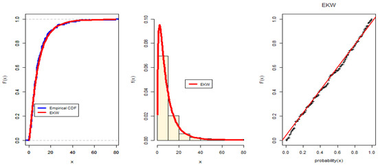
Figure 3. ML estimates of the EKW parameters for the complete bladder cancer data.

The validity of the fitted model is assessed by computing the Kolmogorov–Smirnov distance (KSD) statistics with p-Value KS (PVKS) in Table 8. In addition, we plotted the fitted cdf and the empirical cdf, as shown in Figure 3. This was conducted by replacing the parameters with their ML (in red) estimates, as shown in Figure 3. The KSD statistics for ML are 0.0443 and the corresponding p-value is 0.9629. Therefore, the KS test, along with Figure 3, indicate that the EKW distribution provides the best fit for this data set.

Next, we fitted the MEKW distribution to the complete data set. Table 9 reports the ML and Bayesian estimates for the parameters for the complete bladder cancer data.

Table 9. ML estimates of the MEKW parameters for the complete sample of the bladder data.

	MLE				Bayesian
	Estimates	SE	Lower	Upper	Estimates	SE	Lower	Upper
a1	8.2459	0.0171	8.2125	8.2794	8.3297	0.0075	8.2310	8.2601
b1	0.1491	0.0123	0.1250	0.1733	0.1866	0.0008	0.1477	0.1506
c1	27.6825	7.5314	12.9208	42.4441	27.2578	0.1975	27.5327	27.8240
r1	1.1925	0.0015	1.1896	1.1954	1.1456	0.0015	1.1800	1.1984
s1	4.4770	0.0014	4.4742	4.4798	4.3029	0.0003	4.4620	4.4911
a2	12.2492	0.0079	12.2337	12.2648	12.2200	0.0075	12.2343	12.2634
b2	0.1526	0.0126	0.1279	0.1773	0.2207	0.0008	0.1511	0.1540
c2	22.6763	5.8063	11.2960	34.0567	22.6720	0.0754	22.5266	22.8179
r2	1.2810	0.0024	1.2763	1.2858	0.3040	0.0014	1.2661	1.2952
s2	5.6261	0.0026	5.6210	5.6313	0.1922	0.0025	5.6115	5.6406
p	0.5004	0.0347	0.4325	0.5684	0.6039	0.0075	0.4858	0.5149

In Figure 4 and Figure 5, we provide the trace plots of the MCMC results, showing the MCMC procedure converges. Figure 6 and Figure 7 show the MCMC density and HDI intervals for the results of the Bayesian estimation of the MEKW model for the complete sample. Therefore, we will use the estimate for the mixing parameter $\widehat{\rho }=0.5004$ in computing the ML and Bayesian estimates for other parameters when using complete samples.

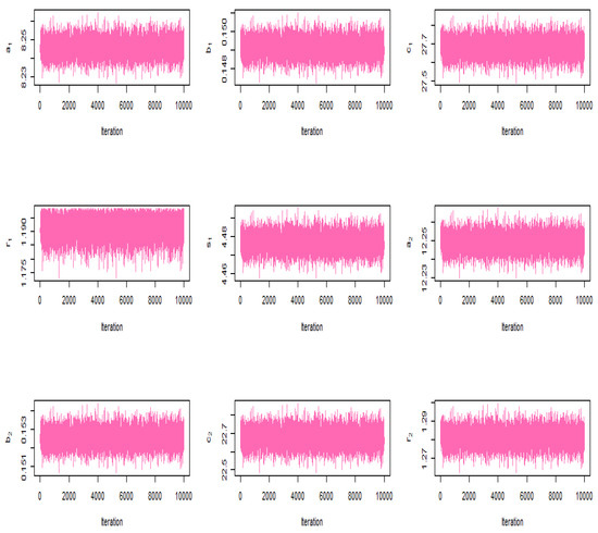
Figure 4. MCMC trace for results of Bayesian estimation of model for complete Bladder data for first 9 parameters.

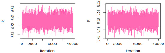
Figure 5. MCMC trace for results of Bayesian estimation of model for complete Bladder data for the last two parameters.

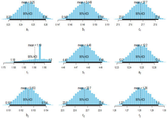
Figure 6. MCMC density and HDI intervals for results of Bayesian estimation of model for complete Bladder data for 9 parameters.

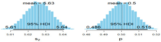
Figure 7. MCMC density and HDI intervals for the Bayesian estimation of model for complete Bladder data for the last two parameters.

Two different sampling schemes are used to generate the progressively censored samples from the bladder cancer data with m = 100, which are as follows:

Strategy 1: (99*0,28); $R_{kı}=\{\begin{array}{c}{n}_k-m_k, ı=1\\ 0, ı=2,\dots ,m_k \end{array}$ (type II censoring scheme).

Strategy 2: (28,99*0); $R_{kı}=\{\begin{array}{c}{n}_k-m_k, ı=m_k\\ 0, ı=1,\dots ,m_{k-1} \end{array}$.

In both cases, we have considered the optimization algorithm to compute the ML estimates. Table 10 shows the ML estimates for these two schemes.

Table 10. ML estimates of the MEKW parameters for different censoring schemes of the bladder data.

			MLE		Bayesian
m			Estimates	SE	Estimates	SE	Lower	Upper
100	I	1	0.7798	0.6666	2.3379	0.1443	2.0831	2.5781
		2	0.3701	0.2945	1.4005	0.1141	1.1089	1.5987
		3	1.5890	1.5642	1.0217	0.0929	0.8747	1.2007
		4	1.0476	0.3145	0.6716	0.0607	0.5607	0.8075
		5	2.5998	1.4655	6.1628	0.1388	5.9327	6.4243
		6	0.3585	0.4015	0.4015	0.0689	0.2564	0.5199
		7	0.0910	0.1559	0.3354	0.0565	0.2526	0.4543
		8	2.2788	1.9297	4.1502	0.1257	3.9216	4.3922
		9	0.8801	0.2630	0.6598	0.0461	0.5720	0.7408
		10	0.3263	0.4107	0.7023	0.1030	0.4812	0.8705
		11	0.4996	0.0312	0.4978	0.0307	0.4320	0.5622
	II	1	3.1095	1.2115	2.9865	0.8578	1.3865	4.5300
		2	5.4366	1.2115	5.5720	0.5985	4.7450	7.8209
		3	1.6154	1.5705	2.0721	0.9825	0.4263	3.9153
		4	0.3895	0.5488	0.3989	0.0817	0.2433	0.5639
		5	9.4701	3.0546	10.1271	2.1945	5.8077	14.0496
		6	3.1391	0.2030	3.2203	0.1536	2.1766	3.9201
		7	5.3816	4.7374	6.0417	2.5953	1.8477	11.4996
		8	1.6035	1.5762	1.8511	1.1209	0.4448	4.2545
		9	0.3891	0.3544	0.4127	0.1405	0.1992	0.7092
		10	9.2241	5.6376	11.1351	4.8638	3.1418	19.6341
		11	0.5000	0.0312	0.5031	0.0245	0.4146	0.5892

For Case 1, where m = 100 and under the Scheme 1, the following can be noted: 0.08 0.20 0.40 0.50 0.51 0.81 0.90 1.05 1.19 1.26 1.35 1.40 1.46 1.76 2.02 2.02 2.07 2.09 2.23 2.26 2.46 2.54 2.62 2.64 2.69 2.69 2.75 2.83 2.87 3.02 3.25 3.31 3.36 3.36 3.48 3.52 3.57 3.64 3.70 3.82 3.88 4.18 4.23 4.26 4.33 4.34 4.40 4.50 4.51 4.87 4.98 5.06 5.09 5.17 5.32 5.32 5.34 5.41 5.41 5.49 5.62 5.71 5.85 6.25 6.54 6.76 6.93 6.94 6.97 7.09 7.26 7.28 7.32 7.39 7.59 7.62 7.63 7.66 7.87 7.93 8.26 8.37 8.53 8.65 8.66 9.02 9.22 9.47 9.74 10.06 10.34 10.66 10.75 11.25 11.64 11.79 11.98 12.02 12.03 12.07.

For Case 2, where m = 100 and under the Scheme 2, the following can be noted: 0.08 0.20 0.40 0.50 0.90 1.05 1.19 1.35 1.40 1.46 1.76 2.02 2.09 2.23 2.26 2.46 2.64 2.69 2.69 2.75 2.83 3.02 3.25 3.31 3.36 3.36 3.48 3.52 3.57 3.64 3.82 4.18 4.23 4.26 4.33 4.34 4.40 4.50 4.51 4.87 4.98 5.06 5.09 5.17 5.32 5.32 5.41 5.41 5.49 5.62 5.71 6.25 6.54 6.76 6.93 6.94 6.97 7.09 7.28 7.32 7.39 7.59 7.62 7.63 7.66 8.37 8.53 8.65 9.02 9.47 9.74 10.06 10.66 10.75 11.25 11.64 11.79 11.98 12.02 12.07 12.63 13.29 14.24 14.77 16.62 17.12 17.36 18.10 19.13 20.28 22.69 23.63 25.74 25.82 26.31 34.26 36.66 43.01 46.12 79.05.

In addition, Bayesian credible interval estimates of the parameters are obtained numerically using Markov chain Monte Carlo (MCMC) techniques. That is, samples are simulated from the joint posterior distribution in Equation (12) using the Metropolis–Hasting algorithm to obtain the posterior mean values of the estimates of the parameters by MCMC. Table 10 reports the estimates of the MEKW parameters with the corresponding SE and credible confidence intervals using the HDI algorithm of the Bayesian estimators.

9. Concluding Remarks

Finite mixture models under both the continuous and the discrete domain have received considerable attention over the last decade or so due to its flexibility of modeling an observed phenomenon when each component cannot adequately explain the entire nature of the data. In this paper, we have developed and studied a finite mixture of exponentiated Kumaraswamy-G distribution under a progressively type II censored sampling scheme, when the baseline distribution (G) is a two parameter Weibull. The efficacy of the proposed model has been established through applying it to model data from the healthcare domain. From the simulation study as well as from the application, it has been observed that, depending on the censoring scheme, either of the two estimation methods (i.e., maximum likelihood and the Bayesian estimation under independent gamma priors) could be useful. Among the various loss functions assumed for the Bayesian estimation, the results based on the small simulation study are inconclusive as to which loss function will be the most suitable for this type of finite mixture models. Most likely, a full-scale simulation study with varying parameter choices and a wide range of censoring schemes would give us an idea. Currently, we are working on this and it will be published when it is ready for submission.

References

- Al Alotaibi, R.; Almetwally, E.M.; Ghosh, I.; Rezk, H. Classical and Bayesian inference on finite mixture of exponentiated Kumaraswamy Gompertz and exponentiated Kumaraswamy Frechet distributions under progressive Type II censoring with applications. Mathematics 2022, 10, 1496. [Google Scholar] [CrossRef]
- Tahir, M.H.; Nadarajah, S. Parameter induction in continuous univariate distributions: Well-established G families. Ann. Braz. Acad. Sci. 2015, 87, 539–568. [Google Scholar] [CrossRef] [PubMed]
- Lemonte, J.A.; Barreto-Souza, W.; Cordeiro, M.G. The exponentiated Kumaraswamy distribution and its log-transform. Braz. J. Probab. Stat. 2003, 27, 31–53. [Google Scholar] [CrossRef]
- Alzaghal, A.; Felix, F.; Carl, L. Exponentiated T-X family of distributions with some applications. Int. J. Stat. Probab. 2013, 2, 31–49. [Google Scholar] [CrossRef]
- Nadarajah, S.; Rocha, R. Newdistns: An R Package for new families of distributions. J. Stat. Softw. 2016, 69, 1–32. [Google Scholar] [CrossRef]
- Mudholkar, G.S.; Srivastava, D.K.; Kollia, G.D. A generalization of the Weibull distribution with application to the analysis of survival data. J. Am. Stat. Assoc. 1996, 91, 1575–1583. [Google Scholar] [CrossRef]
- Gupta, R.C.; Gupta, P.L.; Gupta, R.D. Modeling failure time data by Lehman alternatives. Comm. Statist. Theory Methods 1998, 27, 887–904. [Google Scholar] [CrossRef]
- Nadarajah, S.; Bakouch, H.S.; Tahmabi, R. Ageneralized Lindley distribution. Sankhya B 2011, 73, 331–359. [Google Scholar] [CrossRef]
- Blanchet, J.H.; Sigman, K. On exact sampling of stochastic perpetuilies. J. Appl. Probab. 2011, 48A, 165–182. [Google Scholar] [CrossRef][Green Version]
- Ali, S.; Aslam, M.; Mohsin, S.; Kazmi, A. A study of the effect of the loss function on Bayes estimate, posterior risk and hazard function for Lindley distribution. Appl. Math. Model. 2013, 23, 6068–6078. [Google Scholar] [CrossRef]
- Wasan, M.T. Parametric Estimation; Mcgraw-Hill: New York, NY, USA, 1970. [Google Scholar]
- R Core Team. R: A Language and Environment for Statistical Computing; R Foundation for Statistical Computing: Vienna, Austria, 2019; Available online: https://www.R-project.org/ (accessed on 12 July 2022).
- Lee, E.T.; Wang, J. Statistical Methods for Survival Data Analysis; John Wiley & Sons: New York, NY, USA, 2003; 476p. [Google Scholar]
- Rothenberg, T.J. Identification in Parametric Models. Econometrica 1971, 39, 577–591. [Google Scholar] [CrossRef]
Publisher’s Note: MDPI stays neutral with regard to jurisdictional claims in published maps and institutional affiliations. |
© 2022 by the authors. Licensee MDPI, Basel, Switzerland. This article is an open access article distributed under the terms and conditions of the Creative Commons Attribution (CC BY) license (https://creativecommons.org/licenses/by/4.0/).