Diverse Properties and Approximate Roots for a Novel Kinds of the (p,q)-Cosine and (p,q)-Sine Geometric Polynomials

Abstract

Utilizing $\left(p,q\right)$-numbers and $\left(p,q\right)$-concepts, in 2016, Duran et al. considered $\left(p,q\right)$-Genocchi numbers and polynomials, $\left(p,q\right)$-Bernoulli numbers and polynomials and $\left(p,q\right)$-Euler polynomials and numbers and provided multifarious formulas and properties for these polynomials. Inspired and motivated by this consideration, many authors have introduced $(p,q)$-special polynomials and numbers and have described some of their properties and applications. In this paper, using the $(p,q)$-cosine polynomials and $(p,q)$-sine polynomials, we consider a novel kinds of $(p,q)$-extensions of geometric polynomials and acquire several properties and identities by making use of some series manipulation methods. Furthermore, we compute the $\left(p,q\right)$-integral representations and $\left(p,q\right)$-derivative operator rules for the new polynomials. Additionally, we determine the movements of the approximate zerosof the two mentioned polynomials in a complex plane, utilizing the Newton method, and we illustrate them using figures.

1. Introduction

In 2016, Duran et al. [1] considered and defined $\left(p,q\right)$-Genocchi numbers and polynomials, $\left(p,q\right)$-Bernoulli polynomials and numbers and $\left(p,q\right)$-Euler numbers and polynomials. In addition, they provided many properties and formulas for these polynomials. After this study presented new extensions of some special polynomials and numbers by the $\left(p,q\right)$-numbers and $\left(p,q\right)$-concepts, many authors introduced and investigated many other $\left(p,q\right)$ generalizations of the special polynomials and numbers, such as $\left(p,q\right)$-geometric-type polynomials by Khan et al. [2], $(p,q)$-Appell type polynomials by Sadjang [3], two bivariate kinds of $\left(p,q\right)$-Bernoulli numbers and polynomials by Sadjang et al. [4], Apostol type $\left(p,q\right)$-Frobenius Eulerian polynomials by Khan et al. [5], $\left(p,q\right)$-Frobenius–Euler numbers and polynomials by Duran et al. [6] and $\left(p,q\right)$-cosine and $\left(p,q\right)$-sine geometric polynomials by Khan et al. [7]. Recently, Ryoo et al. [8] defined and introduced q-cosine and q-sine Euler polynomials and also provided some figures including the approximate roots’ movements of these polynomials. Inspired and motivated by the above studies, in this paper, utilizing the $(p,q)$-sine polynomials and $(p,q)$-cosine polynomials, we introduce new kinds of $(p,q)$-generalizations of geometric polynomials and attain diverse properties and formulas by making use of some series manipulation methods. Moreover, we develop the $\left(p,q\right)$-integral representations and $\left(p,q\right)$-derivative operator rules for these polynomials. Furthermore, we determine the movements of the approximate zerosof the mentioned novel polynomials in a complex plane using the Newton method and we indicate them in figures.

The twin-basic numbers, also termed $(p,q)$-numbers, are provided by

$${\left[m\right]}_{p,q}=\frac{p^m-q^m}{p-q},$$

for $1\ge \left|p\right|>\left|q\right|>0$ (cf. [9,10,11]).

The $(p,q)$-derivative operator of a function g with respect to $\varpi$ is given as follows

$$D_{p,q;\varpi }g\left(\varpi \right)=\frac{g\left(p\varpi \right)-g\left(q\varpi \right)}{(p-q)\varpi }(\varpi \ne 0),$$

(1)

with $\left(D_{p,q}g\left(0\right)\right)=g^{\prime }\left(0\right)$, providing that g is differentiable at 0.

The $(p,q)$-extension of the binomial coefficients is introduced as follows

$${\left(\genfrac{}{}{0pt}{}{m}{\nu }\right)}_{p,q}={\displaystyle \frac{{\left[m\right]}_{p,q}!}{{\left[\nu \right]}_{p,q}!{[m-\nu ]}_{p,q}!}}(m\ge \nu ),$$

where the $(p,q)$-analogs of the factorial numbers ${\left[m\right]}_{p,q}!$ are given by

$${\left[m\right]}_{p,q}!={\left[m\right]}_{p,q}\cdots {\left[2\right]}_{p,q}{\left[1\right]}_{p,q}\mathrm{for}m\in \mathbb{N}\mathrm{with}{\left[0\right]}_{p,q}:=1.$$

The $(p,q)$-extension of addition ${\left(\varpi +a\right)}^m$ is given as follows

$${\left(\varpi {\oplus }_{p,q}a\right)}^m:=(\varpi +a)(p\varpi +aq)\cdots (p^{m-1}\varpi +a{q}^{m-1})\mathrm{for}m\ge 1$$

with ${\left(\varpi {\oplus }_{p,q}a\right)}^0:=1$ and this also has the following expansion

$${\left(\varpi {\oplus }_{p,q}a\right)}^m=\sum _{\nu =0}^m{p}^{\left(\genfrac{}{}{0pt}{}{m}{2}\right)}{q}^{\left(\genfrac{}{}{0pt}{}{m-\nu }{2}\right)}{a}^{m-\nu }{\varpi }^{\nu }{\left(\genfrac{}{}{0pt}{}{m}{\nu }\right)}_{p,q}.$$

(2)

The $(p,q)$-extension of subtraction ${\left(\varpi -a\right)}^m$ is provided as follows

$${\left(\varpi {\ominus }_{p,q}a\right)}^m:=(\varpi -a)(p\varpi -aq)\cdots (p^{m-1}\varpi -a{q}^{m-1})\mathrm{for}m\ge 1$$

with ${\left(\varpi {\ominus }_{p,q}a\right)}^0:=1$ and this also has the following expansion

$${\left(\varpi {\ominus }_{p,q}a\right)}^m=\sum _{\nu =0}^m{p}^{\left(\genfrac{}{}{0pt}{}{m}{2}\right)}{q}^{\left(\genfrac{}{}{0pt}{}{m-\nu }{2}\right)}{\left(-a\right)}^{m-\nu }{\varpi }^{\nu }{\left(\genfrac{}{}{0pt}{}{m}{\nu }\right)}_{p,q}.$$

(3)

The $(p,q)$-analogs of the exponential functions, $e_{p,q}\left(\varpi \right)$ and $E_{p,q}\left(\varpi \right)$, are provided as follows:

$$e_{p,q}\left(\varpi \right)=\sum _{m=0}^{\infty }\frac{p^{\left(\genfrac{}{}{0pt}{}{m}{2}\right)}{\varpi }^m}{{\left[m\right]}_{p,q}!}\mathrm{and}{E}_{p,q}\left(\varpi \right)=\sum _{m=0}^{\infty }\frac{q^{\left(\genfrac{}{}{0pt}{}{m}{2}\right)}{\varpi }^m}{{\left[m\right]}_{p,q}!},$$

(4)

which have the following relationships

$$e_{p,q}\left(\varpi \right)E_{p,q}(-\varpi )=1\mathrm{and}{e}_{p^{-1}{q}^{-1}}\left(\varpi \right)=E_{p,q}\left(\varpi \right),$$

(5)

and the following rules

$$D_{p,q}{e}_{p,q}\left(\varpi \right)=e_{p,q}\left(p\varpi \right)\mathrm{and}{D}_{p,q}{E}_{p,q}\left(\varpi \right)=E_{p,q}\left(q\varpi \right).$$

(6)

We observe that

$$e_{p,q}\left(\varpi {\oplus }_{p,q}\vartheta \right)=E_{p,q}\left(\vartheta \right)e_{p,q}\left(\varpi \right).$$

(7)

The $(p,q)$-definite integral is provided (cf. [11]) as follows:

$${\int }_0^{j}g\left(\varpi \right)d_{p,q}\varpi =j(p-q)\sum _{\nu =0}^{\infty }\frac{p^{\nu }}{q^{\nu +1}}g\left(j\frac{p^{\nu }}{q^{\nu +1}}\right)$$

in conjunction with

$${\int }_h^{j}g\left(\varpi \right)d_{p,q}\varpi ={\int }_0^{j}g\left(\varpi \right)d_{p,q}\varpi -{\int }_0^{h}g\left(\varpi \right)d_{p,q}\varpi .$$

(8)

The $(p,q)$-generalizations of the sine functions and the cosine functions are provided (cf. [4]) as follows:

$$\begin{array}{cc}{\displaystyle \sum _{m=0}^{\infty }}\frac{{(-1)}^m{p}^{\left(\genfrac{}{}{0pt}{}{2m+1}{2}\right)}{\varpi }^{2m+1}}{{[2m+1]}_{p,q}!}={sin}_{p,q}\left(\varpi \right),& {\displaystyle \sum _{m=0}^{\infty }}\frac{{(-1)}^m{p}^{\left(\genfrac{}{}{0pt}{}{m}{2}\right)}{\varpi }^{2m}}{{\left[2m\right]}_{p,q}!}={cos}_{p,q}\left(\varpi \right),\\ {\displaystyle \sum _{m=0}^{\infty }}\frac{{(-1)}^m{q}^{\left(\genfrac{}{}{0pt}{}{2m+1}{2}\right)}{\varpi }^{2m+1}}{{[2m+1]}_{p,q}!}={SIN}_{p,q}\left(\varpi \right),& {\displaystyle \sum _{m=0}^{\infty }}\frac{{(-1)}^m{q}^{\left(\genfrac{}{}{0pt}{}{m}{2}\right)}{\varpi }^{2m}}{{\left[2m\right]}_{p,q}!}=COS{}_{p,q}\left(\varpi \right).\end{array}$$

(9)

From (4) and (9), we can easily observe that

$$e_{p,q}\left(i\varpi \right)={cos}_{p,q}\left(\varpi \right)+i{sin}_{p,q}\left(\varpi \right)\mathrm{and}{E}_{p,q}\left(i\varpi \right)=COS{}_{p,q}\left(\varpi \right)+i{SIN}_{p,q}\left(\varpi \right),$$

(10)

which are the $\left(p,q\right)$-extensions of the classical Euler formula $e^{i\varpi }=cos\varpi +isin\varpi$, where $i^2=-1$ and $\varpi \in \mathbb{R}$.

2. On $(\mathit{p},\mathit{q})$-Extensions of Geometric Polynomials

The geometric polynomials, also termed Fubini polynomials, are provided by (cf. [12,13]):

$$\frac{1}{1-\varpi (e^t-1)}=\sum _{m=0}^{\infty }{F}_m\left(\varpi \right)\frac{t^m}{m!},$$

(11)

which gives

$$F_m\left(\varpi \right)=\sum _{\nu =0}^m{S}_2\left(m,\nu \right)\nu !{\varpi }^{\nu },$$

(12)

where the notation $S_2\left(m,\nu \right)$, known as the Stirling numbers of the second kind, are defined as follows (cf. [14,15]):

$$\frac{{(e^t-1)}^{\nu }}{\nu !}=\sum _{m=0}^{\infty }{S}_2\left(m,\nu \right)\frac{t^m}{m!}.$$

Letting $\varpi =1$, we acquire $F_m\left(1\right):=F_m$, which shows the corresponding geometric numbers.

Khan et al. [2] considered the three variable $\left(p,q\right)$-geometric polynomials as follows:

$$\frac{e_{p,q}\left(\varpi t\right)E_{p,q}\left(\vartheta t\right)}{1-\kappa (e_{p,q}\left(t\right)-1)}=\sum _{m=0}^{\infty }{F}_m(\varpi ,\vartheta ;\kappa :p,q)\frac{t^m}{{\left[m\right]}_{p,q}!}.$$

(13)

Taking $\vartheta =0$ in (13), we attain the two variable $\left(p,q\right)$-geometric polynomials provided by

$$\frac{e_{p,q}\left(\varpi t\right)}{1-\kappa (e_{p,q}\left(t\right)-1)}=\sum _{m=0}^{\infty }{F}_m(\varpi ;\kappa :p,q)\frac{t^m}{{\left[m\right]}_{p,q}!}.$$

(14)

The Maclaurin series expansions of $e^{\varpi t}sin\left(\vartheta t\right)$ and $e^{\varpi t}cos\left(\vartheta t\right)$, are developed as follows (cf. [16]):

$$e^{\varpi t}sin\vartheta t=\sum _{m=0}^{\infty }{S}_m(\varpi ,\vartheta )\frac{t^m}{m!}\mathrm{and}{e}^{\varpi t}cos\vartheta t=\sum _{m=0}^{\infty }{C}_m(\varpi ,\vartheta )\frac{t^m}{m!},$$

(15)

where

$$S_m(\varpi ,\vartheta )=\sum _{\nu =0}^{⌊\frac{m-1}{2}⌋}\left(\genfrac{}{}{0pt}{}{m}{2\nu +1}\right){\varpi }^{m-2\nu -1}{(-1)}^{\nu }{\vartheta }^{2\nu +1}\mathrm{and}{C}_m(\varpi ,\vartheta )=\sum _{\nu =0}^{⌊\frac{m}{2}⌋}{(-1)}^{\nu }\left(\genfrac{}{}{0pt}{}{m}{2\nu }\right){\varpi }^{m-2\nu }{\vartheta }^{2\nu }.$$

(16)

Recently, Sadjang et al. [4] introduced and investigated $(p,q)$-extensions of $S_m(\varpi ,\vartheta )$ and $C_m(\varpi ,\vartheta )$:

$${sin}_{p,q}\left(\vartheta t\right)e_{p,q}\left(\varpi t\right)=\sum _{m=0}^{\infty }{S}_{m,p,q}(\varpi ,\vartheta )\frac{t^m}{{\left[m\right]}_{p,q}!}$$

(17)

and

$${cos}_{p,q}\left(\vartheta t\right)e_{p,q}\left(\varpi t\right)=\sum _{m=0}^{\infty }{C}_{m,p,q}(\varpi ,\vartheta )\frac{t^m}{{\left[m\right]}_{p,q}!},$$

(18)

where

$$S_{m,p,q}(\varpi ,\vartheta )=\sum _{\nu =0}^{⌊\frac{m-1}{2}⌋}{(-1)}^{\nu }{\left(\genfrac{}{}{0pt}{}{m}{2\nu +1}\right)}_{p,q}{p}^{\left(4{\nu }^2-2\right)+\left(\genfrac{}{}{0pt}{}{m-1}{2}\right)}{\varpi }^{m-2\nu -1}{\vartheta }^{2\nu +1}$$

(19)

and

$$C_{m,p,q}(\varpi ,\vartheta )=\sum _{\nu =0}^{⌊\frac{m}{2}⌋}{(-1)}^{\nu }{\left(\genfrac{}{}{0pt}{}{m}{2\nu }\right)}_{p,q}{p}^{\left(\genfrac{}{}{0pt}{}{m}{2}\right)+2\nu (\nu -m)}{\varpi }^{m-2\nu }{\vartheta }^{2\nu }.$$

(20)

Motivated by the above, we now define new kinds of the $(p,q)$-extensions of $S_m(\varpi ,\vartheta )$ and $C_m(\varpi ,\vartheta )$ as follows

$$\sum _{m=0}^{\infty }{\mathcal{S}}_{m,p,q}(\varpi ,\vartheta )\frac{t^m}{{\left[m\right]}_{p,q}!}={SIN}_{p,q}\left(\vartheta t\right)e_{p,q}\left(\varpi t\right)$$

(21)

and

$$\sum _{m=0}^{\infty }{\mathcal{C}}_{m,p,q}(\varpi ,\vartheta )\frac{t^m}{{\left[m\right]}_{p,q}!}={COS}_{p,q}\left(\vartheta t\right)e_{p,q}\left(\varpi t\right),$$

(22)

which readily yields the following explicit formulas:

$${\mathcal{S}}_{m,p,q}(\varpi ,\vartheta )=\sum _{\nu =0}^{⌊\frac{m-1}{2}⌋}{(-1)}^{\nu }{p}^{\left(\genfrac{}{}{0pt}{}{m-2\nu -1}{2}\right)}{\left(\genfrac{}{}{0pt}{}{m}{2\nu +1}\right)}_{p,q}{q}^{\left(\genfrac{}{}{0pt}{}{2\nu +1}{2}\right)}{\varpi }^{m-2\nu -1}{\vartheta }^{2\nu +1}$$

and

$${\mathcal{C}}_{m,p,q}(\varpi ,\vartheta )=\sum _{\nu =0}^{⌊\frac{m}{2}⌋}{(-1)}^{\nu }{\left(\genfrac{}{}{0pt}{}{m}{2\nu }\right)}_{p,q}{p}^{\left(\genfrac{}{}{0pt}{}{m-2\nu }{2}\right)}{q}^{\left(\genfrac{}{}{0pt}{}{2\nu }{2}\right)}{\varpi }^{m-2\nu }{\vartheta }^{2\nu }.$$

Recently, the $(p,q)$-extensions of the sine-geometric polynomials and cosine-geometric polynomials $F_m^{\left(s\right)}(\varpi ,\vartheta ;\kappa :p,q)$ and $F_m^{\left(c\right)}(\varpi ,\vartheta ;\kappa :p,q)$ are considered (cf. [7]) as follows:

$$\frac{{sin}_{p,q}\left(\vartheta t\right)e_{p,q}\left(\varpi t\right)}{1-\kappa (e_{p,q}\left(t\right)-1)}=\sum _{m=0}^{\infty }{\mathcal{F}}_m^{\left(s\right)}(\varpi ,\vartheta ;\kappa :p,q)\frac{t^m}{{\left[m\right]}_{p,q}!}$$

(23)

and

$$\frac{{cos}_{p,q}\left(\vartheta t\right)e_{p,q}\left(\varpi t\right)}{1-\kappa (e_{p,q}\left(t\right)-1)}=\sum _{m=0}^{\infty }{\mathcal{F}}_m^{\left(c\right)}(\varpi ,\vartheta ;\kappa :p,q)\frac{t^m}{{\left[m\right]}_{p,q}!}$$

(24)

for $q,p\in \mathbb{C}$, providing that $1\ge \left|p\right|>\left|q\right|>0$. Then, several properties were derived in [7].

3. New Kinds of $(\mathit{p},\mathit{q})$-Cosine and $(\mathit{p},\mathit{q})$-Sine Geometric Polynomials

Motivated and inspired by definitions (23) and (24), we consider the following definition.

Definition 1.

We introduce novel kinds of $(p,q)$-sine and $(p,q)$-cosine geometric polynomials, for $q,p\in \mathbb{C}$, providing that $1\ge \left|p\right|>\left|q\right|>0$, as follows:

$$\sum _{m=0}^{\infty }{\mathfrak{F}}_m^{\left(S\right)}\left(\varpi ,\vartheta ;\kappa :p,q\right)\frac{t^m}{{\left[m\right]}_{p,q}!}=\frac{e_{p,q}\left(\varpi t\right){SIN}_{p,q}\left(\vartheta t\right)}{1-\kappa (e_{p,q}\left(t\right)-1)}$$

(25)

and

$$\sum _{m=0}^{\infty }{\mathfrak{F}}_m^{\left(C\right)}\left(\varpi ,\vartheta ;\kappa :p,q\right)\frac{t^m}{{\left[m\right]}_{p,q}!}=\frac{e_{p,q}\left(\varpi t\right){COS}_{p,q}\left(\vartheta t\right)}{1-\kappa (e_{p,q}\left(t\right)-1)}.$$

(26)

Letting $\vartheta =0$ in (23) and (24), we attain two variables, the $(p,q)$-geometric polynomials $F_m(\varpi ;\kappa :p,q)$ provided as follows (cf. [2]) that

$$\frac{e_{p,q}\left(\varpi t\right)}{1-\kappa (e_{p,q}\left(t\right)-1)}=\sum _{m=0}^{\infty }{F}_m(\varpi ;\kappa :p,q)\frac{t^m}{{\left[m\right]}_{p,q}!}.$$

(27)

When $\varpi =\vartheta =0$ in (23) and (24), we acquire the familiar $(p,q)$-geometric polynomials $F_m(\kappa :p,q)$ provided as follows that

$$\frac{1}{1-\kappa (e_{p,q}\left(t\right)-1)}=\sum _{m=0}^{\infty }{F}_m(\kappa :p,q)\frac{t^m}{{\left[m\right]}_{p,q}!}$$

and setting $\varpi =\vartheta =0$ and $\kappa =1$ in (23) and (24), we acquire the usual $(p,q)$-geometric numbers $F_m(p,q)$ provided as follows (cf. [2]) that

$$\frac{1}{2-e_{p,q}\left(t\right)}=\sum _{m=0}^{\infty }{F}_m(p,q)\frac{t^m}{{\left[m\right]}_{p,q}!}.$$

Here we can provide the consideration of Definition 1 arising from the two variables, the $(p,q)$-geometric polynomials $F_m(\varpi ;\kappa :p,q)$, as follows.

Theorem 1.

The following identities hold:

$$\frac{e_{p,q}\left(\varpi t\right){SIN}_{p,q}\left(\vartheta t\right)}{1-\kappa (e_{p,q}\left(t\right)-1)}=\sum _{m=0}^{\infty }\left(\frac{F_m(\left(\varpi {\oplus }_{p,q}i\vartheta \right);\kappa :p,q)-F_m(\left(\varpi {\ominus }_{p,q}i\vartheta \right);\kappa :p,q)}{2i}\right)\frac{t^m}{{\left[m\right]}_{p,q}!}$$

(28)

and

$$\frac{e_{p,q}\left(\varpi t\right){COS}_{p,q}\left(\vartheta t\right)}{1-\kappa (e_{p,q}\left(t\right)-1)}=\sum _{m=0}^{\infty }\left(\frac{F_m(\left(\varpi {\oplus }_{p,q}i\vartheta \right);\kappa :p,q)+F_m(\left(\varpi {\ominus }_{p,q}i\vartheta \right);\kappa :p,q)}{2}\right)\frac{t^m}{{\left[m\right]}_{p,q}!},$$

(29)

for $i^2=-1$ and $\varpi \in \mathbb{R}$.

Proof. 

From (14), (7) and Definition 1, we can observe that

$$\begin{array}{c}\sum _{m=0}^{\infty }{F}_m(\left(\varpi {\oplus }_{p,q}i\vartheta \right);\kappa :p,q)\frac{t^m}{{\left[m\right]}_{p,q}!}=\frac{e_{p,q}\left(\left(\varpi {\oplus }_{p,q}i\vartheta \right)t\right)}{1-\kappa (e_{p,q}\left(t\right)-1)}\\ =\frac{e_{p,q}\left(\varpi t\right)E_{p,q}\left(i\vartheta t\right)}{1-\kappa (e_{p,q}\left(t\right)-1)}\\ =\frac{\left({COS}_{p,q}\left(\vartheta t\right)+iSIN{}_{p,q}\left(\vartheta t\right)\right)e_{p,q}\left(\varpi t\right)}{1-\kappa (e_{p,q}\left(t\right)-1)}\end{array}$$

and similarly

$$\begin{array}{c}\sum _{m=0}^{\infty }{F}_m(\left(\varpi {\ominus }_{p,q}i\vartheta \right);\kappa :p,q)\frac{t^m}{{\left[m\right]}_{p,q}!}=\frac{e_{p,q}\left(\left(\varpi {\ominus }_{p,q}i\vartheta \right)t\right)}{1-\kappa (e_{p,q}\left(t\right)-1)}\\ =\frac{E_{p,q}(-i\vartheta t)e_{p,q}\left(\varpi t\right)}{1-\kappa (e_{p,q}\left(t\right)-1)}\\ =\frac{\left({COS}_{p,q}\left(\vartheta t\right)-iSIN{}_{p,q}\left(\vartheta t\right)\right)e_{p,q}\left(\varpi t\right)}{1-\kappa (e_{p,q}\left(t\right)-1)},\end{array}$$

which complete the proofs of (28) and (29). □

Remark 1.

According to Theorem 1 and Definition 1, we can observe that

$$\frac{F_m(\left(\varpi {\oplus }_{p,q}i\vartheta \right);\kappa :p,q)-F_m(\left(\varpi {\ominus }_{p,q}i\vartheta \right);\kappa :p,q)}{2i}={\mathfrak{F}}_m^{\left(S\right)}\left(\varpi ,\vartheta ;\kappa :p,q\right)$$

and

$$\frac{F_m(\left(\varpi {\oplus }_{p,q}i\vartheta \right);\kappa :p,q)+F_m(\left(\varpi {\ominus }_{p,q}i\vartheta \right);\kappa :p,q)}{2}={\mathfrak{F}}_m^{\left(C\right)}\left(\varpi ,\vartheta ;\kappa :p,q\right).$$

Theorem 2.

We have

$$\sum _{\nu =0}^m{\left(\genfrac{}{}{0pt}{}{m}{\nu }\right)}_{p,q}{\mathcal{S}}_{m-\nu ,p,q}(\varpi ,\vartheta )F_{\nu ,p,q}\left(\kappa \right)={\mathfrak{F}}_m^{\left(S\right)}\left(\varpi ,\vartheta ;\kappa :p,q\right)$$

(30)

and

$$\sum _{\nu =0}^m{\left(\genfrac{}{}{0pt}{}{m}{\nu }\right)}_{p,q}{\mathcal{C}}_{m-\nu ,p,q}(\varpi ,\vartheta )F_{\nu ,p,q}\left(\kappa \right)={\mathfrak{F}}_m^{\left(C\right)}\left(\varpi ,\vartheta ;\kappa :p,q\right)$$

(31)

which hold for $\varpi ,\vartheta \in \mathbb{R}$ and $q,p\in \mathbb{C}$ provided that $1\ge \left|p\right|>\left|q\right|>0$.

Proof. 

In view of (25) and (26), making use of (21) and (22), we can obviously observe that

$$\begin{array}{c}\sum _{m=0}^{\infty }{\mathfrak{F}}_m^{\left(S\right)}(\varpi ,\vartheta ;\kappa :p,q)\frac{t^m}{{\left[m\right]}_{p,q}!}=\frac{e_{p,q}\left(\varpi t\right)SIN{}_{p,q}\left(\vartheta t\right)}{1-\kappa (e_{p,q}\left(t\right)-1)}\\ =\left(\sum _{m=0}^{\infty }{\mathcal{S}}_{m,p,q}(\varpi ,\vartheta )\frac{t^m}{{\left[m\right]}_{p,q}!}\right)\left(\sum _{m=0}^{\infty }{F}_m(p,q)\frac{t^m}{{\left[m\right]}_{p,q}!}\right)\\ =\sum _{m=0}^{\infty }\left(\sum _{\nu =0}^m{\left(\genfrac{}{}{0pt}{}{m}{\nu }\right)}_{p,q}{F}_{\nu ,p,q}\left(\kappa \right){\mathcal{S}}_{m-\nu ,p,q}(\varpi ,\vartheta )\right)\frac{t^m}{{\left[m\right]}_{p,q}!}\end{array}$$

and

$$\begin{array}{c}\sum _{m=0}^{\infty }{\mathfrak{F}}_m^{\left(C\right)}(\varpi ,\vartheta ;\kappa :p,q)\frac{t^m}{{\left[m\right]}_{p,q}!}=\frac{e_{p,q}\left(\varpi t\right)COS{}_{p,q}\left(\vartheta t\right)}{1-\kappa (e_{p,q}\left(t\right)-1)}\\ =\left(\sum _{m=0}^{\infty }{\mathcal{C}}_{m,p,q}(\varpi ,\vartheta )\frac{t^m}{{\left[m\right]}_{p,q}!}\right)\left(\sum _{m=0}^{\infty }{F}_m(p,q)\frac{t^m}{{\left[m\right]}_{p,q}!}\right)\\ =\sum _{m=0}^{\infty }\left(\sum _{\nu =0}^m{\left(\genfrac{}{}{0pt}{}{m}{\nu }\right)}_{p,q}{F}_{\nu ,p,q}\left(\kappa \right){\mathcal{C}}_{m-\nu ,p,q}(\varpi ,\vartheta )\right)\frac{t^m}{{\left[m\right]}_{p,q}!},\end{array}$$

which gives the claimed Formulas (30) and (31). □

Theorem 3.

Let $q,p\in \mathbb{C}$ provide $1\ge \left|p\right|>\left|q\right|>0$ and $0\le m$. The following relations are valid:

$${\mathfrak{F}}_m^{\left(S\right)}(\varpi ,\vartheta ;\kappa :p,q)=\sum _{k=0}^{⌊\frac{m-1}{2}⌋}{\left(\genfrac{}{}{0pt}{}{m}{2k+1}\right)}_{p,q}{F}_{m-1-2k}(\varpi ;\kappa :p,q)q^{\left(\genfrac{}{}{0pt}{}{2k+1}{2}\right)}{\vartheta }^{2k+1}{(-1)}^k$$

(32)

and

$${\mathfrak{F}}_m^{\left(C\right)}(\varpi ,\vartheta ;\kappa :p,q)=\sum _{k=0}^{⌊\frac{m}{2}⌋}{\left(\genfrac{}{}{0pt}{}{m}{2k}\right)}_{p,q}{F}_{m-2k}(\varpi ;\kappa :p,q)q^{\left(\genfrac{}{}{0pt}{}{2k}{2}\right)}{\vartheta }^{2k}{(-1)}^k.$$

(33)

Proof. 

In terms of (23) and (24), making use of (9), it can be obviously seen that

$$\begin{array}{c}\sum _{m=0}^{\infty }{\mathfrak{F}}_m^{\left(S\right)}(\varpi ,\vartheta ;\kappa :p,q)\frac{t^m}{{\left[m\right]}_{p,q}!}=\frac{SIN{}_{p,q}\left(\vartheta t\right)e_{p,q}\left(\varpi t\right)}{1-\kappa (e_{p,q}\left(t\right)-1)}\\ =\left(\sum _{m=0}^{\infty }\frac{{(-1)}^m{q}^{\left(\genfrac{}{}{0pt}{}{2m+1}{2}\right)}{\left(\vartheta t\right)}^{2m+1}}{{[2m+1]}_{p,q}!}\right)\left(\sum _{m=0}^{\infty }{F}_m^{\left(s\right)}(\varpi ;\kappa :p,q)\frac{t^m}{{\left[m\right]}_{p,q}!}\right)\\ =\sum _{m=0}^{\infty }\left(\sum _{\nu =0}^{⌊\frac{m}{2}⌋}{(-1)}^{\nu }{\left(\genfrac{}{}{0pt}{}{m}{2\nu +1}\right)}_{p,q}{q}^{\left(\genfrac{}{}{0pt}{}{2\nu +1}{2}\right)}{F}_{m-1-2\nu }(\varpi ;\kappa :p,q){\vartheta }^{2\nu +1}\right)\frac{t^m}{{\left[m\right]}_{p,q}!}\end{array}$$

and

$$\begin{array}{c}\sum _{m=0}^{\infty }{\mathfrak{F}}_m^{\left(C\right)}(\varpi ,\vartheta ;\kappa :p,q)\frac{t^m}{{\left[m\right]}_{p,q}!}=\frac{COS{}_{p,q}\left(\vartheta t\right)e_{p,q}\left(\varpi t\right)}{1-\kappa (e_{p,q}\left(t\right)-1)}\\ =\left(\sum _{m=0}^{\infty }\frac{{(-1)}^m{q}^{\left(\genfrac{}{}{0pt}{}{m}{2}\right)}{\varpi }^{2m}}{{\left[2m\right]}_{p,q}!}\right)\left(\sum _{m=0}^{\infty }{F}_m^{\left(s\right)}(\varpi ;\kappa :p,q)\frac{t^m}{{\left[m\right]}_{p,q}!}\right)\\ =\sum _{m=0}^{\infty }\left(\sum _{\nu =0}^{⌊\frac{m}{2}⌋}{F}_{m-2\nu }(\varpi ;\kappa :p,q){(-1)}^{\nu }{\left(\genfrac{}{}{0pt}{}{m}{2\nu }\right)}_{p,q}{q}^{\left(\genfrac{}{}{0pt}{}{2\nu }{2}\right)}{\vartheta }^{2\nu }\right)\frac{t^m}{{\left[m\right]}_{p,q}!},\end{array}$$

which conclude the proofs of the claimed relations (32) and (33). □

Theorem 4.

Let $q,p\in \mathbb{C}$ provided that $1\ge \left|p\right|>\left|q\right|>0$ and $0\le m$. The following correlations are valid:

$${\mathcal{S}}_{m,p,q}(\varpi ,\vartheta )=\kappa \sum _{\nu =0}^m{p}^{\left(\genfrac{}{}{0pt}{}{m-\nu }{2}\right)}{\left(\genfrac{}{}{0pt}{}{m}{\nu }\right)}_{p,q}{\mathfrak{F}}_{\nu }^{\left(S\right)}(\varpi ,\vartheta ;\kappa :p,q)-\left(\kappa +1\right){\mathfrak{F}}_m^{\left(S\right)}(\varpi ,\vartheta ;\kappa :p,q)$$

(34)

and

$${\mathcal{C}}_{m,p,q}(\varpi ,\vartheta )=\kappa \sum _{\nu =0}^m{p}^{\left(\genfrac{}{}{0pt}{}{m-\nu }{2}\right)}{\left(\genfrac{}{}{0pt}{}{m}{\nu }\right)}_{p,q}{\mathfrak{F}}_{\nu }^{\left(C\right)}(\varpi ,\vartheta ;\kappa :p,q)-\left(\kappa +1\right){\mathfrak{F}}_m^{\left(C\right)}(\varpi ,\vartheta ;\kappa :p,q).$$

(35)

Proof. 

Making use of (17), (18), (23) and (24), the proofs of (34) and (35) are based upon the equalities provided below:

$$\frac{\kappa +1{-}_{p,q}\left(t\right)}{1-\kappa (e_{p,q}\left(t\right)-1)}SIN{}_{p,q}\left(\vartheta t\right)e_{p,q}\left(\varpi t\right)=SIN{}_{p,q}\left(\vartheta t\right)e_{p,q}\left(\varpi t\right)$$

and

$$\frac{\kappa +1{-}_{p,q}\left(t\right)}{1-\kappa (e_{p,q}\left(t\right)-1)}COS{}_{p,q}\left(\vartheta t\right)e_{p,q}\left(\varpi t\right)=COS{}_{p,q}\left(\vartheta t\right)e_{p,q}\left(\varpi t\right).$$

So, we can skip the elaborations. □

Theorem 5.

Let $q,p\in \mathbb{C}$ provided that $1\ge \left|p\right|>\left|q\right|>0$ and $0\le m$. The following identities are valid:

$$\kappa {\mathfrak{F}}_m^{\left(S\right)}(\left(\varpi {\oplus }_{p,q}1\right),\vartheta ;\kappa :p,q)+{\mathcal{S}}_{m,p,q}(\varpi ,\vartheta )=\left(\kappa +1\right){\mathfrak{F}}_m^{\left(S\right)}\left(\varpi ,\vartheta ;\kappa :p,q\right)$$

(36)

and

$$\kappa {\mathfrak{F}}_m^{\left(C\right)}(\left(\varpi {\oplus }_{p,q}1\right),\vartheta ;\kappa :p,q)+{\mathcal{C}}_{m,p,q}(\varpi ,\vartheta )=\left(\kappa +1\right){\mathfrak{F}}_m^{\left(C\right)}\left(\varpi ,\vartheta ;\kappa :p,q\right).$$

(37)

Proof. 

Making use of (17), (18), (23) and (24), we can observe that

$$\begin{array}{c}\sum _{m=0}^{\infty }\left[{\mathfrak{F}}_m^{\left(S\right)}(\left(\varpi {\oplus }_{p,q}1\right),\vartheta ;\kappa :p,q)-{\mathfrak{F}}_m^{\left(S\right)}(\varpi ,\vartheta ;\kappa :p,q)\right]\frac{t^m}{{\left[m\right]}_{p,q}!}\\ =\frac{{SIN}_{p,q}\left(\vartheta t\right)e_{p,q}\left(\varpi t\right)}{1-\kappa (e_{p,q}\left(t\right)-1)}\left(e_{p,q}\left(t\right)-1\right)\\ =\frac{1}{\kappa }\left(\frac{e_{p,q}\left(\varpi t\right){SIN}_{p,q}\left(\vartheta t\right)}{1-\kappa (e_{p,q}\left(t\right)-1)}-e_{p,q}\left(\varpi t\right){SIN}_{p,q}\left(\vartheta t\right)\right)\\ =\frac{1}{\kappa }\left(\sum _{m=0}^{\infty }{\mathfrak{F}}_m^{\left(S\right)}\left(\varpi ,\vartheta ;\kappa :p,q\right)\frac{t^m}{{\left[m\right]}_{p,q}!}-\sum _{m=0}^{\infty }{\mathcal{S}}_{m,p,q}(\varpi ,\vartheta )\frac{t^m}{{\left[m\right]}_{p,q}!}\right)\end{array}$$

and

$$\begin{array}{c}\sum _{m=0}^{\infty }\left[{\mathfrak{F}}_m^{\left(C\right)}(\left(\varpi {\oplus }_{p,q}1\right),\vartheta ;\kappa :p,q)-{\mathfrak{F}}_m^{\left(C\right)}(\varpi ,\vartheta ;\kappa :p,q)\right]\frac{t^m}{{\left[m\right]}_{p,q}!}\\ =\frac{COS{}_{p,q}\left(\vartheta t\right)e_{p,q}\left(\varpi t\right)}{1-\kappa (e_{p,q}\left(t\right)-1)}\left(e_{p,q}\left(t\right)-1\right)\\ =\frac{1}{\kappa }\left(\frac{e_{p,q}\left(\varpi t\right)COS{}_{p,q}\left(\vartheta t\right)}{1-\kappa (e_{p,q}\left(t\right)-1)}-e_{p,q}\left(\varpi t\right)COS{}_{p,q}\left(\vartheta t\right)\right)\\ =\frac{1}{\kappa }\left(\sum _{m=0}^{\infty }{\mathfrak{F}}_m^{\left(C\right)}\left(\varpi ,\vartheta ;\kappa :p,q\right)\frac{t^m}{{\left[m\right]}_{p,q}!}-\sum _{m=0}^{\infty }{\mathcal{C}}_{m,p,q}(\varpi ,\vartheta )\frac{t^m}{{\left[m\right]}_{p,q}!}\right),\end{array}$$

which complete the proofs. □

Some derivative and integral properties are presented as follows.

Theorem 6.

Let $q,p\in \mathbb{C}$ provided that $1\ge \left|p\right|>\left|q\right|>0$ and $0<m$. The following rules are valid:

$$\begin{array}{c}{\mathfrak{F}}_{m-1}^{\left(S\right)}(p\varpi ,\vartheta ;\kappa :p,q){\left[m\right]}_{p,q}=\frac{\partial }{{\partial }_{p,q}\varpi }{\mathfrak{F}}_m^{\left(S\right)}(\varpi ,\vartheta ;\kappa :p,q)\\ {\mathfrak{F}}_{m-1}^{\left(S\right)}(\varpi ,q\vartheta ;\kappa :p,q){\left[m\right]}_{p,q}=\frac{\partial }{{\partial }_{p,q}\vartheta }{\mathfrak{F}}_m^{\left(S\right)}(\varpi ,\vartheta ;\kappa :p,q)\\ {\mathfrak{F}}_{m-1}^{\left(C\right)}(p\varpi ,\vartheta ;\kappa :p,q){\left[m\right]}_{p,q}=\frac{\partial }{{\partial }_{p,q}\varpi }{\mathfrak{F}}_m^{\left(C\right)}(\varpi ,\vartheta ;\kappa :p,q)\\ {\mathfrak{F}}_{m-1}^{\left(C\right)}(\varpi ,q\vartheta ;\kappa :p,q){\left[m\right]}_{p,q}=\frac{\partial }{{\partial }_{p,q}\vartheta }{\mathfrak{F}}_m^{\left(C\right)}(\varpi ,\vartheta ;\kappa :p,q).\end{array}$$

(38)

Proof. 

Applying the $\left(p,q\right)$-derivative operator to (23) with respect to $\varpi$, and also making use of (6), it can be obviously seen that

$$\begin{array}{c}\sum _{m=0}^{\infty }\frac{\partial }{{\partial }_{p,q}\varpi }{\mathfrak{F}}_m^{\left(S\right)}(\varpi ,\vartheta ;\kappa :p,q)\frac{t^m}{{\left[m\right]}_{p,q}!}=\frac{SIN{}_{p,q}\left(\vartheta t\right)\frac{\partial }{{\partial }_{p,q}\varpi }{e}_{p,q}\left(\varpi t\right)}{1-\kappa (e_{p,q}\left(t\right)-1)}\\ =t\frac{SIN{}_{p,q}\left(\vartheta t\right)e_{p,q}\left(p\varpi t\right)}{1-\kappa (e_{p,q}\left(t\right)-1)}\\ =\sum _{m=0}^{\infty }{\mathfrak{F}}_m^{\left(S\right)}(p\varpi ,\vartheta ;\kappa :p,q)\frac{t^{m+1}}{{\left[m\right]}_{p,q}!},\end{array}$$

which gives the first rule. The other rules can easily be derived in the same way. □

Theorem 7.

Let $q,p\in \mathbb{C}$ provided that $1\ge \left|p\right|>\left|q\right|>0$ and $0\le m$. The following rules are valid

$$\frac{{\mathfrak{F}}_{m+1}^{\left(S\right)}(\frac{\delta }{p},\vartheta ;\kappa :p,q)-{\mathfrak{F}}_{m+1}^{\left(S\right)}(\frac{\varrho }{p},\vartheta ;\kappa :p,q)}{{\left[m+1\right]}_{p,q}}={\int }_{\varrho }^{\delta }{\mathfrak{F}}_m^{\left(S\right)}(\varpi ,\vartheta ;\kappa :p,q)d_{p,q}\varpi$$

and

$$\frac{{\mathfrak{F}}_{m+1}^{\left(C\right)}(\frac{\delta }{p},\vartheta ;\kappa :p,q)-{\mathfrak{F}}_{m+1}^{\left(C\right)}(\frac{\varrho }{p},\vartheta ;\kappa :p,q)}{{\left[m+1\right]}_{p,q}}={\int }_{\varrho }^{\delta }{\mathfrak{F}}_m^{\left(C\right)}(\varpi ,\vartheta ;\kappa :p,q)d_{p,q}\varpi .$$

Proof. 

Since

$${\int }_{\varrho }^{\delta }\frac{\partial g\left(\varpi \right)}{{\partial }_{p,q}\varpi }{d}_{p,q}\varpi =g\left(\delta \right)-g\left(\varrho \right),$$

cf. [11], making use of Theorem 6, (23) and (24), it is observed that

$$\begin{array}{c}{\int }_{\varrho }^{\delta }\frac{\partial }{{\partial }_{p,q}\varpi }{\mathfrak{F}}_m^{\left(S\right)}(\varpi ,\vartheta ;\kappa :p,q)d_{p,q}\varpi =\frac{{\int }_{\varrho }^{\delta }{\mathfrak{F}}_{m+1}^{\left(S\right)}(\frac{\varpi }{p},\vartheta ;\kappa :p,q)d_{p,q}\varpi }{{\left[m+1\right]}_{p,q}}\\ =\frac{1}{{\left[m+1\right]}_{p,q}}\left({\mathfrak{F}}_{m+1}^{\left(S\right)}(\frac{\delta }{p},\vartheta ;\kappa :p,q)-{\mathfrak{F}}_{m+1}^{\left(S\right)}(\frac{\varrho }{p},\vartheta ;\kappa :p,q)\right)\end{array}$$

and

$$\begin{array}{c}{\int }_{\varrho }^{\delta }\frac{\partial }{{\partial }_{p,q}\varpi }{\mathfrak{F}}_m^{\left(C\right)}(\varpi ,\vartheta ;\kappa :p,q)d_{p,q}\varpi =\frac{{\int }_{\varrho }^{\delta }{\mathfrak{F}}_{m+1}^{\left(C\right)}(\frac{\varpi }{p},\vartheta ;\kappa :p,q)d_{p,q}\varpi }{{\left[m+1\right]}_{p,q}}\\ =\frac{1}{{\left[m+1\right]}_{p,q}}\left({\mathfrak{F}}_{m+1}^{\left(C\right)}(\frac{\delta }{p},\vartheta ;\kappa :p,q)-{\mathfrak{F}}_{m+1}^{\left(C\right)}(\frac{\varrho }{p},\vartheta ;\kappa :p,q)\right),\end{array}$$

which completes the proof of the Theorem. □

Here are some summation formulas.

Theorem 8.

Let $q,p\in \mathbb{C}$, provided that $1\ge \left|p\right|>\left|q\right|>0$ and $0\le m$. The following equalities are valid

$$\frac{{\kappa }_2{\mathfrak{F}}_m^{\left(S\right)}(\varpi ,\vartheta ;{\kappa }_1:p,q)-{\kappa }_1{\mathfrak{F}}_m^{\left(S\right)}(\varpi ,\vartheta ;{\kappa }_2:p,q)}{{\kappa }_2-{\kappa }_1}=\sum _{\nu =0}^m{\left(\genfrac{}{}{0pt}{}{m}{\nu }\right)}_{p,q}{\mathfrak{F}}_{m-\nu }^{\left(S\right)}(\varpi ,\vartheta ;{\kappa }_1:p,q){\mathfrak{F}}_{\nu }^{\left(S\right)}({\kappa }_2:p,q)$$

(39)

and

$$\frac{{\kappa }_2{\mathfrak{F}}_m^{\left(C\right)}(\varpi ,\vartheta ;{\kappa }_1:p,q)-{\kappa }_1{\mathfrak{F}}_m^{\left(C\right)}(\varpi ,\vartheta ;{\kappa }_2:p,q)}{{\kappa }_2-{\kappa }_1}=\sum _{\nu =0}^m{\left(\genfrac{}{}{0pt}{}{m}{\nu }\right)}_{p,q}{\mathfrak{F}}_{m-\nu }^{\left(C\right)}(\varpi ,\vartheta ;{\kappa }_1:p,q){\mathfrak{F}}_{\nu }^{\left(C\right)}({\kappa }_2:p,q).$$

(40)

Proof. 

Making use of (23) and (24), it can be obviously observed that

$$\begin{array}{c}\frac{SIN{}_{p,q}\left(\vartheta t\right)e_{p,q}\left(\varpi t\right)}{\left(1-{\kappa }_2(e_{p,q}\left(t\right)-1)\right)\left(1-{\kappa }_1(e_{p,q}\left(t\right)-1\right))}\\ =\frac{{\kappa }_2}{{\kappa }_2-{\kappa }_1}\frac{SIN{}_{p,q}\left(\vartheta t\right)e_{p,q}\left(\varpi t\right)}{1-{\kappa }_1(e_{p,q}\left(t\right)-1)}-\frac{{\kappa }_1}{{\kappa }_2-{\kappa }_1}\frac{SIN{}_{p,q}\left(\vartheta t\right)e_{p,q}\left(\varpi t\right)}{1-{\kappa }_2(e_{p,q}\left(t\right)-1)}\\ =\sum _{m=0}^{\infty }\left(\frac{{\kappa }_2{\mathfrak{F}}_m^{\left(s\right)}(\varpi ,\vartheta ;{\kappa }_1:p,q)-{\kappa }_1{\mathfrak{F}}_m^{\left(s\right)}(\varpi ,\vartheta ;{\kappa }_2:p,q)}{{\kappa }_2-{\kappa }_1}\right)\frac{t^m}{{\left[m\right]}_{p,q}!}\end{array}$$

and

$$\begin{array}{c}\frac{COS{}_{p,q}\left(\vartheta t\right)e_{p,q}\left(\varpi t\right)}{\left(1-{\kappa }_1(e_{p,q}\left(t\right)-1\right))\left(1-{\kappa }_2(e_{p,q}\left(t\right)-1)\right)}\\ =\frac{{\kappa }_2}{{\kappa }_2-{\kappa }_1}\frac{COS{}_{p,q}\left(\vartheta t\right)e_{p,q}\left(\varpi t\right)}{1-{\kappa }_1(e_{p,q}\left(t\right)-1)}-\frac{{\kappa }_1}{{\kappa }_2-{\kappa }_1}\frac{COS{}_{p,q}\left(\vartheta t\right)e_{p,q}\left(\varpi t\right)}{1-{\kappa }_2(e_{p,q}\left(t\right)-1)}\\ =\sum _{m=0}^{\infty }\left(\frac{{\kappa }_2{\mathfrak{F}}_m^{\left(C\right)}(\varpi ,\vartheta ;{\kappa }_1:p,q)-{\kappa }_1{\mathfrak{F}}_m^{\left(C\right)}(\varpi ,\vartheta ;{\kappa }_2:p,q)}{{\kappa }_2-{\kappa }_1}\right)\frac{t^m}{{\left[m\right]}_{p,q}!},\end{array}$$

which conclude the proofs of (39) and (40). □

Now, we develop some identities for ${\mathfrak{F}}_m^{\left(S\right)}(\varpi ,\vartheta ;\kappa :p,q)$ and ${\mathfrak{F}}_m^{\left(C\right)}(\varpi ,\vartheta ;\kappa :p,q)$.

Theorem 9.

Let $q,p\in \mathbb{C}$, provided that $1\ge \left|p\right|>\left|q\right|>0$ and $0\le m$. The following summation identities are valid

$$\kappa \sum _{\nu =0}^m{p}^{\left(\genfrac{}{}{0pt}{}{m-\nu }{2}\right)}{\left(\genfrac{}{}{0pt}{}{m}{\nu }\right)}_{p,q}{\mathfrak{F}}_{\nu }^{\left(S\right)}(\varpi ,\vartheta ;\kappa :p,q)+{\mathcal{S}}_{m,p,q}(\varpi ,\vartheta )=(1+\kappa ){\mathfrak{F}}_m^{\left(S\right)}(\varpi ,\vartheta ;\kappa :p,q)$$

(41)

and

$$\kappa \sum _{\nu =0}^m{p}^{\left(\genfrac{}{}{0pt}{}{m-\nu }{2}\right)}{\left(\genfrac{}{}{0pt}{}{m}{\nu }\right)}_{p,q}{\mathfrak{F}}_{\nu }^{\left(C\right)}(\varpi ,\vartheta ;\kappa :p,q)+{\mathcal{C}}_{m,p,q}(\varpi ,\vartheta )=(1+\kappa ){\mathfrak{F}}_m^{\left(C\right)}(\varpi ,\vartheta ;\kappa :p,q).$$

(42)

Proof. 

Making use of the following identity

$$\frac{1+\kappa }{{(1-\kappa (e_{p,q}\left(t\right)-1))}_{p,q}\left(t\right)}=\frac{1}{1-\kappa (e_{p,q}\left(t\right)-1)}+\frac{1}{{}_{p,q}\left(t\right)}$$

and from (23) and (24), we obtain

$$\frac{(1+\kappa )e_{p,q}\left(\varpi t\right)SIN{}_{p,q}\left(\vartheta t\right)}{{(1-\kappa (e_{p,q}\left(t\right)-1))}_{p,q}\left(t\right)}=\frac{e_{p,q}\left(\varpi t\right)SIN{}_{p,q}\left(\vartheta t\right)}{1-\kappa (e_{p,q}\left(t\right)-1)}+\frac{e_{p,q}\left(\varpi t\right)SIN{}_{p,q}\left(\vartheta t\right)}{{}_{p,q}\left(t\right)}$$

and

$$\frac{(1+\kappa )e_{p,q}\left(\varpi t\right)COS{}_{p,q}\left(\vartheta t\right)}{{(1-\kappa (e_{p,q}\left(t\right)-1))}_{p,q}\left(t\right)}=\frac{e_{p,q}\left(\varpi t\right)COS{}_{p,q}\left(\vartheta t\right)}{1-\kappa (e_{p,q}\left(t\right)-1)}+\frac{e_{p,q}\left(\varpi t\right)COS{}_{p,q}\left(\vartheta t\right)}{{}_{p,q}\left(t\right)},$$

which give the claimed results (41) and (42). □

The $\left(p,q\right)$-analog of the Stirling numbers of the second kind $S_2(m,\nu :p,q)$ are provided as follows (cf. [6]):

$$\frac{{(e_{p,q}\left(t\right)-1)}^{\nu }}{{\left[\nu \right]}_{p,q}!}=\sum _{m=\nu }^{\infty }{S}_2(m,\nu :p,q)\frac{t^m}{{\left[m\right]}_{p,q}!}.$$

Theorem 10.

Let $q,p\in \mathbb{C}$, provided that $1\ge \left|p\right|>\left|q\right|>0$ and $0\le m$. The following correlations are valid

$$\sum _{d=0}^m\sum _{\nu =0}^d{\kappa }^{\nu }{\left[\nu \right]}_{p,q}!{\mathcal{S}}_{m-d,p,q}(\varpi ,\vartheta ){\left(\genfrac{}{}{0pt}{}{m}{d}\right)}_{p,q}{S}_2\left(d,\nu :p,q\right)={\mathfrak{F}}_m^{\left(S\right)}(\varpi ,\vartheta ;\kappa :p,q)$$

(43)

and

$$\sum _{d=0}^m\sum _{\nu =0}^d{\kappa }^{\nu }{\left[\nu \right]}_{p,q}!{\mathcal{C}}_{m-d,p,q}(\varpi ,\vartheta ){\left(\genfrac{}{}{0pt}{}{m}{d}\right)}_{p,q}{S}_2(d,\nu :p,q)={\mathfrak{F}}_m^{\left(C\right)}(\varpi ,\vartheta ;\kappa :p,q).$$

(44)

Proof. 

Making use of (23), it can be obviously observed that

$$\begin{array}{c}\sum _{m=0}^{\infty }{\mathfrak{F}}_m^{\left(S\right)}(\varpi ,\vartheta ;\kappa :p,q)\frac{t^m}{{\left[m\right]}_{p,q}!}=\frac{SIN{}_{p,q}\left(\vartheta t\right)e_{p,q}\left(\varpi t\right)}{1-\kappa (e_{p,q}\left(t\right)-1)}\\ =SIN{}_{p,q}\left(\vartheta t\right)e_{p,q}\left(\varpi t\right)\sum _{\nu =0}^{\infty }{\kappa }^{\nu }{(e_{p,q}\left(t\right)-1)}^{\nu }\\ =\left(\sum _{m=0}^{\infty }{\mathcal{S}}_{m,p,q}(\varpi ,\vartheta )\frac{t^m}{{\left[m\right]}_{p,q}!}\right)\left(\sum _{\nu =0}^{\infty }{\kappa }^{\nu }\sum _{m=\nu }^{\infty }{\left[\nu \right]}_{p,q}!S_2(m,\nu :p,q)\frac{t^m}{{\left[m\right]}_{p,q}!}\right)\\ =\sum _{m=0}^{\infty }\left(\sum _{d=0}^m\sum _{\nu =0}^d{\kappa }^{\nu }{\left[\nu \right]}_{p,q}!{\mathcal{S}}_{m-d,p,q}(\varpi ,\vartheta ){\left(\genfrac{}{}{0pt}{}{m}{d}\right)}_{p,q}{S}_2(d,\nu :p,q)\right)\frac{t^m}{{\left[m\right]}_{p,q}!},\end{array}$$

which completes the proof of (43). The other correlation (44) can be calculated in the same way. □

4. Further Remarks

In this section, certain zeros of ${\mathfrak{F}}_n^{\left(S\right)}(x,y;z:p,q)$ and ${\mathfrak{F}}_n^{\left(C\right)}(x,y;z:p,q)$, and their graphical representations are shown.

Remember from (25) and (26) that

$$\sum _{n=0}^{\infty }{\mathfrak{F}}_n^{\left(S\right)}\left(x,y;z:p,q\right)\frac{t^n}{{\left[n\right]}_{p,q}!}=\frac{e_{p,q}\left(xt\right){SIN}_{p,q}\left(yt\right)}{1-z(e_{p,q}\left(t\right)-1)}$$

(45)

and

$$\sum _{n=0}^{\infty }{\mathfrak{F}}_n^{\left(C\right)}\left(x,y;z:p,q\right)\frac{t^n}{{\left[n\right]}_{p,q}!}=\frac{e_{p,q}\left(xt\right){COS}_{p,q}\left(yt\right)}{1-z(e_{p,q}\left(t\right)-1)}.$$

(46)

A few of the $(p,q)$-cosine geometric polynomials are

$$\begin{array}{ll}{\mathfrak{F}}_0^{\left(C\right)}\left(x,y;z:p,q\right)& =1,\hfill \\ {\mathfrak{F}}_1^{\left(C\right)}\left(x,y;z:p,q\right)& =x+z,\\ {\mathfrak{F}}_2^{\left(C\right)}\left(x,y;z:p,q\right)& =2\left({\displaystyle \frac{p{x}^2}{q+p}}-{\displaystyle \frac{y^2}{q+p}}+{\displaystyle \frac{pz}{q+p}}+xz+z^2\right)\\ {\mathfrak{F}}_3^{\left(C\right)}\left(x,y;z:p,q\right)& =6\left({\displaystyle \frac{p^3{x}^3}{(q+p)(q^2+qp+p^2)}}-{\displaystyle \frac{x{y}^2}{q+p}}+{\displaystyle \frac{p^{3}z}{(q+p)(q^2+qp+p^2)}}\right)\\ & +6\left(\left({\displaystyle \frac{p{x}^2}{q+p}}-{\displaystyle \frac{y^2}{q+p}}\right)z+{\displaystyle \frac{2p{z}^2}{q+p}}+z^3+x\left({\displaystyle \frac{pz}{q+p}}+z^2\right)\right)\end{array}$$

$$\begin{array}{l}{\mathfrak{F}}_4^{\left(C\right)}\left(x,y;z:p,q\right)={\displaystyle \frac{24p^6{x}^4}{{(q+p)}^2(q^2+p^2)(q^2+qp+p^2)}}-{\displaystyle \frac{24p{x}^2{y}^2}{{(q+p)}^2}}\\ +{\displaystyle \frac{24q{y}^4}{{(q+p)}^2(q^2+p^2)(q^2+qp+p^2)}}\\ +{\displaystyle \frac{24p^{6}z}{{(q+p)}^2(q^2+p^2)(q^2+qp+p^2)}}+24z\left({\displaystyle \frac{p^3{x}^3}{(q+p)(q^2+qp+p^2)}}-{\displaystyle \frac{x{y}^2}{q+p}}\right)\\ +{\displaystyle \frac{24p^2{z}^2}{{(q+p)}^2}}+{\displaystyle \frac{48p^3{z}^2}{(q+p)(q^2+qp+p^2)}}\\ +24\left({\displaystyle \frac{3p{z}^3}{q+p}}+z^4+\left({\displaystyle \frac{p{x}^2}{q+p}}-{\displaystyle \frac{y^2}{q+p}}\right)\left({\displaystyle \frac{pz}{q+p}}+z^2\right)\right)\\ +24x\left({\displaystyle \frac{p^{3}z}{(q+p)(q^2+qp+p^2)}}+{\displaystyle \frac{2p{z}^2}{q+p}}+z^3\right).\end{array}$$

We can develop the beautiful roots of the polynomials ${\mathfrak{F}}_n^{\left(C\right)}\left(x,y;z:p,q\right)$ by making use of a math program on a computer. We plot the roots of the polynomials ${\mathfrak{F}}_n^{\left(C\right)}\left(x,y;z:p,q\right)$ as follows (Figure 1).

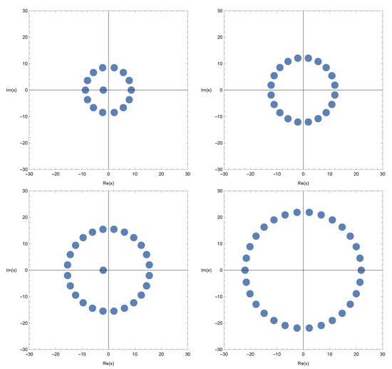
Figure 1. Stacking structure of approximation roots in $(p,q)$-cosine geometric polynomials when $n=15,20,25,30,p=\frac{1}{2},q=\frac{1}{10},y=3$ and $z=2$.

In Figure 1 (top-left), we took $n=15,p=\frac{1}{2},q=\frac{1}{10},y=3$ and $z=2$. In Figure 1 (top-right), we took $n=20,p=\frac{1}{2},q=\frac{1}{10},y=3$ and $z=2$. In Figure 1 (bottom-left), we took $n=25,p=\frac{1}{2},q=\frac{1}{10},y=3$ and $z=2$. In Figure 1 (bottom-right), we took $n=30,p=\frac{1}{2},q=\frac{1}{10}y=3,$ and $z=2$.

For $1\le n\le 30$, stacks of the roots of the polynomials ${\mathfrak{F}}_n^{\left(C\right)}\left(x,y;z:p,q\right)$, forming a 3D structure, are investigated below (Figure 2).

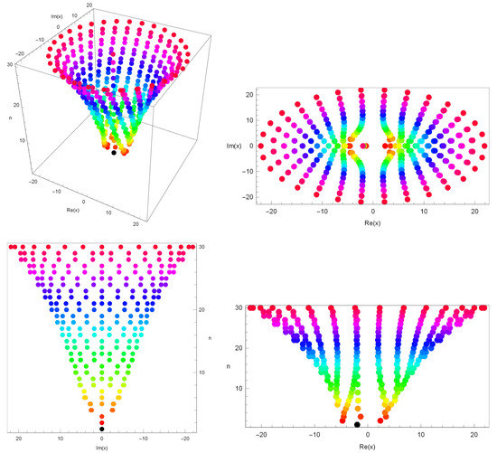
Figure 2. Stacking structure of approximation roots in $(p,q)$-cosine geometric polynomials when $1\le n\le 30,p=\frac{1}{2},q=\frac{1}{10},y=3$ and $z=2$ in 3D.

In Figure 2 (top-left), we drew stacks of roots of ${\mathfrak{F}}_n^{\left(C\right)}\left(x,y;z:p,q\right)=0$ for $1\le n\le 30$, $p=\frac{5}{10},q=\frac{1}{10}\mathrm{and}y=3,z=2$. In Figure 2 (top-right), we plotted x and y axes but no z axis in 3D. In Figure 2 (bottom-left), we drew y and z axes but no x axis in 3D. In Figure 2 (bottom-right), we drew x and z axes but no y axis in 3D.

Afterwards, we computed an approximate solution fulfilling ${\mathfrak{F}}_n^{\left(C\right)}\left(x,y;z:p,q\right)=0$. We provide some computations in Table 1.

Table 1. Approximate solutions of ${\mathfrak{F}}_n^{\left(C\right)}\left(x,3;2:\frac{1}{2},\frac{1}{10}\right)=0$.

Degree n	x
1	−2.0000
2	$-4.7553,2.3553$
3	$-4.5311,-1.3505,3.4017$
4	$-4.4787-2.6188i,-4.4787+2.6188i$,
	$3.2307-2.4655i,3.2307+2.4655i$,
5	$-4.1169-2.7012i,-4.1169+2.7012i$,
	$-1.8786,3.8066-2.8686,3.8066+2.8686i$
6	$-5.6938,-3.7903-4.1670i,-3.7903+4.1670i$,
	$3.1965-3.9149i,3.1965+3.9149i,4.3815$
7	$-5.5158,-3.5488-4.2483i,-3.5488+4.2483i$,
	$-1.8120,3.4186-4.2807i,3.4186+4.2807i$, 5.0883
8	$-5.9591-2.0319i,-5.9591+2.0319i,-3.2464-5.3214i$,
	$-3.2464+5.3214i,2.8252-5.1285i$,
	$2.8252+5.1285i,5.1303-1.9735i,5.1303+1.9735i$.

Plots of the real roots of ${\mathfrak{F}}_n^{\left(C\right)}\left(x,y;z:p,q\right)$ for $1\le n\le 30$ are shown in Figure 3.

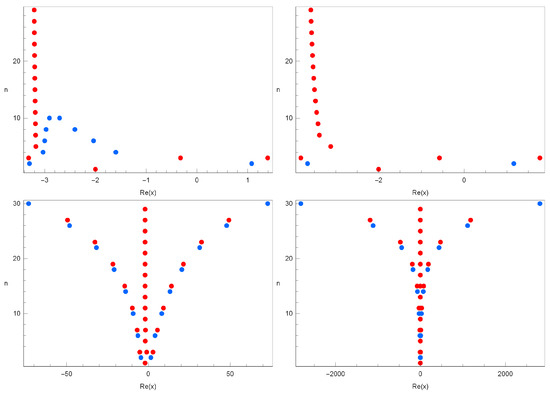
Figure 3. Stacking structure of approximation roots in $(p,q)$-cosine geometric polynomials when $1\le n\le 30,p=\frac{9}{10},\frac{8}{10},\frac{6}{10},\frac{5}{10},q=\frac{1}{10},\frac{2}{10},\frac{3}{10},\frac{4}{10},y=3$ and $z=2$.

In Figure 3 (top-left), we took $p=\frac{9}{10},q=\frac{1}{10},y=3,$ and $z=2$. In Figure 3 (top-right), we took $p=\frac{8}{10},q=\frac{2}{10},y=3,$ and $z=2$. In Figure 3 (bottom-left), we took $p=\frac{6}{10},q=\frac{3}{10},y=3$ and $z=2$. In Figure 3 (bottom-right), we took $p=\frac{5}{10},q=\frac{4}{10},y=3$ and $z=2$.

Next, certain zeros of the $(p,q)$-sine geometric polynomials and their graphical representations are shown.

A few of them are

$$\begin{array}{l}{\mathfrak{F}}_0^{\left(S\right)}\left(x,y;z:p,q\right)=0,\\ {\mathfrak{F}}_1^{\left(S\right)}\left(x,y;z:p,q\right)=y,\\ {\mathfrak{F}}_2^{\left(S\right)}\left(x,y;z:p,q\right)=2xy+2yz\\ {\mathfrak{F}}_3^{\left(S\right)}\left(x,y;z:p,q\right)={\displaystyle \frac{6p{x}^{2}y}{q+p}}-{\displaystyle \frac{6q^3{y}^3}{(q+p)(q^2+qp+p^2)}}+6xyz+6y\left({\displaystyle \frac{pz}{q+p}}+z^2\right)\\ {\mathfrak{F}}_4^{\left(S\right)}\left(x,y;z:p,q\right)={\displaystyle \frac{24p^3{x}^{3}y}{(q+p)(q^2+qp+p^2)}}-{\displaystyle \frac{24q^{3}x{y}^3}{(q+p)(q^2+qp+p^2)}}\\ +{\displaystyle \frac{24p{x}^{2}yz}{q+p}}-{\displaystyle \frac{24q^3{y}^{3}z}{(q+p)(q^2+qp+p^2)}}\\ +24xy\left({\displaystyle \frac{pz}{q+p}}+z^2\right)+24y\left({\displaystyle \frac{p^{3}z}{(q+p)(q^2+qp+p^2)}}+{\displaystyle \frac{2p{z}^2}{q+p}}+z^3\right).\end{array}$$

Now, we can develop the beautiful zeros of the polynomials ${\mathfrak{F}}_n^{\left(S\right)}\left(x,y;z:p,q\right)$ by making use of a math program on a computer. The roots of the polynomials ${\mathfrak{F}}_n^{\left(S\right)}\left(x,y;z:p,q\right)$ are illustrated in Figure 4.

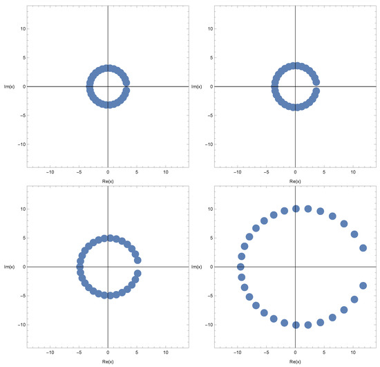
Figure 4. Stacking structure of approximation roots in $(p,q)$-sine geometric polynomials when $n=30,p=\frac{9}{10},\frac{8}{10},\frac{6}{10},\frac{5}{10},q=\frac{1}{10},\frac{2}{10},\frac{3}{10},\frac{4}{10},y=3$ and $z=2$.

In Figure 4 (top-left), we took $n=30,p=\frac{9}{10},q=\frac{1}{10},y=3$ and $z=2$. In Figure 4 (top-right), we took $n=30,p=\frac{8}{10},q=\frac{2}{10},y=3$ and $z=2$. In Figure 4 (bottom-left), we took $n=30,p=\frac{6}{10},q=\frac{3}{10},y=3$ and $z=2$. In Figure 4 (bottom-right), we took $n=30,p=\frac{5}{10},q=\frac{4}{10},y=3$ and $z=2$.

Stacks of roots of the polynomials ${\mathfrak{F}}_n^{\left(S\right)}\left(x,y;z:p,q\right)=0$ for $2\le n\le 30$, forming a three-dimensional structure, were developed and these are shown in Figure 5.

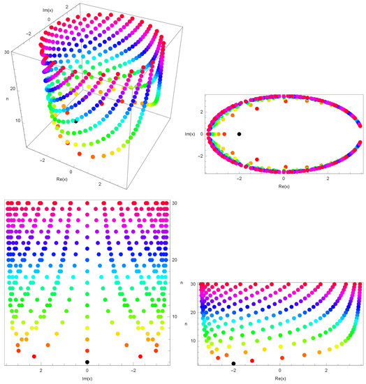
Figure 5. Stacking structure of approximation roots in $(p,q)$-sine geometric polynomials when $2\le n\le 30,p=\frac{1}{2},q=\frac{1}{10},y=3$ and $z=2$ in 3D.

In Figure 5 (top-left), we drew stacks of roots of ${\mathfrak{F}}_n^{\left(S\right)}\left(x,y;z:p,q\right)=0$ for $2\le n\le 30$, $p=\frac{5}{10},q=\frac{1}{10},y=3andz=2$. In Figure 5 (top-right), we drew x and y axes but no z axis in 3D. In Figure 5 (bottom-left), we drew y and z axes but no x axis in 3D. In Figure 5 (bottom-right), we drew x and z axes but no y axis in 3D.

Then, we computed an approximate solution fulfilling ${\mathfrak{F}}_n^{\left(S\right)}\left(x,y;z:p,q\right)=0$. We provide some computations in Table 2.

Table 2. Approximate solutions of ${\mathfrak{F}}_n^{\left(S\right)}\left(x,3;2:\frac{1}{2},\frac{1}{10}\right)=0$.

Degree n	x
2	−2.0000
3	$-1.2-2.30259i,-1.2+2.30259i$
4	$-2.67026,0.0951305-2.97641i,0.0951305+2.97641i$
5	$-2.30056-1.70626i,-2.30056+1.70626i$,
	$1.05256-3.0114i,1.05256+3.0114i$
6	$-2.93412,-1.48295-2.6397i$,
	$-1.48295+2.6397i,1.70041-2.84003i,1.70041+2.84003i$
7	$-2.72344-1.32366i,-2.72344+1.32366i,-0.666199-3.0794i$,
	$-0.666199+3.0794i,2.13972-2.61824i$, $2.13972+2.61824i$
8	$-3.07418,-2.19106-2.21365i$,
	$-2.19106+2.21365i,0.0333249-3.2403i$,
	$0.0333249+3.2403i,2.44484-2.39949i,2.44484+2.39949i$
9	$-2.93869-1.07528i,-2.93869+1.07528i$,
	$-1.57796-2.76974i,-1.57796+2.76974i,0.603827-3.25043i$,
	$0.603827+3.25043i,2.66283-2.20036i,2.66283+2.20036i$.

5. Conclusions

Utilizing $\left(p,q\right)$-numbers and $\left(p,q\right)$-concepts, Duran et al. [1] considered $\left(p,q\right)$-Genocchi polynomials and numbers, $\left(p,q\right)$-Bernoulli polynomials and numbers and $\left(p,q\right)$-Euler polynomials and numbers and provided many properties and formulas for these polynomials. Inspired and motivated by this consideration, many authors have introduced $(p,q)$-special numbers and polynomials and have described their several identities and properties. In this paper, using the $(p,q)$-cosine polynomials and $(p,q)$-sine polynomials, we have introduced novel kinds of $(p,q)$-extensions of geometric polynomials and have acquired multifarious properties and identities by making use of some series manipulation methods. Furthermore, we have computed the $\left(p,q\right)$-integral representations and $\left(p,q\right)$-derivative operator rules for these polynomials. Moreover, we have determined the approximate root movements of the new mentioned polynomials in a complex plane, utilizing the Newton method and illustrating them in figures. The structure of the approximate roots will come out in various ways, depending on the condition of the variables, and new methods and theorems related to this topic need to be created and proven.

Finally, we consider more general problems. How many roots do ${\mathfrak{F}}_n^{\left(C\right)}\left(x,y;z:p,q\right)$ = 0 and ${\mathfrak{F}}_n^{\left(S\right)}\left(x,y;z:p,q\right)=0$ have? We are not able to decide whether ${\mathfrak{F}}_n^{\left(C\right)}\left(x,y;z:p,q\right)=0$ and ${\mathfrak{F}}_n^{\left(S\right)}\left(x,y;z:p,q\right)=0$ have n distinct solutions. Here we leave a question: “Prove or disprove that ${\mathfrak{F}}_n^{\left(C\right)}\left(x,y;z:p,q\right)=0$ and ${\mathfrak{F}}_n^{\left(S\right)}\left(x,y;z:p,q\right)=0$ have n distinct solutions”. This question is an unsolved problem for all variables n (see Table 1 and Table 2). If we can theoretically prove the above problem by drawing new ideas from various numerical results, we look forward to contributing to research related to the roots of our new polynomials in applied mathematics, mathematical physics and engineering.

Not only can the ideas presented in this paper be utilized for similar polynomials, but these polynomials may also have possible applications in other scientific areas besides the applications described at the end of the paper. We would like to continue to study this line of research in the future.

References

- Duran, U.; Acikgoz, M.; Araci, S. On (p,q)-Bernoulli, (p,q)-Euler and (p,q)-Genocchi polynomials. J. Comput. Theor. Nanosci. 2016, 13, 7833–7908. [Google Scholar] [CrossRef]
- Khan, W.A.; Nisar, K.S.; Baleanu, D. A note on (p,q)-analogue type of Fubini numbers and polynomials. AIMS Math. 2020, 5, 2743–2757. [Google Scholar] [CrossRef]
- Njionou Sadjang, P. On (p, q)-Appell Polynomials. Anal. Math. 2019, 45, 583–598. [Google Scholar] [CrossRef]
- Sadjang, P.N.; Duran, U. On two bivariate kinds of (p,q)-Bernoulli polynomials. Miskolc. Math. Notes 2019, 20, 1185–1199. [Google Scholar] [CrossRef]
- Khan, W.A.; Khan, I.A.; Duran, U.; Acikgoz, M. Apostol type (p,q)-Frobenius Eulerian polynomials and numbers. Afr. Mat. 2021, 32, 115–130. [Google Scholar] [CrossRef]
- Duran, U.; Acikgoz, M. Apostol type (p,q)-Frobenious-Euler polynomials and numbers. Kragujev. J. Math. 2018, 42, 555–567. [Google Scholar] [CrossRef] [Green Version]
- Khan, W.A.; Muhiuddin, G.; Duran, U.; Al-Kadi, D. On (p,q)-sine and (p,q)-cosine Fubini polynomials. Symmetry 2022, 14, 527. [Google Scholar] [CrossRef]
- Ryoo, C.S.; Kang, J.Y. Explicit properties of q-cosine and q-sine Euler polynomials containing symmetric structures. Symmetry 2020, 12, 1247. [Google Scholar] [CrossRef]
- Gupta, V. (p,q)-Baskakov-Kontorovich operators. Appl. Math. Inf. Sci. 2016, 10, 1551–1556. [Google Scholar] [CrossRef]
- Jain, P.; Basu, C.; Panwar, V. On the (p,q)-Mellin transform and its applications. Acta Math. Sci. 2021, 4, 1719–1732. [Google Scholar] [CrossRef]
- Sadjang, P.N. On the fundamental theorem of (p,q)-calculus and some (p,q)-Taylor formulas. Res. Math. 2018, 73, 39. [Google Scholar] [CrossRef]
- Dil, A.; Kurt, V. Investigating geometric and exponential polynomials with Euler-Seidel matrices. J. Integer. Seq. 2011, 14, 1–12. [Google Scholar]
- Kargin, L. Some formulae for products of Fubini polynomials with applications. arXiv 2016, arXiv:1701.01023. [Google Scholar]
- Boyadzhiev, K.N. A series transformation formula and related polynomials. Int. J. Math. Math. Sci. 2005, 23, 3849–3866. [Google Scholar] [CrossRef] [Green Version]
- Tanny, S.M. On some numbers related to Bell numbers. Can. Math. Bull. 1974, 17, 733–738. [Google Scholar] [CrossRef]
- Jamei, M.-M.; Koepf, W. Symbolic computation of some power-trigonometric series. J. Symb. Comput. 2017, 80, 273–284. [Google Scholar] [CrossRef]
Publisher’s Note: MDPI stays neutral with regard to jurisdictional claims in published maps and institutional affiliations. |
© 2022 by the authors. Licensee MDPI, Basel, Switzerland. This article is an open access article distributed under the terms and conditions of the Creative Commons Attribution (CC BY) license (https://creativecommons.org/licenses/by/4.0/).