Analytic Valuation Formula for American Strangle Option in the Mean-Reversion Environment

Abstract

This paper investigates the American strangle option in a mean-reversion environment. When the underlying asset follows a mean-reverting lognormal process, an analytic pricing formula for an American strangle option is explicitly provided. To present the pricing formula, we consider the partial differential equation (PDE) for American strangle options with two optimal stopping boundaries and use Mellin transform techniques to derive the integral equation representation formula arising from the PDE. A Monte Carlo simulation is used as a benchmark to validate the formula’s accuracy and efficiency. In addition, the numerical examples are provided to demonstrate the effects of the mean-reversion on option prices and the characteristics of options with respect to several significant parameters.

1. Introduction

The Black–Scholes model, which was proposed in 1973, has provided the theoretical base for the pricing of options in financial market [1]. Under the Black–Scholes model, various option pricing problems, including European and American options, have been extensively studied over the last few decades. We investigate the American style option-pricing problem in this paper. In fact, while a European options has a closed-form pricing formula, an American option does not. This is because, unlike a European option, an American option is a contract that allows holders to exercise at any time before the maturity. Because of this feature, the American option-pricing problem can be represented as a free-boundary problem. To obtain the boundary and price of the American option, numerical methods have been mainly used based on classic methods such as tree methods [2,3,4], finite difference methods [5,6], analytical approximation methods [7,8], integral representation methods [9,10], and Monte Carlo simulation methods [11,12].

In recent years, many researchers have proposed exotic American style options with various approaches. Based on the Laplace–Carson Transform (LCT) approach, Park and Jeon [13] and Kang et al. [14] obtained numerically the prices of American knock-out options with rebate and American strangle options, respectively. Zaevski [15] proposed a new form of the early exercise premium for the American type options using the technique of stopping times. Lee [16] investigated the American power options and provided an efficient numerical method for pricing the options. In Deng [17], the valuation of perpetual American floating-strike option under stochastic volatility was considered using a multiscale asymptotic technique. Qui [18] studied a system of two nonlinear integral equations arising from the early exercise premium representation for an American strangle option under the Black–Scholes model. Zaevski [19] developed the early exercise boundary for American derivatives with a new approach that imposed continuity on the exponent of piecewise linear functions. More recently, in Jeon and Kim [20], the integral equation representation for American better-of option with two underlying assets was derived using Mellin transform methods. The discounted American capped options were studied in Zaevski [21]. In this paper, we also study the extension of American style options. Specifically, we consider American strangle options with two optimal boundaries in a mean-reversion environment.

Mean-reverting models, which describe a mean-reversion environment, have been widely used to price various financial derivatives. Through the dynamics of the domestic and foreign term structure of interest rates, Sorensen [22] proposed a mean-reverting process for currency exchange rates. Sorensen found that the mean-reverting feature has an effect on plain vanilla currency option prices [22]. Hui and Lo [23] adopted a mean-reverting lognormal (MRL) model to investigate the pricing behavior of options with a barrier, which is a deterministic function of time designed to match the coefficients of the governing partial different equation for the barrier option. Hui and Lo found that the parameters in the MRL model had a significant impact on the valuation and hedging parameters of barrier options [23]. Wong and Lau [24] studied exotic path-dependent options and provided an efficient and accurate approach for valuing the options under the MRL model. Motivated by these works and the work of Kang et al. [14], we consider the MRL model for the underlying asset as an extensional work for the American strangle option pricing. We used the partial differential equation (PDE) approach to present the pricing formula of the American strangle option under the MRL model explicitly. Several studies have been conducted to deal with PDE for American style options using Mellin transform techniques [25,26,27,28]. We also develop Mellin transform techniques for the PDE of an American type option. More specifically, we derive the integral equation representation for the price of American strangle option when the underlying asset follows the MRL model.

The remainder of this paper is structured as follows. In Section 2, we propose a mean-reverting lognormal model for a mean-reversion environment and formulate the problem addressed in this paper. In Section 3, we demonstrate the analytical pricing formula for the American strangle option under the proposed model. In Section 4, we provide some numerical experiments. In Section 5, we present concluding remarks.

2. Model

Under the mean-reversion environment, we investigate the American strangle option with the finite maturity $T>0$, which consists of a call option with strike price $K_1>0$ and a put option with strike price $K_2>0$, That is, we assume that the underlying asset $S_t$ has the following dynamics, under risk-neutral measure $\mathbb{Q}$:

$${\displaystyle \frac{d{S}_t}{S_t}}=\kappa (\mu -log{S}_t)dt+\sigma d{B}_t,$$

(1)

where $\kappa$ is the speed of reversion, $\sigma >0$ is the volatility of the underlying asset, and $\mu$ represents the equilibrium mean level of the asset. Here, we assume that the parameters $\kappa$, $\sigma$, and $\mu$ are constants. ${(B_t)}_{t=0}^T$ is a one-dimensional standard Brownian motion defined on the probability space $(\mathrm{\Omega },\mathcal{F},\mathbb{Q})$, where ${({\mathcal{F}}_t)}_{t=0}^T$ is the natural filtration generated by ${(B_t)}_{t=0}^T$.

Remark 1.

In Hui and Lo [23] and Wang and Lau [24], they assumed that the risk-neutral dynamic of the exchange rate (i.e., the domestic currency value of a unit of foreign currency) followed the mean-reverting lognormal process as in (1).

We assume that

$$K_1>K_2.$$

Let $V(t,S_t)$ be the price of an American strangle option at time $t\in [0,T]$. In the absence of arbitrage opportunities, $V(t,S_t)$ is expressed as the following optimal stopping problem:

Problem 1

(American strangle).

$$\begin{array}{c}\hfill V(t,S_t)=\underset{\tau \in \mathcal{U}(t,T)}{sup}{\mathbb{E}}^{\mathbb{Q}}\left[e^{-r(\tau -t)}\left({(S_{\tau }-K_1)}^{+}+{(K_2-S_{\tau })}^{+}\right)\mid {\mathcal{F}}_t\right],\end{array}$$

(2)

where ${\mathbb{E}}^{\mathbb{Q}}$ is the expectation with respect to the probability measure $\mathbb{Q}$, $r>0$ is the constant risk-free interest rate, $\mathcal{U}(t,T)$ is the set of all ${\mathcal{F}}_t$-stopping times taking values in $[t,T]$, and ${(a)}^{+}:=max\{a,0\}$.

3. Analytic Representation for American Strangle Options

According to a standard theory of optimal stopping problem, the value $V(t,s)$ satisfies the following variational inequality arising from Problem 1: on the domain ${\mathcal{D}}_T:=\{(t,s)\mid 0\le t<T,0<s<\infty \}$

$$\begin{array}{c}\hfill \left\{\begin{array}{c}{\partial }_{t}V+\mathcal{L}V\le 0\mathrm{for}V(t,s)={(s-K_1)}^{+}+{(K_2-s)}^{+},\hfill \\ {\partial }_{t}V+\mathcal{L}V=0\mathrm{for}V(t,s)>{(s-K_1)}^{+}+{(K_2-s)}^{+},\hfill \\ V(T,s)={(s-K_1)}^{+}+{(K_2-s)}^{+},\hfill \end{array}\right.\end{array}$$

(3)

where the differential operator $\mathcal{L}$ is given by

$$\mathcal{L}:=s^2{\partial }_{ss}+\kappa (\mu -logs)s{\partial }_s-r.$$

We define the waiting and stopping region $\mathbf{WR}$ and $\mathbf{SR}$ as follows:

$$\begin{array}{cc}\hfill \mathbf{WR}& :=\{(t,s)\in {\mathcal{D}}_T\mid V(t,s)>{(s-K_1)}^{+}+{(K_2-s)}^{+}\},\hfill \\ \hfill \mathbf{SR}& :=\{(t,s)\in {\mathcal{D}}_T\mid V(t,s)={(s-K_1)}^{+}+{(K_2-s)}^{+}\}.\hfill \end{array}$$

(4)

Moreover, the stopping region $\mathbf{SR}$ can be divided into the following two subregions:

$$\begin{array}{c}\hfill {\mathbf{SR}}_{\mathrm{up}}:=\{(t,s)\in \mathbf{SR}\mid V(t,s)={(s-K_1)}^{+}\}\mathrm{and}{\mathbf{SR}}_{\mathrm{low}}:=\{(t,s)\in \mathbf{SR}\mid V(t,s)={(K_2-s)}^{+}\}.\end{array}$$

(5)

That is,

$$\mathbf{SR}={\mathbf{SR}}_{\mathrm{up}}\cup {\mathbf{SR}}_{\mathrm{low}}\mathrm{and}{\mathbf{SR}}_{\mathrm{up}}\cap {\mathbf{SR}}_{\mathrm{low}}=\varnothing .$$

Since the value $V(t,s)$ should be positive when the option holder exercises early, we can rewrite the two regions ${\mathbf{SR}}_{\mathrm{up}}$ and ${\mathbf{SR}}_{\mathrm{low}}$ as follows:

$$\begin{array}{c}\hfill {\mathbf{SR}}_{\mathrm{up}}=\{(t,s)\in \mathbf{SR}\mid V(t,s)=s-K_1\}\mathrm{and}{\mathbf{SR}}_{\mathrm{low}}=\{(t,s)\in \mathbf{SR}\mid V(t,s)=K_2-s\}.\end{array}$$

(6)

Then, there exist two optimal exercise boundaries ${\mathcal{Z}}_{\mathrm{up}}(t)$ and ${\mathcal{Z}}_{\mathrm{low}}(t)$ defined as

$$\begin{array}{c}\hfill {\mathcal{Z}}_{\mathrm{up}}(t)=sup\{s>0\mid (t,s)\in \mathbf{WR}\}\mathrm{and}{\mathcal{Z}}_{\mathrm{low}}(t)=inf\{s>0\mid (t,s)\in \mathbf{WR}\}.\end{array}$$

In terms of the two boundaries ${\mathcal{Z}}_{\mathrm{up}}(t)$ and ${\mathcal{Z}}_{\mathrm{low}}(t)$,

$$\begin{array}{c}\hfill {\mathbf{SR}}_{\mathrm{up}}=\{(t,s)\in \mathbf{SR}\mid s\ge {\mathcal{Z}}_{\mathrm{up}}(t)\}\mathrm{and}{\mathbf{SR}}_{\mathrm{low}}=\{(t,s)\in \mathbf{SR}\mid 0<s\le {\mathcal{Z}}_{\mathrm{low}}(t)\}.\end{array}$$

(7)

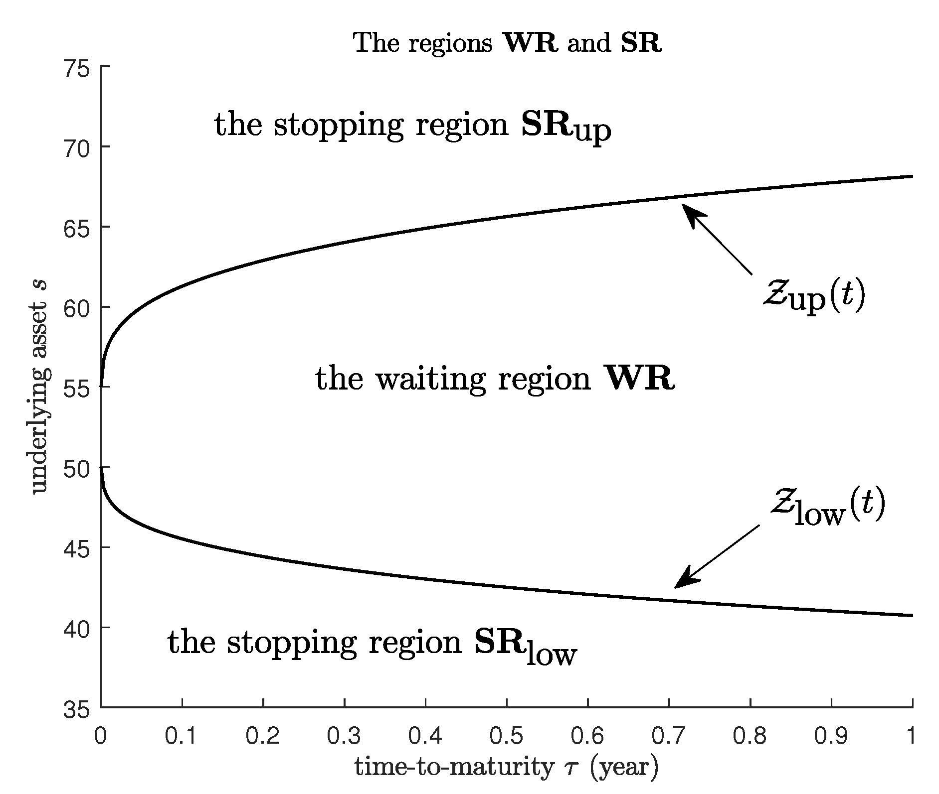
Figure 1 illustrates the regions with the boundaries. At the boundaries $s={\mathcal{Z}}_{\mathrm{up}}(t)$ or $s={\mathcal{Z}}_{\mathrm{low}}(t)$, the following smooth-pasting condition (or supercontact) holds:

$$\begin{array}{c}\hfill \left\{\begin{array}{c}V(t,{\mathcal{Z}}_{\mathrm{up}}(t))={\mathcal{Z}}_{\mathrm{up}}(t)-K_1,{\partial }_{s}V(t,{\mathcal{Z}}_{\mathrm{up}}(t))=1,\hfill \\ V(t,{\mathcal{Z}}_{\mathrm{low}}(t))=K_2-{\mathcal{Z}}_{\mathrm{low}}(t),{\partial }_{s}V(t,{\mathcal{Z}}_{\mathrm{low}}(t))=-1.\hfill \end{array}\right.\end{array}$$

(8)

Figure 1. The waiting region $\mathbf{WR}$, the stopping region $\mathbf{SR}$, the two free boundaries ${\mathcal{Z}}_{\mathrm{up}}(t)$, and ${\mathcal{Z}}_{\mathrm{low}}(t)$.

Since $V(t,s)=s-K_1$ for $s\ge {\mathcal{Z}}_{\mathrm{up}}(t)$ and $V(t,s)=K_2-s$ for $0<s\le {\mathcal{Z}}_{\mathrm{low}}(t)$, we deduce that $V(t,s)$ satisfies the following nonhomogeneous PDE:

$$\begin{array}{c}\hfill {\partial }_{t}V+\mathcal{L}V=\left((r{K}_1+(\kappa \mu -r-\kappa logs)s){\mathbf{1}}_{\{s\ge {\mathcal{Z}}_{\mathrm{up}}(t)\}}+(-r{K}_2-(\kappa \mu -r-\kappa logs)s)\right){\mathbf{1}}_{\{0<s\le {\mathcal{Z}}_{\mathrm{low}}(t)\}}\end{array}$$

(9)

with the terminal condition $V(T,s)={(s-K_1)}^{+}+{(K_2-s)}^{+}$ and the smooth-pasting condition (8).

By applying the Mellin transform to the nonhomogeneous PDE (9), we derive the integral equation representation formula for $V(t,s)$ using the results in Appendix A.

Theorem 1.

The price $V(t,s)$ of the American strangle option defined in Problem 1 is represented as

$$\begin{array}{c}\hfill V(t,s)=C_E(t,s)+P_E(t,s)+V_{ep}(t,s)\end{array}$$

(10)

where $C_E$ and $P_E$ are the price of European call and put options, respectively, and $V_{ep}$ is the early exercise premium for the American strangle option:

$$\begin{array}{cc}\hfill C_E(t,s)=& e^{-r\tau +\theta (1-e^{-\tau \tau })+\frac{1}{2}{(\alpha (\tau ))}^2}{s}^{e^{-\kappa \tau }}\mathcal{N}\left(d_1(\tau ,\frac{s}{K_1})\right)-K_1{e}^{-\rho \tau }\mathcal{N}\left(d_2(\tau ,\frac{s}{K_1})\right),\hfill \\ \hfill P_E(t,s)=& K_2{e}^{-\rho \tau }\mathcal{N}\left(-d_2(\tau ,\frac{s}{K_2})\right)-e^{-r\tau +\theta (1-e^{-\tau \tau })+\frac{1}{2}{(\alpha (\tau ))}^2}{s}^{e^{-\kappa \tau }}\mathcal{N}\left(-d_1(\tau ,\frac{s}{K_2})\right)\hfill \end{array}$$

and

$$\begin{array}{cc}\hfill & V_{ep}(t,s)\hfill \\ \hfill =& {\int }_0^{\tau }{e}^{-r\xi +\theta (1-e^{-\kappa \xi })+\frac{1}{2}a{(\xi )}^2}{s}^{e^{-\kappa \xi }}\left\{\left[(r-\kappa \mu )+\kappa (e^{-\kappa \xi }logs+\theta (1-e^{-\kappa \xi })+{(a(\xi ))}^2)\right]\right.\hfill \\ \hfill \times & \left.\mathcal{N}\left(d_1(\xi ,{\displaystyle \frac{s}{{\mathcal{Z}}_{\mathrm{up}}(t+\xi )}})\right)+\kappa a(\xi )\mathbf{n}\left(d_1(\xi ,{\displaystyle \frac{s}{{\mathcal{Z}}_{\mathrm{up}}(t+\xi )}})\right)\right\}d\xi -r{K}_1{\int }_0^{\tau }{e}^{-r\xi }\mathcal{N}\left(d_2(\xi ,\frac{s}{{\mathcal{Z}}_{\mathrm{up}}(t+\xi )})\right)d\xi \hfill \\ \hfill -& {\int }_0^{\tau }{e}^{-r\xi +\theta (1-e^{-\kappa \xi })+\frac{1}{2}a{(\xi )}^2}{s}^{e^{-\kappa \xi }}\left\{\left[(r-\kappa \mu )+\kappa (e^{-\kappa \xi }logs+\theta (1-e^{-\kappa \xi })+{(a(\xi ))}^2)\right]\right.\hfill \\ \hfill \times & \left.\mathcal{N}\left(-d_1(\xi ,{\displaystyle \frac{s}{{\mathcal{Z}}_{\mathrm{low}}(t+\xi )}})\right)-\kappa a(\xi )\mathbf{n}\left(d_1(\xi ,{\displaystyle \frac{s}{{\mathcal{Z}}_{\mathrm{low}}(t+\xi )}})\right)\right\}d\xi +r{K}_2{\int }_0^{\tau }{e}^{-r\xi }\mathcal{N}\left(-d_2(\xi ,\frac{s}{{\mathcal{Z}}_{\mathrm{low}}(t+\xi )})\right)d\xi ,\hfill \end{array}$$

where $\mathcal{N}(·)$ and $\mathbf{n}(·)$ are the standard normal cumulative distribution and probability functions, respectively, $\tau =T-t$,

$$\begin{array}{c}\hfill a(t):=\sigma {\left({\displaystyle \frac{1-e^{-2\kappa t}}{2\kappa }}\right)}^{\frac{1}{2}},d_1(t,s):={\displaystyle \frac{e^{-\kappa t}logs+\theta (1-e^{-\kappa t})+{(a(t))}^2}{a(t)}},d_2(t,s)=d_1(t,s)-a(t),\end{array}$$

and

$$\theta :=\mu -{\displaystyle \frac{{\sigma }^2}{2\kappa }}.$$

Moreover, the two free boundaries ${\mathcal{Z}}_{\mathrm{up}}(t)$ and ${\mathcal{Z}}_{\mathrm{low}}(t)$ satisfy the following coupled integral equations:

$$\begin{array}{c}\hfill \left\{\begin{array}{c}{\mathcal{Z}}_{\mathrm{up}}(t)-K_1=V_{ep}(t,{\mathcal{Z}}_{\mathrm{up}}(t)),\hfill \\ K_2-{\mathcal{Z}}_{\mathrm{low}}(t)=V_{ep}(t,{\mathcal{Z}}_{\mathrm{low}}(t)).\hfill \end{array}\right.\end{array}$$

(11)

Proof. 

Recall that $V(t,s)$ satisfies

$$\begin{array}{cc}\hfill & {\partial }_{t}V+\mathcal{L}V=\left((r{K}_1+(\kappa \mu -r-\kappa logs)s){\mathbf{1}}_{\{s\ge {\mathcal{Z}}_{\mathrm{up}}(t)\}}+(-r{K}_2-(\kappa \mu -r-\kappa logs)s)\right){\mathbf{1}}_{\{0<s\le {\mathcal{Z}}_{\mathrm{low}}(t)\}},\hfill \end{array}$$

(12)

with $V(T,s)={(s-K_1)}^{+}+{(K_2-s)}^{+}$.

By applying the result (A13) in Appendix A with $W(t,s)=V(t,s)$, $h(s)={(s-K_1)}^{+}+{(K_2-s)}^{+}$ and

$$f(t,s)=\left((r{K}_1+(\kappa \mu -r-\kappa logs)s){\mathbf{1}}_{\{s\ge {\mathcal{Z}}_{\mathrm{up}}(t)\}}+(-r{K}_2-(\kappa \mu -r-\kappa logs)s)\right){\mathbf{1}}_{\{0<s\le {\mathcal{Z}}_{\mathrm{low}}(t)\}},$$

we have

$$\begin{array}{c}\hfill V(t,s)=C_E(t,s)+P_E(t,s)+V_{ep}(t,s),\end{array}$$

where

$$\begin{array}{c}\hfill C_E(t,s)={\int }_{K_1}^{\infty }{e}^{-\kappa \tau }\left(u^{e^{-\kappa \tau }}-K_1\right)\mathrm{\Xi }(t,\frac{s}{u}){\displaystyle \frac{du}{u}},P_E(t,s)={\int }_0^{K_2}{e}^{-\kappa \tau }\left(K_2-u^{e^{-\kappa \tau }}\right)\mathrm{\Xi }(t,\frac{s}{u}){\displaystyle \frac{du}{u}},\end{array}$$

and

$$\begin{array}{cc}\hfill V_{ep}(t,s)=& {\int }_0^{\tau }\left\{{\int }_{{\mathcal{Z}}_{\mathrm{up}}(t+\xi )}^{\infty }\left(r{K}_1+(\kappa \mu -r-\kappa logu)u\right)\mathrm{\Xi }(\xi ,{\displaystyle \frac{s}{u}}){\displaystyle \frac{du}{u}}\right\}d\xi \hfill \\ \hfill +& {\int }_0^{\tau }\left\{{\int }_0^{{\mathcal{Z}}_{\mathrm{low}}(t+\xi )}\left(-r{K}_2-(\kappa \mu -r-\kappa logu)u\right)\mathrm{\Xi }(\xi ,{\displaystyle \frac{s}{u}}){\displaystyle \frac{du}{u}}\right\}d\xi .\hfill \end{array}$$

By applying Lemma A1 in Appendix A to above the integral representations for $C_E$, $P_E$, and $V_{ep}$, we can derive the desired result. □

Remark 2.

Let us consider the following generalized American strangle option in a mean-reversion environment:

$$V_{p,q}(t,S_t)=\underset{\tau \in \mathcal{U}(t,T)}{sup}{\mathbb{E}}^{\mathbb{Q}}\left[e^{-r(\tau -t)}\left(p{(S_{\tau }-K_1)}^{+}+q{(K_2-S_{\tau })}^{+}\right)\mid {\mathcal{F}}_t\right].$$

(13)

As in Theorem 1, we can easily obtain

$$V_{p,q}(t,s)=p{C}_E(t,s)+q{P}_E(t,s)+V_{ep}^{p,q}(t,s),$$

(14)

where

$$\begin{array}{cc}\hfill & V_{ep}^{p,q}(t,s)\hfill \\ \hfill =& p\left[{\int }_0^{\tau }{e}^{-r\xi +\theta (1-e^{-\kappa \xi })+\frac{1}{2}a{(\xi )}^2}{s}^{e^{-\kappa \xi }}\left\{\left[(r-\kappa \mu )+\kappa (e^{-\kappa \xi }logs+\theta (1-e^{-\kappa \xi })+{(a(\xi ))}^2)\right]\right.\right.\hfill \\ \hfill \times & \left.\left.\mathcal{N}\left(d_1(\xi ,{\displaystyle \frac{s}{{\mathcal{Z}}_{\mathrm{up}}^{p,q}(t+\xi )}})\right)+\kappa a(\xi )\mathbf{n}\left(d_1(\xi ,{\displaystyle \frac{s}{{\mathcal{Z}}_{\mathrm{up}}^{p,q}(t+\xi )}})\right)\right\}d\xi -r{K}_1{\int }_0^{\tau }{e}^{-r\xi }\mathcal{N}\left(d_2(\xi ,\frac{s}{{\mathcal{Z}}_{\mathrm{up}}^{p,q}(t+\xi )})\right)d\xi \right]\hfill \\ \hfill -& q\left[{\int }_0^{\tau }{e}^{-r\xi +\theta (1-e^{-\kappa \xi })+\frac{1}{2}a{(\xi )}^2}{s}^{e^{-\kappa \xi }}\left\{\left[(r-\kappa \mu )+\kappa (e^{-\kappa \xi }logs+\theta (1-e^{-\kappa \xi })+{(a(\xi ))}^2)\right]\right.\right.\hfill \\ \hfill \times & \left.\left.\mathcal{N}\left(-d_1(\xi ,{\displaystyle \frac{s}{{\mathcal{Z}}_{\mathrm{low}}^{p,q}(t+\xi )}})\right)-\kappa a(\xi )\mathbf{n}\left(d_1(\xi ,{\displaystyle \frac{s}{{\mathcal{Z}}_{\mathrm{low}}^{p,q}(t+\xi )}})\right)\right\}d\xi +r{K}_2{\int }_0^{\tau }{e}^{-r\xi }\mathcal{N}\left(-d_2(\xi ,\frac{s}{{\mathcal{Z}}_{\mathrm{low}}^{p,q}(t+\xi )})\right)d\xi \right].\hfill \end{array}$$

Moreover, the two free boundaries ${\mathcal{Z}}_{\mathrm{up}}^{p,q}(t)$ and ${\mathcal{Z}}_{\mathrm{low}}^{p,q}(t)$ satisfy the following coupled integral equations:

$$\begin{array}{c}\hfill \left\{\begin{array}{c}p({\mathcal{Z}}_{\mathrm{up}}^{p,q}(t)-K_1)=V_{ep}^{p,q}(t,{\mathcal{Z}}_{\mathrm{up}}^{p,q}(t)),\hfill \\ q(K_2-{\mathcal{Z}}_{\mathrm{low}}^{p,q}(t))=V_{ep}^{p,q}(t,{\mathcal{Z}}_{\mathrm{low}}^{p,q}(t)).\hfill \end{array}\right.\end{array}$$

(15)

Remark 3.

Using the result in Theorem 1, the integral equation representations for the free-boundary and option value of an American call $V_C(t,s)$ and put $V_P(t,s)$ are derived in the mean-reversion environment. For more details on the derivation, see Appendix B.

Proposition 1.

The following limits holds:

$$\underset{t\to T-}{lim}{\mathcal{Z}}_{\mathrm{up}}(t)=max\left\{K_1,\overline{z}\right\}and\underset{t\to T-}{lim}{\mathcal{Z}}_{\mathrm{low}}(t)=min\left\{K_2,\underline{z}\right\},$$

where $\overline{z}$ and $\underline{z}$ solve the following algebraic equations

$$r{K}_1-(r-\kappa \mu +\kappa log\overline{z})\overline{z}=0andr{K}_2-(r-\kappa \mu +\kappa log\underline{z})\underline{z}=0,$$

respectively.

Proof. 

Suppose that ${\mathcal{Z}}_{\mathrm{up}}(\theta )<K_1$ for some $t\in [0,T)$. Then, the early exercise profit ${\mathcal{Z}}_{\mathrm{up}}(t)-K_1$ becomes negative. However, the early exercise privilege cannot be a liability so that we can rule out the possibility ${\mathcal{Z}}_{\mathrm{up}}(t)<K_1$. That is, ${\mathcal{Z}}_{\mathrm{up}}(t)\ge K_1$ for all $\tau \in [0,T)$. Thus, we have ${\mathcal{Z}}_{\mathrm{up}}(T-)\ge K_1$.

Since $\mathbf{SR}={\mathbf{SR}}_{\mathrm{up}}\cup {\mathbf{SR}}_{\mathrm{low}}$, the variational inequality (3) implies that

$${\partial }_{t}V+\mathcal{L}V\le 0\mathrm{for}(t,s)\in {\mathbf{SR}}_{\mathrm{up}}.$$

(16)

It follows from $V(t,s)=s-K_1$ in ${\mathbf{SR}}_{\mathrm{up}}$ that

$$r{K}_1-(r-\kappa \mu +\kappa logs)s\le 0in{\mathbf{SR}}_{\mathrm{up}}.$$

This implies that

$${\mathcal{Z}}_{\mathrm{up}}(T-)\ge max\{K_1,\overline{z}\},$$

where $\overline{z}$ solves $r{K}_1-(r-\kappa \mu +\kappa log\overline{z})\overline{z}=0$.

If ${\mathcal{Z}}_{\mathrm{up}}(T-)>max\{K_1,\overline{z}\}$, then there exists a domain ${\mathcal{D}}_{ϵ}$: $=\{(t,s)\mid T-ϵ\le t\le T,max\{K_1,\overline{z}\}<s<{\mathcal{Z}}_{\mathrm{up}}(T-)\}\subset \mathbf{WR}$ for a sufficiently small $ϵ>0$ such that

$${\partial }_{t}V+\mathcal{L}V=0\mathrm{for}(t,s)\in {\mathcal{D}}_{ϵ}.$$

At $t=T$ in the domain ${\mathcal{D}}_{ϵ}$, we deduce that

$${\partial }_{t}V{|}_{t=T}=-{\left[\mathcal{L}V(t,s)\right]}_{t=T}>0,$$

where we have used the fact that $V(T,s)=s-K_1$ for $(T,s)\in {\mathcal{D}}_{ϵ}$.

It follows that

$$V(t,s)<V(T,s)=s-K_1={(s-K_1)}^{+}\mathrm{in}{\mathcal{D}}_{ϵ},$$

which contradicts $V(t,s)>{(s-K_1)}^{+}$ in the domain ${\mathcal{D}}_{ϵ}\in \mathbf{WR}$.

Hence,

$${\mathcal{Z}}_{\mathrm{up}}(T-)=\underset{t\to T-}{lim}{\mathcal{Z}}_{\mathrm{up}}(t)=max\{K_1,\overline{z}\}.$$

By the almost similar argument, we derive that

$${\mathcal{Z}}_{\mathrm{low}}(T-)=min\{K_2,\underline{z}\},$$

where $\underline{z}$ solves $r{K}_2-(r-\kappa \mu +log\underline{z})\underline{z}=0$. □

4. Numerical Results

In this section, we carry out some numerical experiments for the prices of the American strangle option in the proposed model. We defined some default parameters for the numerical experiments. The following were the default parameter values.

$$S_0=55,T=1,\mu =4,r=0.03,\sigma =0.2,\kappa =0.5,K_1=55,\mathrm{and}{K}_2=50.$$

By utilizing the recursive integration method (RIM) proposed by Huang et al. [29], we can obtain the numerical solution for the coupled integral equation of ${\mathcal{Z}}_{\mathrm{up}}(t)$ and ${\mathcal{Z}}_{\mathrm{low}}(t)$ in Theorem 1. The detailed procedures for the numerical algorithm to solve the coupled integral equation are well documented in [30,31]. All experiments were implemented using Matlab on a personal computer with Intel(R) Core(TM) i7-6700 CPU.

We first demonstrated the accuracy and efficiency of our formula by comparing the option values obtained through the Monte Carlo (MC) simulation method. The time period $[0,T]$ was discretized into n time steps of equal length $T/n$, and the sample path was generated using the Euler–Maruyama discretization method to obtain the values using the MC simulation method. For all MC simulations, the number of sample paths was set to be 100,000, and the number of time steps was set to be 500. Table 1 presents the results of the numerical experiments with default parameters.

Table 1. Values and CPU times for RIM method and the MC simulation. CPU times are in seconds, and RE is defined by |RIM − MC|/MC × 100%.

			$\mathit{\mu }=2$			$\mathit{\mu }=4$
${\mathit{S}}_0$	r	$\mathit{\kappa }$	RIM	MC	Relative Error (RE)	RIM	MC	Relative Error (RE)
50	0.01	0.3	19.418	19.369	0.25%	5.474	5.434	0.74%
		0.5	26.245	26.220	0.17%	5.215	5.186	0.54%
		0.7	30.665	30.677	0.04%	5.029	5.002	0.53%
	0.03	0.3	19.034	19.004	0.16%	5.401	5.354	0.87%
		0.5	25.726	25.755	0.11%	5.149	5.166	0.83%
		0.7	30.058	30.088	0.10%	4.968	4.938	0.61%
	0.05	0.3	18.657	18.688	0.17%	5.329	5.279	0.94%
		0.5	25.216	25.234	0.07%	5.084	5.044	0.81%
		0.7	29.462	29.465	0.01%	4.909	4.872	0.72%
55	0.01	0.3	17.247	17.183	0.37%	5.876	5.821	0.95%
		0.5	24.862	24.819	0.17%	5.598	5.566	0.57%
		0.7	29.752	29.728	0.08%	5.382	5.771	0.21%
	0.03	0.3	16.907	16.810	0.58%	5.797	5.743	0.94%
		0.5	24.369	24.314	0.23%	5.526	5.505	0.37%
		0.7	29.163	29.168	0.02%	5.317	5.338	0.39%
	0.05	0.3	16.573	16.502	0.43%	5.719	5.680	0.69%
		0.5	23.887	23.847	0.17%	5.455	5.438	0.31%
		0.7	28.585	28.594	0.03%	5.525	5.228	0.46%
60	0.01	0.3	15.262	15.128	0.89%	7.639	7.604	0.46%
		0.5	23.526	23.603	0.33%	7.304	7.348	0.60%
		0.7	28.879	28.865	0.05%	7.063	7.055	0.10%
	0.03	0.3	14.966	14.829	0.92%	7.561	7.567	0.07%
		0.5	23.060	23.069	0.04%	7.239	7.248	0.12%
		0.7	28.307	28.329	0.07%	7.008	7.062	0.76%
	0.05	0.3	14.676	14.534	0.98%	7.486	7.505	0.26%
		0.5	22.603	22.632	0.12%	7.177	7.216	0.53%
		0.7	27.747	27.755	0.03%	6.954	6.953	0.02%
Av. run time (s)			RIM	0.016		MC	18.672

The option prices calculated by the formula in Theorem 1 using the RIM method are compared to the values obtained by the MC simulation method in Table 1. Table 1 also shows that the relative error (RE) between the option prices calculated using the RIM method and those calculated using the MC simulation is less than 1% in all cases. Moreover, our approach (RIM) took 0.016 s of CPU time on average to obtain a single option price, whereas the MC simulation took 18.672 s of CPU time on average to obtain a single option price. As a result, we conclude that our approach based on RIM method is accurate and efficient.

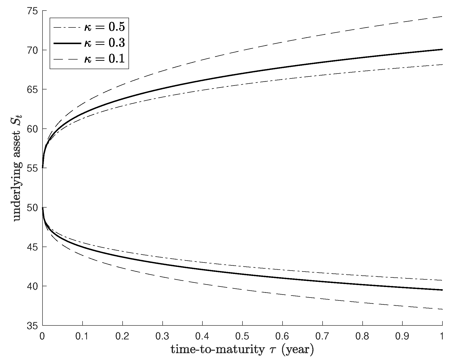
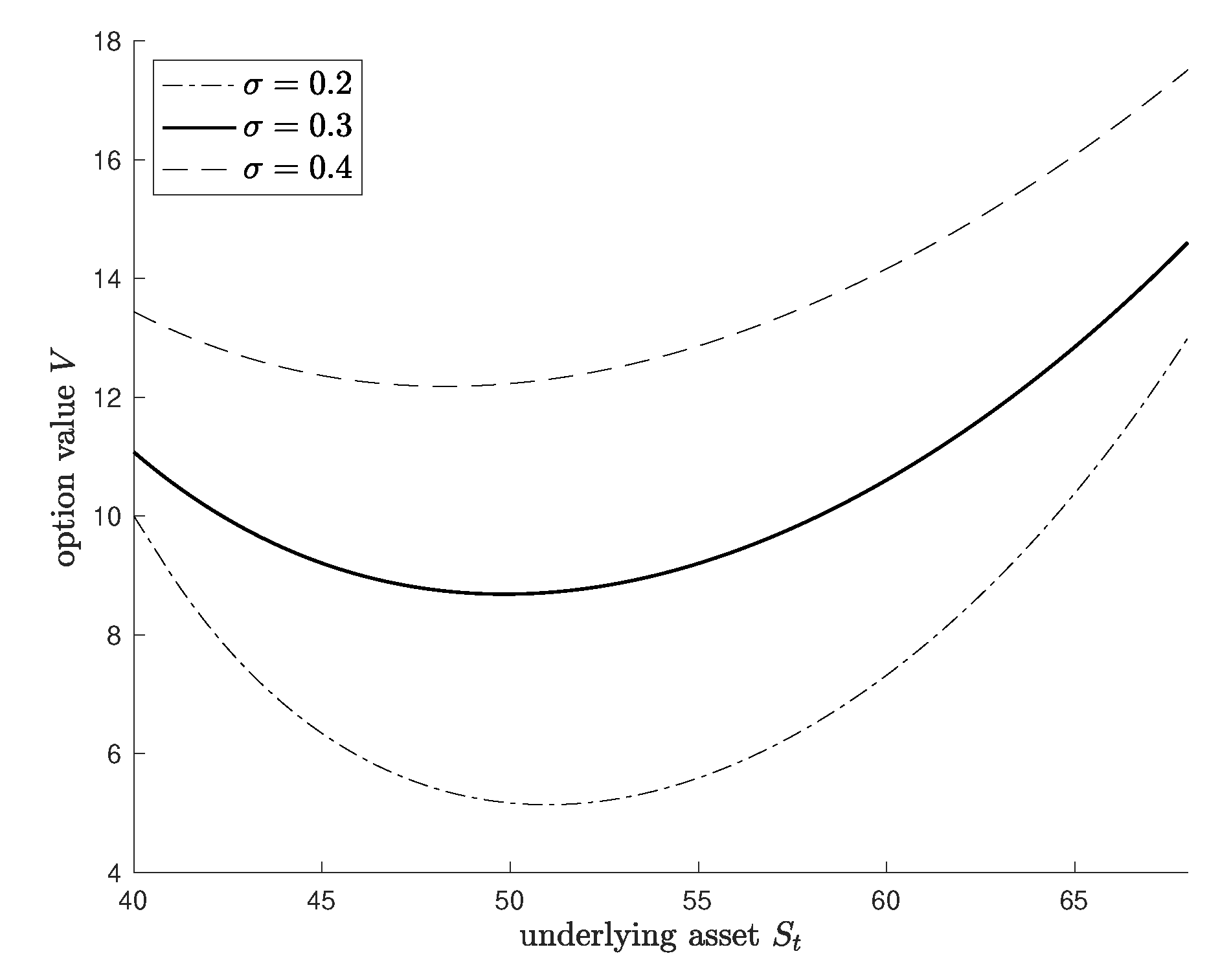
Figure 2 illustrates some curves of the optimal exercise boundaries against time to maturity $\tau$ and shows the effects of the mean-reversion speed $\kappa$ for American strangle option. In Figure 2, we observe that the waiting region becomes narrower as $\kappa$ increases. In Figure 3, we show option values with different $\kappa$ as the underlying asset changes. A higher value of $\kappa$ corresponds to a lower value of American strangle option. That is, the effect of the mean-reversion environment on the option can be seen in Figure 2 and Figure 3. In addition, Figure 4 and Figure 5 show how the optimal exercise boundaries and option values move as volatility $\sigma$ changes. When the value of $\sigma$ is low, the waiting region becomes narrower and the option value is low, as expected.

Figure 2. Two free boundaries ${\mathcal{Z}}_{\mathrm{up}}(t)$ and ${\mathcal{Z}}_{\mathrm{low}}(t)$ with respect to $\kappa$.

Figure 3. The option values at time $t=0$ with respect to $\kappa$.

Figure 4. Two free boundaries ${\mathcal{Z}}_{\mathrm{up}}(t)$ and ${\mathcal{Z}}_{\mathrm{low}}(t)$ with respect to $\sigma$.

Figure 5. The option values at time $t=0$ with respect to $\sigma$.

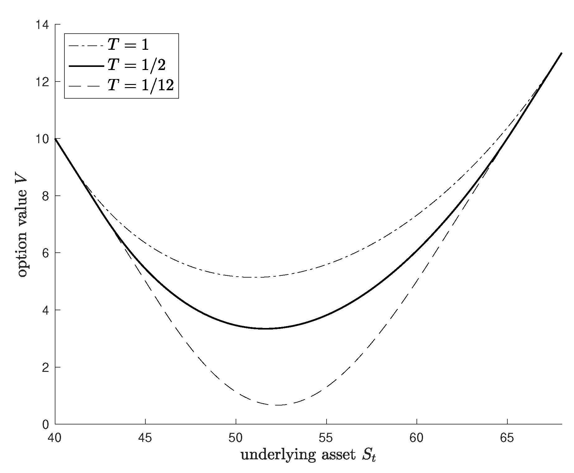
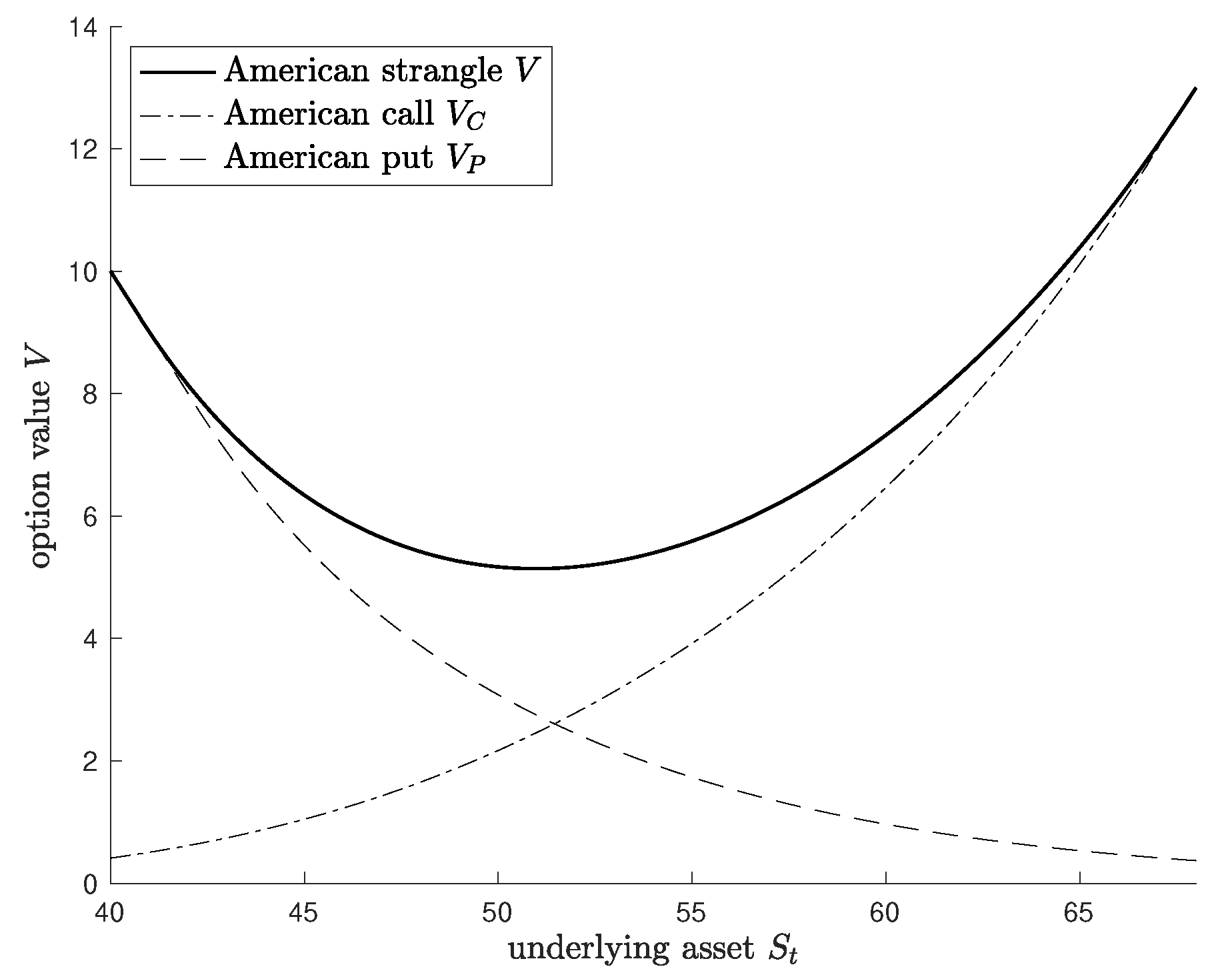
In Figure 6, we show option values with different maturity T. Although the option values are similar when the option is “In The Money” or “Out of The Money”, there seems to be a significant difference when the option is near to “At The Money”. In other words, when $S_t⟶0$ or $S_t⟶\infty$, the maturity has no effect on option values. Figure 7 and Figure 8 show the comparison of the optimal exercise boundaries and option values for three types of American options (call, put, strangle), respectively. Figure 7 shows that there is no difference in value at short $\tau$ and a slight difference at long $\tau$. The value function (V) of the American strangle option for the underlying asset is convex, as expected, unlike the American call ($V_C$) and American put ($V_P$) options, as illustrated in Figure 8. Moreover, it can be observed that V and $V_P$ get closer as $S_t$ decreases and V and $V_C$ get closer as $S_t$ increases.

Figure 6. The option values V at time $t=0$ with respect to the maturity T.

Figure 7. The comparison of the two free boundaries with those of the American call and put options, respectively.

Figure 8. The comparison of the option values with those of the American call and put options, respectively.

5. Concluding Remarks

We investigated a pricing model for the American strangle option in the mean-reversion environment in this paper. To describe the mean-reversion environment, we assumed that the underlying asset was driven by a mean-reverting process. Because an American strangle option incorporates simultaneously buying or selling call and put options on the same underlying asset, it has two free boundaries. Based on the PDE approach, we provided an analytical pricing formula for the American strangle option in the proposed model. Using Mellin transform techniques, we derived the integral equation representation for two optimal exercise boundaries arising from the nonhomogeneous PDE for the American strangle option price with finite maturity. The Mellin transforms have the advantage of converting the given PDE into a relatively simple ODE. After solving the ODE with some techniques, we used inverse Mellin transforms to invert the ODE solutions to obtain the integral equations for the American strangle option. Finally, the pricing formula was explicitly presented as the sum of the European call option, the European put option, and the early exercise premium, and it was quickly solved using the RIM. Based on our approach, we also investigated American call and put options in the mean-reversion environment.

Through numerical experiments, we verified the accuracy of our formula and investigated the impact of mean-reversion on the American strangle option. Numerical simulations using the MC simulation method showed that our formula was accurate and efficient. Furthermore, we showed how to move American strangle option prices with respect to several significant parameters using graphs, and we compared two free boundaries and values for three types of options (American call, American put, American strangle).

Although we provide meaningful results for the valuation of the American strangle option in a mean-reversion environment, this study has some limitations. First, we assumed that the underlying asset’s volatility was constant. The stochastic volatility model can be considered our model’s generalization. Second, the empirical analysis was not provided. In the future, these will be considered extended works.

References

- Black, F.; Scholes, M. The pricing of options and corporate liabilities. J. Political Econ. 1973, 81, 637–654. [Google Scholar] [CrossRef]
- Cox, J.C.; Ross, S.A.; Rubinstein, M. Option pricing: A simplified approach. J. Financ. Econ. 1979, 7, 229–263. [Google Scholar] [CrossRef]
- Boyle, P.P. A lattice framework for option pricing with two state variables. J. Financ. Quant. Anal. 1988, 23, 1–12. [Google Scholar] [CrossRef]
- Tian, Y. A modified lattice approach to option pricing. J. Futur. Mark. (1986–1998) 1993, 13, 563. [Google Scholar] [CrossRef]
- Brennan, M.J.; Schwartz, E.S. Finite difference methods and jump processes arising in the pricing of contingent claims: A synthesis. J. Financ. Quant. Anal. 1978, 13, 461–474. [Google Scholar] [CrossRef]
- Courtadon, G. A more accurate finite difference approximation for the valuation of options. J. Financ. Quant. Anal. 1982, 17, 697–703. [Google Scholar] [CrossRef]
- Johnson, H.E. An analytic approximation for the American put price. J. Financ. Quant. Anal. 1983, 18, 141–148. [Google Scholar] [CrossRef]
- Geske, R.; Johnson, H.E. The American put option valued analytically. J. Financ. 1984, 39, 1511–1524. [Google Scholar] [CrossRef]
- Kim, I.J. The analytic valuation of American options. Rev. Financ. Stud. 1990, 3, 547–572. [Google Scholar] [CrossRef]
- Jacka, S.D. Optimal stopping and the American put. Math. Financ. 1991, 1, 1–14. [Google Scholar] [CrossRef]
- Longstaff, F.; Schwartz, E. Valuing American Options by Simulation: A Simple Least-Squares Approach. Rev. Financ. Stud. 2001, 14, 113–147. [Google Scholar] [CrossRef]
- Rogers, L.C. Monte Carlo valuation of American options. Math. Financ. 2002, 12, 271–286. [Google Scholar] [CrossRef]
- Park, K.; Jeon, J. A simple and fast method for valuing American knock-out options with rebates. Chaos Solitons Fractals 2017, 103, 364–370. [Google Scholar] [CrossRef]
- Kang, M.; Jeon, J.; Han, H.; Lee, S. Analytic solution for American strangle options using Laplace–Carson transforms. Commun. Nonlinear Sci. Numer. Simul. 2017, 47, 292–307. [Google Scholar] [CrossRef]
- Zaevski, T.S. A new form of the early exercise premium for American type derivatives. Chaos Solitons Fractals 2019, 123, 338–340. [Google Scholar] [CrossRef]
- Lee, J.K. A simple numerical method for pricing American power put options. Chaos Solitons Fractals 2020, 139, 110254. [Google Scholar] [CrossRef]
- Deng, G. Pricing perpetual American floating strike lookback option under multiscale stochastic volatility model. Chaos Solitons Fractals 2020, 141, 110411. [Google Scholar] [CrossRef]
- Qiu, S. American strangle options. Appl. Math. Financ. 2020, 27, 228–263. [Google Scholar] [CrossRef]
- Zaevski, T.S. A new approach for pricing discounted American options. Commun. Nonlinear Sci. Numer. Simul. 2021, 97, 105752. [Google Scholar] [CrossRef]
- Jeon, J.; Kim, G. An integral equation representation for American better-of option on two underlying assets. Adv. Contin. Discret. Model. 2022, 2022, 39. [Google Scholar] [CrossRef]
- Zaevski, T.S. Pricing discounted American capped options. Chaos Solitons Fractals 2022, 156, 111833. [Google Scholar] [CrossRef]
- Sorensen, C. An equilibrium approach to pricing foreign currency options. Eur. Financ. Manag. 1997, 3, 63–84. [Google Scholar] [CrossRef]
- Hui, C.; Lo, C. Currency barrier option pricing with mean reversion. J. Futur. Mark. 2006, 26, 939–958. [Google Scholar] [CrossRef]
- Wong, H.; Lau, K. Path-dependent currency options with mean reversion. J. Futur. Mark. 2008, 29, 275–293. [Google Scholar] [CrossRef]
- Panini, R. Option Pricing with Mellin Transforms; State University of New York at Stony Brook: Stony Brook, NY, USA, 2004. [Google Scholar]
- Frontczak, R.; Schöbel, R. On modified Mellin transforms, Gauss–Laguerre quadrature, and the valuation of American call options. J. Comput. Appl. Math. 2010, 234, 1559–1571. [Google Scholar] [CrossRef][Green Version]
- Rodrigo, M.R. Approximate ordinary differential equations for the optimal exercise boundaries of American put and call options. Eur. J. Appl. Math. 2014, 25, 27–43. [Google Scholar] [CrossRef]
- Jeon, J.; Han, H.; Kang, M. Valuing American floating strike lookback option and Neumann problem for inhomogeneous Black–Scholes equation. J. Comput. Appl. Math. 2017, 313, 218–234. [Google Scholar] [CrossRef]
- Huang, J.Y.; Subrahmanyam, M.; Yu, G. Pricing and hedging American options: A recursive integration method. Rev. Financ. Stud. 1996, 9, 277–300. [Google Scholar] [CrossRef]
- Jeon, J.; Kim, G. Pricing European continuous-installment strangle options. N. Am. J. Econ. Financ. 2019, 50, 101049. [Google Scholar] [CrossRef]
- Jeon, J.; Kwak, M. Pricing Variable Annuity with Surrender Guarantee. J. Comput. Appl. Math. 2021, 393, 113508. [Google Scholar] [CrossRef]
- Erdlyi, A.; Magnus, W.; OberhettingerF, F.; Tricomi, F. Tables of Integral Transforms; McGraw-Hill: New York, NY, USA, 1954. [Google Scholar]
- Sneddon, I. The Use of Integral Transforms; McGraw-Hill: New York, NY, USA, 1972. [Google Scholar]
- Bertrand, J.; Bertrand, P.; Ovarlez, J. The Mellin Transform; CRC Press: Boca Raton, FL, USA, 2000. [Google Scholar]
Publisher’s Note: MDPI stays neutral with regard to jurisdictional claims in published maps and institutional affiliations. |
© 2022 by the authors. Licensee MDPI, Basel, Switzerland. This article is an open access article distributed under the terms and conditions of the Creative Commons Attribution (CC BY) license (https://creativecommons.org/licenses/by/4.0/).