Reduced Basis Approximation for a Spatial Lotka-Volterra Model

Abstract

We construct a reduced basis approximation for the solution to a system of nonlinear partial differential equations describing the temporal evolution of two populations following the Lotka-Volterra law. The first population’s carrying capacity contains a free parameter varying in a compact set. The reduced basis is constructed by two approaches: a proper orthogonal decomposition of a collection of solution snapshots and a greedy algorithm using an a posteriori error estimator.

1. Introduction

The reduced basis method finds applications in the construction of approximate solutions to parametrised partial differential equations using carefully chosen low-dimensional projection of the solution manifold associated with the compact set where the parameter varies. Whenever the problem needs to be solved in a multi-query context (for instance, for the needs of an optimisation problem), or for multiple parameter values, a direct approach based on repeated solutions could incur a very high computational cost. The goal of the method is to approximate the solution by computing its coefficients in an orthonormal basis, which is low-dimensional compared to the high-dimensional Galerkin finite element basis used in a standard discretisation scheme. Thus, the solutions for different parameter values as well as the approximation error can be approximated from a problem of much lower dimension.

Recent applications of the method include problems from physics and engineering such as fluid dynamics [1,2], viscous Burgers equation [3], the Navier–Stokes equations [4,5], and linear parabolic problems [6,7,8]. Achieving such a reduced basis approximation with reasonable accuracy and reduced computational effort depends on the solution manifold being of low dimension as well as the problem’s regularity and affine dependence on the free parameter.

This method has not yet been applied to evolution problems stemming from biological applications, which often contain nonlinear terms, coupling of multiple variables as well as require appropriate stable numerical schemes for time integration. Partial differential equations of reaction-diffusion type are employed, for example, in modelling the immune response to infections [9,10] and tumour growth and onco-immune interactions [11,12].

We study the performance of the reduced-basis method for a problem motivated by a biomedical application (tumour growth under chemotherapy). In particular, we take as example the parametrised Lotka-Volterra reaction-diffusion model over a bounded convex domain $\Omega \subset {\mathbb{R}}^2$ with Lipschitz boundary, where the reaction part contains a free parameter. This model describes the evolution of the unknown $u=(u_1,u_2)$ where $u_i(x,y,t)\ge 0,i=1,2$ represent the densities of two competing populations at $(x,y)\in \Omega$ at time $t\in [0,T_{\mathrm{end}}]$. The model reads

$${\partial }_t{u}_i=d_i\Delta u_i+f_i(u;\mu ),i=1,2$$

(1)

where the diffusion rate for i-th population is $d_i>0$, and the growth rate of the populations is given by a nonlinear vector function f:

$$f(u;\mu )={(u_1(a_1-\mu -u_1-c_1{u}_2),u_2(a_2-u_2-c_2{u}_1))}^T.$$

(2)

Here, $a_i,c_i>0$ denote the carrying capacity and strength of competition, and the free parameter is $\mu \in \mathcal{M}\subset {\mathbb{R}}_{+}$, with $\mathcal{M}$ being a compact set. A growth rate like (2) (without diffusion in space) has been used in [13] to model changes in the tumour composition. In particular, (1) shall model the interactions between populations of chemotherapy-sensitive cancer cells $u_1$ and chemotherapy-resistant cancer cells $u_2$. The death (or loss) of sensitive cellls $u_1$ due to chemotherapy with dose $\mu$ is encoded in the term $-\mu u_1$. The system (1) is complemented by initial conditions $u(·,0)\ne 0$ and Dirichlet boundary condition, $u(·,t)=0$ on $\partial \Omega$.

2. Problem Statement

In this work, we construct a reduced basis approximation of the solutions to (1) based on a Galerkin (finite element) approximation. This reduced basis is low-dimensional compared to the dimension of the finite element approximation space, and is used to compute efficiently approximate solutions to (1) for different values of $\mu$. For the construction of the reduced basis, we use two approaches: a proper orthogonal decomposition (POD) and a POD-greedy algorithm based on an a posteriori error estimator for the approximation error, and compare their performance.

We denote by $L^1(\Omega ),L^2(\Omega ),L^{\infty }(\Omega )$ the spaces of measurable functions on $\Omega$ that are respectively Lebesgue-integrable, square-integrable or have a bounded essential supremum, and $H_0^1(\Omega )$ the Sobolev space of functions $w\in L^2(\Omega )$ vanishing on $\partial \Omega$ with ${\int }_{\Omega }\nabla w·\nabla w<\infty$. Here, $\nabla w$ denotes the gradient $({\partial }_{x}w,{\partial }_{y}w)$. Tensor spaces such as $L^p\times L^p$ inherit the respective norms from $L^p$, etc.

Given an initial value $u(·,0)\in H_0^1\times H_0^1$, (1) has unique solutions in time and under certain conditions on the diffusion rates $d_i$ and the parameters (e.g., $c_i<1$) admit nontrivial, nonnegative stationary in time solutions [14]. We assume such parameter values in this work.

A Galerkin finite element method applied to the Laplace operator in (1) makes the resulting semi-discrete system stiff. Since the problem is a pure reaction-diffusion problem, an implicit Euler scheme is a reasonable choice for time integration. The approximation of the time derivative ${\partial }_{t}u$ is based on the solutions at consecutive time layers $u^k=u(·,k\tau )$ for appropriately chosen time step $\tau >0$ to guarantee stability of the scheme. We consider henceforth the scheme:

$$\begin{array}{cc}\hfill \frac{1}{\tau }{⟨u^k,\varphi ⟩}_2& +\alpha (u^k,\varphi )-{⟨f(u^k;\mu ),\varphi ⟩}_2=\frac{1}{\tau }{⟨u^{k-1},\varphi ⟩}_2\hfill \end{array}$$

(3)

In (3), we denote the inner product

$${⟨u,v⟩}_2\stackrel{\mathrm{def}}{=}{\int }_{\Omega }(u_1{v}_1+u_2{v}_2)dx,u,v\in L^2\times L^2,$$

and the bilinear form

$$\alpha (u,v)\stackrel{\mathrm{def}}{=}{\int }_{\Omega }{d}_1\nabla u_1·\nabla v_1+d_2\nabla u_2·\nabla v_{2}dx,u,v\in H_0^1\times H_0^1.$$

(4)

Equation (4) defines the energy norm ${\parallel ·\parallel }_{\alpha }$ via ${\parallel w\parallel }_{\alpha }^2\stackrel{\mathrm{def}}{=}\alpha (w,w)$ for $w\in H_0^1\times H_0^1$. Friedrich’s inequality [15] implies that the energy norm ${\parallel ·\parallel }_{\alpha }$ and the $H_0^1$-induced norm are equivalent on $H_0^1\times H_0^1$.

3. Reduced Basis

Let ${\mathcal{T}}_h$ be a triangulation of $\Omega$. We use a Galerkin approximation with a finite element space ${\mathbb{V}}_h\stackrel{\mathrm{def}}{=}{\mathbb{W}}_h\times {\mathbb{W}}_h$, where ${\mathbb{W}}_h\subset H_0^1(\Omega )$ is spanned by finite element functions whose restriction on each element of ${\mathcal{T}}_h$ is piecewise polynomial of a fixed degree. In other words, the pair $({\mathcal{T}}_h,{\mathbb{W}}_h)$ is assumed to satisfy classical assumptions on regularity, affine equivalence and compact support of the finite element functions ([15], p. 132). At this stage, we assume that ${\mathcal{T}}_h$ and ${\mathbb{W}}_h$ approximate the solution to (3) with sufficient accuracy and further details on ${\mathbb{W}}_h$ shall be provided later.

The space ${\mathbb{V}}_h$ shall be referred to as truth space or high fidelity approximation space [16,17]. For a given $\mu \in \mathcal{M}$, let the solution snapshot of (3) in the truth space be given by the sequence of functions $U_h\left(\mu \right)=\{u_h^k\left(\mu \right)\in {\mathbb{V}}_h:k=0,1,\dots k_{max}\}$ that contains the values of $u_h^k\left(\mu \right)$ on time layers $t=k\tau ,k=0,1,\dots k_{max}$ with $k_{max}\tau =T_{\mathrm{end}}$.

A reduced basis serving to approximate the solutions of (3) in the truth space for all $\mu \in \mathcal{M}$ is given by functions ${\left\{{\xi }_i\right\}}_{i=1}^N\in {\mathbb{V}}_h$ defining an orthonormal basis for a subspace of dimension $N\ll \dim {\mathbb{V}}_h$. As long as a reduced basis approximation is possible, the basis elements are constructed so that the approximation error (in some norm to be defined later) between $U_h\left(\mu \right)$ and the reduced basis solution $U_{\mathrm{rb}}\left(\mu \right)\in {\mathbb{V}}_{\mathrm{rb}}^N\stackrel{\mathrm{def}}{=}\mathrm{span}{\left\{{\xi }_i\right\}}_{i=1}^N$ stays within a prescribed tolerance $\epsilon$. Furthermore, the computational cost of the solution $U_{\mathrm{rb}}\left(\mu \right)$ for every different parameter value $\mu$ shall remain independent of $\dim {\mathbb{V}}_h$.

3.1. Numerical Scheme for Integration in Time

Problem (3) is a nonlinear equation for $u_h^k\left(\mu \right)$, which can be solved using Newton’s method at each time layer k. Denote the linear functional

$$\mathbf{G}(\psi ,\varphi ;u_h^{k-1}\left(\mu \right))\stackrel{\mathrm{def}}{=}\frac{1}{\tau }{⟨\psi ,\varphi ⟩}_2+\alpha (\psi ,\varphi )-{⟨f(\psi ;\mu ),\varphi ⟩}_2-\frac{1}{\tau }{⟨u_h^{k-1}\left(\mu \right),\varphi ⟩}_2,\psi ,\varphi \in {\mathbb{V}}_h$$

and the bilinear form

$$\mathbf{DG}(\psi ,\varphi ;\mu ,{\psi }^s)\stackrel{\mathrm{def}}{=}\frac{1}{\tau }{⟨\psi ,\varphi ⟩}_2+\alpha (\psi ,\varphi )-{⟨\mathbf{J}({\psi }^s;\mu )\psi ,\varphi ⟩}_2,\psi ,\varphi \in {\mathbb{V}}_h,$$

(5)

where $\mathbf{J}$ is the Jacobian of f at u:

$$\mathbf{J}(u;\mu )=\left(\begin{array}{cc}{a}_1-\mu -2u_1-c_1{u}_2& -c_1{u}_1\\ -c_2{u}_2& a_2-c_2{u}_1-2u_2\end{array}\right).$$

Note that $\mathbf{J}$ is bounded for $u\in {\mathbb{V}}_h$. We solve for $u_h^k=\psi$ from $\mathbf{G}(\psi ,\varphi ;u_h^{k-1}\left(\mu \right))=0$. $\psi$ can be approximated by successive Newton iterations (Algorithm 1):

Algorithm 1 Newton iteration.

Require:${\psi }^0,u_h^{k-1}\left(\mu \right),{\epsilon }_{Newton}$   while $\parallel \mathbf{G}({\psi }^s,\varphi ;u_h^{k-1}\left(\mu \right))\parallel >{\epsilon }_{Newton}$ do    solve $$\hspace{1em}\hspace{1em}\hspace{1em}\hspace{1em}\hspace{1em}\hspace{1em}\hspace{1em}\hspace{1em}\hspace{1em}\hspace{1em}\mathbf{DG}({\delta }^s,\varphi ;\mu ,{\psi }^s)=-\mathbf{G}({\psi }^s,\varphi ;u_h^{k-1}\left(\mu \right))$$ (6)    set ${\psi }^{s+1}={\psi }^s+{\delta }^s,s=s+1$ end while Return: $\psi ={\psi }^s$

Lemma 1 together with the Lax–Milgram lemma [18] ensure that (6) has a unique solution in ${\mathbb{V}}_h$.

Lemma 1.

For all $\mu \in \mathcal{M}$, the form $\mathbf{DG}(·,·;\mu ,y)$ in (5) is continuous on ${\mathbb{V}}_h$ and coercive on ${\mathbb{V}}_h$ for $\tau <\max \frac{1}{a_i}$ .

Proof. 

We need to estimate the coercivity and continuity factors for $\mathbf{DG}(·,·;\mu ,y)$ (those depend on $\mu$).

For the continuity factor, we use Hölder’s inequality and Poincaré’s inequality for $v,w\in {\mathbb{V}}_h$. Below, $C_{\Omega }$ denotes the constant from Poincaré’s inequality [15] for ${\mathbb{W}}_h$.

$$\left|\mathbf{DG}(v,w;\mu ,u)\right|\le \left|\alpha (v,w)\right|+|{⟨(\frac{1}{\tau }-\mathbf{J}(u;\mu ))v,w⟩}_2{|\le \gamma (u,\mu )\parallel v\parallel }_{\alpha }{\parallel w\parallel }_{\alpha }$$

with

$$\gamma (u,\mu )=\sqrt{2}+C_{\Omega }\left[\frac{1}{\tau }+\underset{\Omega }{\sup }\rho \left(\mathbf{J}(u;\mu )\right)\right],$$

where $\rho \left(\mathbf{J}\right(u;\mu \left)\right)$ denotes the spectral radius of $\mathbf{J}(u,\mu )$ .

For the coercivity, we obtain $\mathbf{DG}(v,v;\mu ,u)=\alpha (v,v)+{⟨(\frac{1}{\tau }-\mathbf{J}(u;\mu ))v,v⟩}_2$ and

$$\begin{array}{c}{⟨(\frac{1}{\tau }-\mathbf{J}(u;\mu ))v,v⟩}_2={\int }_{\Omega }\left(\begin{array}{c}(\frac{1}{\tau }-a_1+\mu )v_1\\ (\frac{1}{\tau }-a_2)v_2\end{array}\right)·\left(\begin{array}{c}{v}_1\\ v_2\end{array}\right)+\left(\begin{array}{c}(2u_1+c_1{u}_2)v_1+c_1{u}_1{v}_2\\ c_2{u}_2{v}_1+(c_2{u}_1+2u_2)v_2\end{array}\right)·\left(\begin{array}{c}{v}_1\\ v_2\end{array}\right)\hfill \\ ={\int }_{\Omega }\left[(\frac{1}{\tau }-a_1+\mu )v_1^2+(\frac{1}{\tau }-a_2)v_2^2\right]\\ \hfill +{\int }_{\Omega }(2u_1+c_1{u}_2)v_1^2+(c_1{u}_1+c_2{u}_2)v_1{v}_2+(c_2{u}_1+2u_2)v_2^2.\end{array}$$

By assumption $c_1,c_2<1$, the last form is positive semidefinite for $u_1,u_2\ge 0$ because

$$\begin{array}{c}{(c_1{u}_1+c_2{u}_2)}^2-4(2u_1+c_1{u}_2)(c_2{u}_1+2u_2)=\hfill \\ \hfill \hspace{1em}\hspace{1em}\hspace{1em}\hspace{1em}\hspace{1em}\hspace{1em}\hspace{1em}\hspace{1em}\hspace{1em}\hspace{1em}\hspace{1em}\hspace{1em}-2c_1{c}_2{u}_1{u}_2-16u_1{u}_2+(c_1^2-8c_1)u_1^2+(c_2^2-8c_2)u_2^2\le 0.\end{array}$$

Hence, ${⟨(\frac{1}{\tau }-\mathbf{J}(u;\mu ))v,v⟩}_2\ge \min \{\frac{1}{\tau }-a_1+\mu ,\frac{1}{\tau }-a_2\}{\parallel v\parallel }_2$, implying that, for the chosen $\tau$, $\mathbf{DG}(v,v;\mu ,u)\ge {\parallel v\parallel }_{\alpha }^2$. □

3.2. Offline and Online Phases

The chosen time integration scheme is used to construct the reduced basis elements ${\xi }_i$. during the offline stage. Snapshots $U_h\left({\mu }^{\ast }\right)$ for carefully sampled values ${\mu }^{\ast }\in \mathcal{M}$ are used to generate the reduced basis elements via a POD or a POD-greedy algorithm [6,7,16,17]. The training set $\Xi \subset \mathcal{M}$ for sampling must be chosen sufficiently rich to provide a good approximation property of the resulting reduced basis. During this stage, all parameter-independent objects (stiffness matrices and load vectors) required for the discrete solution in ${\mathbb{V}}_{\mathrm{rb}}^N$ are computed and stored.

Assume that the reduced basis space ${\mathbb{V}}_{\mathrm{rb}}^N\subset {\mathbb{V}}_h$ with $N\ll \dim {\mathbb{V}}_h$ has already been found. Let $u_{\mathrm{rb}}^k\left(\mu \right)$ be the approximation in ${\mathbb{V}}_{\mathrm{rb}}^N$ to the solution $u_h^k\left(\mu \right)$ in the truth space at time layer $t=k\tau$ for a given $\mu$. During the online stage, the computation of $U_{\mathrm{rb}}\left(\mu \right)$ for a new parameter value $\mu$ shall involve the assembly of stiffness matrices and load vectors for the low-dimensional problem from those obtained during the offline phase.

3.3. Solving the Problem in the Reduced Basis

The expansion coefficients ${\mathbf{u}}_k^{\mu }={\left\{{\mathbf{u}}_{k,i}^{\mu }\right\}}_{i=1}^N$ in the reduced basis will be computed by solving a problem in N dimensions. Let

$$u_{\mathrm{rb}}^k\left(\mu \right)=\sum _{i=1}^N{\mathbf{u}}_{k,i}^{\mu }{\xi }_i.$$

(7)

Using scheme (3), we solve for the reduced basis solution $u_{\mathrm{rb}}^k\left(\mu \right)$. We let $\varphi ={\xi }_j,1\le j\le N$ in (6) and obtain a linear system for ${\mathbf{u}}_k^{\mu }$. For the Newton iteration step, we set

$${\mathbf{x}}^s=\sum _{i=1}^N{\mathbf{x}}_i^s{\xi }_i,\delta =\sum _{i=1}^N{\delta }_i{\xi }_i$$

which transforms (6) into an N-dimensional system. Then, we follow an analogous Algorithm 2:

Algorithm 2 Newton iteration reduced basis.

Require:${\mathbf{x}}^0,{\mathbf{u}}_{k-1}^{\mu },{\epsilon }_{Newton}$   while  $\parallel \mathbf{G}({\sum }_{i=1}^N{\mathbf{y}}_i^s{\xi }_i,{\xi }_j,\mu ;{\mathbf{u}}_{k-1,i}^{\mu }){\parallel }_2>{\epsilon }_{Newton}$ do   solve $$\hspace{1em}\hspace{1em}\hspace{1em}\hspace{1em}\hspace{1em}\hspace{1em}\hspace{1em}\hspace{1em}\hspace{1em}\hspace{1em}\mathbf{DG}({\xi }_i,{\xi }_j,\mu ;{\mathbf{x}}^s)\delta =-\mathbf{G}(\sum _{i=1}^N{\mathbf{x}}_i^s{\xi }_i,{\xi }_j,\mu ;{\mathbf{u}}_{k-1,i}^{\mu })$$ (8)   set ${\mathbf{x}}^{s+1}={\mathbf{x}}^s+\delta ,s=s+1$   end while   Return: ${\mathbf{u}}_k^{\mu }={\mathbf{x}}^s$

Note that (8) admits a unique solution as a consequence of the well-posedness of the truth scheme (6), and the inclusion ${\mathbb{V}}_{\mathrm{rb}}^N\subset {\mathbb{V}}_h$ ([17], Lemma 3.1).

We now present the matrix formulation for the offline stage of (8), and rewrite the matrix $\mathbf{DG}$ and the functional $\mathbf{G}$ in terms of the reduced basis elements ${\xi }_i$: Denote the matrices

$${\mathcal{A}}_N=\left(\begin{array}{cc}{a}_1{\mathbb{I}}_N& 0\\ 0& a_2{\mathbb{I}}_N\end{array}\right),{\mathcal{C}}_N=\left(\begin{array}{cc}0& c_1{\mathbb{I}}_N\\ c_2{\mathbb{I}}_N& 0\end{array}\right),{\mathcal{I}}_N=\left(\begin{array}{cc}{\mathbb{I}}_N& 0\\ 0& 0\end{array}\right)$$

where ${\mathbb{I}}_m,m\in \mathbb{N}$ is the $m\times m$ identity matrix. In fact, we have (in matrix-vector notation): $f(w,\mu )=({\mathcal{A}}_N-{\mathcal{I}}_N)w-w^2-w^T{\mathcal{C}}_{N}w$.

Define the matrices $\mathbb{M},\mathbb{A},{\mathbb{B}}_1,{\mathbb{B}}_2$ via

$${\left(\mathbb{M}\right)}_{ij}\stackrel{\mathrm{def}}{=}{⟨{\xi }_i,{\xi }_j⟩}_2,{\left(\mathbb{A}\right)}_{ij}\stackrel{\mathrm{def}}{=}\alpha ({\xi }_i,{\xi }_j),{\left({\mathbb{B}}_1\right)}_{ij}\stackrel{\mathrm{def}}{=}{⟨{\mathcal{A}}_N{\xi }_i,{\xi }_j⟩}_2,{\left({\mathbb{B}}_2\right)}_{ij}\stackrel{\mathrm{def}}{=}{⟨{\mathcal{I}}_N{\xi }_i,{\xi }_j⟩}_2,i,j=1,\dots ,N.$$

Denote the following trilinear forms:

$${\beta }_0({\xi }_i,{\xi }_j,{\xi }_l)\stackrel{\mathrm{def}}{=}{\int }_{\Omega }{\xi }_i{\xi }_j{\xi }_l,{\beta }_1({\xi }_i,{\xi }_j,{\xi }_l)\stackrel{\mathrm{def}}{=}{\int }_{\Omega }\left({\mathcal{C}}_N{\xi }_i\right){\xi }_j{\xi }_l,{\beta }_2({\xi }_i,{\xi }_j,{\xi }_l)\stackrel{\mathrm{def}}{=}{\int }_{\Omega }{\xi }_i\left({\mathcal{C}}_N{\xi }_j\right){\xi }_l,$$

which are used to define the matrix

$$\mathbb{L}\left(\mathbf{y}\right):{\left(\mathbb{L}\right)}_{ij}\left(\mathbf{y}\right)\stackrel{\mathrm{def}}{=}-\sum _{l=1}^N{\mathbf{y}}_l\sum _{m=0}^2{\beta }_m({\xi }_l,{\xi }_i,{\xi }_j),\mathbf{y}\in {\mathbb{R}}^N$$

and the arrays of matrices ${\mathbb{P}}^j,{\mathbb{Q}}^j,j=1,\dots ,N$ defined by

$${\left({\mathbb{P}}^j\right)}_{i_1{i}_2}\stackrel{\mathrm{def}}{=}{\beta }_0({\xi }_{i_1},{\xi }_{i_2},{\xi }_j),{\left({\mathbb{Q}}^j\right)}_{i_1{i}_2}\stackrel{\mathrm{def}}{=}{\beta }_2({\xi }_{i_1},{\xi }_{i_2},{\xi }_j)$$

with $i_1,i_2=1,\dots ,N$.

To evaluate the nonlinear terms inside (8) in the reduced basis setting, we have to compute the following vectors in ${\mathbb{R}}^N$: $\mathbb{P}\left(\mathbf{y}\right)\stackrel{\mathrm{def}}{=}{\left\{{\mathbf{y}}^T{\mathbb{P}}^j\mathbf{y}\right\}}_{j=1}^N,\mathbb{Q}\left(\mathbf{y}\right)\stackrel{\mathrm{def}}{=}{\left\{{\mathbf{y}}^T{\mathbb{Q}}^j\mathbf{y}\right\}}_{j=1}^N$ for appropriate $\mathbf{y}\in {\mathbb{R}}^N$.

In this matrix notation, we rewrite the linear problem (8) as:

$$\begin{array}{cc}\hfill \mathbb{DG}(\mu ,{\mathbf{x}}^s)\delta & =-\mathbb{G}(\mu ,{\mathbf{x}}^s,{\mathbf{u}}_{k-1}^{\mu })\mathrm{where}\hfill \\ \hfill \mathbb{DG}(\mu ,{\mathbf{x}}^s)& =\frac{1}{\tau }\mathbb{M}+\mathbb{A}-{\mathbb{B}}_1+\mu {\mathbb{B}}_2+\mathbb{L}\left({\mathbf{x}}^s\right)\hfill \\ \hfill \mathbb{G}(\mu ,{\mathbf{x}}^s,{\mathbf{u}}_{k-1}^{\mu })& =\frac{1}{\tau }\mathbb{M}({\mathbf{x}}^s-{\mathbf{u}}_{k-1}^{\mu })+\mathbb{A}{\mathbf{y}}^s-{\mathbb{B}}_1{\mathbf{x}}^s+\mu {\mathbb{B}}_2{\mathbf{x}}^s+\mathbb{P}\left({\mathbf{x}}^s\right)+\mathbb{Q}\left({\mathbf{x}}^s\right)\hfill \end{array}$$

(9)

where the objects $\mathbb{M},\mathbb{A},{\mathbb{B}}_1,{\mathbb{B}}_2,{\mathbb{P}}^i,{\mathbb{Q}}^i,i=1,\dots ,N$ are matrices or arrays of matrices that are independent of $\mu$. Finally, the solution resulting from the reduced basis approximation is recovered from ${\mathbf{u}}_k^{\mu }$ via (7).

3.4. Reduced Basis Construction via the POD-Greedy Algorithm

The greedy algorithm is used for construction of reduced basis approximations in the context of elliptic problems (see [16,17] for references). It enriches at every iteration the constructed reduced basis by adding an additional snapshot associated with the parameter value ${\mu }^{\ast }$ that maximises the approximation error (in some norm) between the snapshot $U_h\left(\mu \right)$ and its approximation $U_{\mathrm{rb}}\left(\mu \right)$ spanned by the reduced basis constructed thus far, in other words ${\mu }^{\ast }=\arg {\max }_{\mu \in \mathcal{M}}\parallel U_h\left(\mu \right)-U_{\mathrm{rb}}\left(\mu \right)\parallel$. An estimate of this error should be easily computable for various values of $\mu$. The performance of the greedy algorithm relies upon a sufficiently dense training subset $\mathsf{\Xi }=\{{\mu }_j,j=1,\dots m\}\subset \mathcal{M}$, which is used to find a good value for ${\mu }^{\ast }$.

In our context, the greedy algorithm is complemented by a proper orthogonal decomposition step (Algorithm 3). The motivation for this lies in (3) whose solutions converge to a stationary in time solution. The POD step minimises redundancy of storage of basis elements and prevents possible stalling of the algorithm.

Furthermore, the approximation error $\parallel U_h\left(\mu \right)-U_n\left(\mu \right)\parallel$ should be estimated by an a posteriori error estimator ${\Delta }_{\mathrm{rb}}\left(\mu \right),\forall \mu \in \mathcal{M}$, which is computationally inexpensive in order to serve as a stopping criterion in the POD-greedy algorithm. When the prescribed accuracy ${\epsilon }_{\mathrm{tol}}$ is reached, the algorithm returns the N-dimensional reduced basis ${\left\{{\xi }_i\right\}}_{i=1}^N$.

Algorithm 3 POD-greedy algorithm.

Require:${\epsilon }_{\mathrm{tol}},\Xi ,n_1,n_2\in \mathbb{N},n_2<n_1,{\mu }_1$ Ensure:$N=0,\ell =1,{\Delta }_{\mathrm{rb}}\left({\mu }_1\right)=2{\epsilon }_{\mathrm{tol}},\mathcal{Z}=⌀$   while  ${\Delta }_{\mathrm{rb}}\left({\mu }_{\ell }\right)>{\epsilon }_{\mathrm{tol}}$ do   compute snapshot $U_h\left({\mu }_{\ell }\right)$   compress $U_h\left({\mu }_{\ell }\right)$ using POD, retain $n_1$ principal nodes ${\left\{{\zeta }_j\right\}}_{j=1}^{n_1}$   set $\mathcal{Z}=\mathcal{Z}\cup {\left\{{\zeta }_j\right\}}_{j=1}^{n_1}$   if $\ell =1$ then     $N=n_1$   else     $N=N+n_2$     compress $\mathcal{Z}$ using POD, retain N principal nodes ${\left\{{\xi }_j\right\}}_{j=1}^N$     $\mathcal{Z}={\left\{{\xi }_j\right\}}_{j=1}^N$   end if   compute the error estimator ${\Delta }_{\mathrm{rb}}\left(\mu \right),\forall \mu \in \Xi$ using $\mathcal{Z}$ as basis   set ${\mu }_{\ell +1}=\arg {\max }_{\mu \in \Xi }{\Delta }_{\mathrm{rb}}\left(\mu \right),\Xi =\Xi \setminus {\mu }_{\ell +1},\ell =\ell +1$ end while Return: $\mathcal{Z},N$

3.5. A Posteriori Error Analysis

In line with the time integration scheme, we derive an a posteriori estimate for the approximation error between the solution in the truth space $u_h^k$ and in the reduced basis $u_{\mathrm{rb}}^k$ at the k-th time layer, $e_k\left(\mu \right)\stackrel{\mathrm{def}}{=}{u}_h^k\left(\mu \right)-u_{\mathrm{rb}}^k\left(\mu \right)\in {\mathbb{V}}_h$. Note that $f(·;\mu )$ is Lipschitz continuous on $[0,a_1]\times [0,a_2]$, so

$$|f(z;\mu )-f(z^{\prime };\mu )|\le {\ell }_f|z-z^{\prime }|.$$

(10)

Let the residual associated with $u_{\mathrm{rb}}^k$ be

$$r^k(\varphi ;\mu )={⟨f(u_{\mathrm{rb}}^k;\mu ),\varphi ⟩}_2-\frac{1}{\tau }{⟨u_{\mathrm{rb}}^k-u_{\mathrm{rb}}^{k-1},\varphi ⟩}_2-\alpha (u_{\mathrm{rb}}^k,\varphi ),\forall \varphi \in {\mathbb{V}}_h.$$

(11)

$r^k$ is a linear functional on ${\mathbb{V}}_h$, whose norm in the dual space ${\mathbb{V}}_h^{\prime }$ is

$$\parallel r^k{(·;\mu )\parallel }_{{\alpha }^{\prime }}\stackrel{\mathrm{def}}{=}\underset{\varphi \in {\mathbb{V}}_h}{\sup }\frac{|r^k(\varphi ;\mu )|}{{\parallel \varphi \parallel }_{\alpha }}.$$

(12)

the Riesz representation theorem, implies that there exists a unique ${\tilde{r}}^k\in {\mathbb{V}}_h$ such that

$$\alpha ({\tilde{r}}^k\left(\mu \right),\varphi )=r^k(\varphi ;\mu ),\forall \varphi \in {\mathbb{V}}_h,$$

and $\parallel r^k{(·;\mu )\parallel }_{{\alpha }^{\prime }}={\parallel {\tilde{r}}^k\left(\mu \right)\parallel }_{\alpha }$.

Because $r^k$ has an affine dependence on $\mu$, its norm can be efficiently computed. We have the following evolution equation for the error $e_k$ based on (3):

$$\frac{1}{\tau }{⟨e_k-e_{k-1},\varphi ⟩}_2+\alpha (e_k,\varphi )={⟨f(u_h^k;\mu )-f(u_{\mathrm{rb}}^k;\mu ),\varphi ⟩}_2+r^k(\varphi ;\mu ),k\ge 1,\forall \varphi \in {\mathbb{V}}_h.$$

(13)

The following result gives an estimate for the approximation error $e_k$.

Lemma 2.

Let f be a Lipschitz-continuous function with Lipschitz constant ${\ell }_{sup}$ (10). Consider the implicit Euler scheme (3). Let $r^k(·;\mu )$ be the residual from (11), with norm $\parallel r^k{\left(\mu \right)\parallel }_{{\alpha }^{\prime }}$ defined in (12). Then, the following estimate for the approximation error $e_k\left(\mu \right)$ between the solutions in the truth and the reduced basis space holds for $\tau <\frac{1}{2{\ell }_{sup}}$:

$$\parallel e_k{\parallel }_2^2\le \frac{\parallel e_0{\parallel }_2^2}{{(1-2\tau {\ell }_{sup})}^k}+\frac{\tau }{{\alpha }_{min}}\sum _{j=1}^k\frac{\parallel r^j{\left(\mu \right)\parallel }_{{\alpha }^{\prime }}^2}{{(1-2\tau {\ell }_{sup})}^{k+1-j}}$$

(14)

Proof. 

Letting $\varphi =e_k$ in (13), using the coercivity of the bilinear form $\alpha$, and doing algebraic transformations, we arrive to:

$$\frac{1}{\tau }{⟨e_k-e_{k-1},e_k⟩}_2+\alpha (e_k,e_k)\ge \frac{1}{\tau }\parallel e_k{\parallel }_2^2-\frac{1}{\tau }{⟨e_k,e_{k-1}⟩}_2+{\alpha }_{min}{\parallel e_k\parallel }_{\alpha }^2,$$

The local Lipschitz continuity of f (10), Hölder’s inequality, and the embedding $H_0^1(\Omega )\subset L^2(\Omega )$ give

$${⟨f(u_h^k;\mu )-f(u_{\mathrm{rb}}^k;\mu ),e_k⟩}_2\le {\int }_{\Omega \times \Omega }|f(u_h^k;\mu )-f(u_{\mathrm{rb}}^k;\mu )\left|\right|e_k|dx\le {\ell }_{sup}{\parallel e_k\parallel }_2^2.$$

(15)

Hence, the right-hand side of  (13) when $\varphi =e_k$ can be bounded by

$${⟨f(u_h^k;\mu )-f(u_{\mathrm{rb}}^k;\mu ),e_k⟩}_2+r^k(e_k;\mu )\le {\ell }_{sup}\parallel e_k{\parallel }_2+\parallel r^k\left(\mu \right){\parallel }_{{\alpha }^{\prime }}·{\parallel e_k\parallel }_{\alpha }.$$

Using next Young’s inequality, we have

$$\begin{array}{ccc}\hfill {⟨e_k,e_{k-1}⟩}_2& \le & \frac{1}{2}(\parallel e_k{\parallel }_2^2+\parallel e_{k-1}{\parallel }_2^2)\hfill \\ \hfill \parallel r^k{\left(\mu \right)\parallel }_{{\alpha }^{\prime }}·{\parallel e_k\parallel }_{\alpha }& \le & \frac{\parallel r^k{\left(\mu \right)\parallel }_{{\alpha }^{\prime }}^2}{2{\alpha }_{min}}+\frac{{\alpha }_{min}}{2}{\parallel e_k\parallel }_{\alpha }^2.\hfill \end{array}$$

Combining these inequalities gives

$$\frac{\parallel e_k{\parallel }_2^2}{\tau }+{\alpha }_{min}\parallel e_k{\parallel }_{\alpha }^2\le \frac{\parallel e_k{\parallel }_2^2+{\parallel e_{k-1}\parallel }_2^2}{2\tau }+{\ell }_{sup}\parallel e_k{\parallel }_2^2+\frac{\parallel r^k{\left(\mu \right)\parallel }_{{\alpha }^{\prime }}^2}{2{\alpha }_{min}}+\frac{{\alpha }_{min}}{2}{\parallel e_k\parallel }_{\alpha }^2,$$

and, if we choose $\tau$ such that $\frac{1}{2\tau }>{\ell }_{sup}$, this implies

$$(\frac{1}{2\tau }-{\ell }_{sup}){\parallel e_k\parallel }_2^2\le \frac{\parallel e_{k-1}{\parallel }_2^2}{2\tau }+\frac{\parallel r^k{\left(\mu \right)\parallel }_{{\alpha }^{\prime }}^2}{2{\alpha }_{min}},$$

giving

$$\parallel e_k{\parallel }_2^2\le \frac{\parallel e_{k-1}{\parallel }_2^2}{1-2\tau {\ell }_{sup}}+\frac{\tau \parallel r^k{\left(\mu \right)\parallel }_{{\alpha }^{\prime }}^2}{{\alpha }_{min}(1-2\tau {\ell }_{sup})}.$$

Applying telescopic sum and induction in k, we arrive at (14).  □

3.6. Computing the a Posteriori Error Estimator

Lemma 2 provides a bound for the approximation error $e_k\left(\mu \right)$ between the solutions at k-th time layer in the truth space and the reduced basis space. The expression on the right-hand side of (14), which we denote by ${\Delta }_k\left(\mu \right)$, can be used as an a posteriori error estimator in the POD-greedy algorithm, because for a given solution trajectory $U_h\left(\mu \right)$, the quantity ${\Delta }_k\left(\mu \right)$ attains its maximum at $k=k_{max}$ [7]. By setting as the a posteriori error estimator ${\Delta }_{\mathrm{rb}}^N\left(\mu \right)\stackrel{\mathrm{def}}{=}{\Delta }_{k_{max}}\left(\mu \right)$ for a reduced basis with N elements, we have to find an efficient manner to compute ${\Delta }_{\mathrm{rb}}^N\left(\mu \right)$. Recall from (12) that $\parallel r^k{\left(\mu \right)\parallel }_{{\alpha }^{\prime }}={\parallel {\tilde{r}}^k\left(\mu \right)\parallel }_{\alpha }$. The affine dependence in (3) allows us to decompose the norm of $r^k$ into summands that are computed efficiently during the online stage. Using the reduced basis expansion (7), we rewrite the residual as

$$\begin{array}{c}{r}^k(\varphi ;\mu )={⟨f\left(u_{\mathrm{rb}}^k\right),\varphi ⟩}_2-\frac{1}{\tau }{⟨u_{\mathrm{rb}}^k-u_{\mathrm{rb}}^{k-1},\varphi ⟩}_2-\alpha (u_{\mathrm{rb}}^k,\varphi )\hfill \\ =\sum _{i=1}^N{\mathbf{u}}_{k,i}^{\mu }{⟨{\mathcal{A}}_N{\xi }_i,\varphi ⟩}_2-\mu \sum _{i=1}^N{\mathbf{u}}_{k,i}^{\mu }{⟨{\mathcal{I}}_N{\xi }_i,\varphi ⟩}_2-\sum _{i_1,i_2=1}^N{\mathbf{u}}_{k,i_1}^{\mu }{\mathbf{u}}_{k,i_2}^{\mu }{⟨{\xi }_{i_1}({\mathbb{I}}_{2N}+{\mathcal{C}}_N){\xi }_{i_2},\varphi ⟩}_2\\ \hfill -\frac{1}{\tau }\sum _{i=1}^N({\mathbf{u}}_{k,i}^{\mu }-{\mathbf{u}}_{k-1,i}^{\mu }){⟨{\xi }_i,\varphi ⟩}_2-\sum _{i=1}^N{\mathbf{u}}_{k,i}^{\mu }\alpha ({\xi }_i,\varphi ),\forall \varphi \in {\mathbb{V}}_h.\end{array}$$

Following ([16], Chapter 4.2), we introduce the coefficient vector ${\mathbf{r}}^k\left(\mu \right)\in {\mathbb{R}}^{N^2+4N}$

$${\mathbf{r}}^k\left(\mu \right)\stackrel{\mathrm{def}}{=}{({\mathbf{u}}_k^{\mu },-\mu {\mathbf{u}}_k^{\mu },-{\left({\mathbf{u}}_k^{\mu }\right)}^T·{\mathbf{u}}_k^{\mu },-\frac{1}{\tau }({\mathbf{u}}_k^{\mu }-{\mathbf{u}}_{k-1}^{\mu }),-{\mathbf{u}}_k^{\mu })}^T$$

where ${({\left({\mathbf{u}}_k^{\mu }\right)}^T\times {\mathbf{u}}_k^{\mu })}_{N(i_1-1)+i_2}\stackrel{\mathrm{def}}{=}\{{\mathbf{u}}_{k,i_1}^{\mu }{\mathbf{u}}_{k,i_2}^{\mu }\},$ Consider the vector of $N^2+4N$ linear functionals

$$\begin{array}{c}\mathfrak{R}\stackrel{\mathrm{def}}{=}({\left\{{⟨{\mathcal{A}}_N{\xi }_i,·⟩}_2\right\}}_{i=1}^N,{\left\{{⟨{\mathcal{I}}_N{\xi }_i,·⟩}_2\right\}}_{i=1}^N,{\left\{{⟨{\xi }_{i_1}({\mathbb{I}}_{2N}+{\mathcal{C}}_N){\xi }_{i_2},·⟩}_2\right\}}_{i_1,i_2=1}^N,\hfill \\ \hfill \hspace{1em}\hspace{1em}\hspace{1em}\hspace{1em}\hspace{1em}\hspace{1em}\hspace{1em}\hspace{1em}{\left\{{⟨{\xi }_i,·⟩}_2\right\}}_{i=1}^N,{\left\{\alpha ({\xi }_i,·)\right\}}_{i=1}^N),\end{array}$$

such that ${\mathfrak{R}}_j:{\mathbb{V}}_{\mathrm{rb}}^N\to \mathbb{R}$, where each element ${\mathfrak{R}}_j\in {\mathbb{V}}_{\mathrm{rb}}^{\prime }$, the dual space of ${\mathbb{V}}_{\mathrm{rb}}^N$. Using ${\mathbf{r}}^k\left(\mu \right),\mathfrak{R}$, we obtain the following representation of the residual $r^k(\varphi ;\mu )$

$$r^k(\varphi ;\mu )=\sum _{j=1}^{N^2+4N}{\mathbf{r}}_j^k\left(\mu \right){\mathfrak{R}}_j\left(\varphi \right),\forall \varphi \in {\mathbb{V}}_{\mathrm{rb}}^N,$$

which can be computed efficiently. Let ${\widehat{r}}_j$ denote the Riesz representation of the j-th element of $\mathfrak{R}$, so that $\alpha ({\widehat{r}}_j,\varphi )={\mathfrak{R}}_j\left(\varphi \right),\forall j$ (which is independent of the time layer k). To find ${\widehat{r}}_j$, we solve the linear elliptic problem $\alpha ({\widehat{r}}_j,\varphi )={\mathfrak{R}}_j\left(\varphi \right)$ during the offline stage. The Riesz representation of $r^k$ and its norm can be expressed as

$${\tilde{r}}^k\left(\mu \right)=\sum _{j=1}^{N^2+4N}{\mathbf{r}}_j^k\left(\mu \right){\widehat{r}}_j\Rightarrow {\parallel {\tilde{r}}^k\left(\mu \right)\parallel }_{\alpha }^2=\sum _{j=1}^{N^2+4N}\sum _{j^{\prime }=1}^{N^2+4N}{\mathbf{r}}_j^k\left(\mu \right){\mathbf{r}}_{j^{\prime }}^k\left(\mu \right)\alpha ({\widehat{r}}_j,{\widehat{r}}_{j^{\prime }}).$$

The inner products $\alpha ({\widehat{r}}_j,{\widehat{r}}_{j^{\prime }})$ can be computed during the offline stage because they are independent of $\mu$. In this manner, the a posteriori error estimator for every new parameter value $\mu \in \mathcal{M}$ can be computed efficiently during the online stage.

4. Numerical Experiment

The offline stage in the reduced basis construction for the scheme (3) is implemented in the finite element library FreeFem++ [19]. To test the performance of the constructed basis, several computations for various values of the free parameter are run during the online stage. The error between the reduced basis approximation and the truth solutions is calculated, as well as the computational effort.

The domain of definition is $\Omega ={[0,10]}^2$. The finite element approximation space ${\mathbb{W}}_h$ consists of Lagrange finite elements of degree 2 on $\Omega$ with 6561 degrees of freedom. The time range is $T_{\mathrm{end}}=3.99$, and the tolerance for the Newton iteration is ${\epsilon }_{Newton}={10}^{-6}$. The diffusion parameters are $d_1=d_2=1$, and the range of the parameter $\mu$ is $\mathcal{M}=[0,0.16]$. The initial condition for the Lotka-Volterra model is $u_1(0,x,y)=u_2(0,x,y)=\sin \pi x\sin \pi y$. Two experiments with different parameter values in (3) and time step for the integration $\tau$ are presented (values in Table 1).

Table 1. Parameter values for the numerical experiment.

Experiment	${\mathit{a}}_1$	${\mathit{a}}_2$	${\mathit{c}}_1$	${\mathit{c}}_2$	$\mathit{\tau }$
I	1.5	1.0	0.05	0.03	0.03
II	1.5	1.0	0.07	0.15	0.03

In Figure 1 and Figure 2, we plot the evolution of the a posteriori error estimator during the POD-greedy algorithm in the offline stage. The dimension of the reduced basis N increases until the error estimator ${\Delta }_{\mathrm{rb}}^N$ reaches the desired level of accuracy ${\epsilon }_{\mathrm{tol}}$. The training set for the algorithm is $\Xi =\{0,0.02,0.04,\dots 0.16\}$.

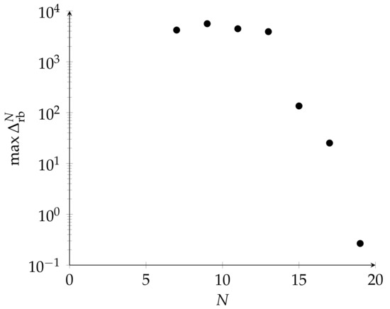
Figure 1. Plot of the value of the a posteriori error estimator $\max {\Delta }_{\mathrm{rb}}^N={\max }_{\mu \in \Xi }{\Delta }_{\mathrm{rb}}^N\left(\mu \right)$ during the offline stage computed by the POD-greedy algorithm. The dimension of resulting reduced basis is $N=19$, ${\epsilon }_{\mathrm{tol}}=1$ (Experiment I).

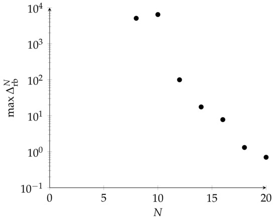
Figure 2. Plot of the value of the a posteriori error estimator $\max {\Delta }_{\mathrm{rb}}^N={\max }_{\mu \in \Xi }{\Delta }_{\mathrm{rb}}^N\left(\mu \right)$ during the offline stage computed by the POD-greedy algorithm. Dimension of resulting reduced basis is $N=20$ for ${\epsilon }_{\mathrm{tol}}=1$ (Experiment II).

In the experiment, we use an algorithm that intertwines a POD step with a greedy step [17]. We also use a simple POD-based construction of the reduced basis via computation and compression of $U_h\left(\mu \right)$ by sequential sampling of $\mu \in \Xi$ as an alternative offline stage. In this method, we skip the while condition and just do a loop over ℓ in Algorithm 3.

We compare the performance of the POD-greedy algorithm and the sequential sampling POD during the online stage. The results of the two approaches for the offline stage are shown in Table 2 and Table 3 for Experiments I and II. We define the CPU time gain factor as the ratio between the CPU time for the truth solution and the CPU time for its reduced basis approximation, averaged over 10 runs. Increasing the dimension of the reduced basis N decreases the CPU time gain factor.

Table 2. CPU time gain factor and approximation error between the truth and the reduced basis solution at $t=T_{\mathrm{end}}$ with a reduced basis of dimension N. The reduced basis is computed with a POD-greedy algorithm (Experiment I).

$\mathit{\mu }$	CPU Time Gain Factor	${\mathit{L}}_2$-Error	A Posteriori Error
POD-greedy algorithm ($N=19$)
0.04	15.99	$4.02\times {10}^{-4}$	$5.45\times {10}^{-1}$
0.07	17.13	$3.91\times {10}^{-4}$	$3.03\times {10}^{-1}$
0.11	16.96	$3.78\times {10}^{-4}$	$1.83\times {10}^{-1}$
POD with sequential sampling ($N=24$)
0.04	8.80	$8.84\times {10}^{-5}$	$1.92\times {10}^{-1}$
0.07	8.87	$8.35\times {10}^{-5}$	$3.81\times {10}^{-1}$
0.11	8.73	$7.73\times {10}^{-5}$	$5.99\times {10}^{-1}$

Table 3. CPU time gain factor and approximation error between the truth and the reduced basis solution at $t=T_{\mathrm{end}}$ for a reduced basis of dimension N (Experiment II).

$\mathit{\mu }$	CPU Time Gain Factor	${\mathit{L}}_2$-Error	A Posteriori Error
POD-greedy algorithm ($N=20$)
0.04	12.3880	$3.03\times {10}^{-4}$	$5.81\times {10}^{-2}$
0.07	12.3402	$2.69\times {10}^{-4}$	$4.81\times {10}^{-2}$
0.11	13.5057	$2.47\times {10}^{-4}$	$3.76\times {10}^{-2}$
POD with sequential sampling ($N=24$)
0.04	7.6595	$2.25\times {10}^{-4}$	$3.13\times {10}^{-2}$
0.07	7.0407	$2.18\times {10}^{-4}$	$2.89\times {10}^{-2}$
0.11	7.6818	$2.09\times {10}^{-4}$	$2.99\times {10}^{-2}$

The $L^2$ error between the truth solution and its reduced basis approximation at $T_{\mathrm{end}}$ is below the a posteriori error estimator. However, in Experiment I, the difference in errors is of the order 10 ${}^2$:10 ${}^3$, meaning that the error estimator derived in Lemma 2 is not very sharp. The sharpness of the a posteriori estimator ${\Delta }_{\mathrm{rb}}^N$ could be improved by reducing the time step $\tau$, but that would offset the benefits of the implicit integration scheme, requiring more time layers where the Newton iteration must be performed.

5. Conclusions

A reduced basis for approximating the solutions to a spatial Lotka-Volterra model (1) based on the implicit Euler scheme for a Galerkin finite element approximation (3) is constructed by two approaches: a POD-greedy algorithm and a POD with sequential sampling, and their performance is compared. Due to the offline/online decomposition and the low dimension of the constructed reduced basis space, the method leads to significant computational savings.

An a posteriori estimator for the approximation error used for the POD-greedy algorithm is derived based on the chosen scheme for the time integration. The development of a posteriori error estimators for the reduced basis approximation is closely linked to the problem at hand, as has been noted elsewhere in the literature [16,17]. However, its performance in the case of this system of nonlinear reaction-diffusion equations reveals a challenge in terms of the trade-off of sharpness of the estimate and the time integration step.

The presented work attempts to bring forward the problem of generalisability and performance of the reduced basis method to nonlinear evolution models motivated by biological or biomedical applications. The development of appropriate methods that produce near-real-time approximation of the solutions to such models at low computational effort could serve contexts such as cancer therapy and increase the applicability of mathematical models to emerging fields such as personalized treatments.

References

- Pascarella, G.; Kokkinakis, I.; Fossati, M. Analysis of transition for a flow in a channel via reduced basis methods. Fluids 2019, 4, 202. [Google Scholar] [CrossRef] [Green Version]
- Nonino, M.; Ballarin, F.; Rozza, G. A monolithic and a partitioned, reduced basis method for fluid-structure interaction problems. Fluids 2021, 6, 229. [Google Scholar] [CrossRef]
- Veroy, K.; Prud’homme, C.; Patera, A.T. Reduced-basis approximation of the viscous Burgers equation: Rigorous a posteriori error bounds. C. R. Acad. Sci. Paris Ser. I 2003, 337, 619–624. [Google Scholar] [CrossRef]
- Veroy, K.; Patera, A.T. Certified real-time solution of the parametrized steady incompressible Navier–Stokes equations: Rigorous reduced-basis a posteriori error bounds. Int. J. Numer. Methods Fluids 2005, 47, 773–788. [Google Scholar] [CrossRef]
- Akkari, N.; Casenave, F.; Moureau, V. Time stable reduced order modeling by an enhanced reduced order basis of the turbulent and incompressible 3D Navier-Stokes equations. Math. Comput. Appl. 2019, 24, 45. [Google Scholar] [CrossRef] [Green Version]
- Grepl, M.A.; Patera, A.T. A posteriori error bounds for reduced-basis approximations of parametrized parabolic partial differential equations. Math. Model. Numer. Anal. 2005, 39, 157–181. [Google Scholar] [CrossRef] [Green Version]
- Haasdonk, B.; Ohlberger, M. Reduced basis method for finite volume approximations of parametrized linear evolution equations. Math. Model. Numer. Anal. 2008, 42, 277–302. [Google Scholar] [CrossRef]
- Haasdonk, B.; Ohlberger, M.; Rozza, G. A reduced basis method for evolution schemes with parameter-dependent explicit operators. Electron. Trans. Numer. Anal. 2008, 32, 145–168. [Google Scholar]
- Andrew, S.M.; Baker, C.T.; Bocharov, G.A. Rival approaches to mathematical modelling in immunology. J. Comput. Appl. Math. 2007, 205, 669–686. [Google Scholar] [CrossRef]
- Bocharov, G.; Volpert, V.; Tasevich, A. Reaction-diffusion equations in immunology. Comput. Math. Math. Phys. 2018, 58, 1967–1976. [Google Scholar] [CrossRef]
- Eladdadi, A.; Kim, P.; Mallet, D. (Eds.) Mathematical Models of Tumor-Immune System Dynamics; Springer: New York, NY, USA, 2014. [Google Scholar] [CrossRef]
- Enderling, H.; Chaplain, M.A. Mathematical modeling of tumor growth and treatment. Curr. Pharm. Des. 2014, 20, 4934–4940. [Google Scholar] [CrossRef] [PubMed] [Green Version]
- Carrère, C. Optimization of an in vitro chemotherapy to avoid resistant tumours. J. Theor. Biol. 2017, 413, 24–33. [Google Scholar] [CrossRef] [PubMed] [Green Version]
- Cantrell, R.; Cosner, C. On the uniqueness and stability of positive solutions in the Lotka-Volterra competition model with diffusion. Houst. J. Math. 1989, 15, 341–361. [Google Scholar]
- Ciarlet, P.G. The Finite Element Method for Elliptic Problems. In Classics in Applied Mathematics; SIAM: Philadelphia, PA, USA, 2002. [Google Scholar]
- Hesthaven, J.S.; Rozza, G.; Stamm, B. Certified Reduced Basis Methods for Parametrized Partial Differential Equations; Springer International Publishing: Cham, Switzerland, 2016. [Google Scholar]
- Quarteroni, A.; Manzoni, A.; Negri, F. Reduced Basis Methods for Partial Differential Equations: An Introduction; Springer International Publishing: Cham, Switzerland, 2016. [Google Scholar]
- Quarteroni, A.; Valli, A. Numerical Approximation of Partial Differential Equations; Springer: Berlin/Heidelberg, Germany, 2008. [Google Scholar]
- Hecht, F. New development in FreeFem++. J. Numer. Math. 2012, 20, 251–265. [Google Scholar] [CrossRef]
Publisher’s Note: MDPI stays neutral with regard to jurisdictional claims in published maps and institutional affiliations. |
© 2022 by the author. Licensee MDPI, Basel, Switzerland. This article is an open access article distributed under the terms and conditions of the Creative Commons Attribution (CC BY) license (https://creativecommons.org/licenses/by/4.0/).